SAIC-98/1010

"GLOBAL MAGNETOHYDRODYNAMIC

MODELING OF THE SOLAR CORONA"

FINAL REPORT

(2/07/95--2/06/98)

m _J_w ....

_ Immm_

Science Applications International Corporation

An Employee-Owned Company

NASA CONTRACT: NASW-4968

SPACE PHYSICS SUPPORTING RESEARCH AND TECHNOLOGY (SR&T),

AND SUBORBITAL PROGRAM

PRINCIPAL INVESTIGATOR"

JON A. LINKER

SCIENCE APPLICATIONS INTERNATIONAL CORPORATION

10260 CAMPUS POINT DRIVE

SAN DIEGO, CA 92121-1578

10260 Campus Point Drive, San Diego, California 92121 (619) 546-6000Other SAIC Offices. Albuquerque, Boston, Colorado Springs, Dayton, Huntsville, Las Vegas, Los Angeles, McLean, Oak Ridge, Orlando, Pale Alto, Seattle, and Tucson

https://ntrs.nasa.gov/search.jsp?R=19980107903 2020-03-11T13:16:28+00:00Z

Global Magnetohydrodynamic Modeling of the Solar Corona

NASA Contract NAS_vV-4968 (2/07/95-2/06/98)

P.I." Jon Linker

Final Report

1. Introduction

The corona.1 magnetic field defines the structure of the solar corona, the position

of the heliospheric current sheet, the regions of fast and slow solar wind, and the

most likely sites of coronal ma.ss ejections. There are few measurements of the

maginetic fields in the corona, but the line-of-sight component of the global magnetic

fields in the photosphere have been routinely measured for many years (for example,

at Stanford's \Vilcox Solar Observatory, and at the National Solar Observatory

at Kitt Peak). Tile SOI/MDI instrument is now providing high-resolution full-

disk magnetoggrams several times a da,y. Understanding i the la.rgge-scale structure of

the solar corona and inner heliosphere requires accurately mapping the measured

photospheric magnetic field into the corona and outward.

Ideally, a model should not only extrapolate the magnetic field, but should

self-consistently reconstruct both the plasma and magnetic fields in the corona, and

solar wind. Support from our NASA SR_T contract has allowed us to develop

three-dimensional maginetohydrodynamic (MHD) computations of the solar corona

that incorporate observed photospheric magnetic fields into the boundary condi-

tions. These calculations not only describe the magnetic field in the corona and

interplanetary space, but also predict the plasma properties as well. Our compu-

rations thus far have been successful in reproducing many aspects of both coronal

and interplanetary data, including; the structure of the streamer belt, the location

of coroual hole boundaries, and the position and shape of the heliospheric current

sheet.

The most widely used technique for extrapolating the photospheric magnetic

field into the corona and heliosphere are potential field models, such as the potential

field source-surface model (PFSS) (Schatten et al., 1969; Alt_chuler and Newkir]_,

1969; IIock._em.a: 1984, 1991) and the potential field current-sheet (PFCS) model

( Schatten, 1971 ).

The potential field models have been shown to describe many aspects of coro-

nal and interplanetary data (e.g., Wang and Sheeley, 1988" Hoek_ema and Sues,s,

1990" Wang and Sheele_], 1992), and the models are still being improved (Schulz,

1995" Zhao and Hoek,_ema, 1995). Ease of computation makes these models es-

pecially useful tools, but the simplifying assumptions underlying these methods

limit their applicablility. Tile coronal phenomena of interest are large-scale and

long-wavelength, and are thus well described by the magnetohydrodynamic (bIHD)

equations. Magnetostatic solutions (Bogdan and Low, 1986; Bagenal and Gibson,

1991; Gib_on and Bagenal, 1995; Gib_on et al., 1996) can describe the density

distribution in the lower corona but cannot model the solar wind. Full MHD com-

putations (including flow terms) contain much of the physics required for describing

the solar corona and inner heliosphere. At the inception of our NASA-supported

project, MHD computations of helmet streamers had been performed for many years

(e.g.. Endler, 1971" Pneuman and Kopp, 1971; Steinolfaon et al., 1982; Washimi et

al., 1987; Linker et al., 1990" Wang et al., 1993; Linker and Mikid, 1995; Stewart

and Bravo, 1996). However, these calculations typically used idealized magnetic

flux distributions (such as a dipole or other multipole component), and most were

limited to two dimensions. The resulting configurations could only be compared to

the corona in terms of abstract qualities, and not specific observations.

To perform a realistic 3-D MHD computation of the corona, it is necessary

to incorporate realistic magnetic fields into the boundary conditions (Mikid and

Linker. 1996: Linker et al., 1996: U_manov, 1996). We have developed numerical

XIHD computations of the corona and inner heliosphere that incorporate observed

photospheric magnetic fields. In Section 2, we briefly describe the methodology of

our computations. Section 3 shows comparisons of our results with specific obser-

vations. Section 4 describes improvements to the model that are presently being

investigated.

2. Modeling the Corona and Inner Heliosphere

To compute self-consistent three-dimensional MHD solutions for the large-scale

corona, we solve the following form of the equations in spherical coordinates (Mikid

and Lin_:er, 1994. describes the method)"

VxB- 47rj (1)c

1 0B=-Vxn (2)

c c0t

vxBE+ =r/J (3)

C

Op

+ V-(pv) --0 (4)

(0v ) !jp -_-+v. Vv - c ×B-Vp-Vpw+pg+V.(upVv) (5)

+ v. (pv)- - i)(-pV,v + s) (6)

where B is the magnetic field intensity, J is the electric current density, E is the

electric field: v, p, and p are the plasma velocity, mass density, and pressure. The

gravitational acceleration is g, 7 is the ratio of specific heats, r/ is the resistivity, u is

the viscosity, S represents energy source terms, and the wave pressure p.w represents

the acceleration due to Alfv_n waves [Jacques, 1977; Hollweg, 1978].

The term S in equation (6) includes the effects of coronal heating, thermal

conduction parallel to B, radiative losses, and AlfvOn wave dissipation (viscous and

resistive dissipation can also be included). S and Pw were set to zero for the results

discussed in this section, which restricts us to examining polytropic solutions (i.e.,

dPp-"l/(l_ - 0). Tt/ese solutions have the advantage that relatively simple models

can nlatch many of the properties of the corona: however, values of 7 close to 1

('? - t.05 for the results shown here) are necessary to produce plasma profiles that

are similar to coronal observations (Parker, 1963). This reflects the importance of

the processes embodied in S that we have neglected here. Section 4 describes the

incorporation of these processes.

The methods we use to solve equations (1-6), including the boundary condi-

tions, have been descril)ed I)reviously (Mitcid and Linl_er, 1994, 1996; Lintcer et al.

1996" Linh:er and Milci_, 1997). We have used synoptic magnetograms from the

\\:ilcox Solar Observatory at Stanford and the National Solar Observatory a.t Kitt

Peak (collected during a solar rotation by daily measurementsof the line-of-sight

magnetic field at central meridian) to specify the radial magnetic field (B_) at the

photosphere (in the manner describedby Wang and Sheeley, 1992). We also spec-

if)" the density and pressure at the lower boundary. For the initial condition, we

compute the potential (current-fl'ee) field consistent with the specified distribution

of Br at the lower boundary, and a wind solution [Parker, 1963] consistent with the

specified p and p. We then solve equations (1-6). The configuration evolves until a

steady state is reached, when the magnetic field lines and plasma state have settled

into equilibrium. A typical run of our code on a relatively coarse (nonuniform) com-

putational mesh (81 x 51 x 32 r,O,O mesh points) takes about an hour of Cray-C90

CPU time per day of real time. while higher-resolution runs (101 x 101 x 64) take

a few hours of CPU time per day of real time. Coronal computations relax to a

steady state in a few days of real time.

3. Comparisons with Observations

The solutions obtained in the manner described in Section 2 can in principle

provide a 3-D description of the corona and inner heliosphere, including the detailed

distribution of magnetic fields, currents, plasma, density, and temperature. The

validity of this approach can only be verified through comparison with observations.

With this goal in mind we have sought to compute solutions for specific time periods

of interest. Carrington rotation 1S92 (CR1892, January 27-February 23, 1995) is

good example: a variety of coronal data is available for that time period (Mauna Loa

white light images. Yohkoh soft X-ray images, and coronal hole boundaries based

on the Kitt Peak 10830 images). At the same time Ulysses probed the heliosphere

over a wide range of latitudes. 'V\_ used a Kitt Peak synoptic map to specify B_ in

the manner described in Section 2, and computed a solution out to 400 solar radii

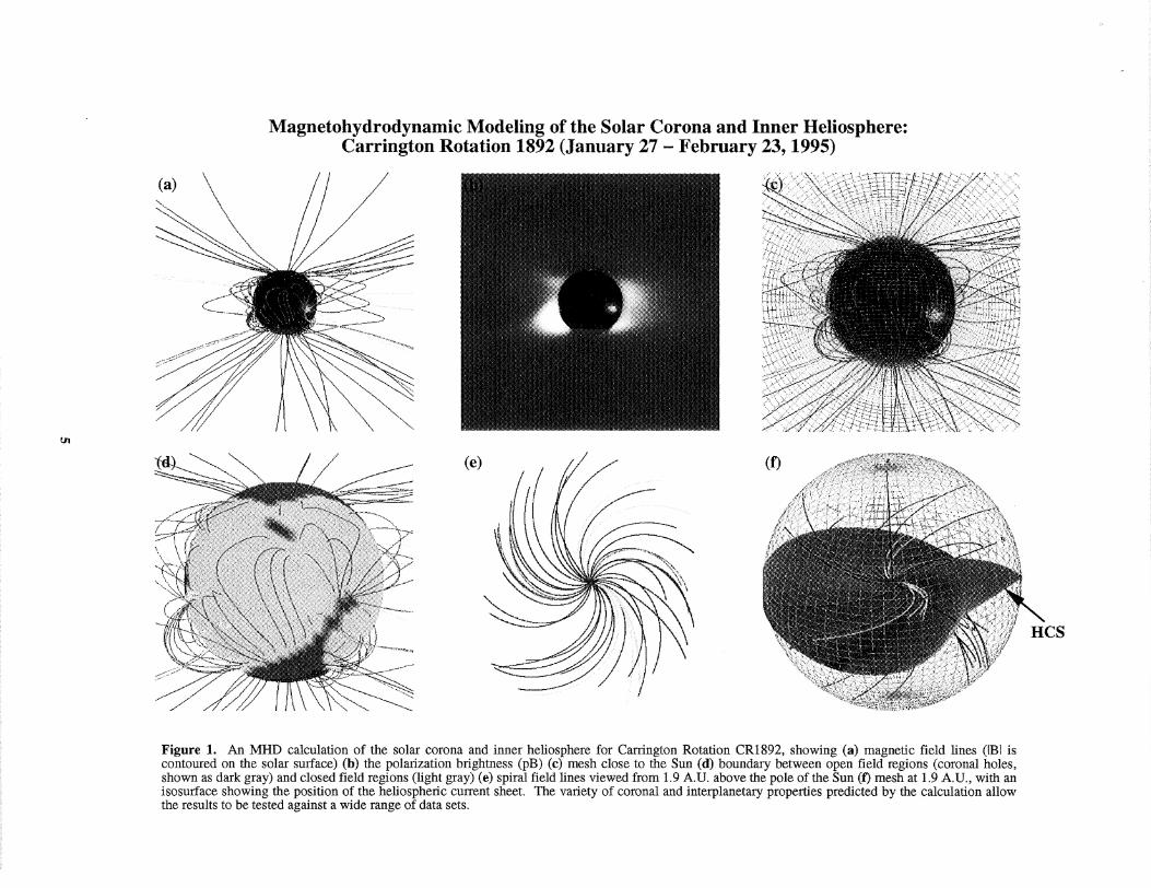
(1.9 astronomical units, or A.U.). Figure 1 shows how the solution captures coronal

structures near the Sun and also models the inner heliospere.

Coronal or hehnet streamers appear as bright regions in white-light coronal im-

ages; they are believed to outline closed magnetic regions on the Sun. To directly

compare our results with observations, we must develop images like those obtained

Magnetohydrodynamic Modeling of the Solar Corona and Inner Heliosphere:Carrington Rotation 1892 (January 27 - February 23, 1995)

i

Figure 1. An MHD calculation of the solar corona and inner heliosphere for Carrington Rotation CR1892, showing (a) magnetic field lines (IBI iscontoured on the solar surface) (b) the polarization brightness (pB) (c) mesh close to the Sun (d) boundary between open field regions (coronal holes,shown as dark gray) and closed field regions (light gray) (e) spiral field lines viewed from 1.9 A.U. above the pole of the Sun (f) mesh at 1.9 A.U., with anisosurface showing the position of the heliospheric current sheet. The variety of coronal and interplanetary properties predicted by the calculation allowthe results to be tested against a wide range of data sets.

with coronagraphs and during eclipses. Frequently the polarization brightness (pB)

is the observed quantity. The distribution of pB in the plane of the sky is pro-

portional to the line-of-sight integral of the product of the electron density and a.

scatt cring function that varies along the line of sight (Billir_9_ , 1966). Using the

plasnla density fl'om our coml_utation, we can calculate pB and compare it with

actual observations. Eclipse and coronagraph images typically compensate for the

rapid fall off of coronal density, through the use of radially graded filters or the

vignetting properties of the coronagraph. We detrend our computed pB in a similar

manner. Figure 2 shows a comparison between the predicted pB from our computa-

tion with Mauna Loa Coronameter data. Throughout the rotation, the results from

tile MHD computation correspond well with the observations. This computation,

along with those we have performed for other time periods, support the long-held

belief that the magnetic field distribution on the Sun controls the position and shape

of the streamer belt.

Open field regions on the Sun (coronal holes) are the source of the solar wind.

Another way we can test the MHD model is to compare open field regions from

the computation with coronal holes observed from solar images. By tracing field

lines at each grid point and determining whether the field lines were open (reached

the outer boundary) or closed (returned to the Sun), we mapped the open field

regiolls predicted by our computation and compared them with Yohkoh soft X-ray

images, as shown in Figure 3. Coronal holes typically show" up as dark regions

in X-rays. Throughout the rotation, the coronal hole boundaries predicted by the

model agree reasonably well with the dark regions seen in Yohkoh, although there

are also some discrepancies. It is important to note that the identification of coronal

holes in soft X-ray images (or the I(itt Peak 10830 line) is somewhat subjective.

In X-rays, neighboring coronal emission can obscure coronal holes, and the absence

of emission can also occur in quiet closed field regions. As part of a. coordinated

stll(12, for the time period of the Ulysses fast latitude scan (Neugeba'_ter et al., 1997),

the coronal hole bolmdaries from our model were also compared with the He 10830

ol)servations fi'om I(itt Peak. Reasonable correspondence was again found, although

it is interesting to note that not only were there some disagreements between the

Comparison of a 3D MHD Model of CR1892 with Mauna Loa Coronameter Data (HAO)

January 28,1995 February 4, 1995 February 10, 1995 February 14, 1995 February 21, 1995

!

iObservations of Polarization Brightness (Mauna Loa MK3)

• __

Polarization Brightness (Mill) Model)

"_-b'<_...."\ //'/ _"" ....... " ...._\1,.\_ /_z"".... . .... _.._.\_\ \\_ 4>:..'._-i""..-_;_i_ _

....... _.................._........... .....==,_

j<,>.-_._- _]--_ .-

/ ,;;'/" I! \ , \\ \

Field Lines (MHD Model)

Figure 2. Comparison of Mauna Loa Coronameter data (top panels) with the polarization brightness (pb) computed from the MHDsimulation (middle panels). The model results correspond well to the observations throughout the rotation. In the bottom set of panelstraces of the magnetic field lines are shown, with the magnitude of the magnetic field contoured on the solar surface. The strongestfields (yellow colors) correspond to active regions.

Comparison of Coronal Hole Boundaries: A 3D MHD Model of CR1892 and Yohkoh Data

January 28,1995 February 4, 1995 February 11, 1995 February 15, 1995

l

...._i:_5"i?iiiii@iii@iiii7

,_-_",:_!i_;;_i!!!!!!!!!ii_{i!i,,.__ ___"!,V_i.==-

mYohkoh Soft X-Ray Data

/ _'"-... \.\ / _..-_---

!i_!7]>,:7(',.;.:.?',_777_if_::';t_._"]

i_jii!_!_i_:_. ',..

\/

7ii!iIi!ii!?!;i!iill

Field Lines and Coronal Hole Boundaries (MHD Model)

February 22, 1995

....i ;:,::..__-t/ _'-.. _ _' 1

• '1_71;#;;717)77111ii111!7..,"_"

Figure 3. Comparison of Yohkoh soft X-ray images (top panels) with the open field regions predicted by the MHD simulation.Identification of coronal hole boundaries in Yohkoh data can be somewhat subjective. The darkest regions often correspond to coronalholes (although the absence of emission can occur in closed field regions, and coronal holes can be obscured by neighboring emission).Nevertheless, the coronal hole boundaries predicted by the MHD calculation (shown in dark gray) correspond approximately to thoseseen in the Yohkoh data.

coronal holes predicted by the model and the absence of emission in the observations,

coronal hole boundaries in He 10830 and the dark regions in Yohkoh also did not

always correspond.

The comparisons of our results with coronal data. shows that the basic large-scale

structure of the corona has been captured in the model. We have also compared

our results with interplanetary data. During February-April, 199,5 (Carrington ro-

tations 1892-1894), the Ulysses spacecraft sampled a wide range of heliographic

latitude in a relatively short period of time; this time period has since been referred

to as the fast latitude scan. Figure 4 (red curve) shows "simulated" Ulysses data,

created by flying the Ulysses trajectory through the MHD solution and extracting

/),. along the trajectory. For comparison, the actual B_ measured by Ulysses is also

shown (blue curve). The fluctuations in the solar wind data are caused by turbulent

waves and transient phenomena, and thus are not present in the MHD model, but

the model does reproduce the correct magnitude and polarity of the field, includ-

ing many of the heliospheric current sheet crossings. Not surprisingly, the model

matches the data best during and shortly after CR1892, when the photospheric

data used to perform the calculation is most applicable. Photospheric data for the

subsequent rotations shows that the magnetic field is indeed evolving.

Figure 5 shows the heliospheric current sheet predicted by our computation for

CR1892. depicted as an isosurface. The Ulysses trajectory in the rotating frame of

the Sun is shown. Blue colors for the trajectory correspond to times when negative

Br fields were observed, and red colors show times when positive B_ fields were

ol)served. The dominant polarity observed by Ulysses agrees with that predicted

1)3,,the simulation for most of the early (lower) part of the trajectory. In the later

part of the trajectory, there is a passage into negative polarity not predicted by the

model (this can also be seen in Figure 4 around day-of-year 85). As this occurred in

CFt1894, it is possible that the heliospheric magnetic field has changed significantly

from C1R1892 (two months earlier). To test this possibility, we computed XIHD

models for rotations CR1893 and CR1894 as well. Figure 6 shoves a comparison

of heliospheric current sheet (HCS) crossings observed by Ulysses and projected

l_ack to the Sun (Smith et al. 1995) with the HCS predicted by the MHD model for

Magnetic Field Comparison

_ 80 100 1200 20 40 Day-o Year

Figure 4. A comparison of a simulated time series of B r for the MHD computation of CR1892 (red curve) with Ulysses data

(blue curve). Heliospheric current sheet crossings identified by Smith et al. (1995) are marked as crosses (transient phenomena

can also cause B r to change sign). The time period for CR1892 (when the photosphenc data used by the MHD calculation is

most applicable) is marked on the plot. The MHD calculation reproduces the correct magnitude of the field and matches manyof the cun'ent sheet crossings. Not surprisingly, the MHD results match the data best during or close to the CR1892 time

period.

Ulysses Trajectory Shown with a HeliosphericCurrent Sheet Computed Using a 3D MHD Model

Red: B r > 0 Ulysses Trajectory

Blue: Br < 0

k__

Heliospheric Current SheetFast Latitude Scan (Jan. - Apr. 1995)Carrington Rotations 1892, 1893, 1894

Figure 5. The heliospheric current sheet (HCS) predicted by the MHD computation of CR1892 shown in Hgure 1. The

Ulysses trajectory (red and blue curve) is shown in the rotating frame of the Sun. The colors of the trajectory indicate thepolarity of the magnetic field obse_ared by Ulysses. Fluctuations in B r are present because of waves and transients in the solar

wind, but the dominant polarity observed by Ulysses is similar to that predicted by the MHD computation.

Comparison of MIlD Computations of CR1892, CR1893, and CR1894with Ulysses Heliospheric Current Sheet (HCS) Crossings

•_ 40 _''''' ' '''' '' '''''''' '' ' ''

20

"_ ---"._-. -._.___ o

_ -20

-40

|

0 45 90 135 1 B0 225 270 :315 360

Longitude

Figure 6. The HCS predicted by MHD computations of CR1892, CR1893, and CR1894 (red, blue, and green curves) and theUlysses trajectory during this time (red, blue, and green fines) projected back at the Sun. HCS crossings from Ulyssesidentified by Smith et aL (1995) (also projected back to the Sun) are shown as crosses. There is overall good agreement

between the predicted HCS crossings (where the Ulysses trajectory intersects the computed HCS) and the observed crossings.The MHD calculations predict that the HCS moved higher in latitude in the north during CR1894, as seen in the data.

However, the uppermost crossings observed by Ulysses are not predicted by the model. Sensitivity of the calculations to the

polar fields (poorly determined by fine-of-sight magnetograms) could be a possible reason for this difference.

9

the two rotations. The red, blue and green straight lines show the Ulysses trajec-

tory for CR1892, CR1893, and CR1894, respectively, and the red, blue, and green

curves show the predicted HCS for these rotations. There is overall good agreement

between the predicted H CS crossings (where the Ulysses trajectory intersects the

model HCS) and the observed crossings (marked as +). The MHD calculations

based on the photospheric data for CRt893 and CR1894 predict that the helio-

spheric magnetic field should have evolved during this time period and that the

HCS should have moved to higher northern latitudes for CR1894, consistent with

the observations. However, the two uppermost crossings are still not predicted by

the model. We note that the tilt of the HCS (and thus its extent in northern and

southern latitudes) can be strongly influenced by the polar fields, which are not well

determined by line-of-sight magnetograms.

We have also computed MHD solutions for a number of other time periods

of interest, including the last three total solar eclipses (see Figure 7). These and

other comparisons of our MHD solutions with observations show that the MHD

model typically does a. good job of reproducing many aspects of coronal structure.

While the success of the model has been encouraging, there is still significant room

for improvement. In the next section, we describe how we are working refine and

extend the physics in our computations to provide a tool capable of addressing

important aspects of coronal structure that are beyond the scope of the present

model.

4. An Improved Model of the Corona and Solar Wind

Starting at the photosphere and rising upward into the solar atmosphere, the

temperature rises steeply in the chromosphere and transition region. The detailed

coronal heating mechanism is not yet understood (see Parker, 1994 for a recent

review), but most coronal heating mechanisms imply that this sharp temperature

rise is the result of a volllmet.ric heat source in the corona. In the inner corona, the

large parallel thermal conductivity tends to make the temperature relatively uniform

(on the order of 1-2x106 °K). The density at the top of the transition region is

determined by the balance between radiation loss in the chromosphere and heating

10

Field Lines (MHD Model)

ECLIPSE COMPARISONS

Polarization Brightness (MHD Model) Observations

November 3, 1994 Eclipse Image, HAO Expedition to Chile

October 24, 1995 Eclipse Image, F. Diego and S. Koutchmy

March 9, 1997 LASCO C2 Coronagraph Image

Figure 7. Comparison of MHD computations of the solar corona with eclipse observations. For the November 3, 1994 solar eclipse, we used asynoptic magnetoglam for Carrington rotation 1888 (October 10 - November 6, 1994) as boundary conditions for the model, and we comparedwith the results subsequent to the eclipse. For the October 24, 1995 and March 9, 1997 solar eclipses, we used synoptic magnetograms from therotation prior to the eclipse (CR1900: September 2 - September 29, 1995, and a combination of CR1918 and 1919: January 30 - February 26,1997) to predict the structure in advance. All of these calculations used synoptic magnetograms from the Wilcox Solar Obsevatory. For the March9 eclipse, no eclipse data is yet available. Comparison with an image from the LASCO coronagraph aboard the SOHO spacecraft is shown. Theseand other coronal modeling results can be found on our WEB page: http://iris023.saic.com:8000/corona/modeling.hmal

1)y thermal conduction fl'om the hot corona ( Withbroe, 1988). As we extend into the

outer solar corona and interplanetary medium, the temperature decreases slowly as

a result of solar wind acceleration and thermal conduction losses. Beyond about

10 R._ (where R_ is the solar radius), the plasma becomes collisionless, reducing

tlle thermal conduction (Hollweg, 1978). In this region, solar wind acceleration by

Atfvdn waves can be important, and may be necessary to produce the observed fast

solar wind at. 1 A.U.

For the solutions described in Section 2, the use of a polytropic energy equation

with a reduced polytropic index 3' is an attempt to combine all these effects into

a simplified energy equation. However, not surprisingly, this simple model fails to

reproduce the fast (_ S00 km/s) and slow (_ 400 km/s) wind streams that are

measured in interplanetary space. The nearly uniform coronal temperature that

results from this model implies that the density scale height does not change much

between the open and closed field regions, and so the magnitude of the density

contrast between coronal holes and streamers is also not reproduced.

It is the complicated interplay of radiation loss, thermal conduction, coronal

heating, and Alfv(_n wave acceleration and dissipation that describes the accelera-

tion of the solar wind from the inner solar corona, into the heliosphere. Fortunately,

we can benefit from the considerable amount of research that has already been per-

formed with one-dimensional MHD and multi-fluid models ( Withbroe, 1988; Habbat

et al.. 1995). These models have been quite successful, despite their obvious geo-

metrical limitations, in modeling thermodynamic processes in the solar wind and

in comparisons with spacecraft solar wind measurements (E._ser and Habbal, 1995"

Habbal et al., 1996). The prescription for improving our coronal model follows nat-

urally from existing 1-D models, and requires the inclusion of the effects described

above in the energy and momentum equations of the 3-D MHD model. Some of

these effects (heating and thermal conduction) have previously been included in

2-D MHD models (Su.e._s e.t a,1.. 1996). The advant.age of a multi-dimensional MHD

calcula.tion is that the magnetic field geometry (i.e., the location and distribution

(-)f open and closed field regions) is determined self-consistently, eliminating the

parameters in the 1-D models that specify the flux tube geometry (the so-called

12

"expansion factor"). As has been done in 1-D models, the inner boundary is now

chosen to be within the transition region, at a temperature of To -500,000°K.

The balance of radiation loss and thermal conduction within the chromosphere and

transition region determines the density at the inner boundary from the condition

( Withbroe, 1988)

JT{ ° 1Cn_T o QtT)T 1/' dT - -q2o(Zo ) (7)h 2

where 1,e is the electron density at the inner boundary, C is a known constant,

q0(T0) is the thermal conduction heat flux at To, and the integral is performed from

the base of the chromosphere (at Tch _ 6000°K)through the top of the transition

region (at T- To). The boundary conditions on the velocity are determined from

the characteristic equations (Linker and Milcid, 1995, 1997" Miki_ and Linlcer, 1996).

Therefore, in this formulation, the only boundary conditions required from obser-

vations at the lower boundary r- Rs are on the radial magnetic field.

The energy equation (6) becomes

Op+ V. (pv) - (-/- 1)(-pV. v- V-q- n_npQ(T)+ Hch + D) (8)

0t

,,,'here q - -glll_l_. VT is the parallel (along B) thermal conduction heat flux,

Hch is the coronal heating source, D is the Alfv6n wave dissipation term, ne and

_p are the electron and proton density, and Q(T) is the radiation loss function

(Rosner et al., 1978). The parallel thermal conductivity _i] is the Spitzer value

in the collisional regime, h,iI - 9 x 107T 5/2 [erg/cm2/s], with T in degrees I(, and

is reduced in the collisionless regime (beyond _ 10Rs)" the representation in this

regime is parameterized as a collisionless heat flux (Hollwe9, 1978).

Results from previous 1-D computations suggest that an additional source of

energy and momentum is necessary to accelerate the solar wind. Alfv6n waves of

solar origin are considered to be the most likely candidate (IIollweg, 1978; Withbroe,

1988). The acceleration of the solar wind by Alfv_n waves occurs on a spatial and

time scale that is below the spatial and time resolution of a global numerical model.

In 1-D models, this effect is included using an equation for the time-space averaged

Alfv_n wave energy density e (Jacq_tes, 1977)

0e+V.F = v. Vpu,- D (9)

0t

13

3where F - (_v + VA)e is the Alfv_n wave energy flux, VA -- B/x/4rrp is the Alfv6n

A

speed, v A - -t-bvA is the A1D6n velocity , and pu, - ½e is the Alfvfin wave pres-

sure that appears in the moment.unl equation (g) and represents the force on the

plasma by, Alfv6n waves. To incorporate equation (9) in a multi-dimensional imple-

mentation, it is necessary to transport two Alfv_n wave fields (waves parallel and

antiparallel to B), which are combined to give the Alfv_n wave energy density e. e is

related to the space-time average of the fluctuating component of the magnetic field

(SB by e - (_SB 2)/4ft. The dissipation term D expresses the nonlinear dissipation

of Alfv6n waves in interplanetary space and will be modeled phenomenologieally

(Hollweg, 1978). The term v-Vp_, in eq. (9) is the work done on the Alfv_n waves

by the plasma flow.

The increased complexity of the improved model makes a step-by-step approach

essential. We first incorporated our improved model in a. 1-D code, and reproduced

the results of Withbroe (1988). We have since implemented the model in two di-

mensions, and performed a preliminary comparison between a polytropic model,

a t,hermodynamic model (heating, parallel thermal conduction, and presence of a

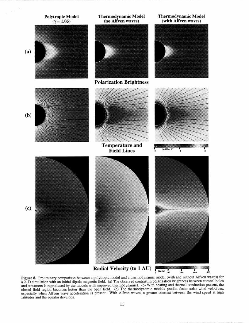
transition region), and a. thermodynamic model with Alfv_n waves. Figure 8 shows

this comparison. With the improved thermodynamic model, the observed white

light contrast between coronal holes and streamers is reproduced (Bagenal et al.

1996). and the wind achieves faster velocities. With Alfv4n waves, a larger contrast

between the fast and slow wind develops.

The improved model significantly advances our capabilities to study the large-

scale corona and inner heliosphere. The trade-off is that some of the important

physical processes are poorly understood (coronal heating, Alfv4n wave dissipation,

and collisionless thermal conduction) and must be parameterized. In the results

shown in Figure S. the coronal heating was parameterized as

Hch -- Ho(O) p [-(; - (10)

where H0(O) expresses the latitudinal variation of the volumetric heating, and A(0)

expresses the latitudinal variation of the heating flmction scale length. For the cases

shown in Figure 8, H0, ,_, and the flux of Alfv_n waves were assumed to be uniform

14

Polytropic Model(_,- 1.o5)

Thermodynamic Model(no Alfven waves)

Thermodynamic Model(with Alfven waves)

(a)

Polarization Brightness

:! ...............z_!iiiiiiilliiiiii!iii!iiiiiiiiiiii!_i_i

(b)

iii!iiiii!ii!iiiiiiiiiiiiiiiiiiii!i!iiiiiiii!iiiiiiii!iiiii!i!iiiiii_!

i_iiiii_ili!ii!ii_ii!_ii!iiiiiiiiii:

fill:ill........................

(c)

Radial Velocity (to 1 AU) __i_0

Figure 8. Preliminary comparison between a polytropic model and a thermodynamic model (with and without Alfven waves) for

a 2-D simulation with an initial dipole magnetic field. (a) The observed contrast in polarization brightness between coronal holesand streamers is reproduced by the models with improved thermodynamics. (b) With heating and thermal conduction present, the

closed field region becomes hotter than the open field. (c) The thermodynamic models predict faster solar wind velocities,especially when Alfven wave acceleration is present. With Alfven waves, a greater contrast between the wind speed at high

latitudes and the equator develops.

15

in latitude. In the future, weplan to study the effectsof the different parameters in

2-D, and change the coronal heating to be expressed in terms of magnetic topology

(i.e.. a proxy for open and closed field regions) rather than latitude 0. Eventually

we plan to incorporate the improved thermodynamics into full 3-D solutions, just

as we have previously done with the polytropic model.

5. Publications

Crooker, N. U., A. H. McAllister, R. J. Fitzenreiter, J. A. Linker, D. E. Larson,

K. W. Ogilvie, R. P. Lepping, A. Szabo, J. T. Steinberg, A. J. Lazarus, Z. Mikid,

and R. P. Lin, Sector boundary transformation by an open magnetic cloud, sub-

mitted to J. Geophy_. Rea., 1998.

Linker, J. A., &: Mikid, Z., Disruption of a helmet streamer by photospheric shear,

Astrophya. J, 438, L45, 1995.

Linker. J. A., Z. Mikid & D. D. Schnack, Global coronal modeling and space weather

prediction, in Solar Drivers of Interplanetary and Terrestrial Diaturbancea, (K. S.

Balasubramaniam, S. L. Keil, & R. N. Smartt, eds.), Astron. Soc. Pac. Conf.,

95, 208, 1996.

Linker, J. A., and Z. Mikid, Extending coronal models to Earth orbit, in Coronal

Ma._s Ejection_, edited by N. Crooker, J. A. Joselyn, and J. Feynman, Geophya.

Monogr. Set., 99, 269, 1997.

Linker. J. A.. Z. Mikid, D. A. Biesecker, R. J. Forsyth, S. E. Gibson, A. a. Lazarus,

A. Lecinski, P. Riley, A. Szabo, and B. J. Thompson, Magnetohydrodynamic

modeling of the solar corona during Whole Sun Month, in preparation, 1998.

Mikid. Z., & J. A. Linker, Large scale structure of the solar corona and inner

heliosphere, Solar Wind 8, AIP Conf. Proceedings 382, 104, 1996.

),Iikid, Z., &: J. A. Linker, The initiation of coronal mass ejections by magnetic

shear, in Coronal Ma_a Ejections: Cause_ and Consequences, in press, 1997.

Neuo_;el)auer, M., R. J. Forsyth, A. B. Galvin, K. L. Harvey, J. T. Hoeksema, A. J.

Lazurus, R. P. Lepping, J. A. Linker, Z.Mikid, R. yon Steiger, Y. *I. Wang,

and R. F. Wimmer-Schweingruber, The spatial structure of the solar wind and

comparisons with solar data and models, J. Geophys. Re_,., in press, 1998.

16

Van Hoven, G., J. A. Linker, and Z. Mikid, The evolution, structure, and dynamics

of the magnetized solar corona, Gather-Scatter, 11, 6, 1995.

This contract partially or fully supported 9 invited and 15 contributed presentations

at scientific meetings from February, 1995 to February, 1998. Some of our results can

t)e viewed on our \VEB page: httl)'//irisO23.saic.com:SOOO/corona/modeling.html

17

6. References

Altschuler,

Bagenal, F.

Bagenal, F.

Billings, D.

M.D., & G. Newkirk, Sol. Phys., 9, 131 (1969).

, J. A. Linker, & Z. Miki6, EOS Trans AGU, (abstract), 77, $218 (1996)., & S. Gibson, J. Geophys. Res., 96, 17663-17674 (1991).

E., Guide to the Solar Corona, Academic Press, p. 232, 1966.

Bogdan, T. J., & B. C. Low, Astrophys. J., 306,271 (1986).Endlcr, F., Ph. D. _esis, Gottingen Univ. (1971).

Esser, R., & S. R. Habbal, Geophys. Res. Lett., 22, 22661 (1995).

Feynman, J., & S. F. Martin, J. Geophys. Res., 100, 3355 (1995).

Gibson, S., & F. Bagenal, J. Geophys. Res., 100, 19865-19880 (1995).

Gibson, S., F. Bagenal, & B. C. Low, J. Geophys. Res., 101, 4813-4823 (1996).

Habbal, S. R., R. Esser, M. Guhathakurta, & R. Fisher, Geophys. Res. Left., 22, 1465 (1995).

Habbal, S. R., R. Esser, M. Guhathakurta, & R. Fisher, in Solar Wind 8, (D. Winterhalter, J. T. Golsing,S. R. Habbal, W. S. Kurth, & M. Neugebauer eds.) AlP Conf. Proceedings, 382, 129, (1996).

Hoeksema, J. T., Tech. Rep. CSSA-ASTRO-84-07, Center for Space Science and Astronomy, Stanford University,California (1984).

Hoeksema, J. T., Tech. Rep. CSSA-ASTRO-91-01, Center for Space Science and Astronomy, Stanford University,California (199 I).

Hoekscma, J. T., & S. T. Suess, Mem. S.A.It., 61,485 (1990).

Hollweg, J. V., Rev. Geophys. Space Phys., 16, 689 (1978).Jacques, S. A., Ap. J., 215, 942 (1977).

Linker, j. A., G. Van Hoven, & D. D. Schnack, Geophys. Res. Lett., 17, 2281 (1990).Linker, J. A., & Z. Miki6, EOS Trans. AGU, 75, 281 (1994).

Linker, J. A., & Z. Miki6, Astrophys. J., 438, L-45 (1995).

Linker, J. A., Z. Miki6, & D. D. Schnack, in Solar Drivers of Interplanetary and Terrestrial Disturbances, (K. S.Balasubramaniam, S. L. Keil, & R. N. Smartt, eds.), Astron. Soc. Pac. Conf., 95, 208 (1996).

Linker, J. A., & Z. Miki6, in _oronal Mass Ejections: Ca_ttses and Conse__uences, in press, 1997.Miki6, Z., & J. A. Linker, Astrophys. J., 430, 898 (1994).

Miki6, Z., J. A. Linker, & D. D. Schnack, in Solar Drivers of Interplanetary and Terrestrial Disturbances, Astron.Soc. Pac. Conf., 95, 108 (1996).

Miki6, Z., & J. A. Linker, Solar Wind 8, AlP Conf. ProceeAings 382, 104, 1996.

Miki6, Z., & A. N. McClymont, in Solar Active Region Evolution: Comparing Models with Observations (K. S.Balasubramaniam & G. W Simon, eds), Astron. Soc. Pac. Conf. 68, 225 (1994).

Neugebauer, M., R J. Forsyth, A. B. Galvin, K. L. Harvey, A. J. Lazurus, R. P. Lepping, J. A. Linker, Z. Miki6,R. von steiger, Y. M. Wang, & R. F. Wimmer, EOS Trans. AGU, (abstract), 78, $258, 1997.

Parker, E. N., Interplanetary Dynamical Processes, Interscience publishers, New York (1963).

Parker, E. N., Spontaneous Current Sheets in Magnetic Fields (New York: Oxford) (1994).Pneuman, G. W., & R. A. Kopp, Solar Phys., 18, 258 (1971).

Rosner, R., W. H. Tucker, & G. S. Vaiana, Ap. J., 220, 643 (1978).

Schatten, K. H., J. M. Wilcox, & N. Ness, Solar Phys., 6,442 (1969).Schatten, K. H., Cosmic Electrodyn., 2, 232 (1971).

Schulz, M., Space Science Rev., 72, 149 (1995).

Smith, E. J., A. Balogh, M. E. Burton, G. Erdos, & R. J. ForsyLh, Geophys. Res. Lett., 22, 3325 (1995).Steinolfson, R. S., S. T. Suess, & S. T. Wu, Astrophys. J., 255, 730 (1982).

Stewart, G. A., & S. Bravo, in Solar Wind 8, (D. Winterhalter, J. T. Gosling, S. R. Habbal, W. S. Kurth, &M. Ncugebauer eds.) AIP Conf. Proceedings_382, 145 (1996).

Suess, S. T., A. H. Wang, & S. T. Wu, J. Geophys. Res., 101, 19957 (1996).

Usmanov, A. V., in Solar Wind 8, (D. Winterhaltcr, J. T. Gosling, S. R. Habbal, W. S. Kurth, & M. Neugebauereds.), AlP Conf. Proceedings, 382, 141 (1996).

Wang, A. H., S. T. Wu, S. T. Suess, & G. Poletto, Sol. Phys., 147, 55 (1993).

Wang, Y. M., & N. R. Sheeley, J. Geophys. Res., 93, 11,227 (1988).

Wang, Y. M., & N. R. Sheeley, Jr., Astrophys. J., 392, 310 (1992).

Washimi, H., Y. Yoshino, & T. Ogino, Geophys. Res. Lett., 14, 487 (1987).Withbroe, G. L., Astrophys. J., 325, 442 (1988).

Zhao, X., & J. T. Hoeksema, J. Geophys. Res., 100, 19 (1995).

18