The University of Manchester Research

Global glacier dynamics during 100 ka Pleistocene glacialcycles.DOI:10.1017/qua.2018.37

Document VersionAccepted author manuscript

Link to publication record in Manchester Research Explorer

Citation for published version (APA):Hughes, P., & Gibbard, P. L. (2018). Global glacier dynamics during 100 ka Pleistocene glacial cycles. QuaternaryResearch, 90(1). https://doi.org/10.1017/qua.2018.37

Published in:Quaternary Research

Citing this paperPlease note that where the full-text provided on Manchester Research Explorer is the Author Accepted Manuscriptor Proof version this may differ from the final Published version. If citing, it is advised that you check and use thepublisher's definitive version.

General rightsCopyright and moral rights for the publications made accessible in the Research Explorer are retained by theauthors and/or other copyright owners and it is a condition of accessing publications that users recognise andabide by the legal requirements associated with these rights.

Takedown policyIf you believe that this document breaches copyright please refer to the University of Manchester’s TakedownProcedures [http://man.ac.uk/04Y6Bo] or contact uml.scholarlycommunications@manchester.ac.uk providingrelevant details, so we can investigate your claim.

Download date:23. Apr. 2020

1

Hughes, P.D., Gibbard, P.L., 2018. Global glacier dynamics during 100 ka Pleistocene glacial

cycles. Quaternary Research. doi:10.1017/qua.2018.37

Global glacier dynamics during 100 ka Pleistocene glacial cycles

Philip D. Hughes 1, Philip L. Gibbard

2

1 Department of Geography, School of Environment, Education and Development, The

University of Manchester, Oxford Road, Manchester M13 9PL, United Kingdom 2 Scott Polar Research Institute, University of Cambridge, Lensfield Road, Cambridge CB2

1ER, United Kingdom

Abstract: Ice volume during the last ten 100 ka glacial cycles was driven by solar

radiation flux in the northern hemisphere. Early minima in solar radiation combined

with critical levels of atmospheric CO2 drove initial glacier expansion. Glacial cycles

between MIS 24-13, whilst at 100 ka periodicity, were irregular in amplitude and the

shift to the largest amplitude 100 ka glacial cycles occurs after MIS 16. Mountain

glaciers in the mid-latitudes and Asia reached their maximum extents early in glacial

cycles then retreated as global climate became increasingly arid. In contrast, larger ice

masses close to maritime moisture sources continued to build-up and dominated global

glacial maxima reflected in marine isotope and sea-level records. The effect of this

pattern of glaciation on the state of the global atmosphere is evident in dust records

from Antarctic ice cores where pronounced double peaks in dust flux occur in all of the

last eight glacial cycles. Glacier growth is strongly modulated by variations in solar

radiation, especially in glacial inceptions. This external control accounts for ~50-60% of

ice volume change through glacial cycles. Internal global glacier-climate dynamics

account for the rest of the change which is controlled by the geographical distributions

of glaciers.

1. Introduction

The Quaternary is often subdivided on the basis of fluctuations in climate changes, most

recently using the marine oxygen isotope record (Fig. 1), and has been for decades starting in

the 1950s (Arrhenius 1952) with numerous developments since (cf. review in Railsback et al.

2015). This is a record of global ice volume and provides the main basis for defining glacial

cycles (Lisiecki and Raymo 2005). However, it is important to appreciate that this approach

is essentially climatostratigraphy and not chronostratigraphy (Gibbard and West 2000;

Gibbard 2013), although it has been subdivided and defined in chronostratigraphical terms

(e.g. Martinson et al. 1987). The marine isotope record is clearly a valuable global reference

with which the Quaternary can be subdivided and the scheme of stages and substages in

marine isotope record continues to underpin the Quaternary timescale (Lisiecki and Raymo

2005; Railsback et al. 2015) (Fig. 1). Whilst this paper focuses on the Quaternary glacial

cycles, the general principles are also applicable to earlier glacial cycles, such as the mid-

Oligocene Glacial Maximum, and the late Pliocene M2 glaciation (3.3 Ma), both of which are

also defined with reference to the marine isotope record (Harzhauser et al. 2016; De Schepper

et al. 2014).

2

In contrast to the quasi-continuous sedimentary sequences on the deep-ocean floors, the

glacier records on land are inherently fragmentary. At the surface, morphostratigraphical

preservation of glaciations is directly related to the diminishing size of successive glaciations.

In other words if the most recent glaciation is the largest in extent, then evidence for earlier

glaciations will be removed, or at least remoulded or reworked. However, this is not always

the case and it is possible for previous glaciations to be preserved beneath deposits of later

glacier advances or in landscape depressions, especially in lowland environments.

Nevertheless, even in these situations the glacial record is prone to fragmentation. Despite

these challenges, there is direct evidence for glaciations throughout the Quaternary and

before (Ehlers and Gibbard 2007; 2008), although clearly the best potential for dating and

understanding the spatial and climate significance of past glaciers originates from the more

recent Late and Middle Pleistocene glaciations. Ehlers et al. (2011a) found that the

succession of glaciations reported from four of the last ten glacial cycles (Marine Isotope

Stage - MIS 16, 12, 6 and 5d–2) is striking in that it is repeatedly found in numerous areas of

the world, and the absence of records of glaciations during other glacial cycles reflect the fact

that these glaciations were less extensive. Even for the Late Pleistocene the glacier records

are fragmentary and hindered by the fact that successively diminishing glacier extents are

recorded at the land surface. This has been compounded, until recently, by the difficulty in

numerically dating glacial sequences. Recent advances in geochronology, especially

cosmogenic exposure dating and new luminescence techniques, have now revealed a complex

spatial and temporal pattern of glaciation with many areas seeing maximum glacier advances

early in the last glacial cycle, whereas others seeing maximum advances at or close to the

global Last Glacial Maximum (LGM, Hughes et al. 2013).

It is now clear from the last glacial cycle that glacier advances were driven by a complex

interplay of air temperatures and precipitation patterns. Glacier advances are controlled by

the balance between accumulation and ablation, which is largely, though not entirely, driven

by precipitation in the form of snow and summer air temperatures, respectively (Ohmura et al.

1992; Hughes and Braithwaite 2008). This means that glaciers advance depending on the

combination of both accumulation and ablation. For example, many glaciers in the mid-

latitudes and in the continental interiors did not advance through MIS 2 (= Late

Weichselian/Wisconsinan, etc.) and the global LGM but instead suffered retreat. This was

because increasing aridity as the large continental ice sheets reached their peak size offset the

increasingly colder air temperatures. In some areas glaciers advanced in warmer intervals of

the last glacial cycle, such as MIS 3 (= Middle Weichselian/Wisconsinan, etc.), when

moisture supply (and therefore winter precipitation) was greater (Hughes et al. 2006),

whereas in others glaciers reached their maximum extent in the major cold and are globally

dry intervals such as MIS 4 (= Early Weichselian/Wisconsinan, etc.). Thus, the pattern of

global glaciations is not simply reflected by concepts as the Last Glacial Maximum. The

characteristics of the last glacial cycle were very likely to be the same during earlier glacial

cycles (Head and Gibbard 2015).

The structure of glacial cycles and changes in their pattern through time has been examined

by numerous authors, including Imbrie et al. (1993), Paillard (2001) and Lang and Wolff

(2011). However, discussions of glaciation are usually focused on dynamics of the largest

continental ice sheets. In this paper, the focus is on the nature of global glaciation during

these glacial cycles and the role glaciers in different parts of the world play in driving and

defining global climatic cycles. Apart from a general appreciation of the size and distribution

of ice during of maximum glacier advances during earlier glacial cycles, such as MIS 6, 12

3

and 16, very little attention has been paid to the spatial and temporal pattern and climatic

significance of glaciations that are recorded within these and other glacial cycles.

This paper examines the extent and timing of glaciations during the last ten glacial cycles

between MIS 1 and MIS 25 (the last ~925 ka). This interval is chosen because MIS 22-24

(=Bavelian Stage), was the first of the major global glaciations with substantial ice volumes

in both hemispheres that typify the later Pleistocene glaciations (Ehlers and Gibbard 2007).

The focus is on the pattern of glaciation through glacial cycles recorded in glacier records

themselves, and also indirectly using evidence from in the polar ice cores and the benthic

marine oxygen isotope records. These records of glaciation are then compared to drivers of

climate, such as insolation and atmospheric CO2. The aim of this research is to: 1) examine

evidence of global patterns of glacier behaviour during multiple glacial cycles and 2)

examine how these patterns of glaciation can be explained by variations in solar radiation,

atmospheric CO2, global sea surface temperatures and other driving factors including glaciers

themselves.

2. Methodology and approach

The data include the direct evidence of glaciation in the geological and geomorphological

record, coupled with analysis of the structure of glacial cycles recorded in ice cores and

marine sediments. Patterns of glaciation and climate change indicated in these records are

then compared to solar variations through glacial cycles. The results are then used to inform

discussion on the problems and prospects for the fine-scale stratigraphical division of cold

stages. The term “cold stage” refers to climatostratigraphical/chronostratigraphical units such

as the Weichselian or Wisconsinan in Europe or North America, respectively. Climatic

subdivisions have been used interchangeably with chronostratigraphical stages by the

majority of workers (Gibbard 2013). The last cold stage (Weichselian, Wisconsinan or

equivalents) is correlative to MIS 5d-2 in the ocean floor marine isotope stratigraphy. For

some earlier glacial intervals, terrestrial chronostratigraphical units may not always be

formally defined and there are pitfalls associated with direct terrestrial-marine correlation

(Gibbard and West 2000). Nevertheless, in recent years it has become common practice to

correlate directly terrestrial sequences with those in the oceans (Gibbard 2013). A global

chronostratigraphical table for the whole Quaternary is provided in Cohen and Gibbard (2010)

and also the Subcommission on Quaternary Stratigraphy (2017).

2.1 Glacier records

Evidence of glaciation in the geological and geomorphological records is well documented.

Reviews of global glaciations have been published in the edited volumes of Denton and

Hughes, T.J. (1981), Ehlers et al. (2011b) and Ehlers and Gibbard (2004) and also in review

papers by Ehlers and Gibbard (2007, 2008). The last cold stage (MIS 5d-2; Weichselian,

Wisconsinan) is the best-studied owing to the often excellent preservation and strong

geochronological control. A review of global glaciations during the last cold stage is provided

in Hughes et al. (2013).

2.2 Ice-core data

4

Ice-core records provide information on the state of the atmosphere through time. The

Greenland ice-core records span the last glacial cycle whilst the Antarctic ice-core records

span the last eight glacial cycles. The former has been used extensively to provide an event

stratigraphy for the last glacial cycle (Lowe et al., 2008; Blockley et al., 2012; Hughes and

Gibbard 2015). For earlier glacial cycles we must rely on the records from Antarctica. The

deuterium-derived temperature record from Antarctica provides a record of global climate

fluctuations (EPICA 2006). However, ice-core records of climate from Greenland and

Antarctica show asynchronous temperature variations on millennial timescales during the last

cold stage (Blunier et al. 1998; EPICA 2006; Jouzel et al. 2007a; Stenni et al. 2011). Dust

concentrations in polar ice cores can provide insight into the state of atmosphere through time.

In Antarctica, dust recorded in ice cores is derived from South America during glacials and

Australia during interglacials (Lambert et al. 2012). Dust flux over Antarctica has a close

correlation with temperature as climate becomes colder (Lambert et al. 2008). This means

that during glacials dust acts as a proxy for temperatures over Antarctica. Whilst dust in

Antarctic ice cores has a southern hemispheric source, the dramatic increase in dust flux in

glacials (x 25) is enabled by a globally-reduced hydrological cycle (Lambert et al. 2008).

Comparison of Antarctic ice-core dust records with the magnetic susceptibility record of

loess/palaeosol sequences from the Chinese Loess Plateau (Kukla et al. 1994) confirms the

synchronicity of global changes in atmospheric dust load (Lambert et al. 2008). In addition

to temperature and dust records, ice core data was utilised for analysing CO2 through glacial

cycles. Ganopolski et al. (2016) showed that CO2 in conjunction with solar radiation input to

high northern latitudes is an important control on glacial inception.

2.3 Marine isotope data

The marine oxygen isotope record currently provides the main basis for defining and

subdividing the full span of the Quaternary at the global scale (e.g. Imbrie et al. 1984;

Martinson et al. 1987; Lisiecki and Raymo 2005; Railsback et al. 2015). Marine oxygen

isotopes have been established as a proxy for global ice volume since the 1960s (e.g.

Shackleton 1967) although the isotopic record is also known to be affected by deep water

ocean temperature (Shackleton 2000). The driver of cyclic fluctuations in marine oxygen

isotopes has long been attributed to orbital forcing (Hays et al. 1976) and this has

underpinned the timeframe to which the marine isotope record is tuned (Imbrie et al. 1984,

Ruddiman et al. 1989; Lisiecki and Raymo 2005). The LR04 benthic stack is based on 57

globally distributed benthic δ18

O records. (Lisiecki and Raymo 2005) and is a record of both

global ice volume and deep ocean temperature. For assessing the severity of glacial cycles in

terms of ice volume using marine isotope data, both the maximum and the top 5% percentile

δ18

O value were considered from the Lisiecki and Raymo (2005) stack (Table 1). The latter is

likely to be more representative, since δ18

O values in the Lisiecki and Raymo (2005) stack

are an orbitally-tuned average of 57 cores, with leads and lags of up to 5 ka known (up to 5%

of 100 ka cycles) between oxygen isotope records from different ocean basins (Skinner and

Shackleton 2005). These leads and lags are associated with deep ocean circulation and

variations in ocean temperatures which also affects the marine oxygen isotope record

(Labeyrie et al. 1987; Shackleton 2000; Waelbroeck et al. 2002; Elderfield et al. 2012).

Shakun et al. (2015) exploited the temperature component of the oxygen isotope record to

extract sea surface temperatures from planktonic δ18

O records from 49 cores around the globe.

This now enables insights into global shifts in both climate and ice volume during glacial

5

cycles: one using the benthic stack of Lisiecki and Raymo (2005) and the other using the

global SST stack of Shakun et al (2015). Whilst it is possible to extract and model arbitrary

measures of ice volume from δ18

O data (Shakun et al. 2015, their Fig, 7d), this requires

assumptions on orbital forcing when it is known that other internal climate-forcings are at

play, such as land-ocean interactions including glacier distributions in themselves (this paper)

and global sea surface temperatures (Shakun et al. 2015, p. 66). However, Shakun et al. (2015)

were able provide a first attempt to correct the δ18

O stack for non-ice volume effects, thus

enabling the δ18

O stack to be used as a direct proxy for global ice volume. Whilst this

detrended sea level data is an indirect proxy, it is used here as the best estimate of shifts in

global ice volume.

In addition, using the global SST data presented in Shakun et al. (2015) it is also possible to

identify sustained global cold ‘events’ within glacial cycles in addition to the ice volume

signal. Sustained cold phases are defined here as intervals where global SST is ≤ 0°C for at

least 20 ka, with interruptions of no more than 10 ka (See Figure 1 bottom graph; SST curve

from Shakun et al. 2015)

2.4 Solar radiation

Solar radiation variations at 60°N were used as a proxy for summer ablation potential at both

high and mid-latitudes. Apart from in Antarctica, the Southern Hemisphere is not significant

for glacier build-up in the mid-latitudes at a global scale because the land masses are very

small in comparison to the Northern Hemisphere. Solar radiation data is derived from Berger

and Loutre (1991) and Berger (1992).

3. Glacial cycles– definitions and subdivision

Glacial cycles are major climatic oscillations that can be defined using the marine isotope

record and their shape and frequency can be determined using various criteria (e.g. Fairbridge

1972; Raymo and Liesiecki 2007). However, the definition of the span of glacial cycles was

discussed by Fairbridge (1972, p. 286) who noted that “there no logical mathematical

solution, and the International Stratigraphic Commission rightly ignores any such theoretical

proposals”. This remains the case today and the concept of the glacial cycle defined in the

marine isotope record has no stratigraphical basis, with instead, cold periods within glacial

cycles defined by chronostratigraphical cold stages such as the Weichselian or Wisconsinan

for the last glacial cycle in Europe and North America, respectively. Nevertheless, the marine

isotope record is a useful tool for assessing global climatic shifts and glacial cycles can be

defined as the interval between glacial terminations encompassing both the preceding

interglacial and the following cold stages (Broecker and van Donk 1970; Fairbridge 1972).

The ages of the last seven major terminations are listed in Raymo (1997) Lisiecki and Raymo

(2005, Table 3), with an additional age for Termination IIIa defined in Cheng et al. (2009).

The ages of Terminations prior to Termination VII can be obtained from Railsback et al.

(2015, their Fig. 3 and references therein). Following this approach, the last glacial cycle is

defined as the period between Termination II and Termination I encompassing both the last

interglacial (=Eemian Stage and equivalents) and also the last cold stage (=Weichselian Stage

and equivalents).

Three approaches were used for describing glacial cycles:

A) The periods between glacial terminations. This defines the glacial cycle;

6

B) The periods of cold phases defined by global sea surface temperatures within glacial

cycles (cf. Shakun et al. 2015), and;

C) The span of traditional subdivision of cold stages based on marine isotope stages and

substages (Railsback et al. 2015).

Termination positions and global sea surface temperatures are shown in Figure 1 with

reference to the marine isotope stages and substages (cf. Railsback et al. 2015; Shakun et al.

2015). The use of terminations to define the boundaries of glacial cycles works effectively for

most glacial periods. Terminations have been associated with ice sheet instability and

collapse at the end of glacial cycles (MacAyeal 1993), thus indicating a glacier-forcing

mechanism for limiting the length of glacial cycles. However, other factors have also been

suggested including increases in greenhouse gases such as CH4 and CO2 (Capron et al. 2016),

although determining cause and effect is difficult given the interrelationships involved.

Whatever their cause, there is no disputing the importance of terminations in controlling

global ice volume and thus they represent an apt marker for defining many, though not all,

glacial cycles. The only exception is for MIS 24-22 and this stems from debate regarding

MIS 23 and its classification as an interstadial or an interglacial (see section 4.10).

4. Patterns of glaciation during glacial cycles

When defined from termination to termination, glacial cycles varied considerably during the

past million years. The two longest glacial cycles by this definition encompassed the glacial

intervals of MIS 5d-2 and MIS 12 (118 and 109 ka, respectively). All other glacial cycles

were bounded by terminations 76 to 95 ka apart. Significantly, the last full five glacial cycles

were all longer than the preceding five. Cold phases within the last five glacial cycles were

remarkably similar in length (51-57 ka; mean = 54.6 ± 2.6 ka St Dev) (Table 1). However,

the glacial cycles incorporating MIS 14, 16, 18 and 20 were largely characterised by short

cold phase lengths (33, 51, 21, 15 ka) (there is no global SST data for MIS 22-24 in Shakun

et al. 2015). Only MIS 16 had a similar cold phase length as the last five cycles. The cold

stages with the greatest maximum δ18

O value of all of the last ten glacial cycles (and the

entire Quaternary) were MIS 16 and 12 (both 5.08), followed by MIS 5d-2 (5.02). The cold

stage with the lowest maximum δ18

O value was MIS 14 (4.55). However, when global sea

surface temperatures are decoupled from the marine isotopic record, then the most severe

glacial interval are MIS 12 and 10 whereas MIS 14 and 16 appear to have been of similar

severity. The final approach for describing glacial cycles, utilising marine isotope stage and

substage lengths provides another perspective. This approach identifies MIS 5d-2 as the

longest interval (103 ka) whereas MIS 12 is almost half this length (58 ka) despite the latter

being defined as a long glacial cycle when defined using terminations. These contradictions

are not simply the artefacts of stage/termination boundary definitions but must also have

some physical basis. For example, stage/substage boundaries closely correspond with glacier

inceptions defined using solar/CO2 models (Ganopolski et al. 2016) whilst terminations have

a clear physical basis in ice sheet dynamics. The contradictions apparent in the various

definitions of glacial cycles stem from the complexity of the global climate signal that is

recorded in different environmental systems.

Understanding the record of changes to the global cryosphere requires a closer look at the

evidence for glaciation and associated proxy evidence during the different glacial cycles. This

is done for each of the last ten glacial cycles below. In this analysis we use marine isotope

stratigraphy to identify time intervals within glacial cycles in conjunction with continental

7

European chronostratigraphical terminology (and others) to describe terrestrially-defined cold

stages.

4.1 MIS 5e-2 (Termination II to I)

The span of the last cold glacial cycle (Termination II to I) is the longest of all the glacial

cycles at 118 ka. The end of the last interglacial (MIS 5e) is placed at c. 115 ka in the marine

isotope record, based on a substantial cooling effect at this time (Shackleton et al., 2002;

2003).

The last cold stage (Weichselian Stage) has two distinct and pronounced cold episodes during

MIS 4 and 2. The paired cold-stage phenomenon of MIS 4 and 2 is also highlighted in dust

and temperatures records from Antarctica (Figs. 2A and B). The dust flux peaks in the

Antarctic ice cores for MIS 4 and 2 are 13.7 and 24.7 mg/m2/a, respectively. The estimated

temperature difference over Antarctica [compared with the average of the past 1 ka] reached

minima of -10.2 and -10.6°C, for MIS 4 and 2, respectively (Fig. 2A).

MIS 4 and 2 are separated by the warm interval of MIS 3, which is not considered a true

interglacial, but an interstadial complex with climate oscillating on a 100–1000 year time

scale between near-interglacial and peak-glacial conditions (van Andel 2002). This high-

amplitude millennial scale climatic instability is evident in both Greenland and Antarctic ice-

core records (Blunier et al 1998; Markle et al. 2017).

The terrestrial glacial record for the last glacial cycle is reviewed in detail in Hughes et al.

(2013) who noted the asynchronous record of glaciation around the world. In particular,

many glaciers advanced early in the glacial cycle, especially in Asia (Svendsen et al., 2004;

Larsen et al., 2006; Vorren et al., 2011; Astakhov et al. 2017) and mid-latitude mountains,

with the latter phenomenon highlighted in a seminal paper by Gillespie and Molnar (1995).

Even in Antarctica, there is evidence that the ice sheets were thicker before the global LGM

and at the LGM ice in the centre of the East Antarctic Ice Sheet was no thicker than it is

today (Lilly et al. 2010). Also, in the southern parts of the McMurdo Dry Valleys area of the

Transantarctic Mountains terminal moraines associated with the local LGM with a mean age

of 36 ± 8 ka are at most only 100 m from the current ice margin (Joy et al., 2017).

4.2 MIS 7-6 (Termination III to II)

Some marine δ18

O records suggest that global ice volume was greater in MIS 6 (Saalian

Stage) than in MIS 2 (Shackleton, 1987; Roucoux et al. 2011). This is supported by the lower

quartile value of global sea levels indicated in the data calculated by Shakun et al, (2015).

However, in the Lisiecki and Raymo (2005) stack of 57 records MIS 6 has a slightly higher

δ18

O than MIS 2 although the ice volume signal may be masked by temperature effects since

global sea surface temperatures were warmer than MIS 5d-2. Warmer global sea surface

temperatures during this glacial may have allowed greater moisture supply to drive some ice

masses to larger extents than in other colder glacials (see below). Also, the distributions of

global ice were different at the penultimate glacial maximum (PGM) compared with the

LGM with much larger ice masses over Eurasia in the PGM compared with the LGM and

smaller ice masses over North America at the PGM compared with the LGM (Rohling et al

8

2017). The timing of the PGM occurred at c. 140 ka (Stirling et al., 1998; Railsback et al.,

2014; Colleoni et al. 2016).

The amplitude of precessional-scale solar variability at 60°N was large for MIS 6, larger than

for MIS 5d-2, and many of the last ten glacial cycles (Fig. 2A and B). This resulted in major

peaks in summer insolation in the middle of the glacial cycle. The middle of MIS 6 (MIS 6e;

166-178 ka) is characterised by a humid period in speleothem records from Israel (Ayalon et

al., 2002), southern Tuscany (Bard et al., 2002) and the Apuan Alps (Regattieri et al. 2014).

However, despite corresponding to a major peak in insolation this interval was also relatively

cool in Europe and the Mediterranean region with few temperate trees compared to the

analogous situation of MIS 3 in the last glacial cycle (Roucoux et al. 2011). Climate in this

interval does exhibit large-amplitude millennial scale variability like MIS 3, but unlike the

last glacial cycle there is no evidence of major ice rafting, or Heinrich Events, from MIS 6

(McManus et al. 1999; Margari et al. 2010). This suggests a different configuration of ice

around the North Atlantic compared with the last glacial cycle.

The lack of trees in mid-latitude Europe during MIS 6e, compared with the analogous

situation in MIS 3, is also matched by the most prolonged savannah phase of the last 540 ka

at Lake Botsumtwi in Ghana, West Africa. The global dust signal recorded in the Antarctic

ice cores is also more sustained through MIS 6 than during MIS 5d-2 with a pronounced dust

peak in MIS 6e (Fig. 2A). This hints at a significant global hydrological perturbation in this

interval associated with a major build-up of ice volume, although the evidence of humidity in

the Mediterranean region at this time (see above) highlights the complex response of the

climate system to such events.

The glacial maximum of MIS 6 was the most extensive glaciation of the last 400 ka over

Eurasia, the biggest since MIS 12 (Colleoni et al. 2016). In Europe, MIS 6 is recorded by the

largest glacier advance of the Saalian Stage, during the Drenthe Stadial. This was several

hundred kilometres beyond the later Weichselian Stage (MIS 5d-2) limits in the Netherlands

and northern Germany (Ehlers et al 2011c; Laban and van der Meer 2011) and more than 100

km beyond in eastern Germany and Poland (Ehlers et al. 2011c; Marks 2011). The ice also

extended further south-east and east than the Weichselian Stage ice sheet in Russia and

neighbouring states (Astakhov 2004); overall it was 56% larger in volume. The maximum

glacial limits of the Saalian Stage in northern Europe were also more extensive than the

earlier Elsterian-Stage glaciation (MIS 12) and thus, the Saalian Stage constitutes the most

extensive glaciation recorded in a large part of northern continental Europe.

Compared to the Last Glacial Maximum, the maximum extent of the MIS 6 glaciation in

Eurasia was characterised by an overall considerably more extensive ice sheet. During the

late Saalian Drenthe Stadial (early MIS 6) in Europe the Fennoscandian ice sheet reached its

maximum extent in the central Netherlands, Germany, Britain and the Russian Plain. This

was followed by ice-sheet melting under increasing summer insolation and sea-level rise at c.

157 ka, the most extreme conditions occurring at ca. 157–154 ka (Margari et al. 2010). After

c. 150 ka, eustatic sea-level records and glacial geological evidence suggest that ice sheets

readvanced, with global ice volume reaching its maximum extent towards the end of MIS 6,

reflecting the maximum growth of the Illinoian ice sheet in North America (e.g., Curry et al.,

2011; Syverson and Colgan, 2011). In Europe, the Warthe Stadial I and II ice advances were

markedly less extensive than during the previous Drenthe (Ehlers et al., 2011c), but that may

have been compensated for by ice expansion in Russia and Siberia (e.g. Astakhov, 2004;

2016).

9

In England the Saalian Stage-equivalent, Wolstonian-Stage glaciation, is represented by a

large ice lobe that reached the Fenland basin in eastern England and Midland England. This

has again been correlated with MIS 6 (Gibbard et al. 2011) and represents the second largest

recorded glaciation in eastern Britain, smaller than the earlier Anglian-Stage glaciation (MIS

12) and larger than the later Devensian-Stage glaciation (MIS 5d-2).

The largest ice masses of Eurasia in the equivalent of the Saalian Stage were present over

Russia. However, unlike in Europe, the MIS 6 glaciation equivalent in Siberia was smaller

than that during the earlier MIS 8 (Samarovo Glaciation) – see below and Fig. 3.

In North America the Illinoian Glaciation is equivalent to MIS 6. Here the southern margin

of the Laurentide Ice Sheet extended 150 km beyond the later Wisconsinan (MIS 5d-2) limits

in Illinois (Curry et al 2011) at a peak of 140 ka (Colleoni et al. 2009). In Wisconsin the

Illinoian-Stage glacial limits were only a maximum of 30 km beyond Wisconsinan limits and

in some places the latter was more extensive (Syverson and Colgan 2011).

In the high mountains of central Asia, the penultimate glaciation (MIS 6) was more extensive

than the last cold stage in several areas (Owen and Dortch 2014). This has been revealed by 10

Be exposure age dating from the Pamirs (Seong et al. 2009; Owen et al. 2012) and the

Karakorum (Seong et al. 2007).

4.3 MIS 9-8 (Termination IV to III)

This cold stage incorporates MIS 9c to MIS 8a. The structure of this glacial cycle is marked

by a strong interstadial (MIS 9a) separating two glacial troughs (MIS 8a-c and 9b). MIS 8a

represents the most severe part of the glacial cycle in terms of ice volume and lowest global

sea levels (Lisiecki and Raymo 2005; Shakun et al. 2015). Overall, this was a relatively weak

glacial cycle, second only to MIS 14 in terms of maximum δ18

O values for the last ten glacial

cycles and the weakest in terms of the uppermost 5% percentile (Table 1).

As with MIS 10 (below), the dust peak in Antarctica does not coincide with the glacial

maximum of MIS 8 recorded in the marine isotope curve. Instead, it occurs earlier at c. 272

ka with a smaller peak at 252 ka coinciding with the isotopic glacial maximum. The first dust

peak also coincides with the lowest CO2 levels and also the coldest global sea surface

temperatures of this glacial period (Figures 2a and 1, respectively). A very large isolated

single-layer dust peak at 277 ka may be related to an extra-terrestrial impact event, as has

been shown for MIS 12 (Misawa et al. 2010), although further research is needed to prove

this.

The nature of environmental changes on land during this glacial cycle has been revealed by

high-resolution pollen analysis from Tenaghi Philippon in Greece (Fletcher et al. 2013).

Forest expansion events occurred during the early glacial (equivalent to MIS 9c-a) and during

mid to late MIS 8, but are absent from the early part of MIS 8. This lack of trees in Greece

early in MIS 8 corresponds with the largest dust peak in Antarctica at c. 272 ka. Both are

indicators of aridity.

The evidence for glaciation on land is sparse for this glacial cycle. However, in eastern

Russia there is evidence that the Samarovo glaciation dates from MIS 8. In the Western

10

Siberian Plain and also the Central Siberian Plateau the Samarovo glaciation was consistently

much more extensive than the later Taz glaciation which is thought to date from later in the

Saalian Stage in MIS 6 (Astakhov et al 2016). Given the scale of the land areas involved

these Siberian ice masses would have been major contributors to global ice volume.

In Northwest Europe, the evidence for MIS 8 glaciation is limited. Recent research from

eastern England has argued for extensive MIS 8 glaciation (White et al. 2017). Similarly,

Beets et al. (2008) argued that tills in the southern North Sea are MIS 8 in age, based on

measurements of the isoleucine epimerisation of mollusc shells and foraminiferal tests.

However, throughout the region, no unequivocal physical evidence of glaciation during this

interval has been identified and questions remain as to the real extent of ice over

northwestern Europe at this time. By contrast ice advanced across Poland and the Baltic

States reaching the south Polish uplands (Marks 2011). Toucanne et al. (2009) showed that

fluvial drainage through the English Channel during the glaciations MIS 10 and MIS 8 was

significantly less than during MIS 6 and MIS 2. They attribute this difference to massive

glacial meltwater drainage associated with much larger glaciations in MIS 6 and 2 compared

with MIS 10 and 8.

In the mid-latitude mountains glaciation dating to MIS 8 is sometimes reported (e.g. in the

Italian Apennines: Giraudi and Giaccio, 2017). In Montenegro, Hughes et al. (2011) dated

moraine using U-series dating and found evidence for moraines predating MIS 6 yet post-

dating older moraines ascribed to MIS 12. The presence of MIS 7 calcites within these

moraines led Hughes et al. to tentatively suggest an MIS 8 age for the moraines, although

noted that in other valleys the MIS 6 glaciation was larger. Variations in the extents of

mountain glaciers as a result of local topoclimatic controls is likely to complicate the glacial

sequence at local scales, unlike for larger ice sheets where the wider regional climate pattern

drives glacier mass balance. However, in key mid-latitude mountains in the southern

hemisphere, such as Tasmania, what were previously thought to be MIS 8 moraines are now

known to be older (Augustinus et al. 2017). So, caution must be given to any tentative ages

suggesting MIS 8 glaciation.

4.4 MIS 11-10 (Termination V to IV)

MIS 10 has a classic asymmetrical pattern in the marine isotope record (Fig. 2A). The glacial

cycle has a similar structure to MIS 12 but is less severe with higher global sea-levels (Table

1). The marine isotope record does not indicate major double-glaciation patterns exhibited in

other glacial cycles and unlike some glacial cycles does not have pronounced interstadial

conditions mid cycle. However, the dust record from Antarctica does indicate two major dust

peaks, one at c. 341-342 ka corresponding with the ‘glacial maximum’ indicated in the

marine isotope record and another even larger dust peak earlier in the glacial cycle at c. 355

ka. The latter occurs in substage MIS 10b which is associated with the coldest part of MIS 10

recorded in global sea surface temperatures and also the lowest atmospheric CO2 levels

(Figure 1). This asynchrony and off-set between the composite marine isotope record (as a

record of both ice volume and sea surface temperatures) and decoupled global sea surface

temperatures is c. 25 ka for this glacial cycle.

Solar radiation in the northern hemisphere was lowest late in the glacial cycle, close in time

to the glacial maximum indicated in the marine isotopic record. Before this, insolation is

relatively high and sustained at >480 W m-2

with only minor troughs earlier in the glacial

11

cycle, except for a more significant trough at the MIS 11c/11a boundary which marks the

beginning of the glacial cycle.

The evidence for MIS 10 glaciation on land is scarce despite it being characterised by one of

the severe cold phases recorded in global SSTs and a pronounced event in marine isotope

record on a par with other major glacials. The terrestrial glacial record in Europe is similar to

MIS 8, in that MIS 10 was usually a smaller glacial event than MIS 6, although in Siberia

MIS 10 was smaller than both MIS 8 and 6 (Astakhov et al. 2016). In northern Germany,

luminescence ages of ice-marginal deposits indicate ice advances during MIS 10 with ages

ranging from 376±27 to 337±21 ka (Roskosch et al. 2014). In their paper, Roskosch et al.

(2014) argue that MIS 12, 10, 8 and 6 glaciations reached approximately the same position in

the Leine Valley and further east in Poland (e.g. Marks 2011). However, the evidence for

MIS 10 and indeed MIS 8 glaciation across wider Europe remains in question as the

relationships between sand deposits dated using luminescence techniques and glacier extents

can often be ambiguous. In the Italian Apennines 36

Ar/40

Ar dating of tephra within

glaciolacustrine deposits has shown that glaciers advanced in the catchment in MIS 10

(Giraudi et al. 2011; Giraudi and Giaccio, 2017.). Elsewhere, in southernmost central Tibet,

Owen et al. (2009; 2010) argued that moraines are considerably older than 300 ka and most

likely formed during MIS 10 or during an earlier glacial cycle when ice caps expanded during

the Naimona’nyi glaciation. This was based on 10

Be exposure dating from moraine boulders.

Despite the relatively limited direct evidence of glaciation, global ice volume must have been

substantial since relative sea levels were on a par with MIS 12 (Rabineau et al. 2006). The

δ18

O signal also shows that this glacial was the fifth in terms of magnitude of the last ten

glacial cycles after MIS 16, 12, 6 and 5d-2.

4.5 MIS 13-12 (Termination VI to V)

MIS 12 (Elsterian Stage) was one of the most pronounced of all cold stages with an

amplitude and δ18

O maximum only matched by MIS 16. Based on the top 5% percentile of

δ18

O values, MIS 12 was the severest glacial cycle. Calculations of detrended global sea-

levels (Shakun et al. 2015) also suggest that this was one of the largest glaciations in terms

of ice volume of the last ten glacial cycles (Table 1). It was also the coldest of the last ten

glacial cycles recorded in global sea surface temperatures (Figure 1) (ibid). In addition to the

severity of MIS 12 it was the second longest glacial cycle (after the last glacial cycles), with a

termination to termination length of 109 ka. This is partly because of the prolonged weak

preceding interglacial (MIS 13). The length of MIS 12 itself is relatively short (Table 1), as is

the span of glacier inception to glacial termination (Figure 2a), although these measures

clearly provide a misleading perspective of the magnitude and length of this glacial cycle.

MIS 12 is especially significant because it was characterised by some of the largest

glaciations recorded in the northern hemisphere (see below). Relative sea level minima

during this glacial cycle were the lowest of the past 500 ka at more than -150 m ± 10 m

compared with -102 m ± 6 m for the MIS 5d-2, 6 and 8 (Rabineau et al. 2006).

The severity of glaciation in MIS 12 is highlighted by the dust peak recorded in Antarctica

(Fig. 2A), which is very pronounced at the δ18

O maximum (at c. 435 ka) and represents the

greatest dust flux of all the last ten glacial cycles. The dust record from Antarctica indicates

significant aridity in the build-up to the MIS 12 glacial maximum (MIS 12a) with significant

dust peaks between 430 and 470 ka in MIS 12c. The intervening interstadial of MIS 12b is

12

characterised by reduced dust flux and lower δ18

O values. Major dust peaks at c. 434 and 481

ka are associated with major bolide impact events (Narcisi et al. 2007; Misawa et al. 2010)

with the 481 ka most obviously standing out from terrestrial dust signal, an event caused by

atmospheric disintegration of a > 108 kg projectile that caused continental-scale distribution

of ablation debris over Antarctica (van Ginneken et al. 2010). This was soon followed by a

steep collapse in global sea surface temperatures to the coldest recorded event of the last ten

glacial cycles, which occurred just 5 ka later at 475 ka in MIS 12c (Figure 1). Significantly,

this was not the global glacial maximum of MIS, which occurred later at c. 438 ka in MIS

12a.

Solar radiation in the Northern Hemisphere was at its lowest early in the glacial cycle (at c.

475-480 ka). Coinciding with this during the glacial inception into MIS 12, the sea-surface

temperature in the North Atlantic Iberian Margin decreased 5°C from 478 to 473.5 ka

(Rodrigues et al. 2011). However, this initial trough in solar radiation was followed by the

low-amplitude variations of solar radiation through the glacial cycle because the amplitude of

precession cycles was reduced due to low orbital eccentricity. In fact, the period between

460-425 ka was characterised by much lower amplitude variations in solar radiation

compared with many other glacial cycles (Figures 2a and b),

In continental Europe, the Elsterian Stage glaciation was more extensive than during the

Saalian Stage (MIS 6) limits in eastern Germany and Poland, although not in western

Germany and the Netherlands. In the Balkans, the largest glaciation has been dated to >350

ka by U-series dating of secondary carbonates within moraines, with the latter then correlated

with MIS 12 by correlation with long lacustrine sequences in Greece (Hughes et al. 2005;

2006; 2010; 2011). The Elsterian Stage is equivalent to the Anglian and Okian Stages (MIS

12) in the British Isles and Russia, respectively. The Anglian Stage represents the most

extensive recorded glaciation in southeastern England when ice reached as far as London. In

North America, MIS 12 is correlated with the Illinoian D Stage.

4.6 MIS 15-14 (Termination VII to VI)

MIS 14 is known to have been characterised by limited ice extent. This is indicated in the

marine isotope record where the maximum δ18

O value of this cold stage was 4.55 at 548 ka,

which is the lowest δ18

O value of all the last ten cold stages (Table 1). Ice volume would have

been the lowest of all the last ten glacial cycles with global sea levels much higher than in

other glacials (Table 1). The relatively weak global glaciation associated with MIS 14 has

been proposed as a direct cause of the extended interglacial complex of MIS 15-13 (Hao et

al. 2015). A similar argument could be proposed for MIS 7, which also has an extended

duration and is preceded by a relatively weak glacial cycle (see above) (Fig. 1). Despite

this evidence, global sea surface temperatures during MIS 14 were as cold as other glacials

that were characterised by much bigger glaciations (Figure 1).

The onset of MIS 14 follows a trough in solar radiation between 665-670 ka at the end of

MIS 15 (Fig. 2B). Hao et al. (2015) noted that MIS 14 is also characterised by a later trough

in solar radiation early in the glacial cycle and argued for a southern inception of glaciation

that was associated with changes in the Antarctic ice sheets, since MIS 14 is recorded as a

severe cold interval in Southern Hemisphere records, but not so in the Northern

Hemisphere.

13

The Antarctic dust signal for MIS 14 is much weaker than for any other glacial cycles with

dust flux < 12 mg/m2/a. A double peak pattern is evident at c. 540 and 530 ka with the first

peak larger than the second (Fig. 2B).

There is little direct evidence of glaciation on land from MIS 14, probably because it was

limited in extent compared to later glaciations. However, there are some rare accounts of

indirect evidence for glaciation in this interval. In the Italian Apennines a glacier advance

has been dated to MIS 14 by applying 36

Ar/40

Ar dating to tephra deposits in a pro-glacial

lacustrine sequence in the Campo Felice basin (Giraudi et al. 2011).

4.7 MIS 17-16 (Termination VIII to VII)

MIS 16 was a major cold phase recording one of the greatest signals of global ice volume

with maximum δ18

O values equal to MIS 12 (Table 1). However, when sea surface

temperatures are decoupled from the δ18

O record then MIS 16 appears less severe and no

colder than MIS 14 (Figure 1). However, the lower quartile value of global sea-level

reconstructions (Shakun et al. 2015) suggests that global ice volume was on a par with some

of the largest glaciations in other glacial cycles (Table 1). MIS 16 was characterised by two

major dust peaks, successively larger at 660-670 and 630-640 ka (Figure 2b). These dust

peaks are separated by a period of warming over Antarctica. However, depressed global sea

surface temperatures were sustained between both these dust peaks with the coldest

temperatures reached at 650 ka (Figure 1).Solar radiation is marked by a strong minimum

early in the glacial cycle (680-690 ka) (Table 2).

In Europe MIS 16 is associated with the Don Glaciation (Donian Stage; 'Cromerian Complex'

Stage, glacial c). This was substantially less extensive than the Saalian Stage (MIS 6) and

Elsterian Stage (MIS 12) glaciations in western and central Europe. The British and

Fennoscandian ice sheets terminated in the central North Sea basin in MIS 16 (Lamb et al.

2016). However, it was marked by the most extensive glaciation of southern Russian Plain,

with an ice lobe reaching into the Don Valley between Moscow and Volgograd sourced from

both Fennoscandia and Novaya Zemlya. In the Italian Apennines, there is evidence that MIS

16 was characterised by significant mountain glacier advances based on evidence recorded in

a sediment basin immediately down-valley of glaciated uplands (Giraudi 2011). In North

America, Bierman et al. (1999) provided cosmogenic 10

Be/26

Al exposure ages consistent with

glaciation during MIS 16 from eroded quartzite surfaces associated with some of the

southernmost extensions of the Laurentide ice sheet in Minnesota. In the southern hemisphere

evidence for MIS 16 glaciation is also recorded in cosmogenic exposure ages in Tasmania

(Fink and Augustinus 2010).

MIS 16 was characterised by very low CO2 atmospheric concentrations, the lowest of the last

eight glacial cycles, with values below 180 ppm for 3 ka during MIS 16 (Lüthi et al. 2008).

This is attributed to pronounced oceanic carbon storage at this time. Major ice-rafting is

recorded in North Atlantic sediments during MIS 16 at ~640 ka and Hodell et al. (2008)

suggest that this represents the onset of Heinrich Events in this region and the initiation of

catastrophic surging of the Laurentide Ice Sheet. This is consistent with the global large ice

volume indicated in the marine isotope record for this glacial cycle since this record is

dominated by the Laurentide Ice Sheet (Hughes et al 2013).

14

4.8 MIS 19-18 (Termination IX-VIII)

MIS 18 spans 60 ka and contains two distinct glacial periods in the marine isotope record.

These are MIS 18a and 18e, with the largest δ18

O trough being in the later MIS 18a (Figs. 1

and 2B). However, the Antarctic ice core dust record shows a much larger peak in MIS 18e

(28 mg/m2/a) compared with 18a (15 mg/m

2/a). An unusually large dust peak at 743 ka (46

mg/m2/a) is unlikely to be terrestrial dust and preceded the dust peak in MIS 18e by c. 1.7 ka.

It is likely that the 743 ka dust peak is associated with meteoritic event like those which

occurred at 434 and 481 ka (cf. MIS 12). MIS 18e is also characterised by colder global SST

than the later MIS 18a.

The δ18

O trough value of 4.66 at 718 ka is close to the median of the last ten cold stages

(Table 1) and the lower quartile value of global sea levels is higher than all other following

glacials but lower than MIS 14 and 8. A notable characteristic of this glacial cycle is also the

strong interstadial of MIS 18b-d. This represents the largest amplitude in δ18

O variation

within any of the last ten glacial cycles. Peak amplitude can be defined as the difference in

δ18

O values between the peak of the substage (MIS 18c) and the smallest of the troughs either

side (MIS 18e). This is only matched by MIS 9a and 23c. The interstadial of MIS 18b-d is

also very prominent in the EPICA ice core temperature record and is characterised by a 5°C

amplitude peak.

MIS 18 is one of only three glacial cycles that do not have a major trough in Northern

Hemisphere insolation early in the glacial cycle or at the end of the preceding interglacial.

The largest solar minimum in MIS 18 occurs late in the glacial cycle close to the glacial

maximum indicated in the marine isotope record. The warm interstadial of MIS 18b-d is

characterised by an insolation peak.

As with MIS 14 (above) and MIS 20 (below),there is little direct evidence of glaciation on

land in MIS 18. Head and Gibbard (2015) noted that this implies that later glaciations were

more extensive and therefore probably destroyed evidence for these events, but also that

some of these glacial deposits have been inadequately differentiated owing to the limitations

of current dating techniques. However, MIS 18 is represented on the Russian Plain by the

Setun Till (and equivalents) during which ice expanded from Scandinavia as far south as the

Tula region (Velichko et al 2004). It is related to 'glacial b' of the 'Cromerian Complex' Stage.

In China, the Wangkun glaciation, the oldest in the Kunlun Shan Pass, was dated at 710 ka

using Electron Spin Resonance. This is similar to the 36

Cl age of the bottom ice layer of a

309 m ice core of Guliya Ice Cap, western Kunlun Shan. These ages coincide with MIS 18

and suggest ice build-up at this time (Zhou et al. 2006).

4.9 MIS 21-20 (Termination X to IX)

MIS 20 was the second shortest cold stage of the last ten glacial cycles with a span of 55 ka.

In terms of ice volume the marine isotope δ18

O value was close to the median of the last ten

glacial cycles (Table 1). MIS 20 was preceded by a major Northern Hemisphere insolation

minima in MIS 21 at c. 854 ka. The amplitude of solar flux declines through the following

glacial cycle of MIS 20 (Fig. 2B) (Fig. 4).

In Europe MIS 20 is equated to 'glacial a' of the 'Cromerian Complex' Stage. Little or no

evidence of glaciation during this event is known. However, according to Velichko et al

15

(2004) Fennoscandian ice expanded during this event as far south as Moscow where till is

attributed to the Likovo Glaciation. Possible limited glacial extent elsewhere is implied by

finds of erratic clasts in fluvial sediments in Europe (e.g. Clark et al 2004). Oceanic evidence

of warm waters in the North Atlantic off Iberia during MIS 20 and 18 indicate that

atmospheric moisture derived from this warm water might have been advected deep into

continental Europe and contributed to enhanced growth of Alpine glaciers (Bahr et al. 2018).

4.10 MIS 23-22 (Termination XI to X) or 25-22 Termination XII to X)

MIS 22-24 is important for considering global glaciations because it has been identified by

some as the first of the 100 ka cycles following the Mid-Pleistocene Transition. It includes

MIS 23 which some describe as an interglacial (e.g. Pena and Goldstein 2014) whereas others

consider MIS 22-24 to represent a long single glacial cycle, the first prolonged 100 ka cycle

(e.g. Elderfield et al. 2012). When comparing δ18

O values with other glacial records then MIS

23 does not have the magnitude of later interglacials (Fig. 1). Thus, the glacial cycle can be

defined as the interval between Terminations XII to X. On the basis of this subdivision, the

glacial cycle represents the second longest cold stage of the last ten glacial cycles (after the

last glacial cycle) when defined based on marine isotope stages and the equal second longest

when defined from termination to termination (after the last glacial cycle and equal to the

penultimate glacial cycle) (Table 1).MIS 24-22 is characterised by some significant changes

in drivers of environmental change. The amplitude of solar insolation in the northern

hemisphere in the downturn to MIS 24 was the largest of all the glacial cycles (Fig. 4) (Table

2). MIS 22-24 was also a period of marked global CO2 reduction (Hönisch et al. 2009) and

saw major Antarctic ice expansion (Elderfield et al. 2012). This cold stage was also marked

by a significant change in the global ocean thermohaline circulation system, which became

much weaker in this glacial cycle than in earlier glacials (Pena and Goldstein 2014).

Preservation of surface glacial evidence for such an old glaciation is obviously rare, but

major glaciation is recorded indirectly in several contexts. In the Italian Dolomites glaciation

became established during MIS 22 (Muttoni et al. 2003). Large-scale glaciation is first seen

in North America in MIS 22 (Barendregt and Duk-Rodkin 2011; Duk-Rodkin and Barendregt

2011). In Pennsylvania the most extensive glacial record is attributed to MIS 22 or older

(Braun 2011) and presents a rare example where the lateral extent of this glaciation was

possibly greater than all later glaciations. The transition to a thicker Laurentide ice sheet

around this time (~950 ka) has been attributed to a change in subglacial conditions caused by

earlier ice sheet removal of thick regolith (Clark and Pollard 1999). However, a substantial

increase in ice volume through the Mid-Pleistocene Transition was a global phenomenon.

For example, in the southern hemisphere, in Tasmania the Bulgobac Glaciation — the most

extensive on this island — has been dated to 783-890 ka using magnetic polarity

(Augustinius and Macphail 1997), a time period that encompasses MIS 20 and 22.

5. Controls and drivers of glacial cycles

5.1 Solar forcing and CO2

Solar forcing of global climate in response to orbital variations has been the established

paradigm for understanding the pacing of glacial cycles for over 40 years (e.g. Hays et al.

1976). However, the relationship between solar forcing and global glacier behaviour is less

16

well-established. Within glacials precessional cycles and the seasonal patterns of solar receipt

exert important controls on global ice volume with deglaciations triggered every fourth or

fifth precessional cycle (Ridgwell et al. 1999). Glacier ablation is largely driven by summer

temperatures, which is directly influenced by summer insolation. Thus, variations in the latter

through glacial cycles are likely to have a profound impact on glacier mass balance. This has

important implications for not only deglaciations but also glacier build-up at glacial

inceptions.

Many of the glacial cycles with the biggest recorded glaciations saw the lowest Northern

Hemisphere insolation during the glacial inception at the end of the preceding interglacial.

This was the case for MIS 5d-2, 6, 8, 12 and 16. MIS 10 does not begin with a trough in

insolation. MIS 24-22 does start with a trough but this is exceeded later in the cold stage. The

fact that many of the major cold stages begin with a major trough in insolation in the

Northern Hemisphere suggests that glacier inception and the significant build-up of glaciers

starts in the Northern Hemisphere. This is because of the much larger land area in this

hemisphere. Furthermore, the build-up and collapse of ice sheets over the northern

hemisphere, especially over North America, dominate the ice volume signal in the global

δ18

O record. This is compounded by the fact that there has been comparatively little change

in ice volume over Antarctica between some glacials and interglacials (e.g. Lilly et al. 2010;

Hughes et al. 2013; Joy et al., 2017).

Ganopolski et al. (2016) highlighted the importance of CO2 in glacial inception. They

identified points in time where low CO2 corresponded with low insolation as potential

triggers for global ice build-up. This theory argues that low insolation alone cannot explain

the inception of global glacial inception. Instead, it is the combination of insolation forcing

with atmospheric CO2 concentrations that drives glacial inceptions. Nevertheless, the troughs

in insolation in the high northern latitudes all coincide with the points in time identified by

Ganopolski et al. (2016) as favourable for glacial inception.

The relationship between Northern Hemisphere solar radiation and global sea levels is

illustrated in Fig. 5 for glacial cycles defined by both MIS boundaries (a) and when defined

by Termination to Termination (b). Global sea-level minima are summarised by the lower

quartile of detrended global sea-level data provide in Shakun et al. (2015). Absolute minima

form this dataset are not used because the sea-level values only represent approximate

estimates. Nevertheless, a medium-strong relationship can be observed when comparing the

sea-level data with solar radiation (Figure 5). This shows that there is a statistically

significant relationship between the lowest quartile or decile June solar radiation at 60°N and

global sea levels as recorded in the lower quartile of de-trended sea level in the global stack

of Shakun et al. (2015). The strongest relationships are when using the lower quartile solar

radiation values for the shorter MIS glacial definitions (i.e. MIS 5d-2, 6, 8 etc) and when

using the lower decile solar radiation values for the longer termination to termination

definitions. The strength of the relationships (R2 = 0.5226 and 0.5888) indicates that just over

half of global sea level change may be explained through variations in Northern Hemisphere

solar radiation. The explanation being that solar radiation drives global ice volume, which

then drives global sea level change. The rest of the variation in global sea level change

unaccounted for solar variations must also be down to other factors, although still largely

related to global ice dynamics and global temperatures. A striking outlier in the relationship

when considering the Termination-Termination interval is MIS 14, which is excluded from

the regression trendline in Figure 5. This suggests that this marine isotopic stage does not

conform with the pattern of other orbitally-driven glacial cycles.

17

The correlations between global sea level and solar radiation highlights the importance of

internal controls on glacier-climate dynamics in controlling the nature of glacial cycles.

Almost all theories of ice ages feature a phenomenon of synchronisation between internal

climate dynamics and astronomical forcing (Crucifix 2012). However, whilst solar forcing is

clearly important in glacier inceptions (this paper) and also for the prediction of glacial

inceptions and interglacials (Ganopolski et al. 2016; Tzedakis et al. 2017) there should not be

too much emphasis placed on solar forcing as a driver of global glacier dynamics within

glacial cycles.

The first of the 100 ka glacial cycles is marked by the cold interval of MIS 24-22. This cold

stage was preceded early in the glacial cycle by the largest amplitude change (from peak to

trough) in insolation in the northern hemisphere of the last million years. The second largest

amplitude change in insolation (from peak to trough) of the last million years occurred at the

start of the last glacial cycle (MIS 5d-2). Significantly, both MIS 5d-2 and MIS 24-22 were

the longest of the last ten glacial cycles, hinting at a causal relationship between insolation

amplitude changes at the beginning of glacial cycles and the glacial cycle length. Whether the

trough in insolation is at the end of the preceding interglacial or at the start of the glacial is

not significant. This is partly because glacial-interglacial boundaries are relatively arbitrary

constructs and, more significantly, because glaciers can form today in relatively warm

conditions so long as precipitation and snow accumulation is large enough (e.g. Hughes

2008; 2009). The key is to provide a kick-start to glacier expansion via reduced summer

melting at a time of sustained winter precipitation. The fact MIS 25/24 saw the largest

amplitude changes in solar radiation from peak to trough at both 60 and 30°N whereas for

MIS 5e/5d the 30°N was much less than at 60°N, suggests that for the former the mid-

latitudes were more affected. This is likely to have caused early glacier expansion in MIS 24-

22 not just in high latitude Asia, such as Siberia as was the case for the last glacial cycle, but

also in central Asia too in places like the Altai, the Tien Shan and the Tibetan Plateau.

It is possible that the first 100 ka cycle was driven by global glacier behaviour and associated

climate feedbacks with MIS 24-22 looking very much like MIS 5d-2 with MIS 23 analogous

to MIS 3 (Figs. 1 and 2A and B). Early glacier maxima in Asia (driven by a large insolation

trough at the end of the last interglacial) then glacier advances spreading out to the maritime

margins around the Atlantic (as climate cools) for the second half (and maximum) of the

glacial cycles. This effect prolongs the glacials as first the Eurasian continental glaciers grow,

then recede as climate gets too dry whilst the maritime-driven ice sheets around the North

Atlantic continue to grow and dominate the world's ice-volume record.

Another important consideration is the effect of precession on the melt season. During the

last glacial cycle the effects of precession decline through the glacial cycle. This means that

the lengthening of the melt season during upswings to solar peaks becomes diminished. This

is characteristic of most glacial cycles and the resulting excess ice build-up causes ice sheet

instability and their ultimate collapse during terminations after the fourth or fifth precessional

cycles (Raymo 1997; Ridgwell et al. 1999).

5.2 Geographical location

The pattern of solar radiation receipt in the Northern Hemisphere has a close relationship

with the pattern of Antarctic air temperatures (Figs. 2A and B). This implies a Northern

Hemisphere role in driving global climate over the last ten 100 ka glacial cycles. Whilst

18

Miocene ice build-up in Antarctica is likely to have been enabled by changing continental

configurations in the Southern Hemisphere (e.g. Scher and Martin 2006), for the last 800 ka

there are clear links observed between climate changes in the Greenland and Antarctic ice-

core records (EPICA 2006; Jouzel et al. 2007). The thermal bi-polar see-saw whereby climate

changes in the Northern and Southern hemispheres are closely linked, albeit asynchronously

at millennial time-scales, is often attributed to oceanographic controls (Shackleton et al. 2000;

Stocker and Johnsen 2003; Stenni et al. 2011). However, whilst Shackleton et al. (op.cit.)

noted that the planktonic δ18

O record off-Portugal closely matched the Greenland ice-core

records, the benthic δ18

O record was in phase with the temperature record from the Vostok

ice core in Antarctica. This led Shackleton et al. (2000) to suggest that Antarctic temperatures

changes as a result of global ice volume, which as highlighted in the previous section is

dominated by events in the northern hemisphere.

Rohling et al. (2017) highlighted the contrast in global ice distributions between the PGM

and the LGM with Eurasia displaying larger much ice volume during the former compared

with the latter. This situation is likely to be partly driven by wetter conditions over Eurasia

during MIS 6, a situation enabled by warmer global oceans (Fig. 1). This illustrates how

geographical variations in the effects and strengths of oceanic/maritime influences on land

can cause major differences in global ice distributions.

Continentality affects glacier build-up and development in three ways. Firstly, continental

interiors are more sensitive to changes in solar radiation receipt than maritime areas. Land

masses have a lesser heat capacity than the oceans resulting in greater sensible and latent heat

flux over the former in response to increased solar radiation. Secondly, moisture supply to

continental areas is strongly affected by the prevailing synoptic conditions and especially the

development of blocking anticyclones. The first effect essentially controls temperatures

whilst the second controls precipitation – both fundamental factors in glacier mass balance. A

third effect of continentality is on the response of glacier mass balance to changes in

temperatures. For example, cold and dry glaciers are less sensitive to a change in air

temperatures than warm and wet glaciers (Braithwaite and Raper 2007). This is important

because it means that, once established, continental glaciers will be less sensitive to climate

cooling than maritime glaciers. Continental glaciers are therefore not as sensitive to

temperature effects compared to the effects of moisture supply. This third point therefore

implies that it is moisture supply to the continental interiors which will ultimately drive

glacier behaviour in these regions through glacial cycles. So, with respect to glacier mass

balance, it is likely that the effect of solar radiation changes on seasonal distribution of

precipitation (accumulation) is likely to be more significant than the relationship between

solar radiation and summer temperatures (ablation). Furthermore, the supply of moisture to

Arctic Asia would require an open Arctic Ocean, a situation which is much more likely early

in a glacial cycle, and indeed during the preceding interglacials.

The effect of early glacier advances in Arctic Asia and in mid-latitude interior mountain

chains (cf. Hughes et al 2013 and references therein) may explain the first prominent dust

flux recorded over Antarctica. This indicator of global aridity is likely to have caused

continental and mid-latitude glaciers to retreat. This is also enhanced by notable warming

events mid-cycle recorded in Antarctica in many of the glacial cycles. In NE Asia climate

was warm and wet in summer at the global LGM (Meyer and Barr 2016). Winters would

have been severe, however, with extensive sea ice over the north Pacific inhibiting moisture

availability in winter. Dry cold winters and warm wet summers are the least favourable

combination for glacier development and this may explain why glaciers were restricted in

19

size over NE Asia in the middle to later parts of the last cold stage (i.e. through MIS 3 and

2).The larger ice sheets at the oceanic margins are able to continue growing as moisture

supply is likely to be sustained through these interstadial conditions, as has been indicated in

tree populations at mid-latitude locations for multiple glacial cycles (e.g. Fletcher et al. 2010;

2014; Roucoux et al. 2011). However, once ice masses reach a size sufficient to affect not

only regional but global climate, then global aridity reaches its maximum late in the glacial

cycle at the global glacial maxima. This is represented by a second prominent dust peak in all

glacial cycles. For five of the last eight cold stages (MIS 18, 16, 12, 6, 5d-2), which includes

some with the largest ice volumes, the second peak in dust flux is larger than the first. This

pattern is reversed in MIS 8, 10 and 14, which includes two cold stages with the smallest

ice volume. This may indicate that the early glacier advances in the continental interiors

were the largest of the glacial cycles and not subsequently matched by significant glacier

expansion in the oceanic margins. This is supported by the fact that in Siberia some of the

largest glaciations occurred in MIS 8 (Astakhov et al. 2016) when overall this cold stage

was one of the least significant in terms of ice volume of the last ten glacial cycles. This

phenomenon can also be invoked to explain why in both MIS 8 and 10 global CO2 is

lowest in the first glacial advance and smaller in the second and at the global glacial

maxima indicated in the ice volume record (Figure 2a).

Glacier size is important because of the effects of this on the rate of glacier response to

climate changes (Bahr et al 1998). Alpine-style mid-latitude mountain glaciers respond more

rapidly to climate changes than large ice sheets. This effect is partly interwoven with the

climatic setting with small wet-cold maritime glaciers even more sensitive to climate changes

than large dry-cold continental ice sheets. However, once glaciers achieve sufficient size they

can begin to themselves control climate causing positive feedbacks. Thus, as wet-cold

maritime glaciers at oceanic margins grow to form ice caps then ice sheets and eventually

submerging mountains, the climatic setting of these glaciers will morph from cold-wet

maritime to dry-cold continental. In doing so, the latter are less sensitive to changes in air

temperature as noted earlier (cf. Braithwaite and Raper 2007). This may explain why the

large ice sheets around the oceanic margins are able to persist and maintain growth late into

the glacial cycle. Moisture-driven maritime glaciers are more likely to survive increased

global aridity as glacial cycles persist and by the time mid-glacial interstadial conditions are

reached, as occurred in many glacial cycles, these glaciers have achieved ice sheet status.

This has been confirmed through modelling for MIS 3, for example (Arnold et al. 2002). If

glaciers at oceanic margins have not achieved this size by mid-cycle, then it is possible that

this explains why some in cold stages maximum ice-volume is more limited than other cold

stages (i.e. MIS 8 and 14).

7. Problems and prospects in the study of glaciations and glacial cycles

7.1 Southern Hemisphere glaciations and earlier 41 ka glacial cycles

This paper emphasises the role of the Northern Hemisphere in forcing global glaciations and

concentrates on the last ten glacial cycles. This inevitably biases the study against the

possibility of Southern Hemisphere glacial forcing mechanisms and earlier 41 ka cycles. For

example, the biggest glaciations recorded on land in places like Patagonia occurred at 1.1 Ma

during (MIS 30-34) (Rabassa et al. 2005). Understanding the driver of earlier glacial cycles

requires further research and it is not necessarily to be expected that the drivers of the last ten

glacial 100 ka cycles can explain the patterns of earlier 41 ka glacial cycles.

20

7.2 Differences between individual glacial cycles as artefacts of larger 400 ka mega-glacial

cycles

Fig. 6 shows the moving average at 50 ka step intervals of the global marine isotope record

for the past million years. This shows that the biggest amplitude variations between glacials

and interglacials occurred during the past 450 ka. Lang and Wolff (2011) made a similar

observation in their study of glacial cycles who noted that strong interglacials are confined to

the last 450 ka, However, whilst Figure 5 also shows that the largest glaciations are also

confined to the past 450 ka the phase change occurred earlier at c. 630 ka. Whilst the onset of

100 ka glacial cycles is often placed with MIS 24-22, Fig. 6 shows that a distinct transition to

the large amplitude 100 ka glacial cycles can be identified after MIS 16. Global ice volume

fluctuations therefore appear to lag the mid-Pleistocene transition between 1.25-0.5 Ma

(Head and Gibbard 2005). Mudelsee and Schulz (1997) recognised this lag and suggested the

onset of 100 ka cycle lags ice volume build-up by 280 ka with an increase in amplitude at 641

ka. This is consistent with the large amplitude of MIS 16, and when examining glacial cycles

in terms of 50 ka moving average (half the 100 ka cycle) then it becomes apparent that an

abrupt change in glacial amplitude starts around this time (Figure 6). The 50 ka moving

average in Figure 6 shows that glacials became steadily stronger until MIS 16, and this was

then followed by the prolonged interglacial/weak-glacial complex of MIS 15-14-13, It is

notable that it is not only some glacials which become longer and greater in amplitude after

MIS 16, but interglacials also become more longer and greater in amplitude too. In fact, the

nature of preceding interglacials appears to affect the structure of some succeeding glacials,

especially the weaker glacials encompassing MIS 14 and 8. The significance of MIS 12 in

Figure 6 as one of the most pronounced glacials is likely to be related to unique solar

patterns, as noted earlier, with an initial trough in solar radiation that was then followed by

the low amplitude variations of solar radiation through the glacial cycle (Figure 2b). This

phase of low precession associated with minimum eccentricity towards the end of the 400 ka

cycle (minimum at ~438-373 ka; Berger and Loutre 1991, Laskar et al 2004), may have

enabled ice sheets to expand dramatically during this glacial cycle. This is because lower

precession diminishes the contrasts between winter and summer and so inhibits melting

during the latter. This is potentially significant since it hints at 400 ka glacial cycles that are

modulated at 100 ka cycles, a pattern noted by Rial (1999).

8. Conclusions

The onset of glaciations within the last ten glacial cycles was driven by low solar radiation

over Northern Hemisphere high latitudes with rapid glacier advance over the largest high

latitude land masses such as Asia. The driving solar forcing is likely to have been facilitated

in conjunction with CO2 levels with critical combinations required to cause glacier inception.

This phenomenon of glacial inception can be recognised as a global hydrological event and is

marked by early dust peaks in Antarctic ice-core records. In most glacial cycles, ice

continued to build-up in land areas bounded to the west by oceanic margins, such as the

North Atlantic (British-Irish and Scandinavian ice sheets) and North Pacific (Cordillerran and

Laurentide ice sheets). Whilst these ice masses grew, global climate became drier, resulting

in a second and usually the most pronounced dust peak of glacial cycles recorded in Antarctic

ice cores. Asian glaciers are likely to have retreated at this time.

21

The analogue for this scenario is the last glacial cycle, where numerous glacier records are

now well-dated. MIS 24-22, the first cold stage of the 100 ka cycles, is very similar in

structure to MIS 5d-2 especially in terms of its length and two-phase structure. Furthermore,

MIS 24-22 was preceded by the largest amplitude drop in northern hemisphere solar radiation

of all the last ten glacial cycles. As with the last glacial cycle, this would have caused early

rapid and extensive Asian glacier expansion and the intensity of this solar trigger may partly

explain the length of the first 100 ka glacial cycle. Whilst common spatial and temporal

patterns of glacier build-up and decay can be identified in eight of the last ten glacial cycles,

MIS 14 and 8 appear different. These events were characterised by a more pronounced early

dust peak in Antarctica compared with the second later peak and this is attributed to weaker

later oceanic margin glaciation, which usually occur at the height of glacial cycles, compared

to the early Asian advances.

Whilst solar radiation played an important role in glacier inceptions, it accounts for only

around half of the variability in global ice volume magnitude during the last ten glacial cycles.

The other half must be attributed to internal global climate dynamics, including the effects of

glaciers themselves on the global climate system. In this respect, once ice sheets become

sufficiently large, they exert feedback effects on the global climate system. Whilst glacier

feedback mechanisms are well-known as an explanation for the terminations of glacial cycles

this paper shows that glacier-climate feedbacks also influence the spatial and temporal

patterns of global glaciations during glacial cycles.

Acknowledgments

We would like to thank Doug Benn and an anonymous reviewer for their rigorous and very

helpful reviews, and also the QR Associate Editor Jamie Shulmeister and QR Editor Lewis

Owen for their comments on an earlier draft of this paper. The editorial process has greatly

improved and refined our original ideas and this is sincerely appreciated. We thank Bruce

Railsback (University of Georgia) for helpful advice and comments on the subdivision of

cold stages within glacial cycles, William Fletcher (University of Manchester) who provided

some critical insight into the structure of glacial cycles, and also Chronis Tzedakis and Mark

Maslin (University College London) for insightful discussion on glacial cycles and pointing

us in some useful directions.

References

Arnold, N. S., van Andel, T. H., Valen, V., 2002. Extent and dynamics of the Scandinavian

ice sheet during Oxygen Isotope Stage 3 (65,000–25,000 yr BP). Quaternary Research 57,

38-48.

Arrhenius, G., 1952. Sediment cores from the East Pacific. Reports of the Swedish Deep-Sea

Expedition 1947–1948 5, Fasc. 1, 227 pp.

Astakhov, V., 2004. Pleistocene ice limits in Russian northern lowlands. In: Ehlers, J.,

Gibbard, P.L. (Eds.), Quaternary Glaciations e Extent and Chronology. Part 1: Europe.

Elsevier, Amsterdam, p. 309-319.

22

Astakhov, V., Shkatova, V., Zastrozhnov, A., Chuyko, M., 2016. Glaciomorphological map

of the Russian Federation. Quaternary International 420, 4-14.

Astakhov, V., 2017. Late Quaternary glaciation of the northern Urals: a review and new

observations. Boreas. doi: 10.1111/bor.12278

Augustinus, P.C., Macphail, M.K., 1997. Early Pleistocene stratigraphy and timing of the

Bulgobac Glaciation, Western Tasmania, Australia. Palaeogeography, Palaeoecology,

Palaeoecology 128, 253-267.

Augustinus, P., Fink, D., Fletcher, M-S., Thomas, I., 2017. Re-assessment of the mid to late

Quaternary glacial and environmental history of the Boco Plain, western Tasmania.

Quaternary Science Reviews 160, 31-44.

Ayalon, A., Bar-Matthews, M., Kaufman, A., 2002. Climatic conditions during marine

isotope stage 6 in the eastern Mediterranean from the isotopic composition of speleothems of

Soreq Cave. Geology 30, 303-306.

Bahr, A., Kaboth, S., Hodell, D., Zeeden, C., Fiebig, J., Friedrich, O., 2018. Oceanic heat

pulses fueling moisture transport towards continental Europe across the mid-pleistocene

transition. Quaternary Science Reviews 179, 48-58.

Bahr, D.B., Pfeffer, W.T., Sassolas, C. and Meier, M.F. 1998: Response time of glaciers as a

function of size and mass balance. Journal of Geophysical Research 103, 9777-9782.

Barendregt, R.W., Duk-Rodkin, A., 2011. Chronology and Extent of Late Cenozoic Ice

Sheets in North America : A Magnetostratigraphical Approach. In: Ehlers, J., Gibbard, P.L.,

Hughes, P.D. (eds) Quaternary Glaciations – Extent and Chronology. Elsevier: Amsterdam. p.

419-427.

Beets, D.J., Meijer, T., Beets, C.J., Cleveringa, P., Laban, C., van der Spek, A.J.F., 2005.

Evidence for a Middle Pleistocene glaciation of MIS 8 age in the southern North Sea.

Quaternary International 133-134, 7-19.

Berger, A., 1992, Orbital Variations and Insolation Database. IGBP PAGES/World Data

Center for Paleoclimatology Data Contribution Series # 92-007. NOAA/NGDC

Paleoclimatology Program, Boulder CO, USA.

Berger, A., Loutre, M.F., 1991. Insolation values for the climate of the last 10 million years.

Quaternary Sciences Reviews 10, 297-317.

Bereiter, B., Eggleston, S., Schmitt, J., Nehrbass-Ahles, C., Stocker, T.F., Fischer, H.,

Kipfstuhl, S., Chappellaz, J., 2015. Revision of the EPICA Dome C CO2 record from 800 to

600 kyr before present. Geophysical Research Letters. doi: 10.1002/2014GL061957

Bierman, P.R., Marsella, K.A., Patterson, C., Thompson Davis, P., Caffee, M., 1999. Mid-

Pleistocene cosmogenic minimum-age limits for pre-Wisconsinan glacial surfaces in

southwestern Minnesota and southern Baffin Island: a multiple nuclide approach.

Geomorphology 27, 25-39.

23

Blockley, S.P.E., Lane, C.S., Hardiman, M., Rasmussen, S., Seierstad, I., Turney, C.S.,

Bronk Ramsey, C., 2012. Synchronisation of palaeoenvironmental records over the last

60,000 years, an extended INTIMATE group protocol. Quaternary Science Reviews 36, 2-10.

Blunier, T., Chappellaz, J., Schwander, J., Dällenbach, A., Stauffer, B., Stocker, T.F.,

Raynaud, D., Jouzel, J., Clausen, H.B., Hammer, C.U., Johnsen, S.J., 1998. Asynchrony of

Antarctic and Greenland climate change during the last glacial period. Nature 394, 739-743.

Braithwaite, R.J., Raper, S.C.B., 2007. Glaciological conditions in seven contrasting regions

estimated with the degree-day model. Journal of Glaciology, 46: 297-302.

Braun, D. 2011. The glaciation of Pensylvania, USA. In: Ehlers, J., Gibbard, P.L., Hughes,

P.D. (Eds.), Quaternary Glaciations - Extent and Chronology: A Closer Look. Developments

in Quaternary Science, 15. Elsevier, Amsterdam, pp. 521–530.

Broecker, W.S., van Donk, J., 1970. Insolation changes, ice volumes, and the O18 record in

deep-sea cores. Reviews of Geophysics 8, 169-198.

Capron, E., Vázquezs, Riveiros, N., He, F., Jacobel, A., Zhang, X., 2016. Spatial pattern and

temporal evolution of glacial terminations of the last 800 ka. Past Global Chnages Magazine

25(2), 118.

Cheng, H., Edwards, L., Broecker, W.S., Denton, G.H., Kong, X., Wang, Y., Zhang, R.,

Wang, X., 2009. Ice Age Terminations. Science 326, 248-252, doi: 10.1126/science.1177840

Clark, P.U., Pollard, D., 1999. Origin of the middle Pleistocene transition by ice sheet erosion

of regolith. Paleoceanography 13, 1, 1-19.

Clark, C.D., Gibbard, P.L., Rose, J., 2004. Pleistocene glacial limits in England, Scotland and

Wales. In: Ehlers, J., Gibbard, P.L. (Eds.), Quaternary Glaciations—Extent and Chronology,

Part I: Europe. Amsterdam, Elsevier, p. 47–82.

Colleoni, F., Wekerle, C., Näslund, J-O., Brandefelt, J., Masina, S., 2016. Constraint on the

penultimate glacial maximum Northern Hemisphere ice topography (~140 kyrs BP).

Quaternary Science Reviews 137, 97-112.

Cohen K.M., Gibbard, P.L. 2011 Global chronostratigraphical correlation table for the last

2.7 million years. Subcommission on Quaternary Stratigraphy (International Commission on

Stratigraphy), Cambridge, England.

https://quaternary.stratigraphy.org/correlation/POSTERSTRAT_v2011.pdf.20110222-162627

Crucifix, M., 2012. Oscillators and relaxation phenomena in Pleistocene climate theory.

Philosophical Transactions of the Royal Society A370, 1140-1165.

Curry, B.B., Grimly, D.A., McKay III, E.D., 2011. Quaternary Glaciations in Illinois. In:

Ehlers, J., Gibbard, P.L., Hughes, P.D. (Eds.), Quaternary Glaciations - Extent and

Chronology: A Closer Look. Developments in Quaternary Science, 15. Elsevier, Amsterdam,

pp. 467–488.

Denton, G.H., Hughes, T.J., 1981. The Last Great Ice Sheets. J.Wiley & Sons: New York.

24

De Schepper, S., Gibbard, P.L., Salzmann, U., Ehlers, J. 2014. A global synthesis of the

marine and terrestrial evidence for glaciation during the Pliocene Epoch. Earth-Science

Reviews 135, 83-102.

Duk-Rodkin, A., Barendregt, R.W. 2011. Stratigraphical Record of Glacials/Interglacials in

Northwest Canada. In: Ehlers, J., Gibbard, P.L., Hughes, P.D. (eds) Quaternary Glaciations –

Extent and Chronology. Elsevier: Amsterdam. p. 661-699.

Ehlers, J., Gibbard, P.L., 2007. The extent and chronology of Cenozoic Global Glaciation.

Quaternary International 164-165, 6-20.

Ehlers, J., Gibbard, P.L. 2008. Extent and chronology of Quaternary glaciation. Episodes, 31,

211-218.

Ehlers, J., Gibbard, P.L., Hughes, P.D., 2011a. Introduction. In: Ehlers, J., Gibbard, P.L.,

Hughes, P.D. (Eds.), Quaternary Glaciations – Extent and Chronology: A Closer Look.

Developments in Quaternary Science 15. Elsevier, Amsterdam, p. 1-14.

Ehlers, J., Gibbard, P.L., Hughes, P.D. (Eds.), 2011b. Quaternary Glaciations – Extent and

Chronology: A Closer Look. Developments in Quaternary Science 15. Elsevier, Amsterdam.

1108 pp.

Ehlers, J., Grube, A., Stephan, H-J., Wansa, S., 2011c. Pleistocene Glaciations of North

Germany – New Results. In: Ehlers, J., Gibbard, P.L., Hughes, P.D. (Eds.), Quaternary

Glaciations - Extent and Chronology: A Closer Look. Developments in Quaternary Science,

15. Elsevier, Amsterdam, p. 149-162.

Elderfield, H., Ferretti, P., Greaves, M., Crowhurst, S., McCave, N., Hodell, D., Piotrowski,

A.M., 2012. Evoultion of Ocean Temperature and Ice Volume Trough the Mid-Plesitocene

Climate Transition. Science 337, 704-709.

EPICA Community Members, 2006. One-to-one coupling of glacial climate variability in

Greenland and Antarctica. Nature 444, 195-198.

Fairbridge, R.W., 1972. Climatology of a glacial cycle. Quaternary Research 2, 283-302.

Fink, D., Augustinus, P., 2010. Glacial history of Tasmania from mid-Pleistocene to the Last

Glacial Maximum – new challenges and new ideas for hemispheric glacial climate

correlations. International Glaciological Conference (VICC 2010) - "Ice and Climate Change:

A View from the South", 1st - 3

rd February 2010. Valdivia, Chile: Centro de Estudios

Científicos (CECS). http://apo.ansto.gov.au/dspace/handle/10238/2881

Fischer, H., Wahlen, M., Smith, J., Mastroianni, D., Deck, B., 1999. Ice core records of

atmospheric CO2 around the last three glacial terminations. Science 283, 1712-1714.

Fletcher, W., Sánchez-Goñi, M.F., Allen, J.R.M., Cheddadi, R., Combourieu Nebout, N.,

Huntley, B., Lawson, I., Londeix, L., Magri, D., Margari, V., Müller, U.C., Naughton, F.,

Novenko, E., Roucoux, K., Tzedakis, P.C., 2010. Millennial-scale variability during the last

glacial in vegetation records from Europe. Quaternary Science Reviews 29, 2839-2864.

25

Fletcher, W.J., Müller, U.C., Koutsodendris, A., Christanis, K., Pross, J. 2013. A centennial-

scale record of vegetation and climate variability from 312 to 240ka (Marine Isotope Stages

9c-a, 8 and 7e) from Tenaghi Philippon, NE Greece. Quaternary Science Reviews 78, 108-

125.

Gibbard, P.L., 2013. Climatostratigraphy, in The Encyclopedia of Quaternary Science, 2

edition, Elsevier. v. 4, p. 222-226.

Gibbard, P.L., West, R.G. 2000. Quaternary chronostratigraphy: the terminology of terrestrial

sequences. Boreas 29, 329-336.

Gibbard, P.L., West, R.G., Boreham, S., Rolfe, C.J., 2011. Late Middle Pleistocene ice-

marginal sedimentation in East Anglia, England. Boreas 41, 319-336.

Gillespie, A., Molnar, P., 1995. Asynchronous maximum advances of mountain and

continental glaciers. Reviews of Geophysics 33, 311-364.

Giraudi, C. and Giaccio, B., 2017. Middle Pleistocene glaciations in the Apennines, Italy:

new chronological data and preservation of the glacial record. Geological Society, London,

Special Publications, 433, 161-178.

Giraudi, C., Bodrato, G., Ricci Lucchi, M., Cipriani, N., Villa, I.M., Giaccio, B., Zuppi, G.M.,

2011. The Middle and late Pleistocene glaciations in the Campo Felice basin (Central

Apennines, Italy). Quaternary Research 75, 219-230.

Hao, Q., Wang, L., Oldfield, F., Guo, Z., 2015. Extra-long interglacial during MIS 15-13

arising from limited extent of Arctic ice sheets in glacial MIS 14. Scientific Reports 5, 12103.

DOI: 10.1038/srep12103

Harzhauser, M., Daxner-Höck, G., López-Guerrero, P., Maridet, O., Oliver, A., Piller, W.E.,

Richoz, S., Erbajeva, M.A., Neubauer, T.A., Göhlich, U.B., 2016. Stepwise onset of the

Icehouse world and its impact on Oilgo-Miocene Centra; Asian mammals. Scientific Reports.

doi: 10.1038/srep36169

Head, M.J., Gibbard, P.L., 2005. Early-Middle Pleistocene transitions: an overview and

recommendations for the defining boundary. Geological Society, London, Special

Publications 247, 1-18.

Head, M.J., Gibbard, P.L., 2015. Formal subdivision of the Quaternary System/Period: past,

present, and future. Quaternary International 383, 4-35.

Hodell, D.A., Channell, J.E.T., Curtis, J.H., Romero, O.E., Röhl, U., 2008. Onset of ‘Hudson

Strait’ Heinrich Events in the Eastern North Atlantic at the end of the Middle Pleistocene

Transition (~640 ka). Paleoceanography 23, PA4218. DOI: 10.1029/2008PA001591.

Hönisch, B., Hemming, N.G., Archer, D., Siddall, M., McManus, J.F., 2009. Atmospheric

Carbon Dioxide Concentration Across the Mid-Pleistocene Transition. Science 324, 1551-

1554.

26

Hughes, P.D., 2008. Response of a Montenegro glacier to extreme summer heatwaves in

2003 and 2007. Geografiska Annaler 90A, 259-267.

Hughes, P.D., 2009. Twenty-first century glaciers in the Prokletije mountains, Albania.

Arctic, Antarctic and Alpine Research 41, 455-459.

Hughes, P.D., Braithwaite, R.J., 2008. Application of a degree-day model to reconstruct

Pleistocene glacial climates. Quaternary Research 69, 110-116.

Hughes, P.D., Gibbard, P.L., Woodward, J.C., 2005. Quaternary glacial records in mountain

regions: A formal stratigraphical approach. Episodes 28, 85-92.

Hughes, P.D., Woodward, J.C., Gibbard, P.L., Macklin, M.G., Gilmour, M.A., Smith, G.R.,

2006. The glacial history of the Pindus Mountains, Greece. Journal of Geology 114, 413-434.

Hughes, P.D., Woodward, J.C., van Calsteren, P.C., Thomas, L.E., Adamson, K., 2010.

Pleistocene ice caps on the coastal mountains of the Adriatic Sea: palaeoclimatic and wider

palaeoenvironmental implications. Quaternary Science Reviews 29, 3690-3708.

Hughes, P.D., Woodward, J.C., van Calsteren, P.C., Thomas, L.E., 2011. The glacial history

of the Dinaric Alps, Montenegro. Quaternary Science Reviews 30, 3393-3412.

Hughes, P.D., Gibbard, P.L., Ehlers, J., 2013. Timing of glaciation during the last glacial

cycle: evaluating the meaning and significance of the ‘Last Glacial Maximum’ (LGM). Earth

Science Reviews 125, 171-198.

Hughes, P.D., Gibbard, P.L. 2015. A stratigraphical basis for the Last Glacial Maximum

(LGM). Quaternary International 383, 174-185.

Imbrie, J., Hays, J.D., Martinson, D.G., McIntyre, A., Mix, A.C., Morley, J.J., Pisias, N.G.,

Prell, W.L., Shackleton, N.J., 1984. The orbital theory of Pleistocene climate: support from a

revised chronology of the marine 18O record. In: Berger, A., Imbrie, J., Hays, G., Kukla, G.,

Saltzman, B. (Eds.), Milankovitch and Climate. Reidel, Dortrecht, p. 269–306.

Imbrie, J., Berger, A., Boyle, E.A., Clemens, Duffy, A., Howard, W.R., Kukla, G., Kutzbach,

J., Martinson, D.G., Mcintyre, A., Mix, A.C., Molfino, B., Morley, J.J., Peterson, L.C.,

Pisias, N.G., Prell, W.L., Raymo, M.E., Shackleton, N.J., Toggweiler, J,R., 1993. On the

structure and origin of major glaciation cycles 2. The 100,000-year cycle. Paleoceanography

8, 699-735.

Jouzel, J., Stievenard, M., Johnsen, S.J., Landais, A., Masson-Delmotte, V., Sveinbjornsdottir,

A., Vimeux, F., von Grafenstein, U., White, J.W.C., 2007a. The GRIP deuterium-excess

record. Quaternary Science Reviews 26 (1–2), 1-17.

Jouzel, J. et al., 2007b. EPICA Dome C Ice Core 800KYr Deuterium Data and Temperature

Estimates. IGBP PAGES/World Data Center for Paleoclimatology. Data Contribution Series

# 2007-091. NOAA/NCDC Paleoclimatology Program, Boulder CO, USA.

Jouzel, J., Masson-Delmotte, V., Cattani, O., Dreyfus, G., Falourd, S., Hoffmann, G., Nouet,

J., Barnola, J.M., Chappellaz, J., Fischer, H., Gallet, J.C., Johnsen, S., Leuenberger, M.,

27

Loulergue, L., Luethi, D., Oerter, H., Parrenin, F., Raisbeck, G., Raynaud, D., Schwander, J.,

Spahni, R., Souchez, R., Selmo, E., Schilt, A., Steffensen, J.P., Stenni, B., Stauffer, B.,

Stocker, T., Tison, J.-L., Werner, M., Wolff, E.W., 2007a. Orbital and millennial Antarctic

climate variability over the last 800,000 years. Science 317, 793–796.

Joy, K., Fink, D., Storey, B., De Pascale, G.P., Quigley, M., Fujioka, T., 2017. Cosmogenic

evidence for limited local LGM glacial expansion, Denton Hills, Antarctica. Quaternary

Science Reviews 178, 89-101.

Kukla, G., An, Z. S., Melice, J. L., Gavin, J., Xiao, J. L., 1994. Magnetic susceptibility record

of Chinese Loess. Transactions of the Royal Society of Edinburgh, Earth Science, 81, 263–

288.

Laban, C., van der Meer, J.M., 2011. Pleistocene glaciation in the Netherlands. In: Ehlers, J.,

Gibbard, P.L. and Hughes, P.D. (Eds.), Quaternary Glaciations – Extent and Chronology: A

Closer Look. Developments in Quaternary Science, 15. Elsevier: Amsterdam. p. 247-260.

Lamb, R.M., Huuse, M., Stewart, M., 2016. Early Quaternary sedimentary processes and

palaeoenvironments in the central North Sea. Journal of Quaternary Science 32, 127-144.

Lambert, F., Delmonte, B., Petit, J.R., Bigler, M., Kaufmann, P.R., Hutterli, M.A., Stockler,

T.F., Ruth, U., Steffensen, J.P., Maggi, V., 2008. Dust–climate couplings over the past

800,000 years from the EPICA Dome C ice core. Nature 452, 616-619.

Lambert, F., Bigler, M., Steffensen, J.P., Hutterli, M., Fischer, H., 2012. Centennial mineral

dust variability in high-resolution ice core data from Dome C, Antarctica. Climate of the Past

8, 609-623.

Lang, N., Wolff, E.W., 2011. Interglacial and glacial variability from the last 800 ka in

marine, ice and terrestrial archives. Climate of the Past 7, 361-380. doi:10.5194/cp-7-361-

2011

Larsen, E., Kjær, K.H., Demidov, I.N., Funder, S., Grøsfjeld, K., Houmark-Nielsen, M.,

Jensen, M., Linge, H., Lyså, A., 2006. Late Pleistocene glacial and lake history of

northwestern Russia. Boreas 35, 394-424.

Laskar, J., Robutel, P., Joutel, F., Gastineau, M., Correia, A. C. M., Levrard, B., 2004. A

long-term numerical solution for the insolation quantities of the Earth. Astronomy &

Astrophysics, 428(1), 261–285.

Labeyrie, L.D., Duplessy, J.C., Blanc, P.L., 1987. Variations in mode of formation and

temperature of oceanic deep waters over the past 125,000 years. Nature 327, 477-482.

Lilly, K., Fink, D., Fabel, D., Lambeck, K. 2010. Pleistocene dynamics of the interior East

Antarctic ice sheet. Geology 38, 703-706.

Lisiecki, L.E., Raymo, M.E., 2005. A Pliocene-Pleistocene stack of 57 gloablly distributed

benthic δ18

O records. Paleoceanography 20, PA1003, doi:10.1029/2004PA001071

Lowe, J.J., Rasmussen, S.O., Björck, S., Hoek, W.Z., Steffensen, J.P., Walker, M.J.C., Yu,

Z., INTIMATE group, 2008. Synchronisation of palaeoenvironmental events in the North

28

Atlantic region during the Last Termination: a revised protocol recommended by the

INTIMATE group. Quaternary Science Reviews 27, 6-17.

Lüthi, D., Floch, M. Le, Bereiter, B., Blunier, T., Barnola, J-M., Raynaud, D., Jouzel, J.,

Fischer, H., Kawamura, K., Stocker, T.F., 2008. High-resolution carbon dioxide

concentration record 650,000-800,000 years before present. Nature 453, 379-381.

Margari, V., Skinner, L.C., Tzedakis, P.C., Ganopolski, A., Vautravers, M., Shackleton, N.J.,

2010. The nature of millennia-scale climate variability during the past two glacial periods.

Nature Geoscience 3, 127-131.

Marks, L., 2011. Quaternary glaciations in Poland. In: Ehlers, J., Gibbard, P.L. and Hughes,

P.D. (Eds.), Quaternary Glaciations – Extent and Chronology: A Closer Look. Developments

in Quaternary Science, 15. Elsevier: Amsterdam, p. 299-304.

Markle, B.R., Steig, E.J., Buizert, C., Schoenemann, S.W., Bitz, C.M., Fudge, T.J., Redro,

J.B., Ding, Q., Jones, T.R., White, J.W.C., Sowers, T., 2017. Global atmospheric

teleconnections during Dansgaard-Oeschger events. Nature Geoscience 10, 36-40.

Martinson, D.G., Pisias, N.G., Hays, J.D., Imbrie, J., Moore, T.C., Shackleton, N.J. 1987.

Age dating and the orbital theory of the ice ages: development of a high resolution 0-300,000

year chronostratigraphy. Quaternary Research 27, 1-29.

MacAyeal, D., 1993 Binge/purge oscillations of the Laurentide ice sheet as a cause of the

North Atlantic's Heinrich events. Paleoceanogr. 8, 775{784.

McManus, J.F., Oppo, D.W., Cullen, J.L., 1999. A 0.5 million-year record of millennial-scale

climate variability in the North Atlantic. Science, 283, 971-975.

Meyer, V.D., Barr, I.D., 2017. Linking glacier extent and summer temperature in NE Russia -

Implications for precipitation during the global Last Glacial Maximum. Palaeogeography,

Palaeoclimatology, Palaeoecology 470, 72-80.

Misawa, K., Kohno, M., Tomiyama, T., Noguchi, T., Nakamura, T., Nagao, K., Mikouchi, T.,

Nishiizumi, K., 2010. Two extraterrestrial dust horizons found in the Dome Fuji ice core,

East Antarctica. Earth and Planetary Science Letters 289, 287-297.

Mudelsee, M., Schulz, M., 1997. The Mid-Pleistocene transition: onset of 100 ka cycle lags

ice volume build-up by 280 ka. Earth and Planetary Science Letters 151, 117-123.

Muttoni, G., Carcano, C., Garzanti, E., Ghielmi, M., Piccin, A., Pini, R., Rogledi, S.,

Sciunnach, D., 2003. Onset of major Pleistocene glaciations in the Alps. Geology, 31, 989-

992.

Narcisi, B., Petit, J.R., Engrand, C., 2007. First discovery of meteoritic events in deep

Antarctic (EPICA-Dome C) ice cores. Geophysical Research Letters 34, L15502.

NOAA 2018. Antarctic Ice Cores Revised 800KYr CO2 Data.

http://ncdc.noaa.gov/paleo/study/17975

29

Ohmura, A., Kasser, P., Funk, M. 1992. Climate at the equilibrium line of glaciers. Journal of

Glaciology 38, 397-411.

Owen, L.A., Robinson, R., Benn, D.I., Finkel, R.C., Davis, N.K., Yi, C., Putkonen, J., Li, D.,

Murray, A.S., 2009. Quaternary glaciation of Mount Everest. Quaternary Science Reviews

28, 1412-1433.

Owen, L.A., Yi, C., Finkel, R.C., Davis, N., 2010. Quaternary glaciation of Gurla Mandata

(Naimon’anyi). Quaternary Science Reviews 29, 1817-1830.

Owen, L.A., Chen, J., Hedrick, K.A., Caffee, M.W., Robinson, A.C., Schoenbohm, M., Yuan,

Z., Imrecke, D.B., Liu, J., 2012. Quaternary glaciation of the Tashgurkan Valley, outheast

Pamir. Quaternary Science Reviews 47, 56-72.

Owen, L.A., Dortch, J.M., 2014. Nature and timing of Quaternary glaciation in the Himalaya-

Tibetan orogeny. Quaternary Science Reviews 88, 14-54.

Paillard, D., 2001. Glacial cycles: Towards a new paradigm. Reviews of Geophysics 39, 325-

346.

Pena, L.D., Goldstein, S.L., 2014. Thermohaline circulation crisis and impacts during the

mid-Pleistocene transition. Paleoceanography 345, 318-322.

Pillans, B., Gibbard, P.L., 2012. The Quaternary Period. In: Gradstein, F., Ogg, J., Schmitz,

M., Ogg, G.(eds) The Geologic Time Scale 2012. Elsevier: Amsterdam. Ch. 30, p. 980-1009.

Rabassa, J., Coronato, A.M., Salemme, M., 2005. Chronology of the Last Cenozoic

Patagonian glaciations and their correlation with biostratigraphic units of the Pampean region

(Argentina). Journal of South American Earth Sciences 20, 81-103.

Rabineau, M., Berné, S., Olivet, J.-L., Aslanian, D., Guillocheau, F., Joseph, P., 2006. Paleo

sea-levels reconsidered from direct observations of paleoshoreline position during Glacial

Maxima (for the last 500,000 yr). Earth and Planetary Science Letters 252, 119–137.

Railsback, L.B., Xiao, H., Liang, F., Akers, P.D., Brook, G.A., Dennis, W.M., Lanier, T.E.,

Tan, M., Cheng, H., Edwards, R.L., 2014. A stalagmite record of abrupt climate change and

possible westerlies-derived atmospheric precipitation during the Penultimate Glacial

Maximum in northern China. Palaeogeography, Palaeoclimatology, Palaeoecology 393, 30-

44.

Railsback, L.B., Gibbard, P.L., Head, M.J., Voarintsoa, N.R.G., Toucanne, S., 2015. An

optimized scheme of lettered marine isotope substages for the last 1.0 million years, and the

climatostratigraphic nature of isotope stages and substages. Quaternary Science Reviews 111,

94-106.

Raymo, M.E. 1997. The timing of major climate terminations 12, 577-585.

Rial, J.A., 1999. Pacemaking the ice ages by frequency modulation of Earth’s orbital

eccentricity. Science 285, 5427, 564-568.

30

Ridgwell. A., Watson, A.J., Raymo, M.E. 1999. Is the spectral signature of the 100 kyr

glacial cycle consistent with a Milankovitch origin? Paleoceanography 14, 437-440.

Rodrigues, T., Voelker, A.H.L., Grimalt, J.O., Abrantes, F., Naughton, F., 2011. Iberian

Margin sea surface temperature during MIS 15 to 9 (380-300 ka): Glacial suborbital

variability versus interglacial stability. Paleoceanography 26, PA1204,

doi:10.1029/2010PA001927.

Rohling, E.J., Hibbert, F.D., Williams, F.H., Grant, K.M., Marino, G., Foster, G.L.,

Hennekam, R., de Lange, G.J., Roberts, A.P., Yu, J., Webster, J.M., Yokoyama, Y., 2017.

Differences between the last two glacial maxima and implications for ice-sheet? 18

O, and sea-

level reconstructions. Quaternary Science Reviews 176, 1-28.

Roskosch, J., Winsermann, J., Polom, U., Brandes, C., Tsukamoto, S., Weitkamp, A.,

Batholomäus, W.A., Henningsen, D., Frechen, M., 2014. Luminescence datjg of ice-marginal

desposits in northern Germany: evidence for repeated glaciations during the Middle

Pleistocene (MIS 12 to MIS 6). Boreas 44, 103-126.

Roucoux, K.H., Tzedakis, P.C., Lawson, I.T., Margari, V., 2011. Vegetation history of the

penultimate glacial period (Marine Isotope Stage 6) at Ioannina, north-west Greece. Journal

of Quaternary Science 26, 616-626.

Ruddiman,W.F., Raymo,M.E., Martinson, D.G., Clement, B.M., Backman, J., 1989.

Pleistocene evolution of Northern Hemisphere climate. Paleoceanography 4, 353-412.

Seong, Y.B., Owen, L.A., Bishop, M.P., Bush, A., Clendon, P., Copland, P., Finkel, R.C.,

Kamp, U., Shroder, J.F., 2007. Quaternary glacial history of the Central Karakoram.

Quaternary Science Reviews 26, 3384-3405.

Seong, Y.B., Owen, L.A., Yi, C., Finkel, R.C., Schoenbohm, L., 2009. Geomorphology of

anomalously high glaciated mountains at the northwestern end of Tibet: Muztag Ata and

Kongur Shan. Geomorphology 103, 227-250.

Shackleton, N.J., 1967. Oxygen Isotope Analyses and Pleistocene temperatures Re-assessed.

Nature 215, 15-17.

Shackleton, N.J., 1987. Oxygen isotopes, ice volume and sea level. Quaternary Science

Reviews 6, 183-190.

Shackleton, N.J., 2000. The 100,000-Year Ice-Age Cycle identified and found to lag

temperature, carbon dioxide, and orbital eccentricity. Science 289, 1897-1902.

Shackleton, N.J., Hall, M.A., Vincent, E., 2000. Phase relationships between millennialscale

events 64,000–24,000 years ago. Paleoceanography 15, 565–569.

Shackleton, N.J., Chapman, M., Sánchez-Goñi, M.F., Pailler, D., Lancelot, Y., 2002. The

classic marine isotope substage 5e. Quaternary Research 58, 14–16.

Shackleton, N.J., Sánchez-Goñi, M.F., Pailler, D., Lancelot, Y., 2003. Marine Isotope

Substage 5e and the Eemain Interglacial. Global and Planetary Change 36, 151-155.

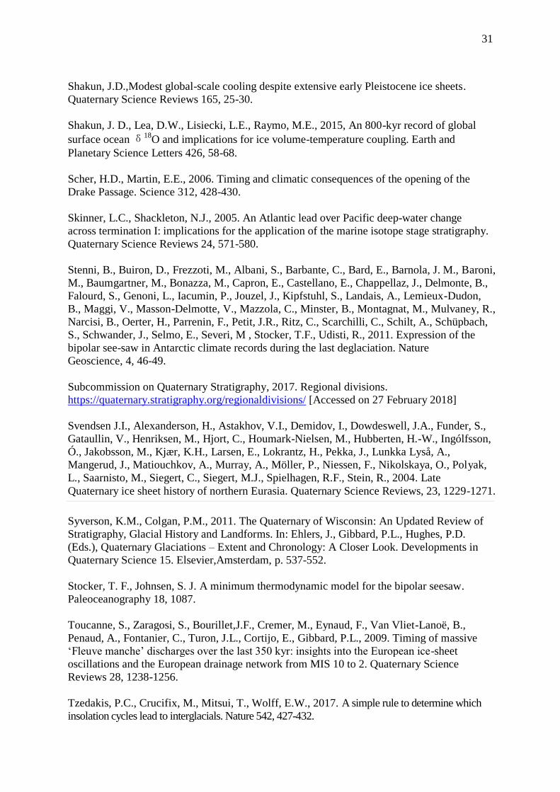
31

Shakun, J.D.,Modest global-scale cooling despite extensive early Pleistocene ice sheets.

Quaternary Science Reviews 165, 25-30.

Shakun, J. D., Lea, D.W., Lisiecki, L.E., Raymo, M.E., 2015, An 800-kyr record of global

surface ocean δ18O and implications for ice volume-temperature coupling. Earth and

Planetary Science Letters 426, 58-68.

Scher, H.D., Martin, E.E., 2006. Timing and climatic consequences of the opening of the

Drake Passage. Science 312, 428-430.

Skinner, L.C., Shackleton, N.J., 2005. An Atlantic lead over Pacific deep-water change

across termination I: implications for the application of the marine isotope stage stratigraphy.

Quaternary Science Reviews 24, 571-580.

Stenni, B., Buiron, D., Frezzoti, M., Albani, S., Barbante, C., Bard, E., Barnola, J. M., Baroni,

M., Baumgartner, M., Bonazza, M., Capron, E., Castellano, E., Chappellaz, J., Delmonte, B.,

Falourd, S., Genoni, L., Iacumin, P., Jouzel, J., Kipfstuhl, S., Landais, A., Lemieux-Dudon,

B., Maggi, V., Masson-Delmotte, V., Mazzola, C., Minster, B., Montagnat, M., Mulvaney, R.,

Narcisi, B., Oerter, H., Parrenin, F., Petit, J.R., Ritz, C., Scarchilli, C., Schilt, A., Schüpbach,

S., Schwander, J., Selmo, E., Severi, M , Stocker, T.F., Udisti, R., 2011. Expression of the

bipolar see-saw in Antarctic climate records during the last deglaciation. Nature

Geoscience, 4, 46-49.

Subcommission on Quaternary Stratigraphy, 2017. Regional divisions.

https://quaternary.stratigraphy.org/regionaldivisions/ [Accessed on 27 February 2018]

Svendsen J.I., Alexanderson, H., Astakhov, V.I., Demidov, I., Dowdeswell, J.A., Funder, S.,

Gataullin, V., Henriksen, M., Hjort, C., Houmark-Nielsen, M., Hubberten, H.-W., Ingólfsson,

Ó., Jakobsson, M., Kjær, K.H., Larsen, E., Lokrantz, H., Pekka, J., Lunkka Lyså, A.,

Mangerud, J., Matiouchkov, A., Murray, A., Möller, P., Niessen, F., Nikolskaya, O., Polyak,

L., Saarnisto, M., Siegert, C., Siegert, M.J., Spielhagen, R.F., Stein, R., 2004. Late

Quaternary ice sheet history of northern Eurasia. Quaternary Science Reviews, 23, 1229-1271.

Syverson, K.M., Colgan, P.M., 2011. The Quaternary of Wisconsin: An Updated Review of

Stratigraphy, Glacial History and Landforms. In: Ehlers, J., Gibbard, P.L., Hughes, P.D.

(Eds.), Quaternary Glaciations – Extent and Chronology: A Closer Look. Developments in

Quaternary Science 15. Elsevier,Amsterdam, p. 537-552.

Stocker, T. F., Johnsen, S. J. A minimum thermodynamic model for the bipolar seesaw.

Paleoceanography 18, 1087.

Toucanne, S., Zaragosi, S., Bourillet,J.F., Cremer, M., Eynaud, F., Van Vliet-Lanoë, B.,

Penaud, A., Fontanier, C., Turon, J.L., Cortijo, E., Gibbard, P.L., 2009. Timing of massive

‘Fleuve manche’ discharges over the last 350 kyr: insights into the European ice-sheet

oscillations and the European drainage network from MIS 10 to 2. Quaternary Science

Reviews 28, 1238-1256.

Tzedakis, P.C., Crucifix, M., Mitsui, T., Wolff, E.W., 2017. A simple rule to determine which

insolation cycles lead to interglacials. Nature 542, 427-432.

32

Van Andel, T.H., 2002. The climate and landscape of the Middle Part of the Weichselian

Glaciation in Europe: The Stage 3 project. Quaternary Research 57, 2-8.

Van Ginneken, M., Folco, L., Perchiazzi, N., Rochette, P., Bland, P.A., 2010. Meteoritic

ablation debris from the Transantarctic Mountains: Evidence for a Tunguska-like impact over

Antarctica ca. 480 ka ago. Earth and Planetary Science Letters 293, 104-113.

Velichko, A.A., Faustova, M.A., Gribchenko, Y.N., Pisareva, V.V., Sudakova, N.G., 2004.

Glaciations of the East European Plain – distribution and chronology. In: Ehlers, J., Gibbard,

P.L. (Eds.), Quaternary Glaciations – Extent and Chronology, Part I: Europe. Elsevier,

Amsterdam, p. 337-354.

Vorren, T.O., Landvik, J.Y., Andreassen, K., Laberg, J.S., 2011. Glacial History of the

Barents Sea Region. In: Ehlers, J., Gibbard, P.L., Hughes, P.D. (Eds.), Quaternary

Glaciations – Extent and Chronology: A Closer Look. Developments in Quaternary Science

15. Elsevier,Amsterdam, p. 362-372.

Waelbroeck, C., Labeyrie, L., Michel, E., Duplessy, J.C., McManus, J.F., Lambeck, K.,

Balbon, E., Labracherie, M., 2002. Sea-level and deep water temperature changes derived

from benthic foraminifera isotopic records. Quaternary Science Reviews 21, 295-305.

Walker, M.J.C., Johnsen, S., Rasmussen, S.O., Popp, T., Steffensen, J.-P., Gibbard, P.L,

Hoek,W., Andrews, J., Bj€ork, S., Cwynar, L.C., Hughen, K., Kershaw, P., Kromer, B., Litt,

T., Lowe, D.J., Nakagawa, T., Newnham, R., Schwander, J., 2009. Formal definition and

dating of the GSSP (Global Stratotype Section and Point) for the base of the Holocene using

the Greenland NGRIP ice core, and selected auxiliary records. Journal of Quaternary Science

24, 3-17.

White, T.S., Bridgland, D.R., Westaway, R., Straw, A., 2017. Evidence for a late Middle

Pleistocene glaciation of the British margin of the southern North Sea. Journal of Quaternary

Science 32, 261-275.

Zhou, S.Z., Wang, X.L., Wang, J., Xu, L.B., 2006. A preliminary study on timing of the

oldest Pleistocene glaciation in Qinghai–Tibetan Plateau. Quaternary International 154/155,

44-51.

33

Figures

Figure 1. Marine oxygen isotope stratigraphy from the Lisiecki and Raymo (2005) global

stack of 57 sediment cores. The stages are from Lisiecki and Raymo (2005) and the substages

beyond MIS 5e from Railsback et al. (2015).Terminations are indicated and the ages of these

are from Raymo (1997), Lisiecki and Raymo (2005) and Cheng et al. (2009). The lower

graph shows global sea surface temperature data from Shakun et al. (2015) which is derived

from a stack of 49 paired planktonic δ18

O-sea surface temperature (δ18

Op-SST) records from

the global oceans.

Figure 2A and B. The last ten glacial cycles (MIS 5d-2 to MIS 24-22) showing data over

these periods from i) the benthic δ18

O stack of Lisiecki and Raymo (2005), ii) dust flux from

the EPICA Dome C ice core record (Lambert et al. 2012), iii) temperature curves derived

from the EPICA Dome C ice core deuterium record (Jouzel et al. 2007b,c). The temperature

estimate in this curve is the estimated temperature difference over Antarctica compared with

the average of the past 1 ka, iv) insolation at 60°N from Berger and Loutre (1991) and Berger

(1992), v) CO2 data is from the Antarctic ice cores revised 800 ka CO2 data (Bereiter et al.

2015; NOAA 2018) .

Figure 3. Limits of the Eurasia contiguous ice sheets during the Middle and Late Pleistocene.

Adapted from information in Svendsen et al (2004), Ehlers and Gibbard (2004), and

Astakhov et al. (2016).

Figure 4. Benthic marine δ18

O isotope record (from Lisiecki and Raymo 2005) and solar

radiation at 60 and 30°N (full and dashed lines respectively; from Berger and Loutre 1991

and Berger 1992) for MIS 20 and 22-24. These intervals are beyond the ice core data records

used in Figure 2 and are therefore shown separately.

Figure 5. Regression between mean Northern Hemisphere Solar Radiation (at 60°N) and the

sea-levels detrended from the δ18

O record for the last eight glacial cycles using solar

radiation data from Berger and Loutre (1991) and Berger (1992) and detrended sea-level data

from Shakun et al. (2015). Figure a) is when defining glacials using the marine isotope stage

boundaries (i.e. MIS 5d-2, 6, 8, 10, 12, 14, 16, 18) whilst Figure b) is when defining glacial

cycles by Termination to Termination. In Figure b) MIS 14 is excluded from the regression

trendline calculation, The relationships are statistically significant for trendlines shown in a)

and b) where values of p = 0.0427 and 0.0440, respectively.

Figure 6. 50 ka moving average (black line) of δ18

O in the global stack (blue line) for

Lisiecki and Raymo (2005). The interval of 50 ka is chosen as this is half the theoretical 100

ka cycle. Increasing trends towards 100 ka cycles are illustrated by larger amplitudes in the

50 ka moving average of δ18

O values. The vertical black bold line marks the phase change

from subdued 100 ka cycles to larger amplitude 100 ka cycles from MIS 16 onwards.

34

Tables

Table 1. The definitions of the last ten full glacial cycles based on the marine isotope stratigraphy. 1) The boundaries of the glacial cycles are

defined by Termination ages provided in Raymo (1997), Lisiecki and Raymo (2005) and Cheng et al. (2009); 2) Cold ‘events’ are defined as

periods when the global sea surface temperatures (derived from global marine oxygen isotope records) were ≤0°C (Shakun et al. 2015). 3) The

numbering and span of the cold stages/substage intervals is based on Lisiecki and Raymo (2005) and Railsback et al. (2015). Detrended global

sea level values were obtained from Shakun et al. (2015).*Percentiles (5% and 25%, for δ18

O and sea-levels respectively) are based on the

glacial marine isotopic stage/substage subdivisions, definition 3) in this table.

Glacial cycles – definition in the marine

isotope records

1) Length of

glacial cycle

(termination

to

termination)

2) Cold

‘event’

length

3) Length of

“Cold Stage”

marine

isotopic

stage/substage

subdivisions

Maximum δ18

O

value

[corresponding

age]

Top 5% δ18

O

percentile*

Detrended

global sea-level

(m) – lower

quartile*

Basal

Termination

and age

Preceding

Interglacial

Stage/Substage

“Cold

Stage”

marine

isotope

stages

I [11.7 ka*]

II [130 ka] 5e 5d-2 118 57 103 5.02 [18 ka] 4.88 -83

IIIa [225

ka] 7a 6 95 54 61 4.98 [140 ka] 4.83 -115

III [243 ka] 9e 8 94 51 77 4.63 [252 ka] 4.53 -78

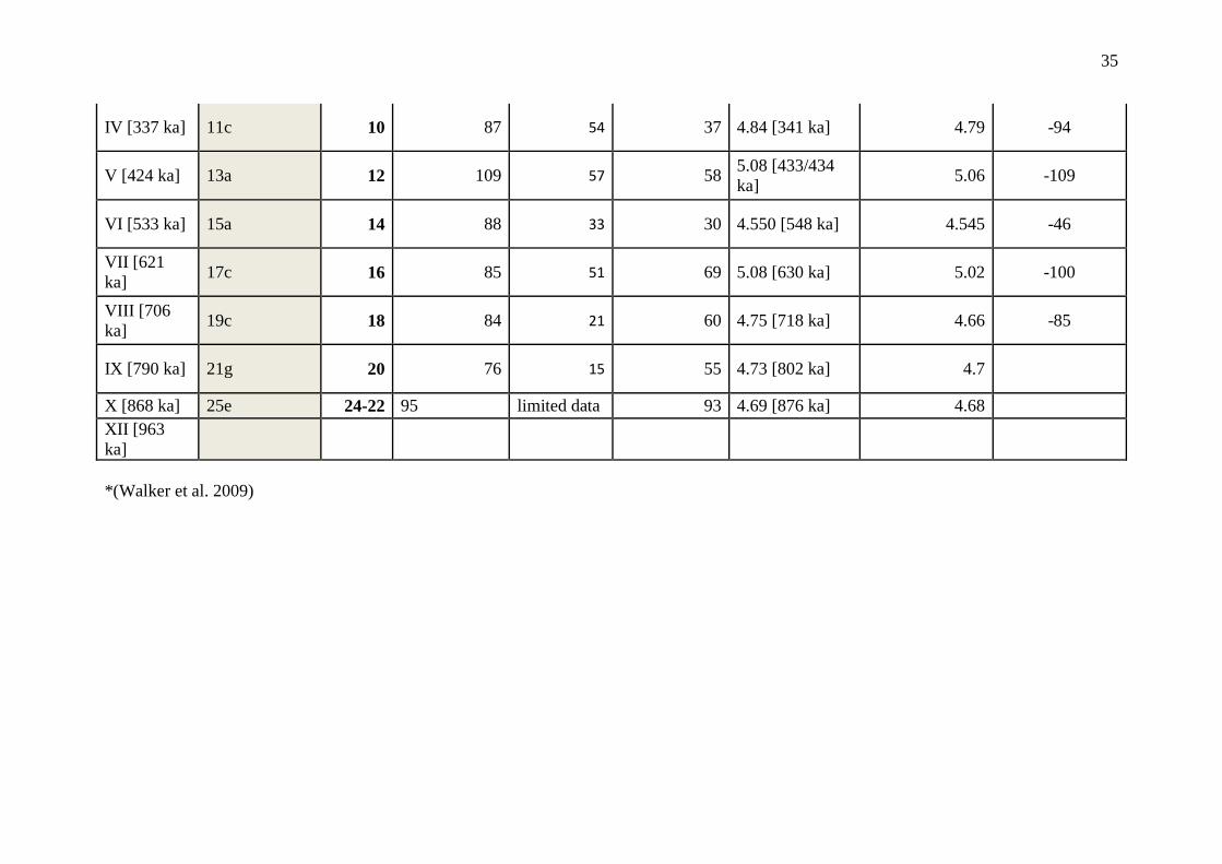
35

IV [337 ka] 11c 10 87 54 37 4.84 [341 ka] 4.79 -94

V [424 ka] 13a 12 109 57 58 5.08 [433/434

ka] 5.06 -109

VI [533 ka] 15a 14 88 33 30 4.550 [548 ka] 4.545 -46

VII [621

ka] 17c 16 85 51 69 5.08 [630 ka] 5.02 -100

VIII [706

ka] 19c 18 84 21 60 4.75 [718 ka] 4.66 -85

IX [790 ka] 21g 20 76 15 55 4.73 [802 ka] 4.7

X [868 ka] 25e 24-22 95 limited data 93 4.69 [876 ka] 4.68

XII [963

ka]

*(Walker et al. 2009)

36

Table 2. Solar radiation peak-trough amplitude at 60°N early in glacials or at the end of preceding interglacials. Solar radiation data is derived

from Berger and Loutre (1991) and Berger (1992) and marine isotope ages are from Lisiecki and Raymo (2005).

peak

age

(ka) trough

age

(ka)

amplitude

change

MIS 5e/5d-2 544.69 127 440.2 116 104.49

MIS 7/6 531.96 198 443 187 88.96

MIS 9/8 517.25 313 459.83 303 57.42

MIS 11/10 508.45 373 484.84 363 23.61

MIS 13/12 525.83 486 456.22 475 69.61

MIS 15/14 546.62 575 456.09 566 90.53

MIS 17/16 534.77 693 448.99 682 85.78

MIS 19/18 519.22 788 469.87 778 49.35

MIS 21/20 533.87 866 457.08 854 76.79

MIS 23/22 557.44 958 449.1 946 108.34

37

Figure 1

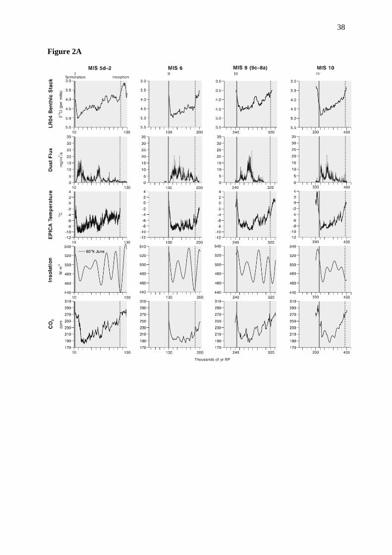
38

Figure 2A

39

Figure 2B (continued)

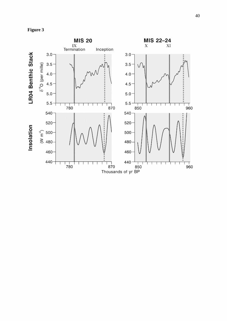
40

Figure 3

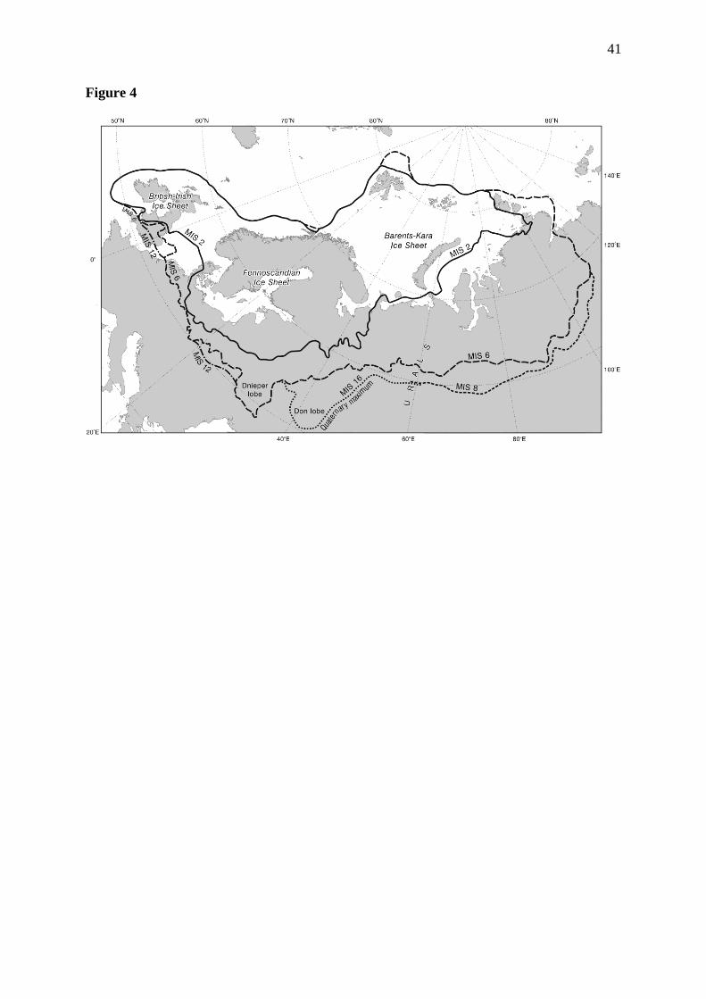
41

Figure 4

42

Figure 5

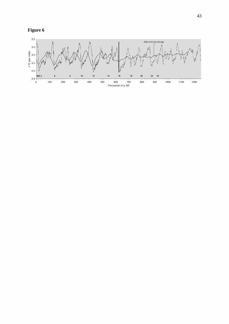
43

Figure 6