global food production and prices to 2050...global food production and prices to 2050 abares 1...
TRANSCRIPT
Global food production and prices to 2050
Scenario analysis under policy assumptions Verity Linehan, Sally Thorpe, Caroline Gunning-Trant,
Edwina Heyhoe, Kate Harle, Mary Hormis and Keely Harris-Adams
Research by the Australian Bureau of Agricultural
and Resource Economics and Sciences
Conference paper 13.6 March 2013
Paper presented at the 43rd ABARES Outlook conference 5–6 March 2013, Canberra, ACT

© Commonwealth of Australia 2013 Ownership of intellectual property rights Unless otherwise noted, copyright (and any other intellectual property rights, if any) in this publication is owned by the Commonwealth of Australia (referred to as the Commonwealth). Creative Commons licence All material in this publication is licensed under a Creative Commons Attribution 3.0 Australia Licence, save for content supplied by third parties, logos and the Commonwealth Coat of Arms.
Creative Commons Attribution 3.0 Australia Licence is a standard form licence agreement that allows you to copy, distribute, transmit and adapt this publication provided you attribute the work. A summary of the licence terms is available from creativecommons.org/licenses/by/3.0/au/deed.en. The full licence terms are available from creativecommons.org/licenses/by/3.0/au/legalcode.
This publication (and any material sourced from it) should be attributed as: Linehan, V, Thorpe, S, Gunning-Trant, C,
Heyhoe, E, Harle, K, Hormis, M & Harris-Adams, K 2013, Global food production and prices to 2050: scenario analysis under
policy assumptions, ABARES conference paper 13.6, Canberra, March. CC BY 3.0.
Cataloguing data Linehan, V, Thorpe, S, Gunning-Trant, C, Heyhoe, E, Harle, K, Hormis, M & Harris-Adams, K, Global food production and prices to 2050: scenario analysis under policy assumptions, ABARES conference paper 13.6, Canberra, March.
ISSN 1447-3666
ABARES project 43355
Internet
Global food production and prices to 2050 is available at daff.gov.au/abares/publications. Australian Bureau of Agricultural and Resource Economics and Sciences (ABARES) Postal address GPO Box 1563 Canberra ACT 2601 Switchboard +61 2 6272 2010| Facsimile +61 2 6272 2001 Email [email protected] Web daff.gov.au Inquiries regarding the licence and any use of this document should be sent to [email protected].
The Australian Government acting through the Department of Agriculture, Fisheries and Forestry represented by the
Australian Bureau of Agricultural and Resource Economics and Sciences, has exercised due care and skill in the preparation
and compilation of the information and data in this publication. Notwithstanding, the Department of Agriculture, Fisheries
and Forestry, ABARES, its employees and advisers disclaim all liability, including liability for negligence, for any loss,
damage, injury, expense or cost incurred by any person as a result of accessing, using or relying upon any of the information
or data in this publication to the maximum extent permitted by law.
Acknowledgements
The authors thank Neil Andrews and Jammie Penm for their insights during the project and for comments on the draft.
We also acknowledge sponsorship from Amcor Australasia, ANZ Banking Group Ltd, Cargill Australia Ltd, Coles, Elders Ltd,
Fisheries Research and Development Corporation, Grape and Wine Research and Development Corporation, Horticulture
Australia, the Northern Territory Department of Business, Queensland Department of Agriculture, Fisheries and Forestry,
Rural Industries Research and Development Corporation, Tasmanian Department of Economic Development, Tourism and
the Arts, Tasmanian Department of Primary Industries, Parks, Water and Environment, Victorian Department of Primary
Industries, the Western Australian Department of Agriculture and Food and the Australian Government Department of
Agriculture, Fisheries and Forestry.

Global food production and prices to 2050 ABARES
iii
Contents
Summary ............................................................................................................................................................ 1
1 Introduction .......................................................................................................................................... 3
2 Scenarios................................................................................................................................................. 5
Scenario 1: Establishing the reference scenario ..................................................................... 6
Scenario 2: Trade liberalisation with stronger productivity .......................................... 12
Scenario 3: Biofuels changes ........................................................................................................ 17
3 Conclusions ......................................................................................................................................... 21
Appendix A: ABARES agrifood model .................................................................................................. 23
Appendix B: Factors affecting future food production ................................................................. 27
Land availability ............................................................................................................................... 27
Productivity ........................................................................................................................................ 27
Appendix C: Sensitivity analysis ............................................................................................................ 30
Land productivity assumptions .................................................................................................. 30
Total factor productivity assumptions .................................................................................... 32
Land availability assumptions .................................................................................................... 33
References ...................................................................................................................................................... 35
Tables
Table 1 Reference scenario—annual average land productivity growth rates, by region and commodity group, from 2007 to 2050 ........................................................... 7
Table 2 Higher rainfall deficiency—annual average land productivity growth, by region and commodity group, from 2007 to 2050 ........................................................ 11
Table 3 Biofuel simulations: real world prices for maize and rapeseed, change from 2007 to 2050 ........................................................................................................... 19
Table A1 Commodities in the ABARES agrifood model ................................................................ 24
Table A2 Regions in the ABARES agrifood model ........................................................................... 25
Table A3 Average annual real income growth, 2007 to 2050 .................................................... 25
Table A4 Arable land projected change, 2005–07 to 2050 ......................................................... 26
Table C1 Sensitivity analysis, change from 2007 to 2050 ........................................................... 30
Figures
Figure 1 Reference scenario—world real price, change from 2007 to 2050 .......................... 7
Figure 2 Reference scenario—real value of world agrifood production, by region, 2007 and 2050 ................................................................................................................ 8
Global food production and prices to 2050 ABARES
iv
Figure 3 Reference scenario—real value of world agrifood consumption, by region, 2007 and 2050 ................................................................................................................ 9
Figure 4 Reference scenario—real value of world agrifood production, by commodity group, 2007 and 2050 ......................................................................................... 9
Figure 5 Reference scenario—real value of Asian agrifood imports, by commodity group, 2007 and 2050 ...................................................................................... 10
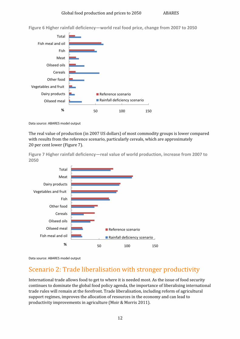
Figure 6 Higher rainfall deficiency—world real food price, change from 2007 to 2050 ........................................................................................................... 12
Figure 7 Higher rainfall deficiency—real value of world production, increase from 2007 to 2050 ......................................................................................................... 12
Figure 8 Trade liberalisation scenario—world real food price, change from 2007 to 2050 ........................................................................................................... 14
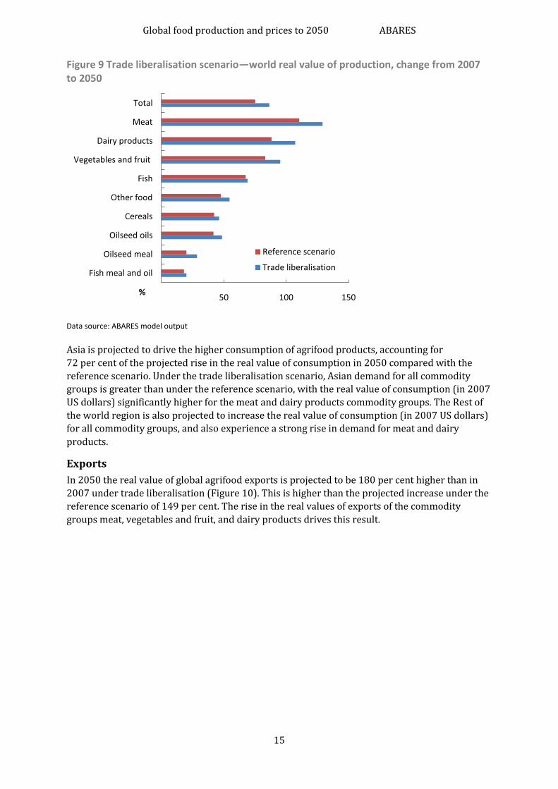
Figure 9 Trade liberalisation scenario—world real value of production, change from 2007 to 2050 ........................................................................................................... 15
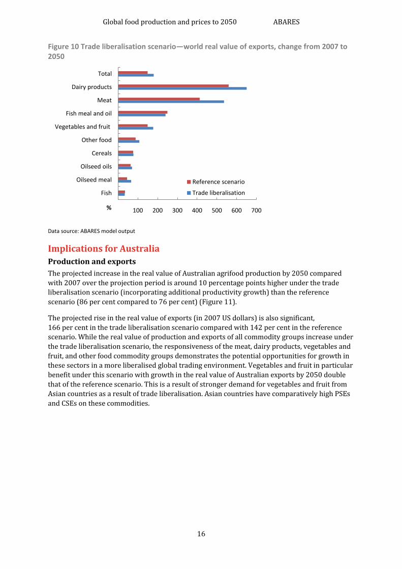
Figure 10 Trade liberalisation scenario—world real value of exports, change from 2007 to 2050 ........................................................................................................... 16
Figure 11 Trade liberalisation scenario—Australian real value of production, change from 2007 to 2050 ........................................................................................................... 17
Figure B1 Global capture and aquaculture fisheries production, 1950–2010 .................... 28
Figure C1 Land productivity sensitivity—world real food, change from 2007 to 2050 ........................................................................................................... 31
Figure C2 Land productivity sensitivity—world real value of production under high and low land productivity growth, change from 2007 to 2050 ........................... 31
Figure C3 Total factor productivity sensitivity—world real price, change from 2007 to 2050 ........................................................................................................... 32
Figure C4 Total factor productivity sensitivity—world real value, change from 2007 to 2050 ........................................................................................................... 33
Figure C5 Land availability sensitivity—world real price, change from 2007 to 2050 ........................................................................................................... 34
Figure C6 Land availability sensitivity—world real value of production under higher and lower land availability, change from 2007 from 2050 ............................... 34
Global food production and prices to 2050 ABARES
1
Summary With food security at the forefront of government policy agendas worldwide, much of the focus
is on how the world will respond to a rise in food demand over the next 40 years. Many
institutions, including the Food and Agriculture Organization of the United Nations (FAO), the
International Food Policy Research Institute (IFPRI) and ABARES, have published projections of
an increase in global food demand out to 2050.
This report uses three scenarios to investigate the possible response of world food prices, food
production and trade to the projected increase in demand. This work builds on agrifood
modelling in ABARES Food demand to 2050: Opportunities for Australian agriculture (Linehan et
al. 2012a).
The uncertainties and dynamics surrounding factors such as climate change, international trade
policy and biofuels policies add to the complexity of modelling global agrifood markets out to
2050. However, scenario analysis, which isolates each of these issues, allows for an assessment
of indicative price and production responses over the projection period across different regions
and agrifood commodities. A reference scenario is developed for this project using a set of
assumptions drawn from the literature. The reference scenario serves as a starting point for the
policy analysis and shows the sensitivity of the projections to changes in assumptions and
parameter values.
This report uses an updated version of the ABARES agrifood model (Linehan et al. 2012b) that
includes new assumptions about agricultural productivity growth, land availability and fisheries.
Projections of global supply and price responses of agrifood products (food-based agricultural
commodities and fish) are derived from a partial equilibrium model of agricultural markets that
ABARES developed for this purpose. ABARES used the model to prepare projections that
consistently account for the main economic forces linking demand and supply for various food
commodities within a region and between regions over time.
In the reference scenario, the average price of world agrifood products in 2050 is projected to be
11.5 per cent higher than in 2007. However, it should be noted that prices have already risen
considerably since 2007 and the price projections in this paper represent a marginal increase
from 2012 average prices. The fish meal and oil, fish, meat, oilseed oils, and cereals commodity
groups experience the largest price rise over the projection period. Associated with these price
increases is a 75 per cent rise in the projected real value of world agrifood production and
consumption over the same period. Most of the projected rise in food production occurs in Asia,
where the real value of agrifood production is 84 per cent higher in 2050 than in 2007 (in 2007
US dollars). China accounts for over half the projected increase in the real value of Asian
agrifood production, particularly from the meat, dairy products, fish, and vegetables and fruit
commodity groups.
To compare the implications of alternative policy assumptions relating to food production, two
additional scenarios are included in this report. The first policy scenario examines the response
of world agrifood markets to more liberalised agrifood trade with trade liberalisation assumed
to lead to additional productivity growth. Under this scenario, world agrifood prices rise
10.4 per cent between 2007 and 2050 (in 2007 US dollars). This projected price increase is not
as strong as the reference scenario (when agricultural trade is protected) because of the
assumed higher productivity growth induced by trade liberalisation. Liberalised trade also leads
to a stronger rise in the real value of global agrifood exports between 2007 and 2050 compared
Global food production and prices to 2050 ABARES
2
with the reference scenario (180 per cent rather than 149 per cent) as open markets allow an
expansion of global trade.
The second scenario examines the response of world markets to a reduction in food grains in the
production of biofuels in the United States and the European Union. When maize is completely
removed from the production of US and rapeseed from the production of EU biofuels, the world
price of maize falls in 2050 relative to 2007 as the competition for maize between the livestock,
food and energy sectors is reduced. Rapeseed prices in 2050 are significantly higher than 2007
(in 2007 US dollars) reflecting the continued projected strength of demand for rapeseed for both
food and feed use.
Projected increases in Australian agricultural production and exports reflect the commodities
where Australia has a comparative advantage. Australia needs to remain competitive to meet the
opportunities provided by higher global agrifood demand. Land and water constraints are
inherent in Australian agriculture. If Australia is to remain responsive to changes in world
agrifood markets and provide those foods most in demand in expanding markets, it will have to
maintain productivity growth through ongoing investment in research and development.
Sensitivity analysis around some of the underlying assumptions, including land productivity,
total factor productivity (TFP) and land availability, was undertaken to examine the robustness
of the model and to gauge the response of global food price movements to the supply
constraints. This analysis illustrated the significant impact of an increase in TFP growth in
increasing food production and reducing upward pressure on global food prices. This result
highlights the importance of improvements in productivity to meet the global food security
challenge toward 2050.
Australia is well located to take advantage of the opportunities that higher food consumption
will provide but there will be a need for a change to agricultural production in Australia to fully
capture these opportunities. This will only be accomplished with a reversal of the recent slowing
rate of growth in productivity and more targeting of consumer needs in the growth areas of the
world—particularly Asia. At the industry level, this will require greater targeting of our products
to more diversified markets and targeting different qualities of our products to market segments
where there is greatest potential for value adding. Higher prices can lead to higher productivity
by improving incentives for investment in research and development, through innovation and
through adaptation of existing overseas technologies applied to an Australian environment. The
government can also assist through a strong commitment to furthering global trade
liberalisation and increasing access to a diverse range of overseas markets. Governments will
need to continue to provide a sound economic environment, with appropriate fiscal policy
settings that encourage economic and productivity growth—goals achievable only if regulation
is limited to those areas where market failures exist and where the benefits of regulation clearly
outweigh its costs.
Global food production and prices to 2050 ABARES
3
1 Introduction By 2050 world demand for agrifood products is projected to increase significantly because of a
larger global population and growth in per person incomes, especially in developing countries.
How agricultural production and trade will respond to this increase in demand over the next 40
years will depend on changes in economic, political, environmental and technological factors.
Climate change, soil and water degradation, and land availability are some factors that
agricultural producers will have to increasingly contend with if they are to maintain or improve
levels of agricultural productivity.
In the report Food demand to 2050: Opportunities for Australian agriculture (Linehan et al.
2012a), ABARES projected the real value (in 2007 US dollars) of world agrifood demand to be
77 per cent higher in 2050 than in 2007 (Linehan et al. 2012a). This represents an annual
average increase of 1.3 per cent over this period. Demand is projected to increase most strongly
in Asia, doubling between 2007 and 2050. China is driving this demand, accounting for
43 per cent of the global agrifood increase, while India accounts for 13 per cent (Linehan et al.
2012a).
In this earlier report, the food products projected to be most sought after by 2050 were found to
be the vegetables and fruit, meat, dairy products, cereals and fish commodity groups (Linehan et
al. 2012a). China accounts for much of the projected increase in world import demand for these
products, while the growth in demand from India was projected to be strongest for dairy
products. These results are consistent with the expected change in diets toward high value
products as consumer incomes rise.
The projected increase in global demand for agrifood products will affect global agricultural
prices going forward. Several factors may influence production, consumption and prices over
this period; for example, resource constraints are likely to affect productivity growth.
Government policies, such as those relating to trade and biofuels, will also influence prices.
With food security at the forefront of many governments’ policy agendas, the objective of this
report is to highlight possible indicative price changes and production responses in 2050
compared with 2007 across a number of supply-side scenarios. These scenarios reflect possible
constraints and challenges that producers of agrifood commodities around the world will likely
face, including land availability, rainfall deficiency, and trade and biofuel policy changes.
Scenario analysis has been utilised in this report to examine the implications of alternative
assumptions relating to food production. The procedure involves establishing a reference
scenario with future prices, production, consumption and trade under a set of specified
economic and environmental assumptions. The outcome of each scenario, in which some of the
key underlying assumptions are altered, is then compared against the reference scenario.
The price projections toward 2050 presented in the reference scenario are conditional on the
underlying assumptions. Those assumptions were sourced mainly from recent studies and
should not be interpreted as ABARES long-term projections.
An updated version of the ABARES agrifood model (Linehan et al. 2012b) was used for this
analysis. This model is an economic simulation model of global agricultural supply, demand and
trade. The model was used to prepare annual projections between 2007 and 2050, and has been
updated to include a set of supply-side assumptions relating to, for example productivity growth
(Rosenzweig et al. 2012), availability of arable land (Alexandratos & Bruinsma 2012) and
Global food production and prices to 2050 ABARES
4
expectations about growth in global fisheries (FAO 2012). These projections are based on
assumptions, data and projections from FAO and Agricultural Modelling Intercomparison and
Improvement Project (AgMIP).
The projections are also conditional on parameter values used to represent the sensitivities of
food demand and supply to economic forces. Changes to these assumptions and parameters
have resulted in adjustments to the projections originally reported in Linehan and colleagues
(2012a).
The commodity and regional coverage in the ABARES agrifood model provides projections for
Australia and other major world agricultural exporters and importers. In addition, the best
practice mixed complementarity framework (Rutherford 1995) is adopted to model key
activities in production and policy, and impose key resource limits on land use, fish catch and
yield growth (Linehan et al. 2012b).
Global food production and prices to 2050 ABARES
5
2 Scenarios The objective of using scenario analysis for this report is to examine the implications of
alternative resource availability and policy assumptions relating to food production. Three
scenarios are used:
Scenario 1: Establishing the reference scenario
Scenario 2: Trade liberalisation with stronger productivity
Scenario 3: Biofuels changes.
The outcomes of scenarios 2 and 3, in which some key underlying assumptions are altered, are
compared against the reference projection in Scenario 1.
Scenario 1 establishes a reference scenario. It is in this scenario that parameter values used in
Food demand to 2050: Opportunities for Australian agriculture (Linehan et al. 2012a) are updated
using the latest information from FAO and AgMIP (Appendix A). The scenario incorporates
important assumptions about:
projected land availability toward 2050, across all regions in the model
land productivity growth rates
rainfall deficiency (reflected in land productivity growth for crops)
growth in global fisheries production.
The objective of this scenario is to provide a more comprehensive assessment of the response of
agrifood markets to the projected increase in global demand reported in Linehan and colleagues
(2012a).
Scenarios 2 and 3 build on the reference scenario by imposing stylised assumptions relating to
trade liberalisation and biofuels developments on the model. The projections for world agrifood
prices, production and trade emanating from these scenarios are indicative only, but are useful
as a basis of comparison to understand the possible market adjustments that could take place
under significant policy changes.
Scenario 2 considers trade liberalisation, where producer and consumer support, as measured
by the OECD producer and consumer support estimates, are removed. At the same time, it is
assumed that TFP (which is broadly defined as output divided by total inputs) will increase over
some of the projection period as more liberalised trade allows, among other things, quicker
technological catch-up of developing countries and greater investment in agriculture. The
objective of this scenario is to better understand the nature of adjustment of global agrifood
markets, relative to the reference scenario, when food products are allowed to flow more freely
between countries and regions. The trade response of Australia is of specific interest given its
geographic proximity to Asia, where a significant increase in agrifood demand is projected
(Linehan et al. 2012a).
Scenario 3 considers a reduction in the amount of maize and rapeseed used in the production of
biofuels in the United States and European Union, respectively. The objective of the scenario is
to understand the sensitivity of world cereal markets to a progressive decline in the supply of
Global food production and prices to 2050 ABARES
6
maize and rapeseed for biofuel production. Given the substitutability of grains in feed use, the
impact on the production and export of wheat and canola in Australia is of particular interest.
Scenario 1: Establishing the reference scenario
Productivity growth assumptions
Productivity growth is an important determinant of long-run agricultural production. However,
determining future rates of productivity growth is challenging given the uncertain nature of
future technological advancement and the potential influence of changes in the natural resource
base arising from climate change and other factors. The reference scenario simulated in this
analysis assumes present climate conditions are maintained to 2050 and productivity is driven
by technological changes alone. For comparative purposes, a rainfall deficiency scenario is also
presented which incorporates analysis of the effects of rainfall deficiency on the land
productivity of cropping.
The rate of technological progress has been a key driver of productivity growth in the past. One
example of a technological progress is the development of crop varieties with higher yields. By
contrast, technical efficiency reflects, for example, the adoption of existing technologies in order
to catch up. Improvements in technical efficiency are potentially important determinants of
productivity growth rates in developing countries.
The capacity of the natural resource base to accommodate increasing agricultural production is
the subject of ongoing debate. Water availability, diminishing soil quality and desertification
have been identified as potential causes of declining productivity growth rates into the future
(Appendix B). At the same time, climate change is projected to increasingly influence agricultural
productivity; however, depending on the region, the effects for individual regions and
commodities could be for better or for worse (IPCC 2007).
The two types of productivity improvements in the ABARES agrifood model are land
productivity and TFP improvements. Improvements in land productivity reflect a reduction in
the input of land per unit of output of cropping or livestock product. This is a partial measure of
productivity, where a single factor, land, experiences technological advancement. TFP is a
measure of the value of total output relative to the value of total inputs.
Crop land productivity growth estimates for this study stem from the AgMIP model comparison
exercise (Table 1). Land productivity growth assumptions out to 2050 are driven by technology
improvements, including crop management research, conventional plant breeding and other
more advanced breeding techniques. Other sources of land productivity growth incorporated in
the estimates include private sector agricultural research and development, agricultural
extension and education, the development of markets, improved infrastructure, availability of
irrigation, and access to water.
Livestock land productivity estimates used in the model are derived from the ABARES Global
Trade and Environment model (GTEM), a multisector, multiregion dynamic global computable
general equilibrium model of the world economy (ABARE 2007).
In general, productivity growth is projected to be higher for livestock-based industries than for
cropping (Table 1) and highest for livestock products in China and India.
Global food production and prices to 2050 ABARES
7
Table 1 Reference scenario—annual average land productivity growth rates, by region and commodity group, from 2007 to 2050
Food group World (%)
Australiaa
(%)
China (%)
India (%)
Rest of Asia (%)
Rest of world (%)
Meat 1.6 1.3 2.3 3.0 1.6 1.6 Dairy products 1.6 1.3 2.3 3.0 1.6 1.6 Cereals 1.3 1.2 1.1 1.2 1.3 1.4 Other food 1.0 0.8 1.2 1.1 0.9 1.0 Vegetables and fruit 0.8 0.7 0.6 0.9 0.6 0.9
a Australia is also part of the Rest of world region.
Data sources: Agricultural Modelling Intercomparison and Improvement Project; ABARES Global Trade and Environment
model
Productivity projections used in this study are broadly consistent with OECD/FAO (2012)
2001-40 projections. The OECD/FAO (2012) project the world average TFP to be 1.38 per cent a
year from 2001 to 2040, with ABARES world average TFP projection approximately 1 per cent a
year from 2007 to 2050.
Results from the reference scenario
Given the productivity assumptions set out above, the real value of world agrifood production
and consumption in 2050 (in 2007 US dollars) is projected to be 75 per cent higher than in 2007,
with real prices (in 2007 US dollars) projected to increase, on average, by 11.5 per cent over this
period (Figure 1). By comparison, the FAO real food price index rose by 10.8 per cent between
2007 and 2012 due mainly to droughts in some major producing countries (FAO 2013). Using
recent movements in food prices as a guide, the simulation results indicate that food prices (in
real terms) by 2050 are projected to be only marginally higher than their average in 2012.
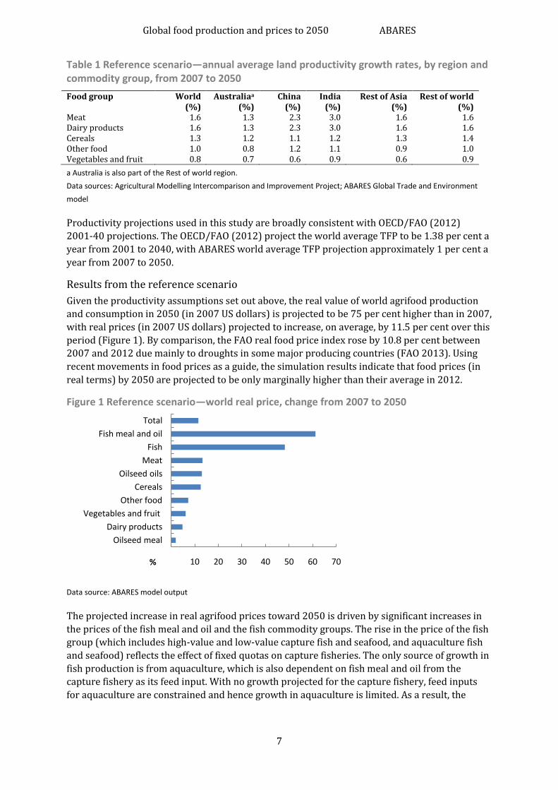
Figure 1 Reference scenario—world real price, change from 2007 to 2050
Data source: ABARES model output
The projected increase in real agrifood prices toward 2050 is driven by significant increases in
the prices of the fish meal and oil and the fish commodity groups. The rise in the price of the fish
group (which includes high-value and low-value capture fish and seafood, and aquaculture fish
and seafood) reflects the effect of fixed quotas on capture fisheries. The only source of growth in
fish production is from aquaculture, which is also dependent on fish meal and oil from the
capture fishery as its feed input. With no growth projected for the capture fishery, feed inputs
for aquaculture are constrained and hence growth in aquaculture is limited. As a result, the
10 20 30 40 50 60 70
Oilseed meal
Dairy products
Vegetables and fruit
Other food
Cereals
Oilseed oils
Meat
Fish
Fish meal and oil
Total
%
Global food production and prices to 2050 ABARES
8
prices of all types of fish rise significantly toward 2050. Appendix B provides background on
world fisheries.
The next largest price increases over the projection period are in the meat (13.3 per cent),
oilseed oils (13.0 per cent) and cereals (12.5 per cent) commodity groups.
It is projected that developing countries will be the main source of global agrifood production
growth to 2050, as they have a greater potential to increase agricultural land and improve
productivity. By 2050 developing countries’ share of global agrifood production is projected to
increase to 74.3 per cent from 70.3 per cent in 2007.
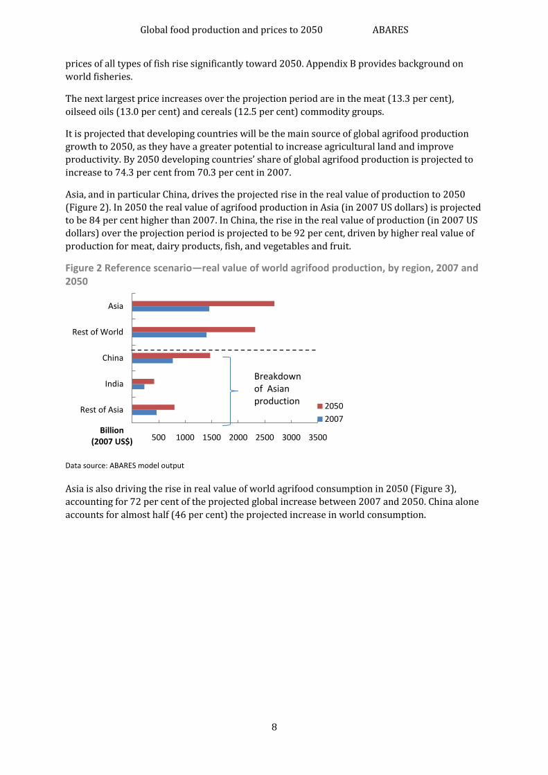
Asia, and in particular China, drives the projected rise in the real value of production to 2050
(Figure 2). In 2050 the real value of agrifood production in Asia (in 2007 US dollars) is projected
to be 84 per cent higher than 2007. In China, the rise in the real value of production (in 2007 US
dollars) over the projection period is projected to be 92 per cent, driven by higher real value of
production for meat, dairy products, fish, and vegetables and fruit.
Figure 2 Reference scenario—real value of world agrifood production, by region, 2007 and 2050
Data source: ABARES model output
Asia is also driving the rise in real value of world agrifood consumption in 2050 (Figure 3),
accounting for 72 per cent of the projected global increase between 2007 and 2050. China alone
accounts for almost half (46 per cent) the projected increase in world consumption.
500 1000 1500 2000 2500 3000 3500
Rest of Asia
India
China
Rest of World
Asia
Billion (2007 US$)
2050
2007
Breakdown of Asian production

Global food production and prices to 2050 ABARES
9
Figure 3 Reference scenario—real value of world agrifood consumption, by region, 2007 and 2050
Data source: ABARES model output
In terms of commodity groups, the largest increases in the real value of global agrifood
production (in US 2007 dollars) in the reference scenario are for vegetables and fruit and meat
(Figure 4). The vegetables and fruit group accounts for 44 per cent of the projected rise in the
real value of agrifood production (in US 2007 dollars), while meat accounts for 26 per cent. In
terms of annual average growth, the groups that are expected to grow fastest between 2007 and
2050 are meat (1.7 per cent a year), dairy products (1.5 per cent) and fish (1.2 per cent).
Figure 4 Reference scenario—real value of world agrifood production, by commodity group, 2007 and 2050
Data source: ABARES model output
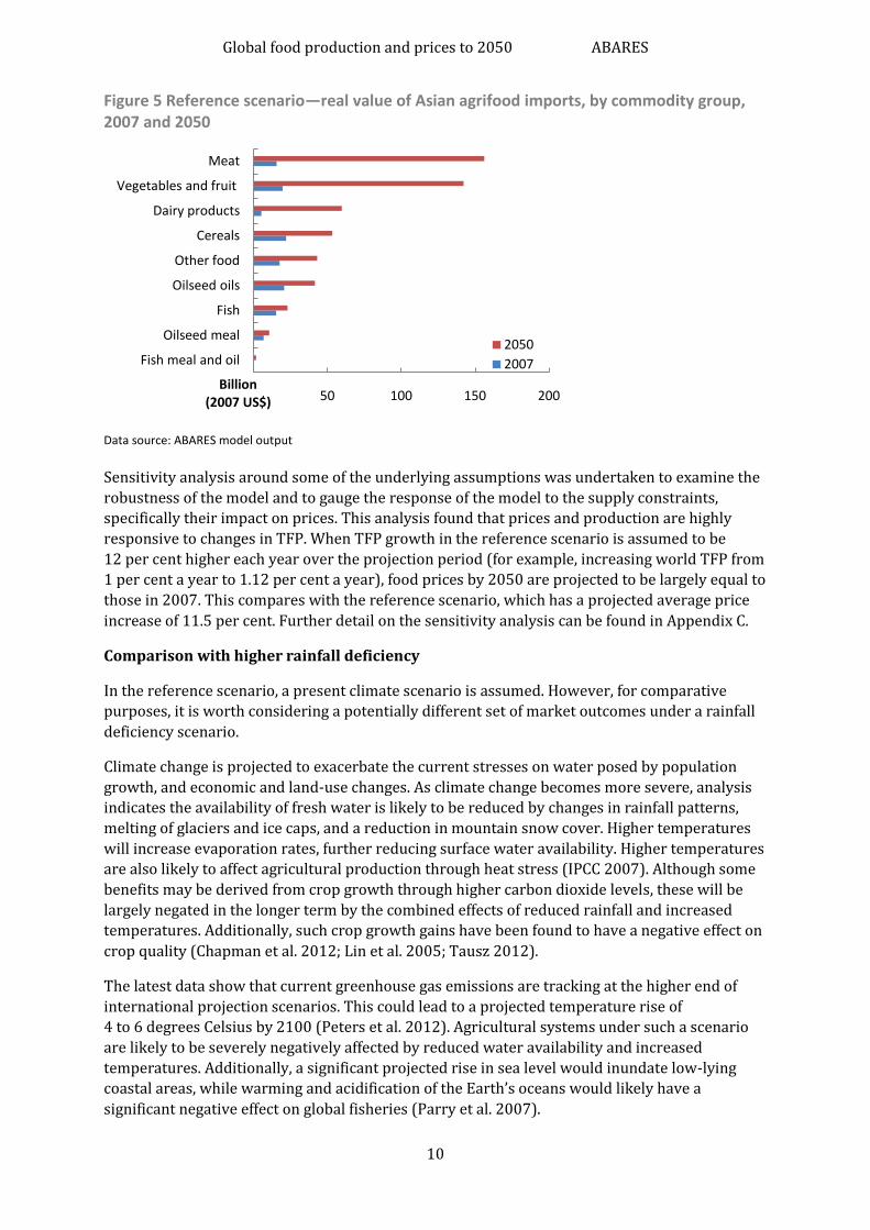
The real value of world agrifood imports is projected to increase from US$278 billion in 2007 to
US$694 in 2050 (in 2007 US dollars), a rise of 149 per cent (or 2.1 per cent annually). Asia
accounts for the bulk of the growth in agrifood imports, with China driving most of this rise.
Asia’s import position is driven by substantial increases in imports of meat and vegetables and
fruit (Figure 5).
500 1000 1500 2000 2500 3000 3500
Rest of Asia
India
China
Rest of World
Asia
Billion (2007 US$)
2050
2007
Breakdown of Asian consumption
500 1000 1500 2000 2500
Fish meal and oil
Oilseed meal
Oilseed oils
Other food
Fish
Dairy products
Cereals
Meat
Vegetables and fruit
Billion (2007 US$)
2050
2007
Global food production and prices to 2050 ABARES
10
Figure 5 Reference scenario—real value of Asian agrifood imports, by commodity group, 2007 and 2050
Data source: ABARES model output
Sensitivity analysis around some of the underlying assumptions was undertaken to examine the
robustness of the model and to gauge the response of the model to the supply constraints,
specifically their impact on prices. This analysis found that prices and production are highly
responsive to changes in TFP. When TFP growth in the reference scenario is assumed to be
12 per cent higher each year over the projection period (for example, increasing world TFP from
1 per cent a year to 1.12 per cent a year), food prices by 2050 are projected to be largely equal to
those in 2007. This compares with the reference scenario, which has a projected average price
increase of 11.5 per cent. Further detail on the sensitivity analysis can be found in Appendix C.
Comparison with higher rainfall deficiency
In the reference scenario, a present climate scenario is assumed. However, for comparative
purposes, it is worth considering a potentially different set of market outcomes under a rainfall
deficiency scenario.
Climate change is projected to exacerbate the current stresses on water posed by population
growth, and economic and land-use changes. As climate change becomes more severe, analysis
indicates the availability of fresh water is likely to be reduced by changes in rainfall patterns,
melting of glaciers and ice caps, and a reduction in mountain snow cover. Higher temperatures
will increase evaporation rates, further reducing surface water availability. Higher temperatures
are also likely to affect agricultural production through heat stress (IPCC 2007). Although some
benefits may be derived from crop growth through higher carbon dioxide levels, these will be
largely negated in the longer term by the combined effects of reduced rainfall and increased
temperatures. Additionally, such crop growth gains have been found to have a negative effect on
crop quality (Chapman et al. 2012; Lin et al. 2005; Tausz 2012).
The latest data show that current greenhouse gas emissions are tracking at the higher end of
international projection scenarios. This could lead to a projected temperature rise of
4 to 6 degrees Celsius by 2100 (Peters et al. 2012). Agricultural systems under such a scenario
are likely to be severely negatively affected by reduced water availability and increased
temperatures. Additionally, a significant projected rise in sea level would inundate low-lying
coastal areas, while warming and acidification of the Earth’s oceans would likely have a
significant negative effect on global fisheries (Parry et al. 2007).
50 100 150 200
Fish meal and oil
Oilseed meal
Fish
Oilseed oils
Other food
Cereals
Dairy products
Vegetables and fruit
Meat
Billion (2007 US$)
2050
2007
Global food production and prices to 2050 ABARES
11
To compare the effect of a severe, climate-induced reduction to land productivity with the
reference scenario results, a second set of crop productivity assumptions from the AgMIP
climate scenario set was used in the agrifood model. Under this scenario, projected land
productivity growth rates are modified to reflect the highest greenhouse gas emissions scenario
modelled by the Intergovernmental Panel on Climate Change (IPCC) (Rosenzweig et al. 2012).
The crop productivity implications of these concentration levels were modelled using a global
climate (IPSL-CM5A-LR) and crop model (DSSAT) combination. The climate model projects
changes in temperature and rainfall arising from increased greenhouse gas concentrations, and
the crop model translates these changes in climate into changes in crop productivity.
Livestock productivity estimates remain unchanged from the reference scenario. However,
livestock commodities will be impacted by this scenario due to higher feed costs resulting from
lower productivity of crops. Fish productivity estimates are also unchanged, and climate change
is assumed to have little impact on fish under this scenario.
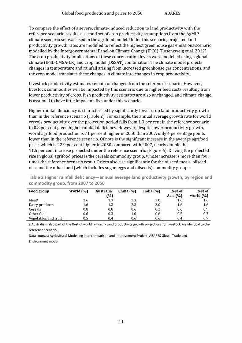
Higher rainfall deficiency is characterised by significantly lower crop land productivity growth
than in the reference scenario (Table 2). For example, the annual average growth rate for world
cereals productivity over the projection period falls from 1.3 per cent in the reference scenario
to 0.8 per cent given higher rainfall deficiency. However, despite lower productivity growth,
world agrifood production is 71 per cent higher in 2050 than 2007, only 4 percentage points
lower than in the reference scenario. Of note is the significant increase in the average agrifood
price, which is 22.9 per cent higher in 2050 compared with 2007, nearly double the
11.5 per cent increase projected under the reference scenario (Figure 6). Driving the projected
rise in global agrifood prices is the cereals commodity group, whose increase is more than four
times the reference scenario result. Prices also rise significantly for the oilseed meals, oilseed
oils, and the other food (which includes sugar, eggs and oilseeds) commodity groups.
Table 2 Higher rainfall deficiency—annual average land productivity growth, by region and commodity group, from 2007 to 2050
Food group World (%) Australiaa (%)
China (%) India (%) Rest of Asia (%)
Rest of world (%)
Meatb 1.6 1.3 2.3 3.0 1.6 1.6 Dairy products 1.6 1.3 2.3 3.0 1.6 1.6 Cereals 0.8 0.8 0.6 0.2 0.6 0.9 Other food 0.6 0.3 1.0 0.6 0.5 0.7 Vegetables and fruit 0.5 0.4 0.6 0.6 0.4 0.7
a Australia is also part of the Rest of world region. b Land productivity growth projections for livestock are identical to the
reference scenario.
Data sources: Agricultural Modelling Intercomparison and Improvement Project; ABARES Global Trade and
Environment model
Global food production and prices to 2050 ABARES
12
Figure 6 Higher rainfall deficiency—world real food price, change from 2007 to 2050
Data source: ABARES model output
The real value of production (in 2007 US dollars) of most commodity groups is lower compared
with results from the reference scenario, particularly cereals, which are approximately
20 per cent lower (Figure 7).
Figure 7 Higher rainfall deficiency—real value of world production, increase from 2007 to 2050
Data source: ABARES model output
Scenario 2: Trade liberalisation with stronger productivity
International trade allows food to get to where it is needed most. As the issue of food security
continues to dominate the global food policy agenda, the importance of liberalising international
trade rules will remain at the forefront. Trade liberalisation, including reform of agricultural
support regimes, improves the allocation of resources in the economy and can lead to
productivity improvements in agriculture (Moir & Morris 2011).
50 100 150
Oilseed meal
Dairy products
Vegetables and fruit
Other food
Cereals
Oilseed oils
Meat
Fish
Fish meal and oil
Total
%
Reference scenario
Rainfall deficiency scenario
50 100 150
Fish meal and oil
Oilseed meal
Oilseed oils
Cereals
Other food
Fish
Vegetables and fruit
Dairy products
Meat
Total
%
Reference scenario
Rainfall deficiency scenario
Global food production and prices to 2050 ABARES
13
Over the past four decades there have been significant developments in agricultural trade and in
the policies and institutions surrounding it (Josling 2008). In recent years there has been a shift
toward regional and bilateral trade agreements, while multilateral negotiations have stalled.
Continued integration through these regional and bilateral agreements and continued support
for the World Trade Organization (WTO) will affect trade liberalisation in coming years.
The short-term outlook for trade liberalisation is uncertain and is dependent on many factors,
including global economic growth, growth in agricultural output and investment and continued
policy reform in developed and developing countries (Josling 2008; Sarris 2009). Price volatility
and absolute price levels may also affect the direction of agricultural trade policy. An example of
this type of response occurred as recently as 2008 when high and volatile food prices led some
countries to impose restrictions on exports.
Trade liberalisation with stronger productivity scenario
While it is not possible to accurately predict the path of trade liberalisation out to 2050, it is
worth examining the effects of one possible trade liberalisation scenario and its price
implications. This scenario utilises heavily stylised policy settings and assumptions with the aim
of providing an indication of the world agrifood price response.
In the model a price wedge approach is used to take into account the difference between
domestic producer and consumer prices and the world price, where the producer price is
defined as the domestic market price inflated by the exogenous ad valorem producer support
estimate (PSE), while the consumer price is the domestic price deflated by the exogenous ad
valorem consumer support estimate (CSE). This price wedge approach is frequently used in
trade liberalisation modelling; for example, by IFPRI, using the IMPACT model, and by ABARES.
For further information on PSEs and CSEs see the OECD Producer and Consumer Support
Estimates database (OECD 2013).
Economic theory suggests that, in response to trade liberalisation, resources should be
reallocated toward more efficient industries and regions, which would then lead to productivity
improvements. The ABARES agrifood model cannot fully capture these effects as it does not
allow for adjustments to productivity endogenously within the model. Therefore, for brevity, a
constant annual productivity improvement is imposed on every commodity for which PSEs and
CSEs are available, across every region. This reflects assumed changes to total factor
productivity, which captures technical improvement across all aspects of production. Because it
was not possible to include PSEs and CSEs for fish in the model database, no productivity
improvement is imposed on this sector. It is assumed that regions that do not have PSEs and
CSEs will still achieve a productivity improvement as a result of factors such as technological
catch-up and knowledge transfer.
In the reference scenario it is assumed that PSEs and CSEs remain unchanged from base year
levels over the projection period. For the trade liberalisation scenario, it is assumed that PSEs
and CSEs remain unchanged between 2007 and 2020. Between 2020 and 2040, the PSEs and
CSEs are reduced in a linear fashion to be fully removed by 2040. As a result the price wedge
between domestic and world prices is removed. In response to this liberalisation, the annual
rate of TFP growth is assumed, for brevity, to be 5 per cent higher across all regions and
commodities. This is compared with the growth rate in the reference scenario, from 2030
onward; that is, world TFP growth grows at approximately 1 per cent each year in the reference
scenario. Under the trade liberalisation scenario this rate of growth would be 1.05 per cent.
These periods have been chosen in order to examine the full effects of trade liberalisation and
the resulting productivity improvements on global food markets.

Global food production and prices to 2050 ABARES
14
Results
In the model, PSEs effectively act as production subsidies and CSEs effectively act as
consumption tax equivalents. When the PSEs are fully removed in 2040, global agrifood
production falls, assuming other factors remain unchanged, while the removal of CSEs
(expressed as a tax on consumption) over the same period results in higher demand and
consumption. The consequence of these combined policy changes is an increase in excess
demand that puts upward pressure on world prices (assuming other factors remain unchanged).
Following the assumed improvement in TFP between 2030 and 2050 across all regions and
commodities, agrifood production is projected to gradually increase toward 2050, leading to
downward pressure on food prices and an increase in food demand. Interactions between the
assumption of total trade liberalisation and TFP growth drive the overall results of this scenario.
In 2050 the real value of global agrifood production (in 2007 US dollars) is projected to be
86 per cent higher than in 2007, a result greater than the reference scenario projection of
75 per cent. At the same time, agrifood prices are projected to be 10.4 per cent higher than in
2007, a result that is slightly lower (1.1 percentage points) than the reference scenario, due to
relatively higher production putting more downward pressure on prices (Figure 8). Despite the
relatively smaller price rise overall, the price rise by 2050 is higher relative to the reference
scenario for meat, dairy products, and oilseed meals. This rise is driven by higher consumer
demand resulting from trade liberalisation (removal of import tariffs). Higher global food
production than in the reference scenario is projected to continue beyond 2050, placing more
downward pressure on real world food prices than in the reference scenario.
Figure 8 Trade liberalisation scenario—world real food price, change from 2007 to 2050
Data source: ABARES model output
Production and consumption
The projected rise in the real value of global agrifood production following trade liberalisation
and higher productivity is being driven by the higher real production values of the meat, dairy
products, and vegetables and fruit commodity groups (in 2007 US dollars) (Figure 9).
10 20 30 40 50 60 70
Oilseed meals
Vegetables and fruit
Dairy products
Other food
Cereals
Oilseed oils
Meat
Fish
Fish meal and oil
Total
%
Reference scenario
Trade liberalisation
Global food production and prices to 2050 ABARES
15
Figure 9 Trade liberalisation scenario—world real value of production, change from 2007 to 2050
Data source: ABARES model output
Asia is projected to drive the higher consumption of agrifood products, accounting for
72 per cent of the projected rise in the real value of consumption in 2050 compared with the
reference scenario. Under the trade liberalisation scenario, Asian demand for all commodity
groups is greater than under the reference scenario, with the real value of consumption (in 2007
US dollars) significantly higher for the meat and dairy products commodity groups. The Rest of
the world region is also projected to increase the real value of consumption (in 2007 US dollars)
for all commodity groups, and also experience a strong rise in demand for meat and dairy
products.
Exports
In 2050 the real value of global agrifood exports is projected to be 180 per cent higher than in
2007 under trade liberalisation (Figure 10). This is higher than the projected increase under the
reference scenario of 149 per cent. The rise in the real values of exports of the commodity
groups meat, vegetables and fruit, and dairy products drives this result.
50 100 150
Fish meal and oil
Oilseed meal
Oilseed oils
Cereals
Other food
Fish
Vegetables and fruit
Dairy products
Meat
Total
%
Reference scenario
Trade liberalisation
Global food production and prices to 2050 ABARES
16
Figure 10 Trade liberalisation scenario—world real value of exports, change from 2007 to 2050
Data source: ABARES model output
Implications for Australia
Production and exports
The projected increase in the real value of Australian agrifood production by 2050 compared
with 2007 over the projection period is around 10 percentage points higher under the trade
liberalisation scenario (incorporating additional productivity growth) than the reference
scenario (86 per cent compared to 76 per cent) (Figure 11).
The projected rise in the real value of exports (in 2007 US dollars) is also significant,
166 per cent in the trade liberalisation scenario compared with 142 per cent in the reference
scenario. While the real value of production and exports of all commodity groups increase under
the trade liberalisation scenario, the responsiveness of the meat, dairy products, vegetables and
fruit, and other food commodity groups demonstrates the potential opportunities for growth in
these sectors in a more liberalised global trading environment. Vegetables and fruit in particular
benefit under this scenario with growth in the real value of Australian exports by 2050 double
that of the reference scenario. This is a result of stronger demand for vegetables and fruit from
Asian countries as a result of trade liberalisation. Asian countries have comparatively high PSEs
and CSEs on these commodities.
100 200 300 400 500 600 700
Fish
Oilseed meal
Oilseed oils
Cereals
Other food
Vegetables and fruit
Fish meal and oil
Meat
Dairy products
Total
%
Reference scenario
Trade liberalisation

Global food production and prices to 2050 ABARES
17
Figure 11 Trade liberalisation scenario—Australian real value of production, change from 2007 to 2050
Data source: ABARES model output
Scenario 3: Biofuels changes
Biofuels are touted as an important renewable energy source, ‘that can decrease the dependence
on fossil fuels, increase farm revenues, and improve the environmental sustainability of the
world industrial and transportation sectors’ (IFPRI 2012a). By contrast, the use of food crops for
fuel is often criticised in light of the increasing importance of food security around the world
(Global Issues in Context 2013; IFPRI 2012b; Oxfam 2012).
Biofuels markets are likely to continue to be dominated by the United States, Brazil and, to a
lesser extent, the European Union until at least 2021 (OECD/FAO 2012). Currently biofuels are
produced almost entirely from food-based feedstock, such as maize, rapeseed and sugar cane.
These biofuels are known as first-generation biofuels. The OECD/FAO (2012) report that
40 per cent of US maize, 50 per cent of Brazilian sugar cane and 65 per cent of EU vegetable oil
production are used as feedstock for biofuel production (OECD/FAO 2012).
Alternative, non-food based feedstock (known as cellulosic feedstock), such as switchgrass, crop
and wood residues, and industrial and other wastes, can be used to produce second-generation
biofuels. Despite the commitment by the European Union and the United States to significantly
increase production of second-generation biofuels, until very recently commercial production of
these biofuels has been limited by the high cost of extracting the sugars from cellulosic feedstock
for conversion to ethanol. However, considerable investment into research and development in
this area over the past decade is slowly yielding results and the production of second-generation
biofuels, particularly in the United States, is expected to increase markedly (EPA 2013).
Biofuel scenario
Recent proposed updates to the US Renewable Fuel Standard (RFS) and the EU Renewable
Energy Directive (RED), policies that mandate the levels of production and use of biofuels in
50 100 150
Fish
Cereals
Other food
Vegetables and fruit
Dairy products
Meat
Total
%
Reference scenario
Trade liberalisation
Global food production and prices to 2050 ABARES
18
these countries, demonstrate the ongoing commitment of the United States and the European
Union to the use of renewable fuels in their energy sectors. Targets set by the RFS and RED
extend only to 2022 and 2020, respectively. In this biofuels scenario, four simulations were
developed that reflect a continuing and significant shift by the United States and European Union
away from using food-based feedstock in the production of biofuels. The assumptions behind
these simulations are imposed on top of those already reported in the reference scenario.
Given the importance of the United States as the world’s largest producer and exporter of maize,
the first three simulations model the impact on world agrifood prices of an incrementally larger
cut in the proportion of US-produced maize used in the production of ethanol. Starting in 2015,
the share of maize used in US ethanol production is reduced by 50 per cent (from a 40 per cent
share of US maize production to a 20 per cent share), followed by 75 per cent and finally
100 per cent (complete removal). The fourth simulation examines the impact on world prices of
completely removing food-based inputs (maize and oilseed oils) from US ethanol and EU biofuel
production. These four simulations reflect two possibilities: cuts to the US and EU mandates for
biofuels use, and/or an increase in the production of second-generation biofuels in lieu of
first generation biofuels.
The simulations within this biofuels scenario are not meant to reflect any ongoing developments
within the United States or the European Union. Of interest is the relative change of world cereal
and oilseed prices from the reference scenario under heavily stylised settings.
Although Brazil is the second largest ethanol producer and a significant exporter of ethanol,
results from simulations that cut the amount of sugar used in Brazilian ethanol production are
not reported as part of this scenario. This is because competition for sugar cane on the world
market is predominantly between the food and energy sectors, not the food and livestock
sectors (as are maize and rapeseed), although there could be some substitution between sugar
cane and beef production in Brazil. Brazil has a comparative advantage in using sugar to produce
ethanol. While it is acknowledged that any significant change to sugar cane use in Brazil would
likely have implications on the world trade of ethanol and sugar, the objective of this scenario is
to focus on the implications to global cereal markets. As a result, this report only considers
adjustments to the use of cereal crops for US and European biofuels production.
The production share of maize, sugar, wheat and oilseed oils in the production of biofuels was
updated for each of the years from 2007 to 2012 in the ABARES agrifood model to accurately
reflect the progressive increase in the volume of biofuels produced globally (IGC 2012;
OECD/FAO 2012; USDA 2012). The agrifood model captures the demand for the biofuels
feedstock through its equation for total demand.
Results
World price and production of maize and rapeseed
Under the reference scenario, the world price of maize in 2050 is 12.5 per cent higher (in 2007
US dollars) compared with 2007 (Table 3). With a 50 per cent reduction in the share of US-
grown maize used for ethanol production, the world price of maize in 2050 (in 2007 US dollars)
is virtually unchanged (0.6 per cent) compared with 2007. This result reflects lower maize
consumption by the US energy sector. Because of continued growth in demand for maize by the
food and livestock sectors over the projection period, the value of US maize production (which
includes maize for all final uses) in 2050 is projected to be 14 per cent higher in this first
simulation, a slightly lower rise compared with the reference scenario at 16 per cent. This
projected increase is sufficient to virtually eliminate any price increase.
Global food production and prices to 2050 ABARES
19
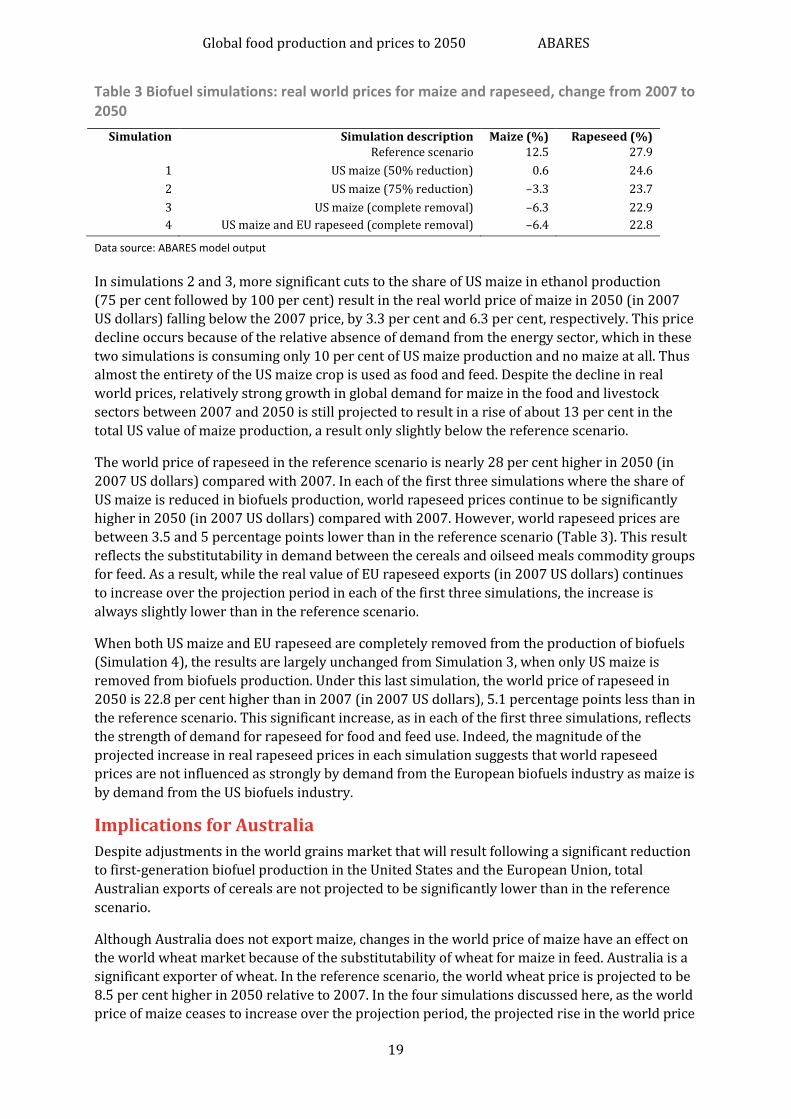
Table 3 Biofuel simulations: real world prices for maize and rapeseed, change from 2007 to 2050
Simulation Simulation description Maize (%) Rapeseed (%) Reference scenario 12.5 27.9
1 US maize (50% reduction) 0.6 24.6
2 US maize (75% reduction) –3.3 23.7
3 US maize (complete removal) –6.3 22.9
4 US maize and EU rapeseed (complete removal) –6.4 22.8
Data source: ABARES model output
In simulations 2 and 3, more significant cuts to the share of US maize in ethanol production
(75 per cent followed by 100 per cent) result in the real world price of maize in 2050 (in 2007
US dollars) falling below the 2007 price, by 3.3 per cent and 6.3 per cent, respectively. This price
decline occurs because of the relative absence of demand from the energy sector, which in these
two simulations is consuming only 10 per cent of US maize production and no maize at all. Thus
almost the entirety of the US maize crop is used as food and feed. Despite the decline in real
world prices, relatively strong growth in global demand for maize in the food and livestock
sectors between 2007 and 2050 is still projected to result in a rise of about 13 per cent in the
total US value of maize production, a result only slightly below the reference scenario.
The world price of rapeseed in the reference scenario is nearly 28 per cent higher in 2050 (in
2007 US dollars) compared with 2007. In each of the first three simulations where the share of
US maize is reduced in biofuels production, world rapeseed prices continue to be significantly
higher in 2050 (in 2007 US dollars) compared with 2007. However, world rapeseed prices are
between 3.5 and 5 percentage points lower than in the reference scenario (Table 3). This result
reflects the substitutability in demand between the cereals and oilseed meals commodity groups
for feed. As a result, while the real value of EU rapeseed exports (in 2007 US dollars) continues
to increase over the projection period in each of the first three simulations, the increase is
always slightly lower than in the reference scenario.
When both US maize and EU rapeseed are completely removed from the production of biofuels
(Simulation 4), the results are largely unchanged from Simulation 3, when only US maize is
removed from biofuels production. Under this last simulation, the world price of rapeseed in
2050 is 22.8 per cent higher than in 2007 (in 2007 US dollars), 5.1 percentage points less than in
the reference scenario. This significant increase, as in each of the first three simulations, reflects
the strength of demand for rapeseed for food and feed use. Indeed, the magnitude of the
projected increase in real rapeseed prices in each simulation suggests that world rapeseed
prices are not influenced as strongly by demand from the European biofuels industry as maize is
by demand from the US biofuels industry.
Implications for Australia
Despite adjustments in the world grains market that will result following a significant reduction
to first-generation biofuel production in the United States and the European Union, total
Australian exports of cereals are not projected to be significantly lower than in the reference
scenario.
Although Australia does not export maize, changes in the world price of maize have an effect on
the world wheat market because of the substitutability of wheat for maize in feed. Australia is a
significant exporter of wheat. In the reference scenario, the world wheat price is projected to be
8.5 per cent higher in 2050 relative to 2007. In the four simulations discussed here, as the world
price of maize ceases to increase over the projection period, the projected rise in the world price

Global food production and prices to 2050 ABARES
20
of wheat is lower than in the reference scenario. When both US maize and EU rapeseed are
completely removed from the production of biofuels (Simulation 4), the world price of wheat is
6.6 per cent higher in 2050 relative to 2007, nearly 2 percentage points lower than in the
reference scenario. This occurs as a result of weakening demand for feed wheat in lieu of maize,
which has an impact on Australian wheat exports. Although the value of Australian wheat
exports (in 2007 US dollars) in each of the scenarios is projected to be higher in 2050 relative to
2007 (between 62 per cent and 63 per cent higher), this increase is still marginally lower than in
the reference scenario (64.6 per cent).
For rapeseed (canola), Australia competes directly with the European Union on the world
market for both rapeseed oil and meal. The projected changes in real world rapeseed prices in
2050 relative to 2007 (in 2007 US dollars) in each of the four biofuels simulations is projected to
have an effect on the real value of Australian rapeseed production and exports, although the
response will be lower than in the reference scenario. In the reference scenario, the increase in
the value of Australian rapeseed exports is 105 per cent in 2050 relative to 2007. Over the four
simulations, increases in Australian rapeseed exports are between 96 per cent and 99 per cent.
Global food production and prices to 2050 ABARES
21
3 Conclusions Under the assumptions established in the reference scenario model simulation, world agrifood
prices are projected to be 11.5 per cent higher in 2050 compared with 2007 (in 2007 US
dollars). This increase is driven by stronger global demand stemming from increasing incomes
and population and resource constraints that are likely to affect productivity increases. The
price increase is projected to be lower than in the reference scenario when agrifood trade is
liberalised with additional increases in productivity growth rates. When the production of first-
generation biofuels in the United States and European Union is reduced, the simulation results
indicate a significant impact on world cereal prices.
In the reference scenario, the real value of world agrifood production (in 2007 US dollars) is
projected to be 75 per cent higher in 2050 compared with 2007. However, when trade is more
liberalised, the rise in the real value of world agrifood production by 2050 is projected to be
higher than the reference scenario, at 86 per cent. One model limitation for this study is that no
adjustments to productivity growth between periods are assumed—adjustments that might
come from innovation. If these adjustments could be incorporated in the model, as was done in
the trade liberalisation scenario, the production response to higher prices in the reference
scenario might be different. The results for each of the scenarios presented in this report are
merely indicative of one potential set of responses to a given set of assumptions.
These scenarios highlight the effect policy can have on agricultural prices, and the market
response to the removal of distortions. The policy environment will be instrumental in meeting
the demand for agrifood to 2050 in a sustainable manner, particularly given resource
constraints. To ensure food goes where it is needed, the policy agenda must include the
limitation and removal of trade restrictions, as well as the utilisation of resources by the most
efficient regions and sectors.
The simulations discussed in this report emphasise the significance of improvements in
productivity to meet higher food consumption and reduce price pressures. As was seen in the
sensitivity analysis, a small improvement in total factor productivity above a reference scenario
can lead to significantly lower global price rises over the longer term. In order to attain higher
productivity growth greater investment in research, development and extension and
infrastructure development is required.
Australia is well located to take advantage of the opportunities that higher food consumption
will provide but there will be a need for a change to agricultural production in Australia to fully
capture these opportunities. This will only be accomplished with a reversal of the recent slowing
rate of growth in productivity and more targeting of consumer needs in the growth areas of the
world—particularly Asia.
At the industry level, this will require targeting of our products to more diversified markets and
targeting different qualities of our products to market segments where there is greatest
potential for value adding. Such qualities could include, for example, safe, low pest,
environmentally sound, animal friendly products; products with a low carbon footprint or any
combination thereof. The relationship between prices and production is dynamic. Global
agrifood production adjusts to the incentives and opportunities inherent in market price
movements. Higher prices can lead to higher productivity by improving incentives for
investment in research and development, through innovation and through adaptation of existing
overseas technologies applied to an Australian environment. In so doing, producers will be able
to better cope with climatic challenges and land and water constraints.

Global food production and prices to 2050 ABARES
22
The government can also assist through a strong commitment to furthering global trade
liberalisation and increasing access to a diverse range of overseas markets. The government has
a role in providing information to support sound decision-making and to correct information
imbalances in the marketplace. It also has a role in education and training to ensure skills are
available. Governments will need to continue to provide a sound economic environment, with
appropriate fiscal policy settings that encourage economic and productivity growth—goals
achievable only if regulation is limited to those areas where market failures exist and where the
benefits of regulation clearly outweigh its costs.
Global food production and prices to 2050 ABARES
23
Appendix A: ABARES agrifood model For this analysis, ABARES used the agrifood model developed for Food demand to 2050:
Opportunities for Australian agriculture (Linehan et al. 2012a & 2012b). The model is an
economic simulation model of global agricultural supply, demand and trade. As in earlier
analysis, the model was used to prepare annual projections for 2007 to 2050. Annual regional
demand and supply curves are specified for each agrifood commodity. World prices, expressed
in real terms, balance global demand and supply for each commodity.
In the model, agrifood is defined as agricultural and fishery output that is used for food. This
includes food for human consumption, animal feed and food crops used as feedstock for other
purposes, such as biofuels. It does not include non-food agricultural outputs such as cotton or
wool.
Consumer demand for each commodity changes over time in the agrifood model, given
assumptions relating to real per person income and population. Commodities are linked through
substitution responses to relative price changes, which are themselves derived in the model. The
production of commodities increase with assumed rates of technical advancement. Crop
production is linked through competing land use. Livestock feed use competes with human
consumption and industrial feedstock use, and also with crop production for land for pasture.
The supply of land for agriculture, either for cropping or grazing, is price responsive, although
the availability of total arable land is limited. Low-value and high-value fish products are
incorporated in the model to account for possible protein options as well as to link with the feed
sector.
Key results from the model are expressed as real values to allow different commodities to be
aggregated. Real values are obtained by multiplying quantities in the projection years by world
prices in 2007, the model base year. For a single commodity, a given percentage change in real
value is equivalent to a pure volume change of the same percentage, assuming prices are
unchanged.
The two types of productivity improvements incorporated in the model are land productivity
and total factor productivity (TFP) improvements. Improvements in land productivity reflect a
reduction in the input of land per unit of output of cropping or livestock product. This is a partial
measure of productivity, where a single factor, land, experiences technological advancement (or
land productivity). TFP is a measure of total output relative to total inputs. In the modelling
framework, improvements in TFP are incorporated by applying changes in technological
improvement to every input, including land, feed conversion and an aggregate measure of other
inputs.
The model-based projections presented in the report are conditional on a set of assumptions,
most notably about the macro-economic environment and changes in agricultural technology
and productivity. Projections are also conditional on parameter values used to represent the
sensitivities of demand and supply curves to economic forces. Changes to these assumptions and
parameters result in changes to the projections.
New information and data has been incorporated into the model for this study. In particular, the
productivity growth assumptions for this study were sourced from a model comparison
exercise, the Agricultural Modelling Intercomparison and Improvement Project (AgMIP),
undertaken by ABARES and other research institutions (Rosenzweig et al. 2012), and are treated
as exogenous to the model. The land productivity assumptions for crops were derived from the
Global food production and prices to 2050 ABARES
24
International Food Policy Research Institute’s IMPACT model (Rosegrant et al. 2012). Land
productivity estimates for the livestock sectors were derived from the ABARES Global Trade and
Environment model (GTEM), and are capped at 3 per cent in any region. No technology catch-up
is reflected or imposed on these numbers.
With the exception of Australia, global maximum land availability figures for cropping and
pasture land are sourced from Alexandratos and Bruinsma (2012), and are mapped to the
regions in the agrifood model. For Australia, ABARES assumptions are used.
In the ABARES agrifood model a capture fishery is constrained to produce within, or on, an
exogenously set quota, depending on the most profitable option. Given the biophysical
constraints to expansion of global capture fisheries, quotas have been set equal to the base year
level of production for both high-value and low-value capture fisheries. One limitation of the
fisheries component of the model is the use of the fish meal and oil commodity group as the only
feed input in aquaculture production. In reality, aquafeed also includes animal protein meals and
fats as well as plant nutrients, such as cereals, oilseed meals and oilseed oils.
Information on the share of US maize, EU rapeseed, and Chinese wheat and maize used for
biofuels production was sourced from the International Grains Council (IGC 2012). The share of
Brazilian sugar used in ethanol production was sourced from OECD/FAO (2012).
A more detailed description of the model can be found in Linehan and colleagues (2012a and
2012b).
The model-based projections presented in this report are conditional on a set of assumptions.
Assumptions about the annual average growth rate in real incomes for each region in the model
are presented in Table A3.
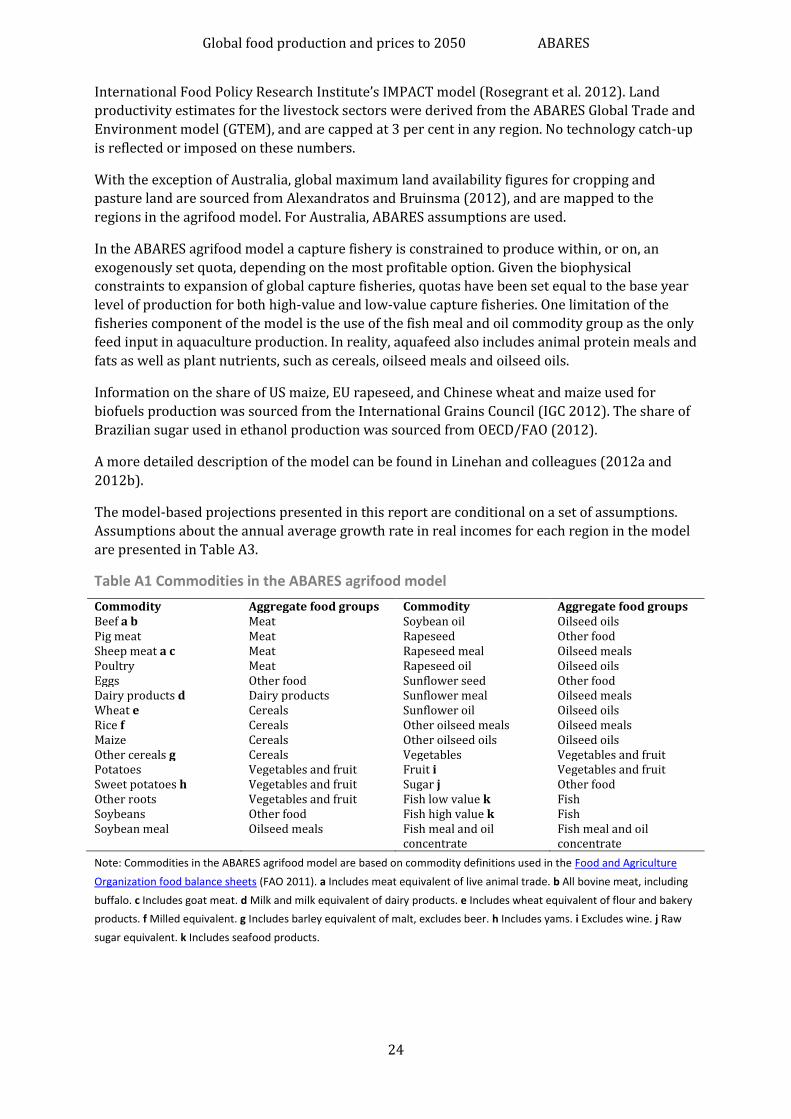
Table A1 Commodities in the ABARES agrifood model
Commodity Aggregate food groups Commodity Aggregate food groups Beef a b Meat Soybean oil Oilseed oils Pig meat Meat Rapeseed Other food Sheep meat a c Meat Rapeseed meal Oilseed meals Poultry Meat Rapeseed oil Oilseed oils Eggs Other food Sunflower seed Other food Dairy products d Dairy products Sunflower meal Oilseed meals Wheat e Cereals Sunflower oil Oilseed oils Rice f Cereals Other oilseed meals Oilseed meals Maize Cereals Other oilseed oils Oilseed oils Other cereals g Cereals Vegetables Vegetables and fruit Potatoes Vegetables and fruit Fruit i Vegetables and fruit Sweet potatoes h Vegetables and fruit Sugar j Other food Other roots Vegetables and fruit Fish low value k Fish Soybeans Other food Fish high value k Fish Soybean meal Oilseed meals Fish meal and oil
concentrate Fish meal and oil concentrate
Note: Commodities in the ABARES agrifood model are based on commodity definitions used in the Food and Agriculture
Organization food balance sheets (FAO 2011). a Includes meat equivalent of live animal trade. b All bovine meat, including
buffalo. c Includes goat meat. d Milk and milk equivalent of dairy products. e Includes wheat equivalent of flour and bakery
products. f Milled equivalent. g Includes barley equivalent of malt, excludes beer. h Includes yams. i Excludes wine. j Raw
sugar equivalent. k Includes seafood products.

Global food production and prices to 2050 ABARES
25
Table A2 Regions in the ABARES agrifood model
United States Central Asia b Thailand Rest of Oceania j Canada India Vietnam Egypt Mexico Pakistan Rest of South East Asia d Rest of North Africa Brazil Bangladesh West Asia e Nigeria Argentina Sri Lanka Turkey Rest of Middle and
Western Africa Rest of America Rest of South Asia c European Union 15 f Republic of South Africa Japan Indonesia Eastern Europe g Rest of Southern and
Eastern Africa Republic of Korea Malaysia Southern Europe h China Myanmar Rest of Europe i Rest of East Asia a Philippines Australia
Note: Regions used in the ABARES agrifood model are based on United Nations geographical regions (United Nations 2011).
a China (Hong Kong) Special Administrative Region, China (Macao) Special Administrative Region, Democratic People’s
Republic of Korea and Mongolia. b Kazakhstan, Kyrgyzstan, Tajikistan, Turkmenistan and Uzbekistan. c Afghanistan, Bhutan,
Islamic Republic of Iran, Maldives and Nepal. d Brunei Darussalam, Cambodia, Lao People’s Democratic Republic, Singapore
and Timor-Leste. e Armenia, Azerbaijan, Bahrain, Cyprus, Georgia, Iraq, Israel, Jordan, Kuwait, Lebanon, Occupied
Palestinian Territory, Oman, Saudi Arabia, Syrian Arab Republic and United Arab Emirates. f Austria, Belgium, Denmark,
Finland, France, Germany, Greece, Ireland, Italy, Luxembourg, the Netherlands, Portugal, Spain, Sweden and the United
Kingdom. g Belarus, Bulgaria, Czech Republic, Hungary, Poland, Republic of Moldova, Romania, Russian Federation, Slovakia
and Ukraine. h Albania, Andorra, Bosnia and Herzegovina, Croatia, Gibraltar, Holy See, Malta, Montenegro, San Marino,
Serbia, Slovenia, and the Former Yugoslav Republic of Macedonia. i Åland Islands, Channel Islands, Estonia, Faeroe Islands,
Guernsey, Iceland, Isle of Man, Jersey, Latvia, Lithuania, Norway, Sark, Svalbard and Jan Mayen islands, Lichtenstein,
Monaco and Switzerland. j Predominantly New Zealand.
Table A3 Average annual real income growth, 2007 to 2050
Country or region Annual real income growth (%)
Country or region Annual real income growth (%)
United States 2.3 Philippines 3.8 Canada 1.9 Thailand 2.7 Mexico 2.4 Vietnam 4.3 Brazil 3.0 Rest of South East Asia 2.7 Argentina 3.3 West Asia 3.6 Rest of America 3.0 Turkey 2.6 Japan 1.1 European Union 15 1.4 Republic of Korea 2.2 Eastern Europe 2.4 China 5.5 Southern Europe 1.6 Rest of East Asia 3.0 Rest of Europe 1.7 Central Asia 3.9 Australia 2.6 India 5.4 Rest of Europe 2.5 Pakistan 3.5 Egypt 3.2 Bangladesh 4.3 Rest of North Africa 3.2 Sri Lanka 4.3 Nigeria 5.5 Rest of South Asia 4.9 Rest of Middle and
Western Africa 4.6
Indonesia 4.2 Republic of South Africa 3.0 Malaysia 3.6 Rest of Southern and
Eastern Africa 5.3
Myanmar 4.3
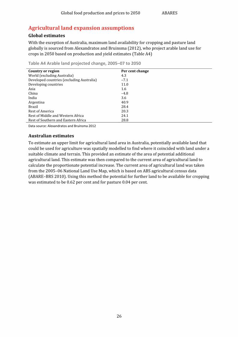
Global food production and prices to 2050 ABARES
26
Agricultural land expansion assumptions
Global estimates
With the exception of Australia, maximum land availability for cropping and pasture land
globally is sourced from Alexandratos and Bruinsma (2012), who project arable land use for
crops in 2050 based on production and yield estimates (Table A4)
Table A4 Arable land projected change, 2005–07 to 2050
Country or region Per cent change World (excluding Australia) 4.3 Developed countries (excluding Australia) –7.1 Developing countries 11.0 Asia 1.6 China –4.8 India 3.6 Argentina 40.9 Brazil 28.4 Rest of America 20.3 Rest of Middle and Western Africa 24.1 Rest of Southern and Eastern Africa 28.8
Data source: Alexandratos and Bruinsma 2012
Australian estimates
To estimate an upper limit for agricultural land area in Australia, potentially available land that
could be used for agriculture was spatially modelled to find where it coincided with land under a
suitable climate and terrain. This provided an estimate of the area of potential additional
agricultural land. This estimate was then compared to the current area of agricultural land to
calculate the proportionate potential increase. The current area of agricultural land was taken
from the 2005–06 National Land Use Map, which is based on ABS agricultural census data
(ABARE–BRS 2010). Using this method the potential for further land to be available for cropping
was estimated to be 0.62 per cent and for pasture 0.04 per cent.
Global food production and prices to 2050 ABARES
27
Appendix B: Factors affecting future food production
Land availability
While studies suggest plenty of arable land is available globally, much of this land is located in
Latin America and sub-Saharan Africa, and may be inaccessible, lack agricultural infrastructure
or be diseased. Land constraints at the country or regional level can be significant, with a
number of countries having reached, or about to reach the limits of their available land for
agriculture. At the same time, competition exists for this land for urbanisation, industrial,
environmental and recreational uses (OECD/FAO 2012).
The continuing decline of agricultural land availability is often cited as an indicator of difficulties
in meeting future food demand. However, Alexandratos and Bruinsma (2012) suggest that
changes in land use will be the result of countervailing forces—population, demand growth and
increasing crop yields—and the outcome will differ between countries.
Alexandratos and Bruinsma (2012) project that between 2005–07 and 2050 the area of arable
land suitable for cropping use will increase by 70 million hectares (4.3 per cent). Developing
countries are projected to increase arable land by almost 110 million hectares, while the arable
land area for developed countries is projected to fall by about 40 million hectares. The bulk of
the projected expansion is expected to take place in sub-Saharan Africa (51 million hectares)
and Latin America (49 million hectares), with almost no land expansion in South Asia, and a
constant area in the Middle East, North Africa and East Asia.
Productivity
A number of factors are expected to affect agricultural productivity include land degradation,
limitations in water availability and climate change.
Land degradation
Land degradation is the long-term decline in ecosystem function (Bai et al. 2008). It is an
ongoing global issue that affects soils, biomass, water, biodiversity and socio-economic services
derived from ecosystems (Nachtergaele et al. 2011). Land degradation processes include
vegetation degradation, loss in quantity and quality of water resources, and soil degradation,
such as erosion, salinisation, loss of nutrients, acidification, and physical and biological
degradation (FAO 1999). The OECD/FAO (2012) estimate that approximately 25 per cent of the
world’s agricultural land area is highly degraded.
Soil degradation in drylands is a significant contributor to the reduction of soil fertility and, in
turn, agricultural productivity. Based on available data in 2010, the United Nations Convention
to Combat Desertification found that 44 per cent of global food production takes place in the
world’s drylands, and that 52 per cent of the land used for agriculture is moderately or severely
affected by land degradation (UNCCD 2010).
Water quality and availability
Water availability is a constraint on agriculture and agricultural expansion, especially in the
dryland regions. Competing uses, such as urbanisation and industrial activity, can and do
exacerbate water shortages. Irrigation has been widely adopted as one way to ensure constancy
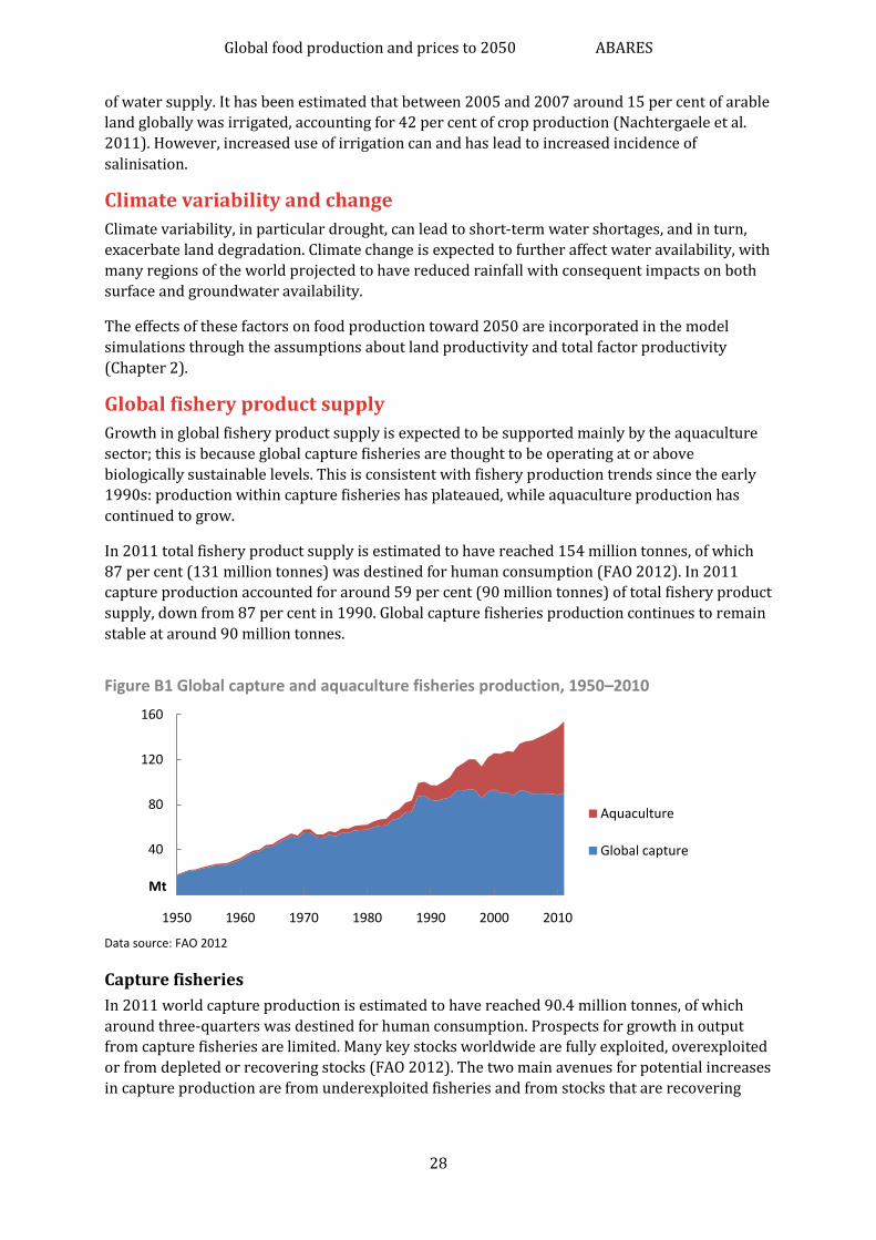
Global food production and prices to 2050 ABARES
28
of water supply. It has been estimated that between 2005 and 2007 around 15 per cent of arable
land globally was irrigated, accounting for 42 per cent of crop production (Nachtergaele et al.
2011). However, increased use of irrigation can and has lead to increased incidence of
salinisation.
Climate variability and change
Climate variability, in particular drought, can lead to short-term water shortages, and in turn,
exacerbate land degradation. Climate change is expected to further affect water availability, with
many regions of the world projected to have reduced rainfall with consequent impacts on both
surface and groundwater availability.
The effects of these factors on food production toward 2050 are incorporated in the model
simulations through the assumptions about land productivity and total factor productivity
(Chapter 2).
Global fishery product supply
Growth in global fishery product supply is expected to be supported mainly by the aquaculture
sector; this is because global capture fisheries are thought to be operating at or above
biologically sustainable levels. This is consistent with fishery production trends since the early
1990s: production within capture fisheries has plateaued, while aquaculture production has
continued to grow.
In 2011 total fishery product supply is estimated to have reached 154 million tonnes, of which
87 per cent (131 million tonnes) was destined for human consumption (FAO 2012). In 2011
capture production accounted for around 59 per cent (90 million tonnes) of total fishery product
supply, down from 87 per cent in 1990. Global capture fisheries production continues to remain
stable at around 90 million tonnes.
Figure B1 Global capture and aquaculture fisheries production, 1950–2010
Data source: FAO 2012
Capture fisheries
In 2011 world capture production is estimated to have reached 90.4 million tonnes, of which
around three-quarters was destined for human consumption. Prospects for growth in output
from capture fisheries are limited. Many key stocks worldwide are fully exploited, overexploited
or from depleted or recovering stocks (FAO 2012). The two main avenues for potential increases
in capture production are from underexploited fisheries and from stocks that are recovering
40
80
120
160
1950 1960 1970 1980 1990 2000 2010
Mt
Aquaculture
Global capture
Global food production and prices to 2050 ABARES
29
under a sound management strategy. Little production growth from fully exploited,
overexploited or depleted fisheries is expected up to 2050.
Underexploited fisheries represent a relatively small proportion of fishery resources (FAO
2005). They are underexploited primarily because, with current technology, it is not
economically viable to harvest at higher levels. However, under appropriate management, and
with more efficient fishing technology and/or the development of new seafood markets, these
fisheries could increase production and improve their economic viability.
Recovering fisheries could increase production up to 2050, provided stocks are rebuilt to a point
where higher sustainable harvests are possible. However, increased production in these
fisheries relies on sound management strategies to ensure recovery and environmental factors
conducive to stock recovery. The ability of many management regimes to facilitate stock
recovery remains unproven.
Aquaculture
Most of the growth in global seafood production up to 2050 is expected to be sourced from
aquaculture. Over the past three decades, global seafood production of aquaculture grew at an
average annual rate of 8.8 per cent. In 2010 global edible aquaculture production reached a peak
of 60 million tonnes.
To meet future demand for food from aquaculture, production will largely depend on the
availability of quality feeds. Growth of the aquaculture sector may also be limited by natural
factors. For example, growth in the production of the non-fed sector, that is species that do not
rely on fish feed, but only natural food sources, may be limited by the availability of suitable
sites. Similarly, growth in the fed sector (species that rely on fish feed) may be limited by the
availability of fish meal and fish oil from capture species, which are major ingredients in
aquaculture fish feed. Aquaculture production is also vulnerable to the adverse effects of disease
and environmental conditions.
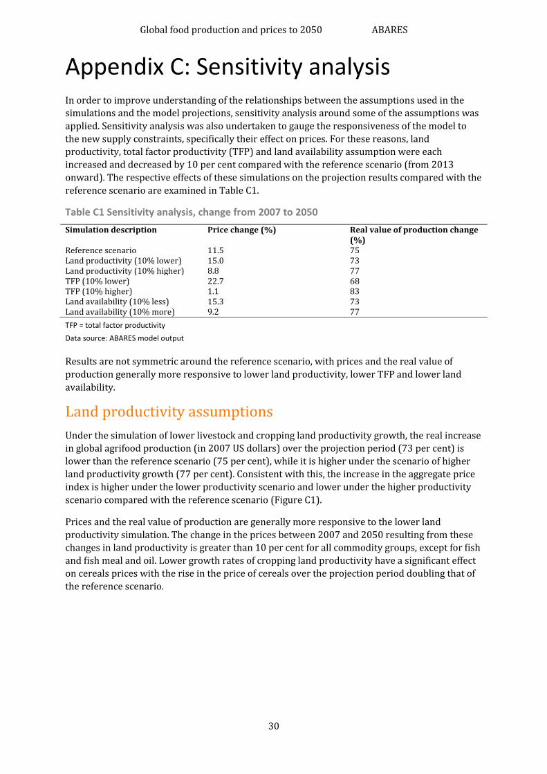
Global food production and prices to 2050 ABARES
30
Appendix C: Sensitivity analysis In order to improve understanding of the relationships between the assumptions used in the
simulations and the model projections, sensitivity analysis around some of the assumptions was
applied. Sensitivity analysis was also undertaken to gauge the responsiveness of the model to
the new supply constraints, specifically their effect on prices. For these reasons, land
productivity, total factor productivity (TFP) and land availability assumption were each
increased and decreased by 10 per cent compared with the reference scenario (from 2013
onward). The respective effects of these simulations on the projection results compared with the
reference scenario are examined in Table C1.
Table C1 Sensitivity analysis, change from 2007 to 2050
Simulation description Price change (%) Real value of production change (%)
Reference scenario 11.5 75 Land productivity (10% lower) 15.0 73 Land productivity (10% higher) 8.8 77 TFP (10% lower) 22.7 68 TFP (10% higher) 1.1 83 Land availability (10% less) 15.3 73 Land availability (10% more) 9.2 77
TFP = total factor productivity
Data source: ABARES model output
Results are not symmetric around the reference scenario, with prices and the real value of
production generally more responsive to lower land productivity, lower TFP and lower land
availability.
Land productivity assumptions
Under the simulation of lower livestock and cropping land productivity growth, the real increase
in global agrifood production (in 2007 US dollars) over the projection period (73 per cent) is
lower than the reference scenario (75 per cent), while it is higher under the scenario of higher
land productivity growth (77 per cent). Consistent with this, the increase in the aggregate price
index is higher under the lower productivity scenario and lower under the higher productivity
scenario compared with the reference scenario (Figure C1).
Prices and the real value of production are generally more responsive to the lower land
productivity simulation. The change in the prices between 2007 and 2050 resulting from these
changes in land productivity is greater than 10 per cent for all commodity groups, except for fish
and fish meal and oil. Lower growth rates of cropping land productivity have a significant effect
on cereals prices with the rise in the price of cereals over the projection period doubling that of
the reference scenario.

Global food production and prices to 2050 ABARES
31
Figure C1 Land productivity sensitivity—world real food, change from 2007 to 2050
Data source: ABARES model output
The real value of cereals production is sensitive to the change in land productivity (Figure C2). In
the lower land productivity simulation, the real value of cereals production (in 2007 US dollars)
in 2050 is 34.8 per cent higher than 2007, while under the reference scenario it is 42.2 per cent
higher, and under the higher land productivity simulation it is 48.5 per cent higher. As a result of
lower land productivity for livestock and higher feed input costs, the real value of meat
production in 2050 is projected to be 106 per cent higher than in 2007 in the lower land
productivity simulation, lower than the rise in the reference scenario (110 per cent) and in the
higher land productivity simulation (115 per cent).
Figure C2 Land productivity sensitivity—world real value of production under high and low land productivity growth, change from 2007 to 2050
Data source: ABARES model output
-20 0 20 40 60 80
Oilseed meal
Dairy products
Vegetables and fruit
Other food
Cereals
Oilseed oils
Meat
Fish
Fish meal and oil
Total
%
Reference scenarioHigher land productivityLower land productivity
50 100 150
Fish meal and oil
Oilseed meal
Oilseed oils
Cereals
Other food
Fish
Vegetables and fruit
Dairy products
Meat
Total
%
Reference scenarioHigher land productivityLower land productivity
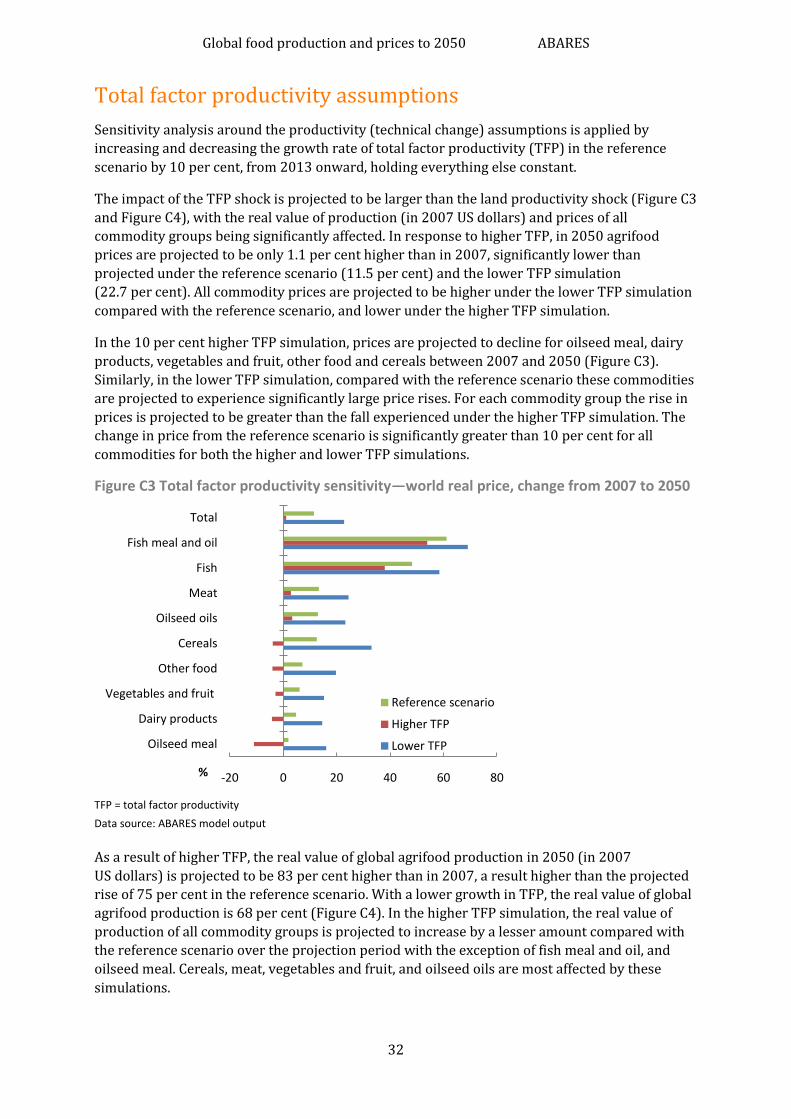
Global food production and prices to 2050 ABARES
32
Total factor productivity assumptions
Sensitivity analysis around the productivity (technical change) assumptions is applied by
increasing and decreasing the growth rate of total factor productivity (TFP) in the reference
scenario by 10 per cent, from 2013 onward, holding everything else constant.
The impact of the TFP shock is projected to be larger than the land productivity shock (Figure C3
and Figure C4), with the real value of production (in 2007 US dollars) and prices of all
commodity groups being significantly affected. In response to higher TFP, in 2050 agrifood
prices are projected to be only 1.1 per cent higher than in 2007, significantly lower than
projected under the reference scenario (11.5 per cent) and the lower TFP simulation
(22.7 per cent). All commodity prices are projected to be higher under the lower TFP simulation
compared with the reference scenario, and lower under the higher TFP simulation.
In the 10 per cent higher TFP simulation, prices are projected to decline for oilseed meal, dairy
products, vegetables and fruit, other food and cereals between 2007 and 2050 (Figure C3).
Similarly, in the lower TFP simulation, compared with the reference scenario these commodities
are projected to experience significantly large price rises. For each commodity group the rise in
prices is projected to be greater than the fall experienced under the higher TFP simulation. The
change in price from the reference scenario is significantly greater than 10 per cent for all
commodities for both the higher and lower TFP simulations.
Figure C3 Total factor productivity sensitivity—world real price, change from 2007 to 2050
TFP = total factor productivity
Data source: ABARES model output
As a result of higher TFP, the real value of global agrifood production in 2050 (in 2007
US dollars) is projected to be 83 per cent higher than in 2007, a result higher than the projected
rise of 75 per cent in the reference scenario. With a lower growth in TFP, the real value of global
agrifood production is 68 per cent (Figure C4). In the higher TFP simulation, the real value of
production of all commodity groups is projected to increase by a lesser amount compared with
the reference scenario over the projection period with the exception of fish meal and oil, and
oilseed meal. Cereals, meat, vegetables and fruit, and oilseed oils are most affected by these
simulations.
-20 0 20 40 60 80
Oilseed meal
Dairy products
Vegetables and fruit
Other food
Cereals
Oilseed oils
Meat
Fish
Fish meal and oil
Total
%
Reference scenario
Higher TFP
Lower TFP
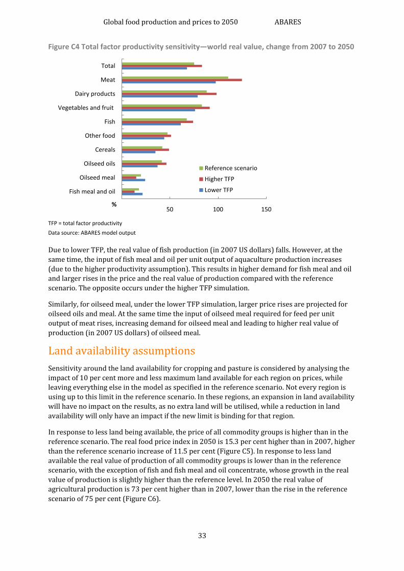
Global food production and prices to 2050 ABARES
33
Figure C4 Total factor productivity sensitivity—world real value, change from 2007 to 2050
TFP = total factor productivity
Data source: ABARES model output
Due to lower TFP, the real value of fish production (in 2007 US dollars) falls. However, at the
same time, the input of fish meal and oil per unit output of aquaculture production increases
(due to the higher productivity assumption). This results in higher demand for fish meal and oil
and larger rises in the price and the real value of production compared with the reference
scenario. The opposite occurs under the higher TFP simulation.
Similarly, for oilseed meal, under the lower TFP simulation, larger price rises are projected for
oilseed oils and meal. At the same time the input of oilseed meal required for feed per unit
output of meat rises, increasing demand for oilseed meal and leading to higher real value of
production (in 2007 US dollars) of oilseed meal.
Land availability assumptions
Sensitivity around the land availability for cropping and pasture is considered by analysing the
impact of 10 per cent more and less maximum land available for each region on prices, while
leaving everything else in the model as specified in the reference scenario. Not every region is
using up to this limit in the reference scenario. In these regions, an expansion in land availability
will have no impact on the results, as no extra land will be utilised, while a reduction in land
availability will only have an impact if the new limit is binding for that region.
In response to less land being available, the price of all commodity groups is higher than in the
reference scenario. The real food price index in 2050 is 15.3 per cent higher than in 2007, higher
than the reference scenario increase of 11.5 per cent (Figure C5). In response to less land
available the real value of production of all commodity groups is lower than in the reference
scenario, with the exception of fish and fish meal and oil concentrate, whose growth in the real
value of production is slightly higher than the reference level. In 2050 the real value of
agricultural production is 73 per cent higher than in 2007, lower than the rise in the reference
scenario of 75 per cent (Figure C6).
50 100 150
Fish meal and oil
Oilseed meal
Oilseed oils
Cereals
Other food
Fish
Vegetables and fruit
Dairy products
Meat
Total
%
Reference scenario
Higher TFP
Lower TFP
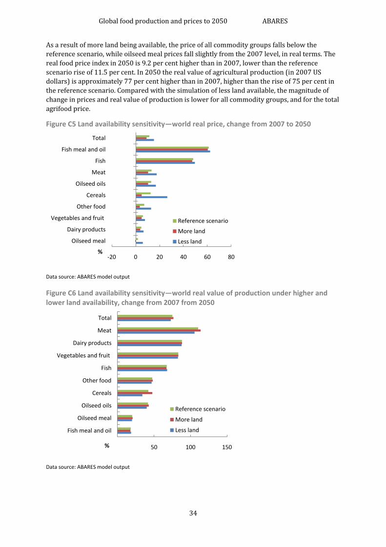
Global food production and prices to 2050 ABARES
34
As a result of more land being available, the price of all commodity groups falls below the
reference scenario, while oilseed meal prices fall slightly from the 2007 level, in real terms. The
real food price index in 2050 is 9.2 per cent higher than in 2007, lower than the reference
scenario rise of 11.5 per cent. In 2050 the real value of agricultural production (in 2007 US
dollars) is approximately 77 per cent higher than in 2007, higher than the rise of 75 per cent in
the reference scenario. Compared with the simulation of less land available, the magnitude of
change in prices and real value of production is lower for all commodity groups, and for the total
agrifood price.
Figure C5 Land availability sensitivity—world real price, change from 2007 to 2050
Data source: ABARES model output
Figure C6 Land availability sensitivity—world real value of production under higher and lower land availability, change from 2007 from 2050
Data source: ABARES model output
-20 0 20 40 60 80
Oilseed meal
Dairy products
Vegetables and fruit
Other food
Cereals
Oilseed oils
Meat
Fish
Fish meal and oil
Total
%
Reference scenario
More land
Less land
50 100 150
Fish meal and oil
Oilseed meal
Oilseed oils
Cereals
Other food
Fish
Vegetables and fruit
Dairy products
Meat
Total
%
Reference scenario
More land
Less land

Global food production and prices to 2050 ABARES
35
References Alexandratos, N & Bruinsma, J 2012, World agriculture toward 2030/2050: the 2012 revision, ESA
Working paper no. 12-03, Food and Agriculture Organization of the United Nations,
Rome, available at fao.org/economic/esa/esag/en.
ABARE–BRS 2010, Land Use of Australia Version 4, 2005–06, Department of Agriculture,
Fisheries and Forestry, ABARE–BRS, September.
ABARES 2007, Global Trade and Environment Model (GTEM), Australian Bureau of Agricultural
and Resource Economics and Sciences, Canberra, available at daff.gov.au/abares/publications.
Bai, ZG, Dent, DL, Olsson, L & Schaepman, ME 2008, Global assessment of land degradation and
improvement, 1. Identification by remote sensing, Report 2008/01, ISRIC World Soil Information,
Wageningen, Netherlands.
Chapman, S, Dreccer, F, Palta-Paz, J, Bourgault, M, Zheng, B, Wockner, K, Liu, W, Kearns, R, Dias
de Oliveira, E, Hammer, G, Chenu, K, Jordan, D, Singh, V, thi Chuc, N, van Oosterom, E, McLean, G
& Banks, P 2012, A national research program for climate ready cereals, Final Report June 2012,
Climate Change Research Program, Department of Agriculture Fisheries and Forestry, Canberra.
Lin, E, Xiong, W, Ju, Hui, Xu, Y, Li, Y, Bai, L & Xie, L 2005, ‘Climate change impacts on crop yield
and quality with CO2 fertilization in China’, Philosophical Transactions of the Royal Society, Series
B 29, vol. 360, no. 1463 pp. 2149–54.
EPA 2013, EPA 2013, ‘Regulation of Fuels and Fuel Additives: 2013 Renewable Fuel Standards’,
40 CFR Part 80, [EPA-HQ-OAR-2012-0546; FRL-9678-8], RIN 2060-AR43, United States
Environmental Protection Agency, Washington DC, available at
epa.gov/otaq/fuels/renewablefuels/documents/rfs-2013-standards-nrpm.pdf.
FAO 2013, ‘FAO Food Price Index’, released 10/01/2013, Food and Agriculture Organization of
the United Nations, Rome, available at fao.org/worldfoodsituation/wfs-
home/foodpricesindex/en/, accessed 18 January 2013.
FAO 2012, The state of world fisheries and aquaculture 2012, Food and Agriculture Organization
of the United Nations, Rome.
FAO 2011, ‘FAOSTAT’ [food balance sheets], Food and Agriculture Organization of the United
Nations, Rome, available at faostat.fao.org/site/655/default.aspx.
FAO 2005, ‘Review of the state of world marine fishery resources’, FAO fisheries technical paper,
no. 457, Food and Agriculture Organization of the United Nations, Rome, available at
fao.org/fi/oldsite/eims_search/1_dett.asp?lang=en&pub_id=172962.
FAO 1999 Poverty alleviation and food security in Asia: land resources, RAP Publication 1999/2,
Food and Agriculture Organization of the United Nations, Rome.
Global Issues In Context 2013, ‘Biofuel impact on food prices and world hunger’, Global Issues in
Context Online Collection, Gale, Detroit, 19 February, available at
find.galegroup.com/gic/docRetrieve.do?searchPageType=BasicSearchForm&inPS=true&prodId
=GIC&userGroupName=itsbtrial&docId=CP3208520015 (subscription only).
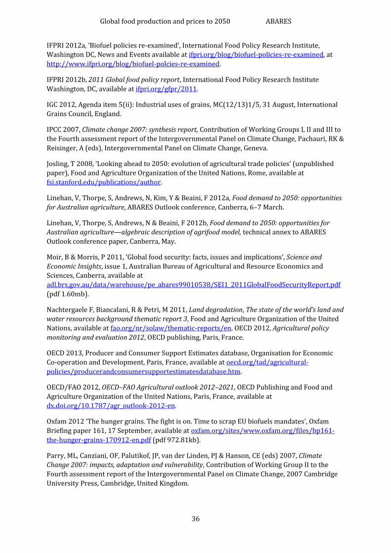
Global food production and prices to 2050 ABARES
36
IFPRI 2012a, ‘Biofuel policies re-examined’, International Food Policy Research Institute,
Washington DC, News and Events available at ifpri.org/blog/biofuel-policies-re-examined, at
http://www.ifpri.org/blog/biofuel-polcies-re-examined.
IFPRI 2012b, 2011 Global food policy report, International Food Policy Research Institute
Washington, DC, available at ifpri.org/gfpr/2011.
IGC 2012, Agenda item 5(ii): Industrial uses of grains, MC(12/13)1/5, 31 August, International
Grains Council, England.
IPCC 2007, Climate change 2007: synthesis report, Contribution of Working Groups I, II and III to
the Fourth assessment report of the Intergovernmental Panel on Climate Change, Pachauri, RK &
Reisinger, A (eds), Intergovernmental Panel on Climate Change, Geneva.
Josling, T 2008, ‘Looking ahead to 2050: evolution of agricultural trade policies’ (unpublished
paper), Food and Agriculture Organization of the United Nations, Rome, available at
fsi.stanford.edu/publications/author.
Linehan, V, Thorpe, S, Andrews, N, Kim, Y & Beaini, F 2012a, Food demand to 2050: opportunities
for Australian agriculture, ABARES Outlook conference, Canberra, 6–7 March.
Linehan, V, Thorpe, S, Andrews, N & Beaini, F 2012b, Food demand to 2050: opportunities for
Australian agriculture—algebraic description of agrifood model, technical annex to ABARES
Outlook conference paper, Canberra, May.
Moir, B & Morris, P 2011, ‘Global food security: facts, issues and implications’, Science and
Economic Insights, issue 1, Australian Bureau of Agricultural and Resource Economics and
Sciences, Canberra, available at
adl.brs.gov.au/data/warehouse/pe_abares99010538/SEI1_2011GlobalFoodSecurityReport.pdf
(pdf 1.60mb).
Nachtergaele F, Biancalani, R & Petri, M 2011, Land degradation, The state of the world’s land and
water resources background thematic report 3, Food and Agriculture Organization of the United
Nations, available at fao.org/nr/solaw/thematic-reports/en. OECD 2012, Agricultural policy
monitoring and evaluation 2012, OECD publishing, Paris, France.
OECD 2013, Producer and Consumer Support Estimates database, Organisation for Economic
Co-operation and Development, Paris, France, available at oecd.org/tad/agricultural-
policies/producerandconsumersupportestimatesdatabase.htm.
OECD/FAO 2012, OECD–FAO Agricultural outlook 2012–2021, OECD Publishing and Food and
Agriculture Organization of the United Nations, Paris, France, available at
dx.doi.org/10.1787/agr_outlook-2012-en.
Oxfam 2012 ‘The hunger grains. The fight is on. Time to scrap EU biofuels mandates’, Oxfam
Briefing paper 161, 17 September, available at oxfam.org/sites/www.oxfam.org/files/bp161-
the-hunger-grains-170912-en.pdf (pdf 972.81kb).
Parry, ML, Canziani, OF, Palutikof, JP, van der Linden, PJ & Hanson, CE (eds) 2007, Climate
Change 2007: impacts, adaptation and vulnerability, Contribution of Working Group II to the
Fourth assessment report of the Intergovernmental Panel on Climate Change, 2007 Cambridge
University Press, Cambridge, United Kingdom.
Global food production and prices to 2050 ABARES
37
Peters, GP, Andrew, RM, Boden, T, Canadell, JG, Ciais, P, Le Quéré, C, Marland, G, Raupach, M &
Wilson, C 2012, ‘The challenge to keep global warming below 2 °C’, Nature Climate Change,
advance online publication, available at nature.com/natureclimatechange.
Rosegrant, MW & the IMPACT Development Team 2012, International Model for Policy Analysis
of Agricultural Commodities and Trade (IMPACT): model description, International Food Policy
Research Institute, Washington, DC, available at ifpri.org/publication/international-model-
policy-analysis-agricultural-commodities-and-trade-impact-1.
Rosenzweig, C, Jones, JW, Hatfield JL, Ruane, AC, Boote, KJ, Thorburn, P, Antle, JM, Nelson, GC,
Porter, C, Janssen, S, Asseng, S, Basso, B, Ewert, F, Wallach, D, Baigorria, G & Winter, JM 2012,
‘The Agricultural Model Intercomparison and Improvement Project (AgMIP): protocols and pilot
studies’, Agricultural and Forest Meteorology, in press, available at agmip.org/refbase/index.php.
Rutherford, TF 1995, ‘Extension of GAMS for complementarity problems arising in applied
economic analysis’, Journal of Economic Dynamics and Control, vol. 19, no. 8, pp. 1299–324.
Sarris, A 2009, ‘Evolving structure of world agricultural trade and requirements for new world
trade rules’, paper prepared for How to feed the World in 2050: high-level expert forum, 12–13
October 2009, Food and Agriculture Organization of the United Nations, Economic and Social
Development Department, Rome, available at
ftp.fao.org/docrep/fao/012/ak979e/ak979e00.pdf (pdf 386.26kb).
Tausz, M 2012, ‘Adaptation of a range of wheat types to elevated atmospheric CO2
concentration’, Final report, Climate Change Research Program, Department of Agriculture
Fisheries and Forestry, Canberra.
United Nations 2011, ‘Composition of macro geographical (continental) regions, geographical
sub-regions, and selected economic and other groupings’, United Nations, New York, available at
unstats.un.org/unsd/methods/m49/m49regin.htm.
UNCCD 2010, Drylands soil: sustaining life on earth, United Nations Convention to Combat
Desertification, Bonn, Germany, available at
unccd.int/Lists/SiteDocumentLibrary/Publications/DrylandsSoilUNCCDBrochureFinal.pdf (pdf
881kb).
USDA 2012, ‘China—Peoples Republic, Biofuels Annual’, Gain Report Number 12044, 9 July,
Foreign Agriculture Service, US Department of Agriculture, Washington DC.