Global environmental drivers of influenzaEthan R. Deylea, M. Cyrus Maherb,c, Ryan D. Hernandezd, Sanjay Basue, and George Sugiharaa,1

aScripps Institution of Oceanography, University of California, San Diego, La Jolla, CA 92093; bHuman Longevity Inc., Mountain View, CA 94041; cDepartment ofEpidemiology and Translational Science, University of California, San Francisco, CA 94158; dDepartment of Bioengineering and Therapeutic Sciences, Universityof California, San Francisco, CA 94158; and eStanford Prevention Research Center, Stanford University School of Medicine, Stanford, CA 94305

Edited by Alan Hastings, University of California, Davis, CA, and approved September 16, 2016 (received for review May 13, 2016)

In temperate countries, influenza outbreaks are well correlated toseasonal changes in temperature and absolute humidity. However,tropical countries have much weaker annual climate cycles, andoutbreaks show less seasonality and are more difficult to explainwith environmental correlations. Here, we use convergent crossmapping, a robust test for causality that does not require correla-tion, to test alternative hypotheses about the global environmentaldrivers of influenza outbreaks from country-level epidemic timeseries. By moving beyond correlation, we show that despite theapparent differences in outbreak patterns between temperateand tropical countries, absolute humidity and, to a lesser extent,temperature drive influenza outbreaks globally. We also find ahypothesized U-shaped relationship between absolute humidity andinfluenza that is predicted by theory and experiment, but hitherto hasnot been documented at the population level. The balance betweenpositive and negative effects of absolute humidity appears to bemediated by temperature, and the analysis reveals a key thresholdaround 75 °F. The results indicate a unified explanation for environ-mental drivers of influenza that applies globally.

epidemiology | empirical dynamic modeling | nonlinear dynamics |state-dependence | physical–biological coupling

Adiverse group of drivers and mechanisms has been put for-ward to explain the wintertime occurrence of seasonal in-

fluenza outbreaks. Laboratory experiments show that relativehumidity controls droplet size and aerosol transmission rates (1).Experiments with mammalian models showed that viral sheddingby hosts increases at low temperature (2). Strong laboratoryevidence has emerged that absolute humidity has a controllingeffect on airborne influenza transmission (3).Nevertheless, questions remain as to how these potential

causal agents are expressed at the population level as epidemiccontrol variables. At the population level, environmental factorscovary, multiple mechanisms can coact, and infection dynamicsare influenced by many other important processes (4), such ashuman crowding, rapid viral evolution, and international travelpatterns. Perhaps not surprisingly, statistical analyses of pop-ulation level data have produced contradictory results. Althoughcorrelations between influenza incidence and both temperatureand absolute humidity are easy to find in temperate countries (5)and individual US states (6), such associations are weak or al-together absent in data from tropical countries (5).Here we use new methods appropriate for disease dynamics to

identify the causal drivers of influenza acting at the populationlevel. Using time series data across countries and latitudes, wefind that absolute humidity drives influenza across latitudes, andthat this effect is modulated by temperature. At low tempera-tures, absolute humidity negatively affects influenza incidence(drier conditions improve survival of the influenza virus when itis cold), but at high temperatures, absolute humidity positivelyaffects influenza (wetter conditions improve survival of the in-fluenza virus when it is warm). This population-level findingsupports the conclusions of theoretical work on viral envelopestability (7) and sorts out disagreements in laboratory studies (8).Our analysis is divided into three parts. First, we show how

dynamic resonance can explain the success of linear statisticalmethods in detecting causal effects in temperate latitudes and how

mirage correlations are symptoms of their failure in the tropics.This motivates taking an empirical dynamic modeling (EDM)approach (9). Second, we use the EDM method of detecting cau-sality, convergent cross-mapping (CCM), to show how absolutehumidity and temperature combine to produce a unified expla-nation for influenza outbreaks that applies across latitudes. Fi-nally, we probe the mechanistic effects of each variable, showingthat absolute humidity has the most direct effect on influenza,and that this effect is modulated nonlinearly by temperature.

ResultsCorrelation and Seasonality. It is well known that correlative ap-proaches can fail to provide an accurate picture of cause andeffect in a dynamic system, and this is especially true in nonlinearsystems where interdependence between variables is complex.Such systems are known to produce mirage correlations thatappear, disappear, and even reverse sign over time (9). Persistentcorrelations tend to only occur in specific circumstances; mostnotably, when there is synchrony between driver and responsevariables (the effect of the driving variable is strong enough thatthe response becomes enslaved to the driver). This is key, be-cause basic host–pathogen dynamics are known to exhibit dy-namical resonance when strongly forced by periodic drivers (10).Dynamical resonance causes the intrinsic nonlinear epidemio-logical dynamics to become synchronized (phase-locked) to thesimple cyclic motion of the environmental driver. However,when drivers do not induce synchrony, the underlying nonlineardynamics can cause the statistical relationship between driverand response to become very complex.Indeed, the same simple epidemiological SIRS model of ref.

10 (a basic epidemiological model consisting of “susceptible-infected-recovered-susceptible”) illustrates how the identical

Significance

Patterns of influenza outbreak are different in the tropics than intemperate regions. Although considerable experimental progresshas been made in identifying climate-related drivers of influenza,the apparent latitudinal differences in outbreak patterns raisebasic questions as to how potential environmental variablescombine and act across the globe. Adopting an empirical dynamicmodeling framework, we clarify that absolute humidity drivesinfluenza outbreaks across latitudes, find that the effect of ab-solute humidity on influenza is U-shaped, and show that thisU-shaped pattern is mediated by temperature. These findingsoffer a unifying synthesis that explains why experiments andanalyses disagree on this relationship.

Author contributions: E.R.D., M.C.M., R.D.H., S.B., and G.S. designed research; E.R.D. andG.S. performed research; E.R.D. and M.C.M. analyzed data; M.C.M., R.D.H., and S.B. con-tributed to interpretation of results; and E.R.D. and G.S. wrote the paper.

The authors declare no conflict of interest.

This article is a PNAS Direct Submission.

Freely available online through the PNAS open access option.

See Commentary on page 12899.1To whom correspondence should be addressed. Email: gsugihara@ucsd.edu.

This article contains supporting information online at www.pnas.org/lookup/suppl/doi:10.1073/pnas.1607747113/-/DCSupplemental.

www.pnas.org/cgi/doi/10.1073/pnas.1607747113 PNAS | November 15, 2016 | vol. 113 | no. 46 | 13081–13086

ECOLO

GY

SEECO

MMEN

TARY

Dow

nloa

ded

by g

uest

on

Dec

embe

r 26

, 201

9

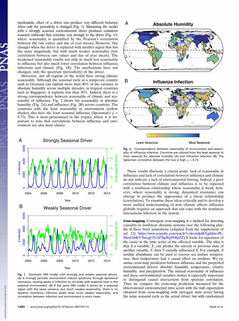
mechanistic effect of a driver can produce very different behaviorwhen only the periodicity is changed (Fig. 1). Simulating the modelwith a strongly seasonal environmental driver produces consistentseasonal outbreaks that correlate very strongly to the driver (Fig. 1A,where seasonality is quantified by the Pearson’s correlationbetween the raw values and day of year mean). However, thischanges when the driver is replaced with another signal that hasthe same magnitude, but with much weaker seasonality (lowcorrelation between raw values and day of year mean). Theweakened seasonality results not only in much less seasonalityin influenza but also much lower correlation between influenzainfections and climate (Fig. 1B). The mechanisms have notchanged, only the spectrum (periodicity) of the driver.Moreover, not all regions of the world have strong climate

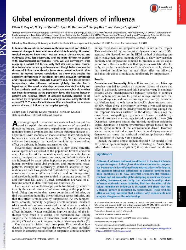
seasonality. Although the seasonal cycle in a temperate countrysuch as Germany can explain more than 90% of the variance inabsolute humidity across multiple decades, in tropical countriessuch as Singapore, it explains less than 30%. Indeed, there is astrong correspondence between seasonality of climate and sea-sonality of influenza. Fig. 2 shows the seasonality in absolutehumidity (Fig. 2A) and influenza (Fig. 2B) across countries. Thecountries with the least seasonality in environment (yellowshades) also have the least seasonal influenza (Spearman’s ρ =0.73). This is most pronounced in the tropics, where it is im-portant to note that correlations between influenza and envi-ronment are also most elusive.

These results illustrate a crucial point: lack of seasonality ininfluenza and lack of correlation between influenza and climatedo not indicate a lack of environmental forcing. Indeed, a poorcorrelation between climate and influenza is to be expectedwith a nonlinear relationship where seasonality is weak; how-ever, where seasonality is strong, dynamical resonance canemerge to produce the appearance of a linear relationship(correlation). To examine these ideas critically and to develop amore unified understanding of how climate affects influenzaglobally requires an approach that can cope with the nonlinearinteractions inherent in the system.

Cross-mapping. Convergent cross-mapping is a method for detectingcausality in nonlinear dynamic systems (see the following play-list of three brief animations (adapted from the supplement ofref. 12): https://www.youtube.com/watch?v=fevurdpiRYg&list=PL-SSmlAMhY3bnogGTe2tf7hpWpl508pZZ).It looks for signatures ofthe cause in the time series of the affected variable. The idea isthat if a variable, X, can predict the current or previous state ofanother variable, Y, then Y causally influenced X. For example, ifsardine abundance can be used to recover sea surface tempera-ture, then temperature had a causal effect on sardines. We ex-amine cross-map prediction between influenza and the purportedenvironmental drivers: absolute humidity, temperature, relativehumidity, and precipitation. The mutual seasonality of influenzaand these environmental variables makes it especially importantto distinguish causal interactions from spurious correlation.Thus, we compare the cross-map prediction measured for theobservational environmental time series with the null expectationobtained from cross-mapping with surrogate time series havingthe same seasonal cycle as the actual driver, but with randomized

Year

2004 2006 2008 2010 2012 2014

020

0040

0060

00

# In

fect

ed

−4

−2

02

4

Env

ironm

enta

l Driv

er

Year

2004 2006 2008 2010 2012 2014

020

0040

0060

00

# In

fect

ed

−4

−2

02

4

Env

ironm

enta

l Driv

er

Strongly Seasonal Driver

Weakly Seasonal Driver

A

B

Fig. 1. Stochastic SIRS model with strongly and weakly seasonal drivers.(A) A strongly periodic environment induces synchrony through dynamicalresonance, causing peaks in infection to correlate with seasonal lows in theseasonal environment. (B) If the same SIRS model is driven by a seasonalsignal with the same variance, but much weaker seasonality, there is nodynamic resonance, infection peaks show much weaker seasonality, andcorrelation between infection and environment is much lower.

Fig. 2. Correspondence between seasonality of environment and season-ality of influenza infection. Countries are colored from the least seasonal tomost seasonal for absolute humidity (A) and influenza infection (B). TheSpearman correlation between the two is high: ρ = 0.73.

13082 | www.pnas.org/cgi/doi/10.1073/pnas.1607747113 Deyle et al.

Dow

nloa

ded

by g

uest

on

Dec

embe

r 26

, 201

9

anomalies. Causal forcing is established when cross-map predic-tion is significantly better for the real environmental driver than itis for the null surrogates (11).Fig. 3 shows box-and-whisker plots of the null distributions for

cross-map skill (ρCCM) ordered according to distance from theequator (absolute latitude). The measured CCM skill values areplotted on top as red circles that are filled if the value is signifi-cantly different from the null distribution (P ≤ 0.05), and openotherwise. Absolute humidity (AH) and temperature (T) bothshow significant forcing in countries across latitude. The resultshave very high metasignificance (Fisher’s method): P < 1.6 × 10−6

for AH and P < 2.9 × 10−3 for T. There is even higher meta-significant evidence for forcing across latitudes by relativehumidity: P < 1.8 × 10−14. However, paired Wilcox tests (non-parametric generalization of Student’s t test) in the predictionskill confirm that the cross-map effect with respect to RH isweaker on average than with either AH or T (P < 0.02), but thatthe strength of effects of AH and T are not significantly differentfrom one another. Finally, there is some evidence that pre-cipitation may be a causal variable in a few countries (globalmetasignificance, P < 7.3 × 10−3; tropics only, P < 0.023).If all other things are equal, the magnitude of cross-map skill

(ρCCM) can indicate the strength of causal effect. On this basis,one might conclude that because the absolute level of cross-mapskill is lower in the tropics, the causal effect of climate (absolutehumidity or temperature) is weaker. However, this would beincorrect, as “all things equal” does not apply across latitudesbecause of the differences in seasonality, and hence differencesin the baseline predictability in these systems. This dichotomyis illustrated with the model shown in Fig. 1. Both model realiza-tions have the same ultimate magnitude of the effect of AH on flu.

In Fig. 1A, however, the driver has much stronger seasonality, andis therefore more predictable. The seasonal cycle, being identicalfrom year to year, is trivial to predict; meaning the stronger theeffect of the seasonal cycle, the easier the driver is to predict. Thus,the absolute level of ρCCM is substantially higher in Fig. 1A thanFig. 1B, even though the strength of causal effect is likely un-changed. Therefore, in this case, the skill of CCM (ρCCM) shouldnot be used as a relative measure of causal strength when com-paring CCM across latitudes, as the climate time series in tropicaland temperate countries do not have the same basic levels ofpredictability.

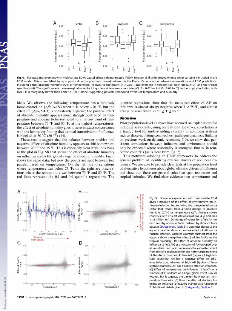
Multivariate EDM. To examine whether AH or T has a strongercausal effect on influenza according to previous work (12), weuse a multivariate EDM approach that looks for improvement inforecasting when a suspected causal variable is included. In brief,if a multivariate empirical dynamic model containing a potentialdriving variable Y produces better forecasts of X than without,then Y causally influenced X. The results are summarized in Fig.4. The results show strong evidence that AH and T are drivers ofinfluenza, as including either variable leads to improved forecastskill (P < 0.001 globally). However, in the tropics (where AH andT generally have weaker correlation), we find that including AHand T together as embedding coordinates leads to slightly moreimprovement over either one alone. In temperate countries, wherecorrelations between AH and T are extremely high (generally >0.9), these variables contain almost identical information, andhence there is less difference in forecast skill on average betweenembeddings with AH, T, or both. Overall, multivariate forecastimprovement suggests the possibility that AH and T taken to-gether have a nonlinear effect on influenza that is global, but thatthis effect is concealed in the temperate region by their strongcorrelation to each other.To explore the mechanism for this interaction further, we

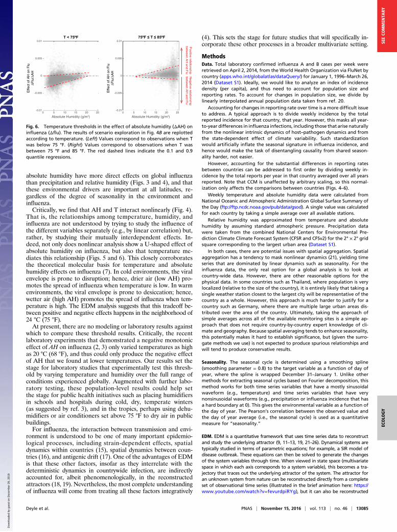
predict the hypothetical change in influenza incidence, denotedΔflu, at historical points that would occur from small increasesand decreases in the environmental driver [EDM scenario ex-ploration (13)]. This simple device allows us not only to directlyquantify the magnitude and direction of effect but also to keeptrack of how the effect changes through time and with varyingenvironmental conditions. Fig. 5A shows country by country themagnitude of the effect of absolute humidity on influenza, Δflu/ΔAH. Countries at high latitudes generally show a negative effectof absolute humidity on influenza, whereas low-latitude coun-tries generally show a positive effect. This is consistent with thehypothesized U-shaped response of influenza to AH suggestedby certain experiments (8).We can examine this effect further by plotting the scenario

exploration results for all the countries together. Fig. 5B showsthat the effect of AH on influenza is negative at low AH (Δflu/ΔAH < 0), but positive at high AH (Δflu/ΔAH > 0), consistentwith a U-shaped response of influenza survival to absolute hu-midity. The negative effect on incidence at low AH and positiveeffect at high AH appear roughly equivalent when the data arenormalized to average total reported cases in a year in thatcountry.The same analysis for temperature (Fig. 5C) does not exhibit

such a clear state-dependent (nonlinear) effect. Temperaturechanges can have a positive (Δflu/ΔT > 0) or negative (Δflu/ΔT <0) effect on influenza at the same temperature. Indeed, the mo-lecular arguments for a U-shaped effect of absolute humidity oninfluenza also predict that temperature should be a control onthe balance between the positive and negative effects of absolutehumidity (7).With this in mind, we look at the effect of absolute humidity

on influenza (Δflu/ΔAH) as a function of temperature (Fig. 5D).This is perhaps the most interesting picture to emerge, as thereare a number of features that corroborate and elaborate existing

AbsoluteHumidity

Temperature RelativeHumidity

Precipitation

FinlandNorwaySweden

LatviaDenmark

United KingdomPoland

GermanySwitzerland

SloveniaFrance

RomaniaSpain

PortugalJapanChile

South AfricaParaguay

New CaledoniaMadagascar

ThailandSenegal

PhilippinesPeru

ColombiaMalaysia

0 0.5 1 0 0.5 1 0 0.5 1 0 0.5 1

distance from equator

Fig. 3. Detecting cross-map causality beyond shared seasonality of envi-ronmental drivers on influenza. Red circles show the unlagged cross-mapskill (ρCCM) for observed influenza predicting purported seasonal drivers:absolute humidity, temperature, relative humidity, and precipitation. To-gether with this, box-and-whisker plots show the null distributions for ρCCMexpected from random surrogate time series that shares the same season-ality as the true environmental driver. Countries are ordered according todistance from the equator (absolute latitude). Filled circles indicate that themeasured ρCCM is significantly better than the null expectation (P ≤ 0.05).

Deyle et al. PNAS | November 15, 2016 | vol. 113 | no. 46 | 13083

ECOLO

GY

SEECO

MMEN

TARY

Dow

nloa

ded

by g

uest

on

Dec

embe

r 26

, 201

9

ideas. We observe the following: temperature has a relativelyloose control on (Δflu/ΔAH) when it is below ∼70 °F, but theeffect on (Δflu/ΔAH) is consistently negative; the positive effectof absolute humidity appears more strongly controlled by tem-perature and appears to be restricted to a narrow band of tem-perature between 75 °F and 85 °F; at the highest temperatures,the effect of absolute humidity goes to zero in exact concordancewith the laboratory finding that aerosol transmission of influenzais blocked at 30 °C (86 °F) (14).These results suggest that the balance between positive and

negative effects of absolute humidity appears to shift somewherebetween 70 °F and 75 °F. This is especially clear if we look backat the plot in Fig. 5B that shows the effect of absolute humidityon influenza across the global range of absolute humidity. Fig. 6shows the same data, but now the points are split between twopanels, based on temperature. On the left are observationswhere temperature was below 75 °F; on the right are observa-tions where the temperature was between 75 °F and 85 °F. Thered lines represent the 0.1 and 0.9 quantile regressions. The

quantile regressions show that the measured effect of AH oninfluenza is almost always negative when T < 75 °F, and almostalways positive when 75 °F ≤ T ≤ 85 °F.

DiscussionPrior population-level analyses have focused on explanations forinfluenza seasonality, using correlations. However, correlation isa limited tool for understanding causality in nonlinear systemssuch as those exhibiting complex host–pathogen dynamics. Buildingon previous work on dynamic resonance (10), we show that per-sistent correlations between influenza and environment shouldonly be expected where seasonality is strongest; that is, in tem-perate countries (as is clear from Fig. 2).This motivates adopting an EDM framework to address the

general problem of identifying external drivers of nonlinear dy-namics. We are able to provide clear tests at the population levelof alternative hypotheses about global climatic drivers of influenzaand show that there are general rules that span temperate andtropical latitudes. We find clear evidence that temperature and

−0.06

−0.03

0.00

0.03

0.06

AH T

RH

Prc

p

AH

+T

For

ecas

t Im

prov

emen

t (

)

Global

−0.06

−0.03

0.00

0.03

0.06

AH T

RH

Prc

p

AH

+T

For

ecas

t Im

prov

emen

t (

)

Tropical

−0.06

−0.03

0.00

0.03

0.06

AH T

RH

Prc

p

AH

+T

For

ecas

t Im

prov

emen

t (

)

TemperateBA C

Fig. 4. Forecast improvement with multivariate EDM. Causal effect is demonstrated if EDM forecast skill (ρ) improves when a driver variable is included in theEDM model. This is quantified by Δρ = ρ(with driver) − ρ(without driver), where ρ is the Pearson’s correlation between observations and EDM predictions.Including either absolute humidity (AH) or temperature (T) leads to significant (P < 0.001) improvement in forecast skill both globally (A) and the tropicsspecifically (B). The significance is more marginal when looking solely at temperate countries (C) (P < 0.07 for AH; P < 0.03 for T). In the tropics, including both(AH +T) is marginally better than either AH or T alone, suggesting possible compound effects of temperature and humidity.

Temperature T20 40 60 80 100

Effe

ct o

f AH

on

Flu

Flu

/AH

-0.01

-0.005

0

0.005

0.01

Absolute Humidity AH0 10 15 20 25

Effe

ct o

f AH

on

Flu

Flu

/AH

-0.01

-0.005

0

0.005

0.01

5

Temperature T20 40 60 80 100

Effe

ct o

f T o

n F

luF

lu/T

-0.01

-0.005

0

0.005

0.01

Effe

ct o

f AH

on

Flu

Flu

/AH

-0.01

-0.005

0

0.005

0.01

10 20 30 40 50 60

Country (ranked by |Lat|)

DistanceFrom Equator

Positive relationship

between A

H and F

luN

egative relationshipbetw

een AH

and Flu

A B

C D

Fig. 5. Scenario exploration with multivariate EDMgives a measure of the effect of environment on in-fluenza infection by predicting the change in influenza(Δflu) that results from a small change in absolutehumidity (ΔAH) or temperature (ΔT). Analysis coverscountries with at least 208 observations (4 y) and area<1.5 million mi2. (A) Range of values for Δflu/ΔAH foreach country across latitude, ordered by distance fromequator (SI Appendix, Table S1). Countries closest to theequator tend to show a positive effect of AH on in-fluenza infection, whereas countries furthest from theequator show a negative effect (red line indicates thetropical boundary). (B) Effect of absolute humidity oninfluenza (Δflu/ΔAH) as a function of AH grouped overall countries. Each point represents the estimated effectfrom scenario exploration for one historical point in oneof the study countries. At low AH (typical of high-lati-tude countries), AH has a negative effect on influ-enza infection, whereas at high AH (typical of low-latitude countries), AH has a positive effect on influenza.(C) Effect of temperature on influenza (Δflu/ΔT) as afunction of T. Evidence of a single global effect is muchweaker, but it suggests there might be important tem-perature thresholds. (D) How the effect of absolute hu-midity on influenza (Δflu/ΔAH) changes as a function ofT. Additional details given in SI Appendix, Section 5.

13084 | www.pnas.org/cgi/doi/10.1073/pnas.1607747113 Deyle et al.

Dow

nloa

ded

by g

uest

on

Dec

embe

r 26

, 201

9

absolute humidity have more direct effects on global influenzathan precipitation and relative humidity (Figs. 3 and 4), and thatthese environmental drivers are important at all latitudes, re-gardless of the degree of seasonality in the environment andinfluenza.Critically, we find that AH and T interact nonlinearly (Fig. 4).

That is, the relationships among temperature, humidity, andinfluenza are not understood by trying to study the influence ofthe different variables separately (e.g., by linear correlation) but,rather, by studying their mutually interdependent effects. In-deed, not only does nonlinear analysis show a U-shaped effect ofabsolute humidity on influenza, but also that temperature me-diates this relationship (Figs. 5 and 6). This closely corroboratesthe theoretical molecular basis for temperature and absolutehumidity effects on influenza (7). In cold environments, the viralenvelope is prone to disruption; hence, drier air (low AH) pro-motes the spread of influenza when temperature is low. In warmenvironments, the viral envelope is prone to desiccation; hence,wetter air (high AH) promotes the spread of influenza when tem-perature is high. The EDM analysis suggests that this tradeoff be-tween positive and negative effects happens in the neighborhood of24 °C (75 °F).At present, there are no modeling or laboratory results against

which to compare these threshold results. Critically, the recentlaboratory experiments that demonstrated a negative monotoniceffect of AH on influenza (2, 3) only varied temperatures as highas 20 °C (68 °F), and thus could only produce the negative effectof AH that we found at lower temperatures. Our results set thestage for laboratory studies that experimentally test this thresh-old by varying temperature and humidity over the full range ofconditions experienced globally. Augmented with further labo-ratory testing, these population-level results could help setthe stage for public health initiatives such as placing humidifiersin schools and hospitals during cold, dry, temperate winters(as suggested by ref. 3), and in the tropics, perhaps using dehu-midifiers or air conditioners set above 75 °F to dry air in publicbuildings.For influenza, the interaction between transmission and envi-

ronment is understood to be one of many important epidemio-logical processes, including strain-dependent effects, spatialdynamics within countries (15), spatial dynamics between coun-tries (16), and antigenic drift (17). One of the advantages of EDMis that these other factors, insofar as they interrelate with thedeterministic dynamics in countrywide infection, are indirectlyaccounted for, albeit phenomenologically, in the reconstructedattractors (18, 19). Nevertheless, the most complete understandingof influenza will come from treating all these factors integratively

(4). This sets the stage for future studies that will specifically in-corporate these other processes in a broader multivariate setting.

MethodsData. Total laboratory confirmed influenza A and B cases per week wereretrieved on April 2, 2014, from the World Health Organization via FluNet bycountry (apps.who.int/globalatlas/dataQuery/) for January 1, 1996–March 26,2014 (Dataset S1). Ideally, we would like to analyze an index of incidencedensity (per capita), and thus need to account for population size andreporting rates. To account for changes in population size, we divide bylinearly interpolated annual population data taken from ref. 20.

Accounting for changes in reporting rate over time is a more difficult issueto address. A typical approach is to divide weekly incidence by the totalreported incidence for that country, that year. However, this masks all year-to-year differences in influenza infections, including those that arise naturallyfrom the nonlinear intrinsic dynamics of host–pathogen dynamics and fromthe state-dependent effect of climate variability. Such standardizationwould artificially inflate the seasonal signature in influenza incidence, andhence would make the task of disentangling causality from shared season-ality harder, not easier.

However, accounting for the substantial differences in reporting ratesbetween countries can be addressed to first order by dividing weekly in-cidence by the total reports per year in that country averaged over all yearsreported. Note that CCM is unaffected by arbitrary scaling, so this normal-ization only affects the comparisons between countries (Figs. 4–6).

Weekly temperature and absolute humidity data were calculated fromNational Oceanic and Atmospheric Administration Global Surface Summary ofthe Day (ftp://ftp.ncdc.noaa.gov/pub/data/gsod). A single value was calculatedfor each country by taking a simple average over all available stations.

Relative humidity was approximated from temperature and absolutehumidity by assuming standard atmospheric pressure. Precipitation datawere taken from the combined National Centers for Environmental Pre-diction Climate Climate Forecast System (CFSR and CFSv2) for the 2° × 2° gridsquare corresponding to the largest urban area (Dataset S1).

In both cases, there are potential issues with spatial aggregation. Spatialaggregation has a tendency to mask nonlinear dynamics (21), yielding timeseries that are dominated by linear dynamics such as seasonality. For theinfluenza data, the only real option for a global analysis is to look atcountry-wide data. However, there are other reasonable options for thephysical data. In some countries such as Thailand, where population is verylocalized (relative to the size of the country), it is entirely likely that taking asingle weather station closest to the largest city will be representative of thecountry as a whole. However, this approach is much harder to justify for acountry such as Germany, where there are multiple large urban areas dis-tributed over the area of the country. Ultimately, taking the approach ofsimple averages across all of the available monitoring sites is a simple ap-proach that does not require country-by-country expert knowledge of cli-mate and geography. Because spatial averaging tends to enhance seasonality,this potentially makes it hard to establish significance, but (given the surro-gate methods we use) is not expected to produce spurious relationships andwill tend to produce conservative results.

Seasonality. The seasonal cycle is determined using a smoothing spline(smoothing parameter = 0.8) to the target variable as a function of day ofyear, where the spline is wrapped December 31–January 1. Unlike othermethods for extracting seasonal cycles based on Fourier decomposition, thismethod works for both time series variables that have a mostly sinusoidalwaveform (e.g., temperature) and time series variables that have verynonsinusoidal waveforms (e.g., precipitation or influenza incidence that hasa hard boundary at 0). This gives the environmental variable as a function ofthe day of year. The Pearson’s correlation between the observed value andthe day of year average (i.e., the seasonal cycle) is used as a quantitativemeasure for “seasonality.”

EDM. EDM is a quantitative framework that uses time series data to reconstructand study the underlying attractor (9, 11–13, 19, 21–26). Dynamical systems aretypically studied in terms of parametric equations; for example, a SIR model ofdisease outbreak. These equations can then be solved to generate the changesof the system variables through time. When viewed in state space (multivariatespace in which each axis corresponds to a system variable), this becomes a tra-jectory that traces out the underlying attractor of the system. The attractor foran unknown system from nature can be reconstructed directly from a completeset of observational time series (illustrated in the brief animation here: https://www.youtube.com/watch?v=fevurdpiRYg), but it can also be reconstructed

Absolute Humidity (g/m3)0 5 10 15 20 25

Effe

ct o

f AH

on

Flu

ΔFlu

/ΔA

H

Effe

ct o

f AH

on

Flu

ΔFlu

/ΔA

H

-0.01

-0.005

0

0.005

0.01

Absolute Humidity (g/m3)0 5 10 15 20 25

-0.01

-0.005

0

0.005

0.01

Positive relationship

between A

H and F

luN

egative relationshipbetw

een AH

and Flu

T < 75ºF 75ºF ≤ T ≤ 85ºF

Fig. 6. Temperature thresholds in the effect of absolute humidity (ΔAH) oninfluenza (Δflu). The results of scenario exploration in Fig. 4B are replottedaccording to temperature. (Left) Values correspond to observations when Twas below 75 °F. (Right) Values correspond to observations when T wasbetween 75 °F and 85 °F. The red dashed lines indicate the 0.1 and 0.9quantile regressions.

Deyle et al. PNAS | November 15, 2016 | vol. 113 | no. 46 | 13085

ECOLO

GY

SEECO

MMEN

TARY

Dow

nloa

ded

by g

uest

on

Dec

embe

r 26

, 201

9

from a single time series by using time-lagged coordinates (https://www.youtube.com/watch?v=QQwtrWBwxQg). The dynamic attractor is a completerepresentation of the system, and thus can be studied in place of parametricequations to predict and understand systems such as host–pathogen dynamics.

This general framework can be applied in a number of ways—to detectcausation (9), forecast future states (22, 23), track interactions (24), and so on—using the R package “rEDM” (https://cran.r-project.org/web/packages/rEDM/index.html), which includes a technical description of the methods in a vignette(https://cran.r-project.org/web/packages/rEDM/vignettes/rEDM_tutorial.htmldocumentation). Additional details on the exact calculations are given here.Note that EDM prediction skill in this article is always measured with Pearson’scorrelation (ρ) between observed and predicted values.

CCM Analysis and Seasonal Surrogates. The basic idea of convergent cross-mapping is to use prediction between variables as a test for causality. Ifvariable Y had a causal effect on variable X, then causal information ofvariable Y should be present in X, and so the attractor recovered for variableX should be able to predict the states of variable Y (https://www.youtube.com/watch?v=iSttQwb-_5Y).

For basic CCM analysis, we use simplex projection, which has a single pa-rameter to select: the embedding dimension E. As in ref. 24, we select E on thebasis of the optimal prediction of cross-mapping lagged 1 wk, then measurethe unlagged cross-map skill with this value of E. Some of the influenza timeseries have long stretches of zero-values, which will contain little or no in-formation about the climate. As a consequence, we exclude from the pre-diction set all stretches of zeros at least 8 time points long (the maximumembedding dimension tested) to improve the sensitivity of the analysis.

Checking for convergence in cross-map skill (i.e., that cross-map skill im-proves with the amount of data used) is a general way to distinguish cross-mapping from spurious correlation (9). However, we are concerned herewith a more specific problem of distinguishing driving effects from mutualseasonality. This is more directly addressed by developing a null test withsurrogate time series, in the vein of ref. 11.

For a forcing variable Z(t) (e.g., absolute humidity or temperature), wecalculate the day of year average Z (i.e., the seasonal cycle) as earlier, and theseasonal anomaly as the difference between the observed value Z(t) and theday of year average for that day, ~ZðtÞ= ZðtÞ-ZðtÞ. We then randomly shuffle(permute) the time indices of the seasonal anomalies. Adding the shuffledanomalies back to the season average gives a surrogate time series Z* that hasthe same seasonal average as Z, but with random anomalies. If Z is in fact adriver of influenza, then influenza will be sensitive not only to the seasonalcomponent of Z but also to the anomalies. Thus, influenza should betterpredict the real time series Z than the surrogate Z*. In practice, we repeat theshuffling procedure 500 times to produce an ensemble of surrogates.

Note that in determining the metasignificance of the CCM tests, we applyFisher’s method, which relies on the assumption that the different P valuesare independent. However, both influenza epidemics and climate havespatial dependencies between countries. Because there is no practical way todetermine the covariance between P values in this experiment, Fisher’smethod is the best guide, but it is important to note that the meta-significance may be somewhat anticonservative.

Multivariate EDM: Forecast Improvement.When driver variables are stochastic(e.g., seasonal anomalies of climactic variables), multivariate forecast im-provement can be used as a test for causality (12). A stochastic variable isconsidered causal if explicitly including it as a coordinate in the state spaceleads to improved nearest-neighbor forecasts. In the case of seasonal in-fluenza, however, we cannot necessarily treat the environmental time seriesas stochastic variables. This means that information about the drivers is al-ready contained in the univariate embedding (9, 25). Thus, we modify themethod of ref. 12 as follows.

We determine the optimal univariate embedding dimension, E*, for eachinfluenza time series, following ref. 26. A univariate embedding with di-mension E < E* will be “under embedded”; that is, it will not contain fullinformation about the system state and dynamics. In this case, incorporatinginformation about a driver in a multivariate embedding will generally leadto an increase in forecast skill. Thus, we calculate the improvement inforecast skill, using simplex projection of the univariate embedding with E =E*−1 and the same embedding, but with the candidate environmentalvariable(s) included as a coordinate. As with CCM, we exclude all stretches ofzeros at least eight time points long (maximum tested E) from the predictionset to improve the sensitivity of the analysis. Significant improvement iscalculated using a one-sample Wilcox test (nonparametric Student’s t test),and significant differences in the improvement between variables is calcu-lated using a paired two-sample Wilcox test.

Multivariate EDM: Scenario Exploration. Multivariate scenario exploration is away to empirically assess the effect of a small change in a physical driver (e.g.,absolutehumidity) on influenza incidence.Wepredict theeffect of a small increasein absolute humidity or temperature on influenza 2 wk later to understand thesensitivity of influenza outbreaks to the environment. For each historical timepoint, t, we predict influenza with a small increase (+ΔZ/2) and a small decrease(−ΔZ/2) in historically measured driver Z(t). The difference in predicted influenza isΔflu = flut+1[Z = Z(t)+ΔZ/2] – flut+2[Z = Z(t) – ΔZ/2], and the ratio of Δflu/ΔZquantifies the sensitivity of influenza infection to the driver Z at time t. We useΔZ = 0.2 g/m3 and 0.5 °F for absolute humidity and temperature, respectively.These values correspond to∼5%of the SD of these variables across all of the countriesanalyzed. Forecasts were performed using S-maps (22), with E = 7 and θ = 0.9.

1. Xie X, Li Y, Chwang ATY, Ho PL, Seto WH (2007) How far droplets can move in indoorenvironments–Revisiting the Wells evaporation-falling curve. Indoor Air 17(3):211–225.

2. Lowen AC, Mubareka S, Steel J, Palese P (2007) Influenza virus transmission is de-pendent on relative humidity and temperature. PLoS Pathog 3(10):1470–1476.

3. Shaman J, Kohn M (2009) Absolute humidity modulates influenza survival, trans-mission, and seasonality. Proc Natl Acad Sci USA 106(9):3243–3248.

4. Lofgren E, Fefferman NH, Naumov YN, Gorski J, Naumova EN (2007) Influenza sea-sonality: Underlying causes and modeling theories. J Virol 81(11):5429–5436.

5. Tamerius JD, et al. (2013) Environmental predictors of seasonal influenza epidemicsacross temperate and tropical climates. PLoS Pathog 9(3):e1003194.

6. Shaman J, Pitzer VE, Viboud C, Grenfell BT, Lipsitch M (2010) Absolute humidity andthe seasonal onset of influenza in the continental United States. PLoS Biol 8(2):e1000316.

7. Minhaz Ud-Dean SM (2010) Structural explanation for the effect of humidity onpersistence of airborne virus: Seasonality of influenza. J Theor Biol 264(3):822–829.

8. Schaffer FL, Soergel ME, Straube DC (1976) Survival of airborne influenza virus: Effectsof propagating host, relative humidity, and composition of spray fluids. Arch Virol51(4):263–273.

9. Sugihara G, et al. (2012) Detecting causality in complex ecosystems. Science 338(6106):496–500.

10. Dushoff J, Plotkin JB, Levin SA, Earn DJD (2004) Dynamical resonance can account forseasonality of influenza epidemics. Proc Natl Acad Sci USA 101(48):16915–16916.

11. Tsonis AA, et al. (2015) Dynamical evidence for causality between galactic cosmic raysand interannual variation in global temperature. Proc Natl Acad Sci USA 112(11):3253–3256.

12. Dixon PA, Milicich MJ, Sugihara G (1999) Episodic fluctuations in larval supply. Science283(5407):1528–1530.

13. Deyle ER, et al. (2013) Predicting climate effects on Pacific sardine. Proc Natl Acad SciUSA 110(16):6430–6435.

14. Lowen AC, Steel J, Mubareka S, Palese P (2008) High temperature (30 degrees C) blocks

aerosol but not contact transmission of influenza virus. J Virol 82(11):5650–5652.15. Viboud C, et al. (2006) Synchrony, waves, and spatial hierarchies in the spread of

influenza. Science 312(5772):447–451.16. Russell CA, et al. (2008) The global circulation of seasonal influenza A (H3N2) viruses.

Science 320(5874):340–346.17. Smith DJ, et al. (2004) Mapping the antigenic and genetic evolution of influenza vi-

rus. Science 305(5682):371–376.18. Takens F (1981) Detecting strange attractors in turbulence. Dynamical Systems and

Turbulence, Warwick 1980, eds Rand DA, Young L (Lector Notes in Mathematics, New

York), pp 366–381.19. Ye H, et al. (2015) Equation-free mechanistic ecosystem forecasting using empirical

dynamic modeling. Proc Natl Acad Sci USA 112(13):E1569–E1576.20. The World Bank (2015) Health Nutrition and Population Statistics. Available at data.

worldbank.org/indicator/SP.POP.TOTL. Accessed April 4, 2014.21. Sugihara G, Grenfell B, May RM (1990) Distinguishing error from chaos in ecological

time series. Philos Trans R Soc Lond B Biol Sci 330(1257):235–251.22. Sugihara G, May RM (1990) Nonlinear forecasting as a way of distinguishing chaos

from measurement error in time series. Nature 344(6268):734–741.23. Sugihara G (1994) Nonlinear forecasting for the classification of natural time series.

Philos T Roy Soc A 348(1688):477–495.24. Deyle ER, May RM, Munch SB, Sugihara G (2016) Tracking and forecasting ecosystem

interactions in real time. Proc Biol Sci 283(1822):20152258.25. Stark J, Broomhead DS, Davies ME, Huke J (2003) Delay embeddings for forced sys-

tems. II. Stochastic forcing. J Nonlinear Sci 13(6):519–577.26. Glaser SM, et al. (2014) Complex dynamics may limit prediction in marine fisheries.

Fish Fish 15(4):616–633.

13086 | www.pnas.org/cgi/doi/10.1073/pnas.1607747113 Deyle et al.

Dow

nloa

ded

by g

uest

on

Dec

embe

r 26

, 201

9