Global Energy-saving Map of StrongOcean Currents

Yu-Chia Chang1, Ruo-Shan Tseng2, Peter C Chu3 and Huan-Jie Shao1

1(Department of Marine Biotechnology and Resources, National Sun Yat-sen University,Kaohsiung 80424, Taiwan)

2(Department of Oceanography, National Sun Yat-sen University,Kaohsiung 80424, Taiwan)

3(Department of Oceanography, Naval Postgraduate School, Monterey,CA 93943, USA)

(E-mail: rstseng@mail.nsysu.edu.tw)

This study provides a global, detailed, and complete energy-saving map of strong ocean cur-rents from the absolute geostrophic velocities calculated from satellite altimetry data, with thefocus on the strong Western Boundary Currents (WBCs) in the global ocean. Theoretically,the WBCs with speeds of 2–3 knots can reduce fuel consumption by 25–50% for vessels ata sailing speed of 6 knots. The fuel savings are greater for a lower sailing speed than for ahigher sailing speed. For about 1·8 million motorised fishing vessels with a lower shipspeed, strong currents can evidently save fuel, time and money. Since global fishing vesselsgenerate roughly 130 million tonnes of CO2 per annum (FAO, 2012), effective utilisation ofthe energy-saving map could significantly reduce CO2 emissions from ship operations.

KEY WORDS

1. Vessel. 2. Current. 3. Energy-saving. 4. Route.

Submitted: 8 April 2014. Accepted: 20 May 2015.

1. INTRODUCTION. According to the InternationalMaritimeOrganization (IMO,2009a) andFoodandAgricultureOrganization of theUnitedNations (FAO, 2012), global-ly, there were around 70 000 merchant ships sailing for world trade and about 4·36 millionfishing vessels with nearly 2·6 million engine-powered in 2010. Among the motorisedfishing vessels, about 1·8 million were operated in sea waters and others were operated ininland waters. In 1997, the IMO adopted a resolution on CO2 emissions from ships.Afterwards, the Marine Environment Protection Committee (MEPC) developed a green-house gas emission index for ships (IMO, 2009a). The MEPC published guidelines forthe use of an Energy EfficiencyOperational Indicator (EEOI), which provides useful infor-mation on ship’s performance with regard to fuel efficiency. The EEOI is currently for vol-untary use by each ship. Recently, the IMO (2012) has started to require the EnergyEfficiency Design Index (EEDI) for new ships, and the Ship Energy EfficiencyManagement Plan (SEEMP) for all ships. These documents list various options to

THE JOURNAL OF NAVIGATION, Page 1 of 18. © The Royal Institute of Navigation 2015doi:10.1017/S0373463315000466

Report Documentation Page Form ApprovedOMB No. 0704-0188

Public reporting burden for the collection of information is estimated to average 1 hour per response, including the time for reviewing instructions, searching existing data sources, gathering andmaintaining the data needed, and completing and reviewing the collection of information. Send comments regarding this burden estimate or any other aspect of this collection of information,including suggestions for reducing this burden, to Washington Headquarters Services, Directorate for Information Operations and Reports, 1215 Jefferson Davis Highway, Suite 1204, ArlingtonVA 22202-4302. Respondents should be aware that notwithstanding any other provision of law, no person shall be subject to a penalty for failing to comply with a collection of information if itdoes not display a currently valid OMB control number.

1. REPORT DATE 2015 2. REPORT TYPE

3. DATES COVERED 00-00-2015 to 00-00-2015

4. TITLE AND SUBTITLE Global Energy-saving Map of Strong Ocean Currents

5a. CONTRACT NUMBER

5b. GRANT NUMBER

5c. PROGRAM ELEMENT NUMBER

6. AUTHOR(S) 5d. PROJECT NUMBER

5e. TASK NUMBER

5f. WORK UNIT NUMBER

7. PERFORMING ORGANIZATION NAME(S) AND ADDRESS(ES) Naval Postgraduate School,Department of Oceanography,Monterey,CA,93943

8. PERFORMING ORGANIZATIONREPORT NUMBER

9. SPONSORING/MONITORING AGENCY NAME(S) AND ADDRESS(ES) 10. SPONSOR/MONITOR’S ACRONYM(S)

11. SPONSOR/MONITOR’S REPORT NUMBER(S)

12. DISTRIBUTION/AVAILABILITY STATEMENT Approved for public release; distribution unlimited

13. SUPPLEMENTARY NOTES

14. ABSTRACT This study provides a global, detailed, and complete energy-saving map of strong ocean currents from theabsolute geostrophic velocities calculated from satellite altimetry data, with the focus on the strongWestern Boundary Currents (WBCs) in the global ocean. Theoretically the WBCs with speeds of 2???3knots can reduce fuel consumption by 25???50% for vessels at a sailing speed of 6 knots. The fuel savingsare greater for a lower sailing speed than for a higher sailing speed. For about 1??8 million motorisedfishing vessels with a lower ship speed, strong currents can evidently save fuel, time and money. Sinceglobal fishing vessels generate roughly 130 million tonnes of CO2 per annum (FAO, 2012), effectiveutilisation of the energy-saving map could significantly reduce CO2 emissions from ship operations.

15. SUBJECT TERMS

16. SECURITY CLASSIFICATION OF: 17. LIMITATION OF ABSTRACT Same as

Report (SAR)

18. NUMBEROF PAGES

18

19a. NAME OFRESPONSIBLE PERSON

a. REPORT unclassified

b. ABSTRACT unclassified

c. THIS PAGE unclassified

Standard Form 298 (Rev. 8-98) Prescribed by ANSI Std Z39-18

improve energy efficiency such as speed optimisation, weather routing, and hull mainten-ance (IMO, 2012). The optimum speed represents the speed at which minimum fuelusage per tonnagemile is reached. Speed optimisation canyield significant savings and con-sideration of the enginemanufacturer’s power curve and the ship’s propeller curve should beincorporated.Generally, a 10%decrease of ship speedwill result in 19% reduction of enginepower and 27% reduction of energy consumption and therefore reduction inCO2 emissions(IMO, 2010). Weather routing is available for all types of ship, and has a high potential forenergy efficiency. Ship routing often considers oceanweather associatedwith eddies, mean-ders, storm likelihood, ocean surface waves, sea ice and tides. Optimising ship routes notonly reduces CO2 emissions but also reduces emissions of NOx, black carbon and SO2,which will impact on climate and health. For hull maintenance, the smoother the hull,the better fuel efficiency. Propeller cleaning and polishing can significantly increase fuel ef-ficiency.According to IMO(2009a; 2009b; 2011), other technologies are also expected tobeused for reducing fuel consumption such as improvement of engine efficiency, reducing on-board power demand, optimisation of ship handling, solar power, and wind power, etc.Application of favourable ocean currents can also reduce a ship’s energy consump-

tion (Lo and McCord, 1995; Chang et al., 2013b). Usually, strong ocean currents existnear the western boundary of ocean basins, and are called the Western BoundaryCurrents (WBCs) such as the Gulf Stream in the North Atlantic and the Kuroshioin the North Pacific. In addition, swift surface flows can be sometimes induced byhigh wind speeds or tropical cyclones (Chang et al., 2010; 2012; 2013a). Lo andMcCord (1995) estimated that 5–8% fuel savings can be achieved for ships travelingwith the Gulf Stream at sailing speeds of about 16 knots. Chang et al. (2013b) sug-gested a fuel reduction of 2–6% for vessels sailing with the Kuroshio Currentbetween Taipei and Tokyo at an average speed of 12 knots. Effective use of thesestrong currents can yield huge savings considering that a large number of engine-powered fishing boats worldwide move at speeds of about 6–10 knots. The energysavings are even more obvious for ships with a lower cruising speed when takinginto account strong ocean currents. The typical flow speeds of WBCs are approximate-ly 2–3 knots, which is equivalent to 33–50% of the ship speeds of small fishing boats.Thus, smaller fishing boats will save more fuel, time and money, and reduce green-house gas emissions if they effectively utilise strong ocean currents. Questions arise:Do captains of all vessels know the correct locations of these strong currents foroptimal route planning? Can a global map of strong currents be constructed from arelatively long time series of current data? How significant is the fuel saving afterthe detailed ocean circulation mapping is constructed and utilised? The goal of thisstudy is to answer these questions, and to provide an energy-saving map with strongcurrents for all types of ships. The study will also focus on ship’s characteristics topresent the impact on navigation (i.e. ship’s particulars) based on strong ocean cur-rents. To do so, global current data from satellite measurements are used to representa detailed and complete map of strong currents.

2. DATA. In this study, geostrophic currents of 1992–2012 from amerged product ofTOPEX/Poseidon, Jason 1, and European Research Satellite altimeter observations areused to examine the global ocean surface circulation. Produced by the French Archiving,Validation, and Interpolation of Satellite Oceanographic Data (AVISO) project usingthe mapping method of Ducet et al. (2000), the total geostrophic currents can be

2 YU-CHIA CHANG AND OTHERS

obtained from the AVISO website (http://www.aviso.oceanobs.com/index.php?id=1271).The data processing of AVISO using optimal interpolation with realistic correlationfunctions generates a combined map merging measurements from all available altimetermissions (Ducet et al., 2000). The combined data from all altimeter missions can greatlyimprove the estimation of mesoscale signals. The data are interpolated onto a global gridof 1/3° resolution between 82°S and 82°N and are archived in weekly (7 days) averagedframes. The geostrophic currents are calculated from the absolute dynamic topography,which consists of a Mean Dynamic Topography (MDT) and the anomalies of the altim-eter sea level. Rio and Hernandez (2004) have explained in detail the method of estimat-ing the MDT. The resulting geostrophic currents have been validated with independentdrifter data to have a root-mean-square difference of about 14 cm/s in the Kuroshio area(Rio andHernandez, 2004). Readers are referred to Le Traon et al. (1998), Le Traon andDibarbour (1999), Le Traon et al. (2001), Pascual et al. (2006), Ducet et al. (2000) andQiu and Chen (2006) for more details on the data analysis method.

3. GLOBAL STRONG OCEAN CURRENTS. Figure 1 shows the global oceanbathymetry derived from ETOPO2. The mean current speeds and vectors averagedfrom AVISO data of 1992–2012 in 1/3° × 1/3° bins are shown in Figures 2 and 3, re-spectively. Strong currents (∼2 knots) can be clearly seen to occur in the six redboxes of Figure 2 (marked as a-f), with their locations at the North America, SouthAmerica, Northeast Asia, Southeast Asia, Australia, and Africa, respectively. Mostof the strong currents are typical WBCs in the Pacific, Atlantic and Indian Ocean.

Figure 1. Geography and bottom topography of the world oceans derived from ETOPO2.

3GLOBAL ENERGY-SAVING MAP OF STRONG OCEAN CURRENTS

WBCs and Eastern Boundary Currents (EBCs) are ocean currents with dynamicsdetermined by the presence of a coastline. The WBCs of a basin are stronger thanEBCs. Based on the conservation of mass and potential vorticity, the transport isbalanced by a narrow and strong current, which flows along the western boundaryof the basin (Stommel, 1948; Munk, 1950). A global, detailed and complete map ofstrong ocean currents, expressed in speed magnitude and vector, is shown in Figures2 and 3, respectively compiled from a relatively long period (21 years) of satellite altim-eter observations and averaged in 1/3° × 1/3° bins. Figures 2 and 3 can be utilised forthe purpose of ship routing. The relative density of global commercial shipping forvarious shipping routes is shown in Figure 4 (Halpern et al., 2008; Wikipediawebsite, 2014). A significant portion of the shipping routes could be seen to bewithin the regions of strong currents. In order to provide ship routers with moredetails of the primary path of these strong ocean currents at various locations, enlarge-ments of mean current vectors are plotted in Figures 5(a), 6(a), 7(a), 8(a), 9(a), and 10(a) for the Northwestern Atlantic, western Equatorial Atlantic, Northwestern Pacific,western Equatorial Pacific, Southwestern Pacific, and western Indian Ocean (the sixred boxes in Figure 2), respectively. For comparison purposes, the commercial shippingroutes at each region are also plotted in Figures 5(b), 6(b), 7(b), 8(b), 9(b), and 10(b).As described earlier, most of the previous shipping routes might not take the strongocean currents into consideration, and this fact can be clearly seen in the comparisonbetween graphs of ship routing and ocean currents.

Figure 2. Averaged speeds of total geostrophic currents in 1/3° × 1/3° bins of the world oceans(1992–2012). Six red boxes labelled a-f indicate regions of strong ocean currents.

4 YU-CHIA CHANG AND OTHERS

Figure 3. Averaged total geostrophic velocity vectors in 1/3° × 1/3° bins of the world oceans(1992–2012).

Figure 4. Map of global shipping routes illustrates the relative density of commercial shipping(Halpern et al., 2008; Wikipedia website, 2014).

5GLOBAL ENERGY-SAVING MAP OF STRONG OCEAN CURRENTS

4. STRONG CURRENTS IN THE ATLANTIC. The enlarged map of Figure 5(a) and 5(b) shows the average flow path (direction and strength) of theWBC and ship-ping routes in the north western Atlantic. The Yucatan Current, which flows north-ward through the Yucatan Channel (a passage between Mexico and Cuba), enters

Figure 5. (a) Bin-averaged velocity and (b) shipping routes in the western North Atlantic. Theisobaths are 500, 2000, and 4000 m in (a).

6 YU-CHIA CHANG AND OTHERS

the Gulf of Mexico. Strong surface currents of 2 knots are found to exist on the westernside of the Yucatan passage. A loop current is formed along the 500 m isobaths in theGulf of Mexico. Waters flow out from the Gulf of Mexico into the Atlantic through theFlorida Strait as the Florida Current. The Florida Current joins the Gulf Stream offthe east coast of Florida, and flows northward along the east coast of the UnitedStates. Maximum current speeds of the Gulf Stream and the Florida Current reach3 knots or more. Some shipping routes seem to ride favourable currents along theeast coast of the United States, but most of the routes were apparently based onthe shortest distance between two ports. Lo and McCord (1995) suggested that inthe Gulf Stream region average fuel savings of 7·5% can be achieved for vesselsriding favourable currents, and the fuel savings are 4·5% if vessels with an averagespeed of 16 knots avoids adverse current flows.In the western equatorial Atlantic, the broad westward flowing South Equatorial

Current (SEC) current, which extends from the surface to about 100 m depth,approaches the Brazilian coast. The SEC splits into two branches near 10°S

Figure 6. (a) Bin-averaged velocity and (b) shipping routes in the western tropical Atlantic andeastern tropical Pacific. The isobaths are 500, 2000, and 4000 m in (a).

7GLOBAL ENERGY-SAVING MAP OF STRONG OCEAN CURRENTS

(Silveira et al., 1994). The stronger branch, called the North Brazil Current (NBC),flows northward along the Brazil coastline (Figure 6(a)) and the weaker branchflows southward as the Brazil Current. The NBC merges with a northern branch ofthe SEC at around 5°S, and the northward flow speed strengthens to 2 knots justnorth of the Amazon estuary. Another fast flow worth mentioning is observed off

Figure 7. (a) Bin-averaged velocity and (b) shipping routes in the western North Pacific. Theisobaths are 500, 2000, and 4000 m in (a).

8 YU-CHIA CHANG AND OTHERS

Central America, along the northern coast of Panama and Costa Rica, with a strongwestward flow of 1·6 knots.

5. STRONG CURRENTS IN THE PACIFIC. The Kuroshio Current (KC) is theWBC of the North Pacific gyre (Yamashiro and Kawabe, 1996; Hsueh et al., 1997;Ambe et al., 2004; Yuan et al., 2006). Figure 7(a) shows an enlarged map of the KCpath and velocities between Taiwan and Japan. The average velocity of the KCalong the east coast of Taiwan is about 2 knots, while the velocity of KC increasesto 2·7 knots along the south coast of Japan. A recent study by Chang et al. (2013b)

Figure 8. (a) Bin-averaged velocity and (b) shipping routes in the western Equatorial Pacific. Theisobaths are 500, 2000, and 4000 m in (a).

9GLOBAL ENERGY-SAVING MAP OF STRONG OCEAN CURRENTS

also compiled a complete track of strong ocean currents in the northwestern Pacificfrom the Surface Velocity Program (SVP) drifter current data, with the focus onKuroshio, as a potential energy-saving route for vessels in this region. In order toprovide not only mean speed of the KC but also some information on measurementuncertainty and variability of currents, a comparison between Figure 1 of Changet al. (2013b) and Figure 7(a) of this study was made. It should be noted thatdrifter-measured velocities include small length-scale (small-scale eddy) and shorttime-scale (tidal current…etc) components. Also note that drifter-measured velocityis at 15 m depth while absolute geostrophic velocity estimated from satellite sensorsis at the sea surface. The comparison indicates that the primary track and velocitiesof KC from both studies are generally very similar and consistent, except for somesubtle changes of KC axis revealed by Chang et al. (2013b).In 2011, the top five exporters are China, Japan, Saudi Arabia, United States, and

South Korea (http://www.ritholtz.com/blog/wp-content/uploads/2012/05/map.png),and the top five importers are China, United States, Japan, Taiwan, and SouthKorea. Overall, strong economic activities take place in the Asian Pacific region,and this fact is reflected by a relatively high density of commercial shipping in thisregion (Figure 7(b)). The current ship dynamics displayed by the TransportationAutomatic Identification System of Taiwan’s Ministry (http://ais.ihmt.gov.tw/module/ShipsMap/ShipsMap.aspx) shows that many southbound ships were takingroutes in the proximity of Kuroshio primary path. Conceivably these ships will

Figure 9. (a) Bin-averaged velocity and (b) shipping routes in the western South Pacific nearAustralia. The isobaths are 500, 2000, and 4000 m in (a).

10 YU-CHIA CHANG AND OTHERS

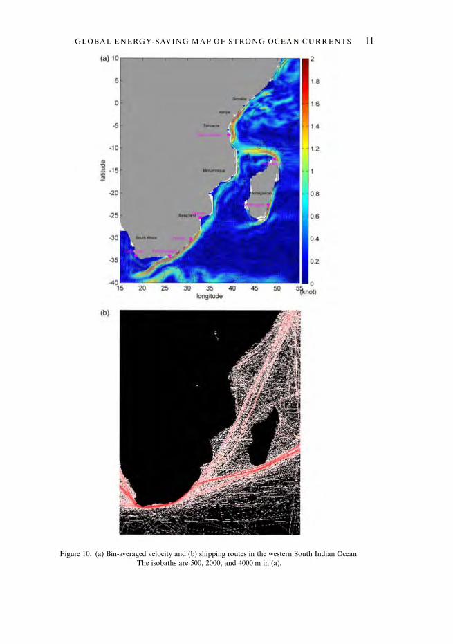
Figure 10. (a) Bin-averaged velocity and (b) shipping routes in the western South Indian Ocean.The isobaths are 500, 2000, and 4000 m in (a).

11GLOBAL ENERGY-SAVING MAP OF STRONG OCEAN CURRENTS

(a) 10 2

5 1 8

0 1 6

-5 1 4

-10 1 2

Ql

~ -15 .:> ~

-20 0.8

·25 0.6

0.4

02

0 20 25 30 35 40 45 50 5{\<not)

longitude

(b)

consume more fuel by taking the route which is against the strong adverse currents.Therefore, a better knowledge of the KC principal path and velocities can benefitoptimal ship routing and save ships’ operating costs. Chang et al. (2013b) suggestedthat the saving of transit time or the equivalent fuel consumption is more pronouncedin avoiding the adverse current on the return trip than following the Kuroshio on thenorthbound route.In the western equatorial Pacific, the North Equatorial Current (NEC) flows west-

ward toward the Philippine Islands near 10°N (Figure 8(a)). As the NEC approachesthe Philippine coast it splits into two branches, with the KC as its northward branchand the Mindanao Current (MC) as its southward branch. The current speed of thesouthward-flowing MC is larger than 2 knots along the east coast of MindanaoIsland. As the MC flows past the south of Mindanao, it splits into two branches.One branch flows eastward, and merges into the eastward-flowing North EquatorialCounter Current (NECC). The other branch moves westward, through the CelebesSea, and then flows rapidly through the Makassar Strait (Figure 8(a)). In theMakassar Strait, the southward currents are very strong (about 3 knots).The Makassar Strait and the east of Mindanao are common shipping routesbetween the Pacific and the Indian Ocean. Flows in the surrounding waters ofIndonesia and Philippines are very strong. Taking advantage of the strong currentsin this region will be a great benefit for all vessels to make optimal routing andreduce fuel consumption.In the south western Pacific Ocean, the southward-moving East Australian Current

(EAC) originates from the South Equatorial Current (SEC) (Godfrey et al., 1980). Asthe largest ocean current close to the eastern shores of Australia (Figure 9(a)), the EAChas a maximum speed of up to 7 knots in some of the shallow waters, but generally hasa speed of 2 knots. The mean velocity of EAC from 21 years of satellite sensor obser-vations reaches 1·6 knots. Figure 9(b) indicates that the routes of almost all north-bound ships in this region are running against the southward EAC. Thus a detailedand complete map of EAC (Figure 9(a)) is helpful for all types of ships.

6. STRONG CURRENTS IN THE INDIAN OCEAN. The Agulhas Current(AC) is the WBC of the south Indian Ocean, and is even suggested as the largestWBC in the oceans. It flows southward along the south eastern coast of Africa from27°S to 40°S, and has an estimated net transport of 100 Sv (1 Sv = 106 m3/s)(Bryden et al., 2003). There are two strong currents near the Madagascar Island(Figure 10(a)). Along the eastern coast of the island, a southward-flowing currentexists. On the north eastern corner of the island, a strong current flows westwardtoward Africa, and splits into two branches as it hits the coast. The northern branchflows northward, with a maximum speed of about 1·5 knots along the Tanzania-Kenya-Somalia coast. On the other hand, the southern branch joins the AC andflows southward. The AC gets stronger as it approaches the east coast of SouthAfrica, reaching a surface speed of 3–4 knots. In the Indian Ocean, piracy off thecoast of Somalia has been a threat to all types of vessels. Since 2005, IMO and theWorld Food Program (WFP) have expressed concern over the rise in acts of piracy(http://en.wikipedia.org/wiki/Piracy_in_Somalia). There were 127 and 151 attacks onvessels in 2010 and 2011, respectively. During 2013, the US Office of NavalIntelligence indicated that only nine ships had been attacked because of armed

12 YU-CHIA CHANG AND OTHERS

private security or significant naval presence on board ships. Thus, in the Somaliawaters, shipping routes are often far away from the shore (Figures 4 and 10(b)).

7. DISCUSSION. Weather routing of ocean-going shipping has been practiced formany years. During the last few decades there have been major advances in meteoro-logical analysis techniques and atmospheric modelling, which produce accurate globalforecasts of winds and waves for up to a week ahead, and to give some detail aboutlarge scale patterns for maybe another week beyond that. Based on this informationvessels can be routed to avoid severe storms or adverse sea state so as to minimisethe transit time and to evade significant risks to the vessel, crew and cargo. In thepast, current data was mostly extracted from ships’ logs, and these vast numbers ofobservations were compiled into pilot charts of monthly averages which serve as themain source of ocean current information for masters and other interested parties.These pilot charts only provide a rough estimate of the position and speed of oceancurrents, thus ocean currents traditionally were not taken into serious considerationfor optimum ship routing.The advent of satellite altimeters capable of measuring to a high degree of accuracy

the elevation of the sea surface has revolutionized the way ocean surface currents areobserved. Nowadays more and more operational ocean models (such as HYCOM,https://hycom.org/) have adopted real-time surface elevation and ocean current dataas the initial and boundary conditions of the model. However, incorporating themodel-produced real-time ocean current data into the ship routing decision processesis still at an early stage. Kobayashi et al. (2011) proposed a new weather routingmethod that accounts for ship manoeuvring motions, ocean current, wind andwaves through a time domain computer simulation to minimise fuel consumption.The target ship of Kobayashi et al. (2011) was a large container ship that traversesthe Pacific Ocean, and ocean current data over five-day averages and a 1° × 1° meshwere acquired from NOAA. The present study, by using 21 years of satellite-derivedgeostrophic currents data, provides a detailed (1/3° × 1/3°) and complete global mapof ocean surface currents. It is our hope that the climatology of ocean surfacecurrent patterns provided by our study can serve as a preliminary attempt towardsoptimum ship routing in the shipping industry. Although strong ocean currents suchas the WBCs in all oceans are largely in steady state and only change slowly over aperiod of days, the space-time variations of surface currents can still be substantial.In order to achieve an overall benefit in practice, detailed information on the space-time variations of ocean currents are needed in addition to the averaged globalocean currents provided by our study. There are a few internet sources on oceancurrents either from satellite remote sensing data (http://www.myocean.eu/web/69-myocean-interactive-catalogue.php), drifting buoys and HYCOM results (http://oceancurrents.rsmas.miami.edu/), or from a mixture of various in-situ observations and nu-merical modelling (http://oceanmotion.org/html/resources/oscar.htm), all can provideup-to-date ocean surface current information. Using the information of strongocean currents for ship routing can save fuel and reduce transit time to a certainextent by riding favourable currents and avoiding adverse currents. Slower vesselsare much more affected by currents, as the speed of the current is a much larger per-centage of the vessel speed. For a boat with a sailing speed of 6 knots and a distanceof 30 nm (spend 5 hours), riding favourable currents of 2–3 knots can save 25–33%

13GLOBAL ENERGY-SAVING MAP OF STRONG OCEAN CURRENTS

(spend 3·75, and 3·33 hours) on transit time and the equivalent fuel consumption.Avoiding adverse currents of 2–3 knots can save up to 33–50% (spend 7·5, and 10hours).Moore and Chang (1980) define Decision Support Systems (DSS) as extendible

systems capable of supporting data analysis and decision modelling, orientedtoward future planning and used at irregular and unplanned intervals. DSSs wereused for scheduling ocean-borne transportation and operations of a container terminalin earlier studies (Stott, 1981; Ronen, 1983; Christiansen et al., 2004; Murty et al.,2005). Existing ship routing DSS in the scheduled liner shipping industry are mainlyfocused on the inclusion of wind and wave data. The information of global ocean cur-rents provided by this work could be included in a future DSS for the optimisation ofship routes. A voyage between Wushih harbour in north eastern Taiwan and Daioyu(Sankahu) Island north east of Taiwan is exemplified to demonstrate the importanceof strong ocean currents in the optimisation of ship routing. The straight, most-directroute between these two locations has a distance of 102 nm (189 km) (red line inFigure 11), and the time it takes to complete this northbound voyage is 11·1 hoursat a ship speed of approximately 8 knots, with some speed gains from the favourable

Figure 11. Ship routing laid over bin-averaged strong currents betweenWushih harbor and Diaoyu(Senkahu) Islands. The red line represents the northbound straight route. The recommended routeof the return leg is in blue line which diverts from the adverse Kuroshio. See text for details.

14 YU-CHIA CHANG AND OTHERS

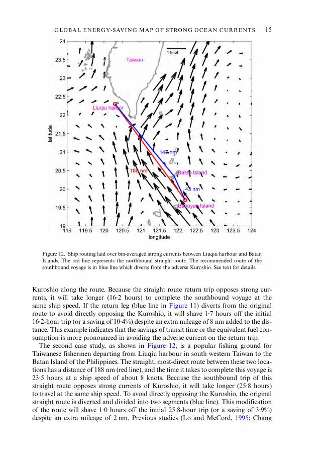
Kuroshio along the route. Because the straight route return trip opposes strong cur-rents, it will take longer (16·2 hours) to complete the southbound voyage at thesame ship speed. If the return leg (blue line in Figure 11) diverts from the originalroute to avoid directly opposing the Kuroshio, it will shave 1·7 hours off the initial16·2-hour trip (or a saving of 10·4%) despite an extra mileage of 8 nm added to the dis-tance. This example indicates that the savings of transit time or the equivalent fuel con-sumption is more pronounced in avoiding the adverse current on the return trip.The second case study, as shown in Figure 12, is a popular fishing ground for

Taiwanese fishermen departing from Liuqiu harbour in south western Taiwan to theBatan Island of the Philippines. The straight, most-direct route between these two loca-tions has a distance of 188 nm (red line), and the time it takes to complete this voyage is23·5 hours at a ship speed of about 8 knots. Because the southbound trip of thisstraight route opposes strong currents of Kuroshio, it will take longer (25·8 hours)to travel at the same ship speed. To avoid directly opposing the Kuroshio, the originalstraight route is diverted and divided into two segments (blue line). This modificationof the route will shave 1·0 hours off the initial 25·8-hour trip (or a saving of 3·9%)despite an extra mileage of 2 nm. Previous studies (Lo and McCord, 1995; Chang

Figure 12. Ship routing laid over bin-averaged strong currents between Liuqiu harbour and BatanIslands. The red line represents the northbound straight route. The recommended route of thesouthbound voyage is in blue line which diverts from the adverse Kuroshio. See text for details.

15GLOBAL ENERGY-SAVING MAP OF STRONG OCEAN CURRENTS

et al., 2013b) reported that ships can save 2–8% traveling time with sailing speedsaround 12–16 knots for the routes taking advantage of the KC and Gulf Stream.For fishing boats with a sailing speed of 8 knots, riding on KC can save about4–10% fuel. In the future, a better DSS in the scheduled liner shipping industrycould be developed taking the factors of currents, winds, waves, and other weather var-iations into consideration.Global fishing vessels are estimated to consume about 41 million tonnes of fuel per

annum (World Bank and FAO, 2009). This amount of fuel generates approximately130 million tonnes of CO2. Therefore having a detailed and correct map with globalstrong currents with statistics (Chu, 2008; 2009) is very important. Another importantcontribution of this study is to provide exact locations of strong currents in the world’sseas. In the future, locations, current speeds, and current directions of global strongflows could also be built into electronic chart systems for all navigators.

8. SUMMARY. Theoretically, riding strong currents with speeds of 2–3 knots oravoiding adverse currents can save 25–50% of fuel at a sailing speed of 6 knots.Thus knowledge of the WBC dominant path can be considered essential for all shiprouters. On the route of the KC region between Tokyo and Taipei (∼ 1100 nm),ships can save 2–6% fuel with sailing speeds of around 12 knots (Chang et al.,2013b). On the route of the Gulf Stream region (Lo and McCord, 1995), ships cansave 5–8% fuel with sailing speeds about 16 knots. The 2–8% fuel saving is significantfor shipping companies. On the other hand, the fuel savings are greater at lower sailingspeeds than at higher sailing speeds. On routes in the KC region, ships can save 4–10%fuel with sailing speeds of around 8 knots. For approximately 1·8 million small fishingvessels with lower ship speeds, making use of these strong currents wisely can save fuelsand reduce CO2 emissions significantly. The study makes a useful effort to introduce anovel approach, which is the use of remotely sensed ocean current data for the naviga-tion of ships. Analysing the AVISO satellite altimeter data is an important step towardsreal-time use for future electronic navigation.

ACKNOWLEDGEMENTS

This research was completed with grants from the Ministry of Science and Technology ofTaiwan, Republic of China (MOST 102-2611-M-110-010-MY3). Peter C. Chu was supportedby the Naval Oceanographic Office (N6230612PO00123). Ting-Peng Liang provides valuablesuggestions on Decision Support System. We are grateful for the comments from two anonym-ous reviewers.

REFERENCES

Ambe, D., Imawaki, S., Uchida, H., and Ichikawa, K. (2004). Estimating the Kuroshio axis south of Japanusing combination of satellite altimetry and drifting buoys, Journal of Oceanography, 60, 375–382.

Bryden, H. L., Beal, L.M., and Duncan, L.M. (2003). Structure and transport of the Agulhas Current andits temporal variability. Journal of Oceanography, 61, 479–492.

Chang, Y.-C., Tseng, R.-S., and Centurioni, L. R. (2010). Typhoon-induced strong surface flows in theTaiwan Strait and Pacific. Journal of Oceanography, 66, 175–182.

16 YU-CHIA CHANG AND OTHERS

Chang, Y.-C., Chen, G.-Y., Tseng, R.-S., Centurioni, L. R., and Chu, P. C. (2012). Observed near-surfacecurrents under high wind speeds. Journal of Geophysical Research, 117, C11026, doi:10.1029/2012JC007996.

Chang, Y.-C., Chen, G.-Y., Tseng, R.-S., Centurioni, L. R., and Chu, P. C. (2013a). Observed near-surfaceflows under all tropical cyclone intensity levels using drifters in the northwestern Pacific. Journal ofGeophysical Research, 118, 2367–2377.

Chang, Y.-C., Tseng, R.-S., Chen, G.-Y., Chu, P. C., and Shen, Y.-T. (2013b). Ship Routing Utilizing StrongOcean Currents. Journal of Navigation, 66, 825–835.

Christiansen, M., Fagerholt, K. and Ronen, D. (2004). Ship routing and Scheduling: status and perspectives.Transportation Science, 38(1), 1–18.

Chu, P. C. (2008). Probability distribution function of the upper equatorial Pacific current speeds.Geophysical Research Letters, 35, doi: 10.1029/2008GL033669.

Chu, P. C. (2009). Statistical characteristics of the global surface current speeds obtained from satellite altim-eter and scatterometer data. IEEE Journal of Selected Topics in Applied Earth Observations and RemoteSensing, 2 (1), 27–32.

Ducet, N., Le Traon, P.-Y., and Reverdin, G. (2000). Global high resolution mapping of ocean circulationfrom TOPEX/Poseidon and ERS-1 and -2. Journal of Geophysical Research, 105, 19477–19498.

FAO (2012). The state of world fisheries and Aquaculture 2012, Food and Agriculture Organization of theUnited Nations, Rome. ISBN 978-92-5-107225-7 (http://www.fao.org/docrep/016/i2727e/i2727e.pdf).

Godfrey, J. S., Cresswell, G. R., Golding, T. J., Pearce, A. F. and Boyd, R. (1980). The Separation of the EastAustralian Current. Journal of Physical Oceanography, 10, 430–440.

Halpern, B. S.,Walbridge, S., Selkoe, K. A., Kappel, C. V.,Micheli, F., Agrosa, C. D., Bruno, J. F., Casey, K. S.,Ebert, C., Fox, H. E., Fujita, R., Heinemann, D., Lenihan, H. S., Madin, E.M. P., Perry, M. T., Selig, E. R.,Spalding, M., Steneck, R., andWatson, R. (2008). AGlobalMap of Human Impact onMarine Ecosystems.Science, 319(5865), 948–952.

Hsueh, Y., Schultz, J. R., and Holland, W. R. (1997). The Kuroshio flow-through in the East China Sea: anumerical model. Progress in Oceanography, 39, 79–108.

International Maritime Organization, (2009a). Guidelines for voluntary use of the ship energy efficiency op-erational indicator (EEOI), IMO-MEPC.1/Circ.684, 17 August 2009 (http://www.imo.org/blast/blastDataHelper.asp?data_id=26531&filename=684.pdf).

International Maritime Organization, (2009b). Second IMO GHG Study 2009, IMO-MEPC 59/INF.10/Corr.1, April 2009 (http://www.imo.org/blast/blastDataHelper.asp?data_id=26046&filename=4-7.pdf).

International Maritime Organization, (2010). Reduction of GHG emissions from ships, IMO-MEPC 61/INF.22, 2 August 2010 (http://www.imo.org/OurWork/Environment/PollutionPrevention/AirPollution/Documents/INF-2.pdf).

International Maritime Organization, (2011). Assessment of IMOMandated energy efficiency measures forinternational shipping, IMO-MEPC 63/INF.2, 31 October 2011 (http://www.imo.org/MediaCentre/HotTopics/GHG/Documents/REPORT%20ASSESSMENT%20OF%20IMO%20MANDATED%20ENERGY%20EFFICIENCY%20MEASURES%20FOR%20INTERNATIONAL%20SHIPPING.pdf).

International Maritime Organization, (2012). 2012 Guidelines for the development of a ship energyefficiency management plan (SEEMP), IMO-MEPC 63/23, 2 March 2012 (http://www.imo.org/KnowledgeCentre/IndexofIMOResolutions/Documents/MEPC%20-%20Marine%20Environment%20Protection/213%2863%29.pdf).

Kobayashi, E., Asajima, T. and Sueyoshi, N. (2011). Advanced Navigation Route Optimization for anOceangoing Vessel. TransNav, the International Journal on Marine Navigation and Safety of SeaTransportation, 5, No. 3, 331–336.

Le Traon, P.-Y. and Dibarboure, G. (1999). Mesoscale mapping capabilities of multi-satellite altimeter mis-sions. Journal of Atmospheric of Oceanic Technology, 16, 1208–1223.

Le Traon, P.-Y., Dibarboure, G., and Ducet, N. (2001). Use of a High-Resoulution Model to Analyze theMapping Capabilities of Multiple-Altimeter Missions. Journal of Atmospheric of Oceanic Technology,18, 1277–1288.

Le Traon, P.-Y., F. Nadal, and Ducet, N. (1998). An improved mapping method of multisatellite altimeterdata. Journal of Atmospheric of Oceanic Technology, 15, 522–534.

Lo, H. K., and McCord, M. R. (1995). Adaptive ship routing through stochastic ocean currents: Generalformulations and empirical results. Transportation Research, A, 32, 547–561.

Moore, J. H. and Chang, M.G. (1980). Design of decision support systems. Data Base, 12, Nos. 1 and 2.Munk, W. H. (1950). On the wind-driven ocean circulation. Journal of Meteorology, 7, 79–93.

17GLOBAL ENERGY-SAVING MAP OF STRONG OCEAN CURRENTS

Murty, K.G., Liu, J., Wan, Y. and Linn, R. (2005). A decision support system for operations in a containerterminal. Decision Support Systems, 39, 309–332.

Pascual, A., Faugere, Y., Larnicol, G., and Le Traon, P-Y. (2006). Improved description of the ocean meso-scale variability by combining four satellite altimeters. Geophysical Research Letters, 33, L02611, doi:10.1029/2005GL024633.

Qiu, B. and Chen, S. (2006). Decadal variability in the large-scale sea surface height field of the south pacificocean: Observations and causes. Journal of Physical Oceanography, 36(9):1751,doi:10.1175/JPO2943.1.

Rio, M.-H., and Hernandez, F. (2004). A mean dynamic topography computed over the world ocean fromaltimetry, in situ measurements, and a geoid model. Journal of Geophysical Research, 109, C12032, doi:10.1029/2003JC002226.

Ronen, D. (1983). Cargo ships routing and scheduling: Survey of models and problems. European Journal ofOperational Research, 12, 119–126.

Silveira, I.C.A. da, de Miranda, L.B., and Brown, W.S. (1994). On the origins of the North Brazil Current.Journal of Geophysical Research., 99(22), 501–22, 512.

Stommel, H. (1948). The westward intensification of wind-driven ocean currents, Transactions of theAmerican Geophysical Union, 29, 202–206.

Stott, K. L., Jr. and Douglas, B.W. (1981). A model-based decision support system for planning and sched-uling ocean-borne transportation. Interfaces, 11:4, 1–10.

Wikipedia Website (2014). [Availableonlineathttp://en.wikipedia.org/wiki/File:Shipping_routes_red_black.png]

World Bank and FAO. (2009). The sunken billions. The economic justification for fisheries reform.Washington, DC, Agriculture and Rural Development Department, The World Bank. 100 pp.

Yamashiro, T., and Kawabe, M. (1996). Monitoring of position of the Kuroshio axis in the Tokara Straitusing sea level data. Journal of Oceanography, 52, pp. 675–687.

Yuan, D., Han, W. and Hu, D. (2006). Surface Kuroshio path in the Luzon Strait area derived from satelliteremote sensing data. Journal of Geophysical Research, 111, C11007, doi:10.1029/2005JC003412.

18 YU-CHIA CHANG AND OTHERS