Global Dynamics in a Search and Matching Model of the

Labor Market∗

Nika LazaryanFederal Reserve Bank of Richmond†

Thomas A. LubikFederal Reserve Bank of Richmond‡

October 2017

Working Paper No. 17-12

Abstract

We study global and local dynamics of a simple search and matching model ofthe labor market. We show that the model can be locally indeterminate or have noequilibrium at all, but only for parameterizations that are empirically implausible. Incontrast to the local results, we show that the model exhibits chaotic and periodicdynamics for reasonable parameter values both in backward and forward time. Incontrast to earlier work, we establish these results analytically without placing numericalrestrictions on the parameters.

JEL Classification: C62, C65, E24, J64

Key Words: Indeterminacy, Bifurcation, Chaos, Backward Map, Forward Map

∗The authors wish to thank Andreas Hornstein, Hassan Sedaghat and Alex Wolman for useful discussions.We would also like to thank participants at the 25th Annual Symposium of the Society for NonlinearDynamics and Econometrics in Paris for many comments. The views expressed in this paper are those ofthe authors and should not be interpreted as those of the Federal Reserve Bank of Richmond or the FederalReserve System.†

‡Research Department, P.O. Box 27622, Richmond, VA 23261. Email: nika.lazaryan@rich.frb.org Research Department, P.O. Box 27622, Richmond, VA 23261. Email: thomas.lubik@rich.frb.org.

DOI: https://doi.org/10.21144/wp17-121

1 Introduction

The search and matching model of the labor market has proved to be a convenient frame-

work for studying the joint behavior of unemployment and job vacancies. Much of the

qualitative and quantitative analysis in this framework relies on linear approximations and

local solutions of fundamentally nonlinear environments, as does most of the dynamic liter-

ature in macroeconomics. Yet, researchers have increasingly come to realize that the global

dynamics of such frameworks can have quite different implications than those derived from

local counterparts. In particular, nonlinear dynamics can be periodic or chaotic, which a

linear approach cannot capture. Moreover, a purely linear approach may rule out steady

state equilibria as unstable concluding explosive dynamics, and miss on cyclical equilibria

or stable dynamics elsewhere in the economic domain. Without a full characterization of

the nature of the processes that generate economic data, any conclusions drawn based on a

local approach might be misleading (see, for example, Wolman and Couper, 2003).

In this paper, we therefore study the global and local dynamics of the simple search

and matching model. Specifically, we add to the literature by showing analytically that the

model exhibits periodic and chaotic dynamics for a wide range of plausible parameterizations

that have been used in the quantitative literature. We employ analytic proofs that are

derived without placing numerical restrictions on the parameters. We are aided in this effort

by the specific structure of the search-and-matching framework, which can be reduced to a

recursive two-variable system. The model is thereby amenable to analytical characterization

of its local and global properties. The key dynamics arise from the model’s job-creation

condition, whereby we show that this is the case both in backward and forward time. For

the backward dynamics, we derive a mapping that can be easily analyzed after introducing

a variable change. This mapping ensures that the evolution of labor market dynamics is

both economically meaningful in the sense that trajectories of the model’s variables are

well defined, and that it is consistent with the model’s job-creation condition in terms of

uniqueness of the steady state. This differentiates our work from prior analysis of this

model, which uses a map that can have more than one steady state for certain parameter

values and may not always be defined on its domain.

Our paper contributes to the literature along two dimensions. First, the phenomenon

of chaotic dynamics in economic models is interesting on its own. However, most work has

focused on the Real Business Cycle (RBC) model or variants of the New Keynesian model,

whereby study of the global dynamics of the search-and-matching model is scant. Second,

2

our paper emphasizes the importance of considering global dynamics more broadly, espe-

cially since there is a growing awareness that reliance on local dynamics can be misleading.

For example, as is the case with our model, it can be shown that under certain conditions

the steady state may be a repeller, and it may therefore be tempting to conclude the model

exhibits explosive dynamics. We show that this is not always the case - the loss of stability

in the steady state coincides with emergence of cyclical behavior.

Our work builds on papers by Medio and Raines (2007) and Mendes and Mendes (2008).1

The former authors study backward dynamics in general economic models and provide the

general template for our analysis. Specifically, they develop general conditions under which

periodic and chaotic dynamics can arise in a wide class of economic models that can be

conveniently characterized by classes of mappings. Mendes and Mendes (2008) apply some

of these insights to a labor market framework that is similar to ours. They show that

the backward dynamics in the search and matching model can undergo a period-doubling

bifurcation that leads to chaos. However, this result is established under strict restrictions on

parameter values. Moreover, they show period doubling and existence of periodic points of

period 3 and 5 only numerically. Our work improves upon theirs by establishing existence of

periodic and chaotic solutions in the model analytically, which allows us to extend the range

of acceptable parameter values under which cycles and chaos can occur. From a technical

perspective, Mendes and Mendes (2008) use symbolic dynamics and inverse limit theory to

establish cycles and chaos going forward in time, when backward dynamics exhibits similar

behavior. Using the result established by Kennedy and Stockman (2008), we establish

chaotic and periodic solutions in forward time more generally, without imposing numerical

restrictions on parameter values.2

This paper is also close in spirit to recent contributions that analyze global dynamics

in Real Business Cycle models, such as Coury and Wen (2009), Growiec et al. (2015), and

Sorger (2016). In a RBC model with production externalities Coury and Wen (2009) show

that the unique steady state is surrounded by stable deterministic cycles, which implies

global indeterminacy that is not apparent from a local analysis. Their paper is similar to

1There is also earlier work by Bhattacharya and Bunzel (2003a,b), who study global dynamics in a searchand matching framework but impose parametric restrictions and only consider the social-planner solutionof the model. They establish the potential for n-period cycles in the model, but the modeling restrictionshave been criticized by Shimer (2004). Our paper can be seen as contribution that unifies and clarifies theseprevious results.

2Another paper that studies global dynamics in a search-and-matching setting in labor and capitalmarkets is Ernst and Semmler (2010). Their model has multiple steady states, one of which is a localattractor while another is saddle-path stable. Their analysis is fully numerical based on value-functioniteration, whereas we solve the nonlinear equilibrium conditions that emerge from the first-order conditions.

3

ours in that we also work in a two-equation environment that is amenable to straightfor-

ward, and intuitive, analytical and numerical analysis. As in our paper, they find that

indeterminacy is more pervasive than previously believed. Sorger (2016) extends this anal-

ysis to show that under standard monotonicity and convexity assumptions on technology

and preferences the basic RBC model can have periodic solutions of any period as well

as chaotic solutions. However, this does not arise for typical parameterizations that are

employed in the literature. In contrast, we show that in the search-and-matching frame-

work chaotic dynamics arise even under standard parameterization. Finally, Growiec at

al. (2015) show that in an extended version of the RBC model limit cycles can explain

the empirical evidence on substantial medium-to-long run, pro-cyclical swings in the labor

share in the U.S.

The paper is structured as follows. In the next section, we describe the simple search

and matching model of the labor market and derive the equilibrium conditions used in

the local and global analysis. We also discuss our calibration approach as it pertains to

the interpretation of our results. Section 3 presents the local determinacy properties of

the model. In Section 4, we turn to global dynamics. This section is the central part of

the paper, where we study the various global equilibria that arise in different regions of

the parameter space and contrast our findings with those from the local analysis. The

final section concludes. Relevant mathematical concepts and proofs are presented in the

Appendix.

2 A Simple Search and Matching Model of the Labor Market

We develop a simple version of the search and matching model of the labor market. The

model has become the workhorse framework for studying unemployment and vacancy dy-

namics and employment flows more generally, especially since Shimer’s (2005) seminal con-

tribution. The exposition below follows closely Krause and Lubik (2010), to which we refer

for further details.

2.1 The Model

We assume time is discrete and the model period is one quarter. A continuum of identical

firms employs workers who inelastically supply one unit of labor.3 Output y of a typical

3For expositional convenience, we present the problem of a representative firm only. We abstract fromindexing the individual variables.

4

firm is linear in employment n:

yt = Atnt, (1)

where At is an exogenous aggregate productivity process to be specified later.

Matching between workers and firms is captured by the function m(ut, vt) = muξtv1−ξt ,

with unemployment u, vacancies v, and parameters m > 0 and 0 < ξ < 1. m is the

match efficiency and measures the effectiveness of the matching process, while ξ is the

match elasticity. The matching function describes the number of newly formed employment

relationships that arise from the contacts between unemployed workers and firms seeking

to fill open positions. Unemployment is defined as:

ut = 1− nt, (2)

which is the measure of all potential workers in the economy who are not employed at the

beginning of the period and are thus available for job search activities.

We can write the law of motion for employment as follows:

nt = (1− ρ)[nt−1 +m(ut−1, vt−1)], (3)

where new hires add to the existing stock of workers. The end-of-the-period workforce is

subject to separation at the rate 0 < ρ < 1.4 We define q(θt) as the probability of filling

a vacancy, or the firm-matching rate, where θt = vt/ut is labor market tightness. In terms

of the matching function, we can write this as q(θt) = m(ut, vt)/vt = mθ−ξt . Similarly, the

job-finding rate is p(θt) = m(ut, vt)/ut = mθ1−ξt . An individual firm is atomistic in the

sense that it takes the aggregate matching rate q(θt) as given. The employment constraint

on the firm’s decision problem is therefore linear in vacancy postings:

nt = (1− ρ)[nt−1 + vt−1q(θt−1)]. (4)

Firms maximize profits, using the discount factor βt λtλ0 (to be determined below):

max{vt,nt}∞t=0

∞∑t=0

βtλtλ0

[Atnt − wtnt − κvt] + (5)

+∞∑t=0

βtλtλ0µt [(1− ρ)[nt−1 + vt−1q(θt−1)]− nt] .

Wages paid to the workers are w, while κ > 0 is a firm’s cost of posting a vacancy. µ is

the Lagrange-multiplier on the firm’s employment constraint. It can be interpreted as the

4Note that newly matched workers who are separated from their job within the period reenter the match-ing pool immediately.

5

marginal value of a filled position. Firms decide how many vacancies to post and how many

workers to hire. The first-order conditions are:

nt : µt = At − wt + β(1− ρ)λt+1

λtµt+1, (6)

vt : κ = β(1− ρ)λt+1

λtµt+1q(θt), (7)

which imply the job-creation condition (JCC):

κ

q(θt)= (1− ρ)β

(λt+1

λt

)[At − wt+1 +

κ

q(θt+1)

]. (8)

This optimality condition trades off expected hiring cost κ/q(θt) against the benefits of a

productive match. This consists of the output accruing to the firm net of wage payments

and the future savings on hiring costs when the current match is successful.

As is common in the literature, we assume the economy is populated by a representative

household. The household is composed of workers, who are either unemployed or employed.

If they are unemployed, they are compelled to search for a job, but they can draw unem-

ployment benefits b. Employed members of the household receive pay w, but share this with

the unemployed. They do not suffer disutility from working and supply a fixed number of

hours.5 Since the household’s only choice variable is consumption, and since there is no

mechanism to transfer resources intertemporally, the utility maximization problem is triv-

ial. Assuming constant relative risk aversion, this determines the marginal utility of wealth,

λt = C−σt , where C is consumption and σ−1 is the intertemporal elasticity of substitution.

In equilibrium, total income accruing to the household equals net output in the economy,

which is composed of production less real resources lost in the search process, Yt = yt−κvt.Since Ct = Yt, we can now derive the stochastic discount factor βt λtλ0 = βt

Y −σt

Y −σ0

.

Finally, we need to derive how wages are determined. We assume that wages are set

according to the Nash bargaining solution.6 As this is a lengthy, but standard, derivation,

we refer to Krause and Lubik (2010) for further exposition. The Nash-bargained wage is

thus:

wt = η (At + κθt) + (1− η)b. (9)

This equation can be substituted into the JCC to derive:

κ

mθξt = β(1− ρ)

Y σt

Y σt+1

[(1− η) (At − b)− ηκθt+1 +

κ

mθξt+1

]. (10)

This completes the description of the model.

5We thus assume income pooling between employed and unemployed households and abstract from po-tential incentive problems concerning labor market search. This allows us to treat the labor market separatefrom the consumption choice. See Merz (1995) and Andolfatto (1996) for a discussion of these issues.

6This is a standard assumption in the literature. Shimer (2005) provides further discussion.

6

2.2 Steady State

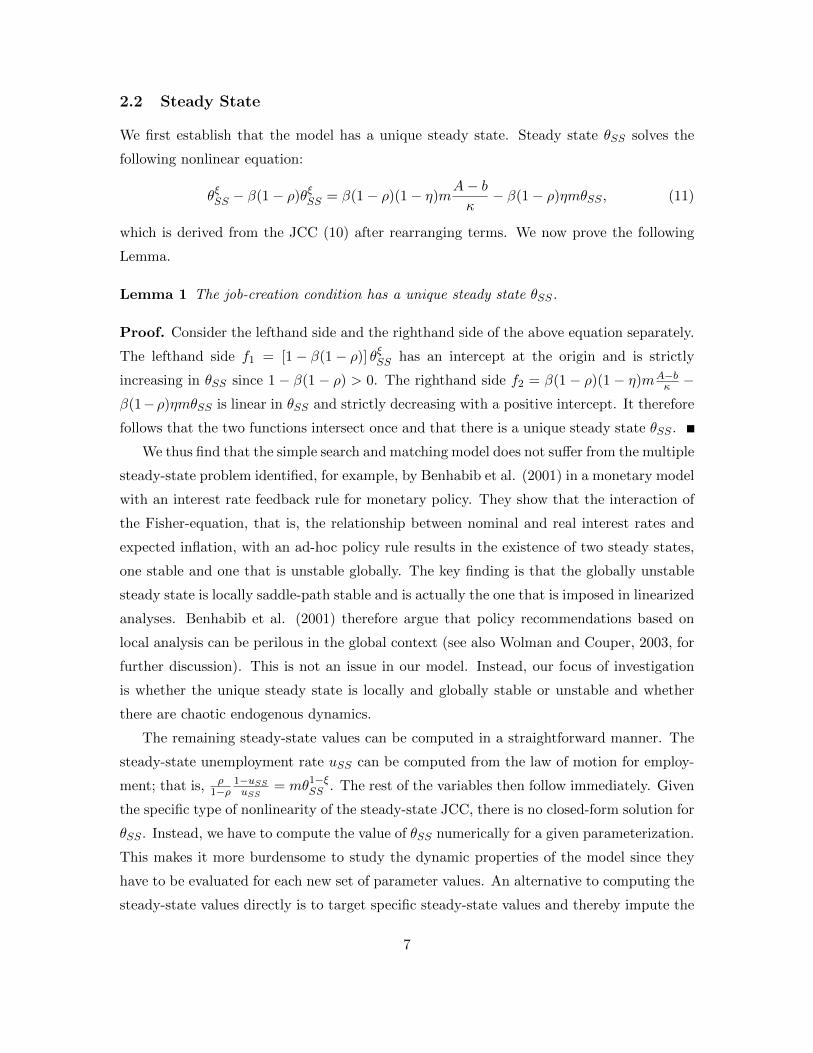
We first establish that the model has a unique steady state. Steady state θSS solves the

following nonlinear equation:

θξSS − β(1− ρ)θξSS = β(1− ρ)(1− η)mA− bκ− β(1− ρ)ηmθSS , (11)

which is derived from the JCC (10) after rearranging terms. We now prove the following

Lemma.

Lemma 1 The job-creation condition has a unique steady state θSS.

Proof. Consider the lefthand side and the righthand side of the above equation separately.

The lefthand side f1 = [1− β(1− ρ)] θξSS has an intercept at the origin and is strictly

increasing in θSS since 1− β(1− ρ) > 0. The righthand side f2 = β(1− ρ)(1− η)mA−bκ −

β(1−ρ)ηmθSS is linear in θSS and strictly decreasing with a positive intercept. It therefore

follows that the two functions intersect once and that there is a unique steady state θSS .

We thus find that the simple search and matching model does not suffer from the multiple

steady-state problem identified, for example, by Benhabib et al. (2001) in a monetary model

with an interest rate feedback rule for monetary policy. They show that the interaction of

the Fisher-equation, that is, the relationship between nominal and real interest rates and

expected inflation, with an ad-hoc policy rule results in the existence of two steady states,

one stable and one that is unstable globally. The key finding is that the globally unstable

steady state is locally saddle-path stable and is actually the one that is imposed in linearized

analyses. Benhabib et al. (2001) therefore argue that policy recommendations based on

local analysis can be perilous in the global context (see also Wolman and Couper, 2003, for

further discussion). This is not an issue in our model. Instead, our focus of investigation

is whether the unique steady state is locally and globally stable or unstable and whether

there are chaotic endogenous dynamics.

The remaining steady-state values can be computed in a straightforward manner. The

steady-state unemployment rate uSS can be computed from the law of motion for employ-

ment; that is, ρ1−ρ

1−uSSuSS

= mθ1−ξSS . The rest of the variables then follow immediately. Given

the specific type of nonlinearity of the steady-state JCC, there is no closed-form solution for

θSS . Instead, we have to compute the value of θSS numerically for a given parameterization.

This makes it more burdensome to study the dynamic properties of the model since they

have to be evaluated for each new set of parameter values. An alternative to computing the

steady-state values directly is to target specific steady-state values and thereby impute the

7

implied values of fixed parameters. If done judiciously, this would help avoid issues with

nonlinearity when solving for the steady state. We describe such an approach in the next

section when we discuss calibration.

2.3 Calibration

We now describe our choice for parameter values that we use in the numerical analysis

of the local and global properties. In our analysis, we assume, as in Shimer (2005), that

households are risk-neutral, that is, σ = 0. This simplifies derivation of analytical results

considerably and in fact makes it possible to obtain analytical results for global dynamics

(see also Bhattacharya and Bunzel, 2003a). We pursue two different strategies to assign

numerical values to the structural model parameters. One strategy sets the parameter values

directly. The advantage is that we can directly determine the impact of any parameter

changes on the behavior of the model. A drawback is that there is not much independent

information available for some of the parameters, and certain parameter choices can lead

to a priori implausible steady-state values. We can address this issue by imposing plausible

bounds on parameter values. Nevertheless, the steady state of the model is given by a

unique mapping from the structural parameters to the endogenous variables, as Lemma 1

shows. However, the mapping from the parameters to objects of interests may not admit

an analytical solution, of which one example is the computation of the steady state. Our

alternative strategy treats endogenous variables as parameters to be calibrated. In order

to obtain a specific target value, a parameter thus needs to be adjusted endogenously. The

advantage of this approach is that a judicious choice of setting steady-state values can allow

for analytical solutions.

We set the discount factor β = 0.99 and normalize the productivity level A = 1. The

separation rate ρ ∈ (0, 1). A typical value for quarterly data is ρ = 0.1, which is consistent

with the evidence reported in Shimer (2005). The bargaining parameter η ∈ (0, 1). The

vast majority of the literature assumes η = 0.5, as independent observations on its value are

not obvious to obtain. The match elasticity ξ ∈ (0, 1). In a well-known study, Petrongolo

and Pissarides (2001) advocate for values between 0.5 and 0.7. The plausibility of this

range is supported by the evidence in Lubik (2013). However, values outside this range can

be considered as well. The level parameter in the matching function m > 0 can be used

to scale, for instance, the unemployment rate, but it is otherwise left unrestricted in the

literature. However, we restrict this parameter to obey m ∈ (0, 1) based on the following

argument.

8

The job matching and job finding rates are defined as, respectively, q(θ) = mθ−ξ and

p(θ) = mθ1−ξ. These should properly be interpreted as the probabilities of a firm filling

a vacancy and a worker finding a job. It is a quirk of the discrete-time matching model

that mathematically these variables can take on values above one. Intuitively, at a low

enough frequency, everyone in the pool of searchers will transition out of unemployment at

least once, which translates into a job finding rate of above one. While this is conceptually

valid - the rate counts the number of new matches per searchers over a long enough period

- it violates the spirit of the search and matching model in that successful matching is

probabilistic. We note that this is not a problem for the continuous time version of the search

and matching model since q(θ) and p(θ) are instantaneous transition rates and thus are true

probabilities. In what follows, we therefore restrict these rates to lie on the unit interval (see

also Bhattacharya and Bunzel, 2003b, and Shimer, 2004). The following Lemma establishes

the necessary parametric restriction.

Lemma 2 The transition rates q(θ) and p(θ) are less than one if m < 1.

Proof. Define q(θ) = mθ−ξ and p(θ) = mθ1−ξ. q(θ) < 1 implies θ >(1m

)−1/ζ; p(θ) <

1 implies θ <(1m

)1/(1−ξ). For both transition rates to be less than one, this requires:(

1m

)−1/ζ< θ <

(1m

)1/(1−ξ). This is a nonempty interval for θ if m < 1.

As for the remaining parameters, benefits b ∈ (0, A) since they cannot exceed the

marginal product of the firm, in which case a firm could not offer any wage that would

induce an unemployed person to work. Given our normalization A = 1, this restricts b to

the unit interval. Typical values in the literature range from b = 0.4 (Shimer, 2005) to

b = 0.9 (Hagedorn and Manovskii, 2008). Vacancy posting cost κ > 0. It is a scale variable

that can be measured in terms of resource loss as a percentage of GDP. Typical values are

in the low percentage points when measured relative to output.

We also consider calibrating the steady-state unemployment rate uSS directly. Using

the law of motion for employment (3), we can then compute θSS =(

1m

ρ1−ρ

1−uSSuSS

)1/(1−ξ)without having to solve the nonlinear equation (11). Similarly, we can fix the job finding rate

pSS = p(θSS), which implies θSS = (pSS/m)1/(1−ξ). The JCC then delivers the following

restriction on the imputed parameter: A−bκ = η

1−ηθSS + 11−η

1−β(1−ρ)β(1−ρ)

θξSSm , from which we can

obtain either b, κ, or even η. We note that in this expression b and κ are not separately

identifiable. However, the term A−bκ scales various expressions, and we will discuss its

importance for global analysis further below. In terms of numerical values assigned to

the steady-state values, uSS can be chosen to correspond to observed sample means, which

9

typically is around 5%. An alternative approach is to target the observed employment rates,

which would imply an unemployment rate that is much higher, for instance, 25%. Both

approaches have been used in the literature, with different implications for the dynamic

behavior of the calibrated model.7

3 Local Dynamics

The local dynamics of the simple search and matching model have been studied by Krause

and Lubik (2010). We replicate their analysis here as a reference point for our study of

global dynamics. As discussed above we consider the case σ = 0 so that we can obtain an

analytical characterization. The job creation condition then becomes:

κ

mθξt = β(1− ρ)

[(1− η) (A− b)− ηκθt+1 +

κ

mθξt+1

]. (12)

We linearize this equation around the steady state, which results in:

θt = β(1− ρ)

(1− η

ξmθ1−ξSS

)θt+1, (13)

where θt = θt − θSS is the deviation from the steady state θSS .8 This is an autonomous

first-order linear difference equation in θ, the dynamic properties of which depend on the

coefficient β(1−ρ)[1− η

ξmθ1−ξSS

]. Since this is a forward-looking equation, a unique and de-

terminate equilibrium requires that the eigenvalue lies within the unit circle (see Blanchard

and Kahn, 1980). More formally, we establish the following Theorem.

Theorem 3 The equilibrium dynamics of the job-creation condition are locally unique if:

0 < p(θSS) <1 + β(1− ρ)

β(1− ρ)

ξ

η.

The equilibrium dynamics are locally indeterminate if:

1 > p(θSS) >1 + β(1− ρ)

β(1− ρ)

ξ

η

Proof. The equilibrium is locally unique if∣∣∣β(1− ρ)

(1− η

ξmθ1−ξSS

)∣∣∣ < 1. Consider the

boundaries in turn. Denote p(θSS) = mθ1−ξSS . β(1− ρ)(

1− ηξ p(θSS)

)< 1 implies p(θSS) >

7The idea is to capture both measured unemployment in terms of recipients of unemployment benefitsand potential job searchers that are only marginally attached to the labor force but are open to job search.Since we do not model labor force participation decisions, this is a shortcut to capturing effective labormarket search. This approach has been taken by Cooley and Quadrini (1999) and Trigari (2009).

8Log-linearizing this equation around the steady state would result in the same dynamic properties.

10

0 > − ξη1−β(1−ρ)β(1−ρ) , which is always true. Second, −1 < β(1 − ρ)

(1− η

ξ p(θSS))

implies

p(θSS) < ξη1+β(1−ρ)β(1−ρ) . Since 0 < p(θSS), this proves the first part of the theorem. The

equilibrium is indeterminate if∣∣∣β(1− ρ)

(1− η

ξmθ1−ξSS

)∣∣∣ > 1

The theorem is stated in terms of boundary conditions for the job finding rate p(θSS). We

find this useful for developing intuition as to the determinants of local and global dynamics

in the model. Moreover, as we pointed out above, the search and matching model is in

practice often calibrated in terms of target values for job matching and job finding rates.

Theorem 3 establishes that for a wide range of parameter values the dynamic equilibrium

is locally unique. Since the forward dynamics, obtained by iterating the linearized JCC

forward, are stable, the unique equilibrium is θt = 0, which puts labor market tightness

at its steady-state value as the only possible equilibrium. The steady state θSS is locally

unstable in this case. As time goes forward, the path for tightness will become unbounded

unless the economy is placed on the initial condition θ0 = θSS . Starting values in a small

neighborhood of the steady state will lead to explosive paths.

An alternative way to see this is by inverting the linearized JCC. This implies the

backward-looking representation θt+1 =[β(1− ρ)

(1− η

ξmθ1−ξSS

)]−1θt. The root of this

representation is the inverse of the root of the forward equation. Forward stability therefore

implies backward instability, and vice versa. Given the parametric restrictions established in

Theorem 3, the JCC would have explosive dynamics if expressed backward. Consequently,

the only solution to be consistent with local stability is θt = 0. One important insight is

that in the linear case the roots of the forward and the backward representation of the

difference equation in question are the inverse of each other. Local analysis can therefore

rely on either representation. This is, in general, not the case for global dynamics.

The equilibrium is locally indeterminate if the job-finding rate is high enough. In this

case, the JCC is a stable difference equation, one solution of which is, in fact:

θt+1 =

[β(1− ρ)

(1− η

ξmθ1−ξSS

)]−1θt. (14)

The steady state is therefore an attractor. All paths with starting values in a small neigh-

borhood around θSS converge to it. The different adjustment paths are indexed by their

starting values θi0, which correspond to the various dynamic equilibria. The threshold

for switching from a unique to an indeterminate local equilibrium is given by the term1+β(1−ρ)β(1−ρ)

ξη . High enough job-finding rates result in indeterminacy. Job-finding rates can

be high when the labor market is tight, that is, when there is a relatively high number of

vacancies compared to the pool of unemployed. In this case, equilibria can be self-fulfilling

11

because firms post additional vacancies even without supporting underlying fundamentals,

such as high productivity, because the high job-finding rates stimulate job search by the

unemployed and thereby validate the original vacancy posting.

Figure 1 depicts indeterminacy regions for various parameter combinations.9 The panels

with various parameter combinations show that for wide ranges of the parameter space, the

steady-state equilibrium is locally unique. Indeterminacy generally arises when the match

elasticity ξ is small. A special case is when ξ = η. This parameterization implements

the so-called Hosios-condition, under which the decentralized allocation is identical to the

social planner solution. In this case, p(θSS) < 1 < 1+β(1−ρ)β(1−ρ) , and local indeterminacy can

never arise, which is the main finding by Bhattacharya and Bunzel (2003a,b). In the lower

righthand panel, the Hosios-condition can be represented by the 45-degree line where η = ξ.

The indeterminacy region lies in the upper lefthand corner where the bargaining parameter

η is high and ξ small, which is consistent with Theorem 3.

However, the Hosios-condition is empirically violated as the literature has amply demon-

strated, and we do not regard this as a likely parameterization.10 The threshold is tight-

ened as the term ξη becomes smaller. Low values of the match elasticity and high values

for the bargaining share are therefore more likely to imply indeterminacy. For instance, for

β = 0.99, ρ = 0.1, ξ = 0.4, and η = 0.9, the threshold coefficient is 0.94. den Haan et al.

(2000) report an estimate for p(θ) of 0.45. Although this is far away from the threshold, we

would nevertheless regard the possibility of local indeterminacy as more than a curiosity.

4 Global Dynamics

We now turn to an analysis of the global dynamics. We first provide some general insights

into the properties of the nonlinear search and matching model and set up the map that

we use to study global equilibria. We start with the stability analysis of the steady state

and focus on the bifurcation that occurs when the dynamics switch from stable to unstable

in backward time. We show that this switch corresponds to cyclical behavior in the model

and establish the presence of chaotic dynamics in backward and forward time. Finally, we

explicitly link the bifurcation to the structural parameters of the economic model.

9The figure also shows regions where the equilibrium does not exist. But for the purposes of this paperwe rule these out on account of Lemma 2.

10See Lubik (2013) and the references cited therein.

12

4.1 Preliminaries

We analyze the benchmark case of an economy with risk-neutral agents as described above.

The dynamics are governed by the job-creation condition, which we replicate here for con-

venience:κ

mθξt = β(1− ρ)

[(1− η) (A− b)− ηκθt+1 +

κ

mθξt+1

]. (15)

This is an autonomous first-order nonlinear difference equation in θ. It describes the evo-

lution of labor market tightness θt and can be solved independently from the rest of the

model. As in the analysis of the local dynamics, this allows us to study the evolution of θt

in isolation.11 We rewrite the JCC by isolating terms in θt+1 on the lefthand side:

β(1− ρ)θξt+1 − β(1− ρ)mηθt+1 = θξt − β(1− ρ)(1− η)mA− bκ

. (16)

In coefficient form, we have:

aθξt+1 − cθt+1 = θξt − d, (17)

where:

0 < a = β(1− ρ) < 1,

0 < c = β(1− ρ)mη < 1,

0 < d = β(1− ρ)(1− η)mA− bκ

.

Equation (17) is in implicit form. The forward map is not invertible; that is, we cannot

explicitly relate θt+1 to θt. In other words, the forward dynamics are captured by a corre-

spondence. In this case, it is therefore much more convenient to study the global properties

using the backward dynamics.12 We then use the results in Kennedy and Stockman (2008)

to relate the backward dynamics to those in forward time.

In the previous literature, for example Mendes and Mendes (2008) and Bhattacharya

and Bunzel (2003 a,b), the backward dynamics are defined via the map g (θ) by rearranging

(17) to isolate θt:

θt =(aθξt+1 − cθt+1 + d

)1/ξ= g (θt+1) . (18)

11Under risk aversion, the dynamics depend on the time path of output yt. Output is a function ofemployment nt, which evolves based on the law of motion (3). Since this feeds back onto the JCC viathe definition of θt = vt/ut, it results in an interconnected two-equation system that cannot be solvedanalytically.

12The relationship between the backward and forward dynamics of nonlinear systems is an area of activeresearch (see, for example, Kennedy and Stockman (2008) and references thereof). This distinction isimmaterial for the study of linear systems since they are always invertible in this sense. That is, theproperties of the forward dynamics are the ‘inverse’ of the properties of the backward map. If, on the otherhand, one of the dynamic maps is a correspondence, this equivalence fails.

13

However, the choice of the map g is problematic, since it can produce results that are

inconsistent with the logic of the JCC. We show in Appendix A.2 that, for plausible values

of the parameter ξ, the map g can have multiple positive steady states, whereas the positive

steady state θSS in JCC is unique (see Lemma 1). To avoid this inconsistency, we therefore

introduce a change of variables such that for θt ≥ 0:

zt = θξt . (19)

This allows us to rewrite the equation in (17) as the following backward recurrence relation:

zt = azt+1 − cz1/ξt+1 + d = f(zt+1), (20)

where the coefficients are defined as above. Backward solutions of (17) and (20) are well-

defined for any ξ ∈ (0, 1), as long as zt and θt are non-negative. The solutions of (17) in

terms of the original variable can be obtained by using θt = z1/ξt . The model in the form

of (20) thus provides us with a more convenient and consistent means for studying the

backward dynamics of the model.

4.2 Stability Properties

We now study the dynamics of the backward map zt = f (zt+1). We first establish the

properties of the function f . We then study the stability properties of the steady state,

where we distinguish between two broad areas of dynamics in the backward map, namely

stable and unstable. The backward dynamics are governed by the properties of the map:

f(z) = az − cz1/ξ + d, (21)

where f(0) = d > 0 defines the intercept. The first derivative of f is given by:

f ′ (z) = a−(c

ξz

) 1−ξξ

, (22)

and the map f has a global maximum at:(aξ

c

) ξ1−ξ

:= zmax. (23)

Given that f is increasing on [0, zmax) and decreasing on (zmax,∞), the map f is a Type-

B map as defined in the Appendix A.3. The point z0 > 0 is the unique positive intersection

point such that f(z0) = az0− cz1/ξ0 + d = 0.13 Note that the coefficients are independent of

13It is straightforward to show that z0 is unique over [0,∞). Since f(0) = d > 0 and f is increasing on[0, zmax), then f(zmax) > 0. Given that f is decreasing on [zmax,∞), the intersection point z0 such thatf(z0) = 0 is unique. Note that the point z0 corresponds to the point q in Appendix A.3.

14

the match elasticity ξ, which therefore only determines the shape of the mapping but not

its location in (θt+1, θt)-space. Furthermore, the term A−bκ scales the intercept d but does

not affect other coefficients.

We can express the maximum of f in terms of the structural parameters of the model:

zmax =(aξc

) ξ1−ξ

=(

ξmη

) ξ1−ξ

. The maximum only depends on three parameters, which

reduce to two under the Hosios-condition ξ = η. In this special case, zmax > 1 since m < 1.

In the general case, zmax can be less than one if m > ξη . Notably, the location of the

maximal point does not depend on other parameters, chiefly the scale term A−bκ . In the

next step, we establish that the equation in (20) has a unique positive steady state. It is

straightforward to see that θSS = (zSS)1/ξ is the same as established in Lemma 1; that is,

θSS = (f (zSS))1/ξ.

Lemma 4 Equation (20) has a unique positive steady state zSS.

Proof. The steady state(s) of (20) must be the fixed point(s) of the map f in (21). The

fixed point(s) z of f must satisfy the equation

az − cz1/ξ + d = z.

To show that such a point z exists, we define a function φ(z) = (1− a)z + cz1/ξ − d. Since

φ(0) = −d < 0 and φ(

d1−a

)= c

(d

1−a

)1/ξ> 0, there exists a point z ∈

(0, d

1−a

)such that

φ(z) = 0. To show that z is unique, we note that the derivative φ′(z) = (1−a) + cξz

1−ξξ > 0

for z > 0. Therefore, φ is increasing on (0,∞), and hence its zero is unique. It follows

that z = zSS is the unique positive fixed point of the map f and the equation in (20) has a

unique positive steady state.

We now analyze the stability properties of the steady state. These properties are

determined around the thresholds ±1 and are given by the first derivative f ′ (zSS). If

|f ′ (zSS)| < 1, the steady state zSS is stable in its backward dynamics and unstable other-

wise. At |f ′ (zSS)| = 1 a bifurcation occurs, and the dynamics switch from stable to unsta-

ble. Clearly, the stability properties of zSS translate directly to that of θSS . |f ′ (zSS)| < 1

if and only if:

− 1 < a−(c

ξzSS

) 1−ξξ

< 1, (24)

or, alternatively:

a− 1 <

(c

ξzSS

) 1−ξξ

< 1 + a. (25)

15

Since the value of the parameter a is less than one, the first inequality above holds trivially,

given Lemma 4 and the restrictions on the parameters. This also means that whenever

f ′ (zSS) is positive, it is less than one. In other words, if zSS ≤ zmax, then zSS is stable.

Since a bifurcation cannot occur in this region of the map, we focus our attention on the

other case, namely f ′ (zSS) > −1. In the case when zSS > zmax, f ′ (zSS) is negative, and

the steady state zSS may or may not be stable. Since f ′ (zSS) > −1 implies that:

c

ξ(zSS)

1−ξξ < 1 + a, (26)

then zSS is stable if (26) holds; it is unstable otherwise. For reference, we collect these

results in Table 1.

We can also express these conditions in terms of the underlying structural parameters

of the model. The stability condition (26) can be written in terms of θSS as follows:

θSS <1 + β(1− ρ)

β(1− ρ)

ξ

mη. (27)

This is the counterpart to the case identified for local dynamics under indeterminacy, which

required a high enough job-finding rate p(θSS) or a high steady-state value θSS . The loss

of stability of θSS translates into stable adjustment dynamics for the forward map. The

solution to the model is such that starting from an initial value in a close neighborhood of

the steady state, the economy will converge nonmonotonically (since f ′ (zSS) < 0) to the

steady state, which is an attractor in the forward dynamics. The law of motion is given by

the correspondence (17).

We note that the conditions in (26) and, equivalently, in (27) are in implicit form since

zSS and θSS are functions of the composite parameters a, c, d, and ξ, and ultimately the

structural parameters; at the same time, the analytical expression for zSS cannot always be

obtained explicitly. We find it therefore convenient to express the threshold conditions in

terms of endogenous variables for ease of economic interpretation. In that sense, condition

(27) is an outcome of a stable equilibrium, in which the steady-state labor market tightness

is less than the given threshold. For the benchmark case ξ = 0.5, we can solve directly for

zSS and express the equation (29) and (27) in terms of model parameters only. We will

present results and discuss the benchmark case in the next subsection. We now turn to the

main section of the paper and an analysis of its key result.

16

4.3 Periodic and Chaotic Solutions

We establish in this section that the transition from stable and unstable dynamics at

f ′ (zSS) = −1 in backwards time corresponds with another type of a bifurcation, namely

the emergence of a sequence of cycles of doubling periods. That is, as the steady-state zSS

loses its stability and goes through this bifurcation, a new attractor emerges with double

the period of the steady state (i.e. a 2-cycle). The model’s solution oscillates between these

values but in a nonexplosive manner. As the value of the bifurcation parameter changes,

new attractors continue to appear of double the period of the previous ones. This even-

tually leads to bounded aperiodic and chaotic fluctuations in the dynamics of the model.

We first establish this result analytically in terms of the composite coefficients of the map

defined in the section on preliminaries above. We choose d as the bifurcation parameter,

since it scales in A−bκ . Whereas the parameters in the coefficients a and c are comparatively

tightly restricted, the parameters in this scale coefficient are less economically restricted as

discussed in the calibration section.

The change in stability of zSS occurs at f ′ (zSS) = −1, or:

c

ξ(zSS)

1−ξξ = 1 + a. (28)

We can rewrite (28) in terms of d as follows. At the steady state, we have f(zSS) =

azSS − cz1/ξSS + d = zSS , or a− c (zSS)1−ξξ + d

zSS= 1. Hence, c (zSS)

1−ξξ = a− 1 + d

zSS. We

can plug this expression this into (28) and find an alternative and equivalent condition to

(28):d

zSS= ξ(1 + a) + (1− a), or: d = µzSS , (29)

where µ = ξ(1 + a) + 1 − a. When d < µzSS , −1 < f ′(zSS) < 0; when d > µzSS ,

f ′(zSS) < −1. In addition, note that if ξ ≥ 0.5, µ ≥ 1 + 0.5(1 − a) > 1, since a < 1. We

can now establish the period doubling.14

Theorem 5 The point d∗ = µz∗SS is a bifurcation point for period doubling. Passing of d

through the bifurcation threshold corresponds with emergence of cycles of period 2, 4, 8, etc.

Proof. It is relatively straightforward to check the conditions required for period doubling

bifurcations given in Elaydi (2007) and summarized in Appendix A.1. For fixed values of

14The condition in (29) is expressed in implicit form since zSS depends on d, as well as a, c, and ξ. Weshow explicit analytical results in terms of model parameters only for the benchmark case ξ = 0.5 in thenext subsection.

17

a, c, ξ, the parameterized map is:

fd(z, d) = az − cz1/ξ + d.

It is easy to verify that the parameterized map fd(zSS) = zSS for d > 0, i.e., fd has a unique

positive fixed point zSS for all positive values of d. At the bifurcation point d∗ = µz∗SS ,∂fd∂zSS

(zSS) = −1. Finally, ∂2f2

∂d∂zSS(d∗, z∗SS) cannot be zero, where f2d is the composition of

the map f with itself, i.e., f2d (d, zSS) = fd(fd(d, zSS)). We have:

f2(d, z) = a(az − cz1/ξ + d)− c(az − cz1/ξ + d)1/ξ + d,

and:∂2fd∂z∂d

= − cξ

1− ξξ

(az − cz1/ξ + d)1−2ξξ (a− c

ξz

1−ξξ ) 6= 0,

for zmax < zSS < z0, which is our domain of analysis.

We illustrate this result by means of a simple example. Figure 2 demonstrates the period

doubling numerically. For fixed ξ = 0.5, a = 0.891 and c = 0.4 and a range of parameter

values of d > 0, we generate 500 iterates of the map f and plot the last 200 against d.

For low values of d, the iterates converge to a single steady state. Around d = 2.5, we see

emergence of a 2-cycle. Four cycles appear as d passes through 3.7, and one can also discern

the emergence of an 8-cycle past 4. For higher values of d, the shaded region of the diagram

shows aperiodic oscillations and is referred to as a chaotic region. A little past d = 5, we

can also discern a stable 3-cycle. This parameterization is only one example of emergence

of periodic doubling and chaos. These values are, however, economically plausible, as

a = 0.891 is obtained by setting the discount rate β = 0.99 and the job separation rate

ρ = 0.1. Under the Hosios-condition η = ξ = 0.5, the value of c = 0.4 implies that m is

around 0.9. For values of d between 5 and 5.5, the implied steady-state unemployment rate

uSS ranges between 0.167 and 0.174, which is well within economically plausible bounds.

Appendix A.3 presents additional sufficient and general conditions for existence of peri-

odic and chaotic solutions in Type-B maps. The results of Theorems 20, 21, and Corollary

22 therefore apply since our map f is of this type. We refer to the Appendix for a detailed

discussion and further proofs. In what follows, we interpret some of the conditions stated

in these theorems. First, Theorems 20 and 21 require that f(zmax) = z0 where z0 > zmax

is the preimage of 0, i.e., f(z0) = 0. However, in most cases, we cannot solve for z0 analyti-

cally. An alternative way of formulating this requirement is the following: for f(zmax) = z0,

it is necessary that the second iterate of zmax maps to zero, i.e., f2(zmax) = 0. Since

18

f(zmax) = a(aξc

) ξ1−ξ − c

(aξc

) 11−ξ

+ d, the condition f2(zmax) = 0 implies:

f2(zmax) = a2(aξ

c

) ξ1−ξ− ac

(aξ

c

) 11−ξ

+ ad− c

[a

(aξ

c

) ξ1−ξ− c

(aξ

c

) 11−ξ

+ d

] 1ξ

+ d = 0

(30)

The equation in (30) is in implicit form and defines a surface in a four-dimensional coefficient

space for a, d, c, ξ. For any fixed values of two of these parameters, one can plot implicit

curves in two dimensions to show parameter ranges that satisfy this condition. Figure 3

shows the plot of a family of such curves that also satisfy d < zmax (see Theorem 21) for

ranges of parameters when a is set at 0.891 and 0 < c < 1.

Denoting z+ as the right preimage of zmax, i.e., z+ > zmax is a point such that f(z+) =

zmax, then the case d > zmax and f(d) ≥ z+ in Theorem 21 (b) implies that f2(d) ≤zmax (since, again, we cannot always solve for z+ analytically). This corresponds with the

inequality:

a(ad− cd1/ξ + d)− c(ad− cd1/ξ + d

)1/ξ+ d ≤

(aξ

c

) ξ1−ξ

. (31)

The family of curves that satisfy (30) and the above inequality are presented graphically in

Figure 4 for ranges of parameters a = 0.891 and 0 < c < 1. Finally, the condition f(d) = z0

exactly pins down the three cycle {. . . , 0, d, z0, 0, d, z0, . . . }, as 0 → d → f(d) = z0 → 0.

This condition can be rewritten as f2(d) = 0, or:

a(ad− cd1/ξ + d)− c(ad− cd1/ξ + d

)1/ξ+ d = 0, (32)

as depicted in Figure 5.

In summary, Figures 3 - 5 give an idea for which parameterizations periodic and chaotic

dynamics can arise in the nonlinear model. Previously, Mendes and Mendes (2008) have

established chaos for ξ = 0.2. This is consistent with our finding that conditions in (30)

and d < zmax, as well as (32), imply low values of the match elasticity ξ, e.g. as in Figure 5.

However, empirical estimates of the parameter ξ in the literature are considerably higher.

Petrongolo and Pissarides (2001) find a value ξ of 0.7, while Hall and Schulhofer-Wohl (2015)

report estimates that range between 0.28 and 0.7 from a wide variety of studies, data, and

empirical approaches. In addition, and in contrast to the earlier literature on nonlinear

dynamics in the search and matching model, we find that the conditions in (30) and (31)

19

yield values of ξ that are consistent with these empirical estimates. We can summarize

these results in the following theorem. They are also collected in Table 1.

Theorem 6 For certain parametrization, the map f is chaotic, i.e. the equation in (20)

has chaotic as well as coexisting periodic equilibria of multiple periods. In particular,

(i) If (30) holds and zmax > d, then the equation in (20) has periodic equilibria of every

period p ≥ 3, as well as aperiodic and chaotic solutions.

(ii) If (30) and (31) hold and zmax < d, then the equation in (20) has periodic equilibria

of every period p ≥ 5, as well as aperiodic and chaotic solutions.

(iii) If (32) holds, then the equation in (20) has a 3-cycle.

As a final step, we relate the equilibria in backward time to those of their forward repre-

sentation. Translating cycles from backward to forward time (and vice-versa) is straightfor-

ward. Kennedy and Stockman (2008) show that equilibria in forward dynamics are chaotic

if and only if they are chaotic in backward time. This gives us our last theorem, which

comes as a consequence of Corollary 22 and Theorem 18 of the Appendix.

Theorem 7 Under certain parameterization, the equations in (20) and (17) have periodic

as well as chaotic equilibria going both forward and backward in time.

4.3.1 A Simple Illustration for a Benchmark Parameterization

We can derive analytic conditions for the existence of periodic and chaotic equilibria for the

special case when the match elasticity ξ = 0.5. This parameterization, which is empirically

plausible as discussed above, implies that the map f becomes the quadratic:

f(z) = az − cz2 + d. (33)

We can therefore explicitly solve for zSS , z0, and z+ as zSS = 12c

((1− a) +

√(1− a)2 + 4cd

),

z0 = 12c

(a+√a2 + 4cd

)and z+ = 1

2c

(a+√a2 + 4cd− 2a

). The critical value for period

doubling bifurcation d∗ = µzSS then corresponds to:

d∗ =1

2c

(1 +

1− a2

)((1− a) +

√(1− a)2 + 4cd∗

),

where the coefficients a and c are defined above. These curves are plotted in Figure 6 for

the same parameterization as discussed before. Over the admissible region 0 < c < 1, there

20

is a wide range of parameter combinations where chaotic behavior can occur. We will dig

deeper into the parameter regions that can imply periodic behavior in the next section.

We also want to highlight on additional case under this benchmark parameterization.

Whereas in Section 4.3 we provide sufficient conditions, these are not the only instances

where chaotic equilibria occur. For the quadratic case ξ = 0.5, it is also straightforward

to pin down the values of parameters a, c, d that establishe qualitative (or topological)

equivalence of the dynamic behavior of the iterates of the map f to those of the logistic

map r(µ) = µr(1 − r). The logistic map is a canonical example for demonstrating chaos

in one-dimensional maps, as, for example, in Elaydi (2007). Using the benchmark case, we

can solve for period-3 points of the map f numerically. Specifically, we solve for the fixed

points of the composite map f3 that are different from zSS . The parameter values where

such points are found are given in Figure 7 for the same ranges as before.

4.4 Chaos Regions for Structural Parameters

In this final section, we provide further insight into the economic determinants of the range

of equilibria by expressing them in terms of the structural parameters of the underlying

model. This is not quite straightforward since the search-and-matching model is richly

parameterized in the sense that the equilibrium and the dynamic behavior of one endogenous

variable, namely labor market tightness θ, is determined by eight parameters in the JCC. In

order to identify the relevant regions where chaos can occur, we therefore have to judiciously

condition on specific parameters values. Recall that the location of zmax =(

1mξη

) ξ1−ξ

is

determined by three parameters only. Furthermore, we keep the separation rate ρ and the

discount factor β fixed for the purposes of this analysis. We therefore find it convenient

to analyze the equilibria in terms of the other model parameters that affect the type of

equilibria and the shape of the map. This leaves the scale term A−bκ as the crucial coefficient

to analyze, whereby we normalize A = 1 without loss of generality. It can be ascertained

immediately that A−bκ shifts the map f (z) vertically, thereby changing the location of the

steady state zSS and the intercept z0 with the zero line. The shape of the map, however, is

unaffected.

Similar to the analysis of the local dynamics, we find it convenient to describe the

analytical properties of the map in terms of the steady-state values of endogenous vari-

ables. Specifically, we consider the steady-state unemployment rate uSS as a calibra-

tion target. Since θSS = z1/ξSS , we can then back out the implied labor market tightness

θSS =(

1m

ρ1−ρ

1−uSSuSS

)1/(1−ξ)from the law of motion for employment. However, we note that

21

the steady state θSS and therefore uSS are themselves functions of all of the structural pa-

rameters of the model. Given the JCC, this strategy then restricts the parameterization of

either b or κ based on the relationship A−bκ = η

1−ηθSS + 11−η

1−β(1−ρ)β(1−ρ)

θξSSm . It thus leaves one

remaining parameter for which we can do comparative static analysis. Intuitively, this ap-

proach targets a specific unemployment rate by setting, for instance, benefits b at a specific

level. Changing of b (or κ) necessarily changes the steady state uSS . Instead of discussing

the effects of changes in this parameter on the implied uSS , this reparameterization allows

us a more direct and economically intuitive consideration.

We now establish the following Lemma, which describes the regions of the structural

parameter space for which the first derivative of the map f is negative. We concentrate on

this case since it admits a bifurcation.

Lemma 8 For zmax < zSS < z0, f ′ (zSS) < 0. We distinguish three different regions of the

parameter space:

(i) 0 > f ′ (zSS) > −1:1

1 + β−1+(1−ρ)ρ

ξη

< uSS <1

1 + 1−ρρ

ξη

(ii) f ′ (zSS) = −1:

uSS =1

1 + β−1+(1−ρ)ρ

ξη

(iii) −1 > f ′ (zSS):

uSS <1

1 + β−1+(1−ρ)ρ

ξη

If the parameterization is such that condition (ii) holds, that is, if the endogenous

unemployment rate is equal to the threshold[1 + β−1+(1−ρ)

ρξη

]−1, then the equilibrium

undergoes a bifurcation. We can depict this scenario in terms of the structural parameters of

the model. This is presented in Figure 8. These graphs are created for ranges of composite

parameter values where chaos is observed. For a given point in the shaded region (for

instance m and u), there exist parameter values a, c, d, and ξ = 0.5, which result in chaotic

behavior in the model.15 We observe that chaos is prevalent in the nonlinear model for

economically plausible parameter values. Generally, we observe chaos for values of the

match efficiency parameter m above 0.5, which is consistent with empirical estimates. At

15Except for the case shown in m-ρ space of Figure 8, a is fixed at 0.891, which is obtained by settingβ = 0.99 and ρ = 0.1. We also impose the Hosios-condition that sets ξ = η.

22

the same time, chaotic behavior requires a high bargaining parameter η, a comparatively low

job matching rate q, and is consistent with a moderately high steady-state unemployment

rate u. On the other hand, combinations of the separation rate ρ and m that imply chaos

are in the plausible range for the former but not the latter.

It is instructive to contrast these findings to the results on local dynamics as described

in Section 3 and depicted in Figure 1. While we cannot talk about chaotic and periodic

behavior locally, one conclusion we can draw from analysis of the local dynamics is that

for a wide region of the parameter space the search-and-matching model exhibits locally

unique dynamics. It is only in extreme regions of the parameter space that we observe

explosive or excessively stable behavior, or in the language of local analysis nonexistence or

indeterminacy, respectively. In contrast, the possibility of periodic and chaotic dynamics is

pervasive in the sense that we can obtain such equilibria for an economically plausible and

reasonably large region of the parameter space.

5 Conclusion

This paper demonstrates that periodic and chaotic dynamics are an economically plausi-

ble feature of the simple search-and-matching model of the labor market. This stands in

contrast with findings from the literature on local dynamics that the model exhibits locally

unique and stable equilibria over the wide range of the parameter space. In contrast to

previous literature on global dynamics in this class of models, we are able to characterize

analytically a larger set of regions implying chaotic dynamics. Specifically, we show exis-

tence of chaos for calibrations that have been used in the literature. Moreover, we do so by

utilizing some recent results from the literature on chaotic equilibria.

Our paper is purely theoretical in nature, albeit with a focus on economically plausible

outcomes. What remains to be seen, however, is the extent to which the fully nonlinear

model with parameters that fall into the chaotic region is an actual data-generating process.

That is, do actual labor market time series, such as the unemployment rate and vacancies,

exhibit behavior of the type that are consistent with, say, periodic equilibria? For instance,

Figure 9 depicts time paths of labor market tightness with periodic and chaotic behavior

generated under different values of the match elasticity ξ. At first pass, this seems unlikely

since we do not typically observe such oscillating behavior in the data. This would, of course,

have to be established more formally. A second issue is the degree to which local theoretical

models or linear empirical methods fail in describing such global dynamics. Research in this

area is still sparse. However, the analytic results in this paper can serve as a background

23

against which to conduct such an analysis.

References

[1] Andolfatto, David (1996): “Business Cycles and Labor Market Search”. American

Economic Review, 86(1), 112-132.

[2] Aulbach, Bernd and Bernd Kieninger (2001): “On Three Definitions of Chaos”. Non-

linear Dynamics and Systems Theory, 1(1), 23-37.

[3] Benhabib, Jess, Stephanie Schmitt-Grohe, and Martın Uribe (2001): “The Perils of

Taylor Rules”. Journal of Economic Theory, 96, 40-69.

[4] Bhattacharya, Joydeep and Helle Bunzel (2003a): “Chaotic Planning Solutions in the

Textbook Model of Labor Market Search and Matching”. CentER at Tilburg University

Discussion Paper No. 2003-15.

[5] Bhattacharya, Joydeep and Helle Bunzel (2003b): “ Dynamics of the Planning Solu-

tion in the Discrete-Time Textbook Model of Labor Market Search and Matching”.

Economics Bulletin, 5(19), pp.1-10.

[6] Blanchard, Olivier J., and Charles M. Kahn (1980): “The Solution of Linear Difference

Models under Rational Expectations”. Econometrica, 48(5), 1305-1312.

[7] Block, L.S., and W.A. Coppel (1986): “Stratification of Continuous Maps of an Inter-

val”. Transactions of the American Mathematical Society, 297(2), 587-604.

[8] Cooley, Thomas F., and Vincenzo Quadrini (1999): “A Neoclassical Model of the

Phillips Curve Relation”. Journal of Monetary Economics, 44, 165-193.

[9] Coury, Tarek, and Yi Wen (2009): “Global Indeterminacy in Locally Determinate Real

Business Cycle Models”. International Journal of Economic Theory, 5(1), 49-60.

[10] den Haan, Wouter, Garey Ramey, and Joel Watson (2000): “Job Destruction and the

Propagation of Shocks”. American Economic Review, 90, 482-498.

[11] Hall, Robert and Sam Schulhofer-Wohl (2015): “Measuring Job-Finding Rates and

Matching Efficiency with Heterogeneous Jobseekers”. Federal Reserve Bank of Min-

neapolis Working Paper 721.

24

[12] Elaydi, Saber (2007): Discrete Chaos: with Applications in Sciences and Engineering,

Second edition. Chapman and Hall/CRC.

[13] Elaydi, Saber and Robert Sacker (2004): “Basin of Attraction of Periodic Orbits of

Maps on the Real Line”. Journal of Difference Equations and Applications, 10(10),

881-888.

[14] Ernst, Ekkehard, and Willi Semmler (2010): “Global Dynamics in a Model with Search

and Matching in Labor and Capital Markets”. Journal of Economic Dynamics and

Control, 34, 1651-1679.

[15] Hagedorn, Marcus, and Iouri Manovskii (2008): “The Cyclical Behavior of Equilibrium

Unemployment and Vacancies Revisited”. American Economic Review, 98, 1692-1706.

[16] Kennedy, Judy and David Stockman (2008): “Chaotic Equilibria in Models with Back-

ward Dynamics”. Journal of Economic Dynamics and Control, 32(3), 939-955.

[17] Krause, Michael U., and Thomas A. Lubik (2010): “Instability and Indeterminacy in

a Simple Search and Matching Model”. Federal Reserve Bank of Richmond Economic

Quarterly, 96(3), 259-272.

[18] Li, T-Y and James Yorke (1975): “Period 3 Implies Chaos”. American Mathematical

Monthly, 82, 985-992.

[19] Lubik, Thomas A. (2013): “The Shifting and Twisting Beveridge Curve: An Aggregate

Perspective”. Federal Reserve Bank of Richmond Working Paper 13-16.

[20] Mendes, Diana A. and Vivaldo M. Mendes (2008): “Stability Analysis of an Implicitly

Defined Labor Market Model”. Physica A, 387, 3921-3930.

[21] Medio, Alfredo and Brian Raines (2007): “Backward Dynamics in Economics”. Journal

of Economic Dynamics and Control, 31, 1633-1671.

[22] Merz, Monika (1995): “Search in the Labor Market and the Real Business Cycle”.

Journal of Monetary Economics, 36, 269-300.

[23] Petrongolo, Barbara, and Christopher Pissarides (2001): “Looking Into the Black Box:

A Survey of the Matching Function”. Journal of Economic Literature, 39, 390-431.

[24] Shimer, Robert (2004): “The Planning Solution in a Textbook Model of Search and

Matching: Discrete and Continuous Time”. Manuscript, University of Chicago.

25

[25] Shimer, Robert (2005): “The Cyclical Behavior of Equilibrium Unemployment and

Vacancies”. American Economic Review, 95, 25-49.

[26] Trigari, Antonella (2009): “Equilibrium Unemployment, Job Flows, and Inflation Dy-

namics”. Journal of Money, Credit, and Banking, 41(1), 1-33.

[27] Wolman, Alexander and Elise Couper (2003). “Potential Consequences of Linear Ap-

proximation in Economics”. Federal Reserve Bank of Richmond Economic Quarterly,

Winter, 2003, 1-17.

26

A Mathematical Appendix

In this appendix, we list definitions and results necessary for the establishment of periodic

and chaotic solutions in the search and matching model, as discussed in the paper.

A.1 Preliminaries

Let f : R→ R be a map and consider the first-order difference equation given by:

xt+1 = f(xt). (34)

Definition 9 (Invariance) The interval I ⊂ R is invariant under f if f(I) ⊆ I. For the

first-order equation in (34), the above definition implies that if the initial value x0 ∈ I, then

xt ∈ I for t > 0.

Definition 10 (Periodic points) Let p be a nonnegative integer and let fp = f ◦ f ◦ · · · ◦ fbe the composition of the map f with itself p times. The point s ∈ R is a p-periodic point

of the map f if fp(s) = s. The first-order equation in (34) has a periodic solution of period

p if the map f has a p-periodic point. In this case, we say that the equation in (34) has a

periodic solution of period p (or a p-cycle), i.e. xt+p = xt for all t ≥ 0.

The following result in Block and Coppel (1986) establishes sufficient conditions for

existence of periodic points of odd periods.

Lemma 11 Let f : R→ R be a continuous map. If for some odd integer p > 1 there exists

a point x such that:

fp(x) ≤ x < f(x) or f(x) < x ≤ fp(x),

then f has a periodic point of period p.

We next list Sharkovski’s ordering of positive integers defined as follows (see Elaydi,

2007, for more):

27

3 C 5 C 7 C . . .

2 · 3 C 2 · 5 C 2 · 7 C . . .

22 · 3 C 22 · 5 C 22 · 7 C . . .

· · ·

2n · 3 C 2n · 5 C 2n · 7 C . . .

· · ·

2n C 2n−1 C · · · C 22 C 2 C 1

Now the theorem.

Theorem 12 (Sharkovski, 1964) Let f : I → I be a continuous map on the interval I,

where I may be finite, infinite, or the whole real line. If f has a periodic point of period k,

then it has a periodic point of period r for all r with k C r.

Given Sharkovski’s ordering, the above theorem states that if a function f has a periodic

point of period 3, then it has periodic points of all periods, which is stated as a theorem

below.

Theorem 13 (Li and Yorke, 1975) Let f : I → I be a continuous map on an interval

I ⊆ R. If f has a periodic point in I of period 3, then f has a periodic point of every

integer period k ≥ 1.

There are several, not necessarily equivalent, definitions of chaos in mathematical liter-

ature. The more commonly used ones are those in the sense of Li and Yorke, Devaney, and

Block and Coppel (see Aulbach and Kieninger (2001) for more details). For the purpose of

this paper, below we list the definition of chaos in the sense of Block and Coppel and refer

to the result in Aulbach and Kieninger (2001) that establishes equivalence between chaos

in the sense of Block and Coppel to that of Devaney.

Definition 14 A map f : I → I is called turbulent if there exist compact subintervals J,K

of I with at most one common point such that

J ∪K ⊆ f(J) ∩ f(K).

If J and K are disjoint, then f is said to be strictly turbulent.

28

Theorem 15 (Chaos in the sense of Block and Coppel) A continuous map f : I → I on a

nontrivial compact interval I is chaotic in the sense of Block and Coppel if and only if one

of the following equivalent conditions is satisfied:

(i) fm is turbulent for some m ∈ N.

(ii) fm is strictly turbulent for some m ∈ N.

(iii) f has a periodic point whose period is not a power of 2.

Theorem 16 (Aulbach and Kieninger, 2001) A continuous map f : I → I on an interval

I is chaotic in Devaney sense if and and only if it is chaotic in the Block and Coppel sense.

Our next theorem is from Elaydi (2007) and lists conditions under which period doubling

bifurcations occur.

Theorem 17 (Period Doubling Bifurcation) Let a one-parameter family Fµ(x) be written

as a map of two variables, i.e. H(µ, x) : R × R → R and let x∗ be the fixed point of Fmu.

Suppose that

(i) Hµ(x∗) = x∗ for all µ in an interval around a threshold point µ∗.

(ii) H ′µ∗(x∗) = −1

(iii) ∂2H2

∂µ∂x∗ (µ∗, x∗) 6= 0

where H2(µ, x) = H(H(µ, x)). Then there exists an interval I about x∗ and a function

p : I → R such that Hp(x)(x) 6= x, but H2p(x)(x) = x.

Finally, we state the result of Kennedy and Stockman (2008) that relates the solutions

of a map iterated backward in time to those of forward representation. For establishment

of periodic solutions in the forward map, existence of periodic solutions in the backward

map is sufficient. Using the same notation as in Kennedy and Stockman (2008), the map

f−1 is defined for the map f on a metric space X with f : X → X, regardless whether f is

multi-valued or not. Their main result states:

Theorem 18 Let f : X → X be continuous on a metric space X. Then f is chaotic on X

in the sense of Devaney if and only if f−1 is chaotic on X.

29

The above theorem is an important result showing that models with backward dynamics

are chaotic going forward in time if and only if they are chaotic going backward in time.

Hence, establishment of chaotic solutions in backward dynamics is sufficient for existence

of chaotic forward dynamics.

A.2 Fixed points of the g-map

Theorem 19 The map g(x) = (axξ − cx+ d)1ξ can have two positive fixed points.

Proof. The fixed points of the map g must satisfy the expression:

x = (axξ − cx+ d)1ξ ,

or for x 6= 0

h(x) :=(axξ − cx+ d)

1ξ

x= 1

The derivative of h(x) is given by:

h′(x) =1

ξx2

[(axξ − cx+ d)

1ξ−1

(ξaxξ−1)x− (axξ − cx+ d)1ξ

],

which can be rewritten as:

h′(x) =1

ξx2[(axξ − cx+ d)

1−ξξ ][(ξ − 1)axξ − d].

Next, we determine the behavior of h(x) via the sign of its derivative h′(x). First, note

that limx→0+

h(x) =∞. Since 0 < ξ < 1, then (ξ − 1)axξ − d < 0 for all x ≥ 0. Also, we let:

φ(x) = axξ − cx+ d with φ(0) = d > 0, φ(d/a)1ξ ) = −c(d/a)

1ξ < 0,

hence there exists a point x∗ ∈(

0,(da

) 1ξ

)such that φ(x∗) = 0. Moreover, φ(x) > 0 for

x ∈ (0, x∗), φ(x) < 0 for x > x∗, and h(x∗) = g(x∗) = 0.

Now, if 1ξ = 2k for some positive integer k ≥ 1, then 1

ξ − 1 is odd, which means that

(φ(x))1/ξ−1 is positive on (0, x∗) and negative on (x∗,∞). This means h(x) is decreasing

on (0, x∗) and increasing on (x∗,∞) and is exactly 0 at x∗. Therefore, there exist precisely,

two points x′ and x′′, at which h(x′) = h(x′′) = 1, hence x′ and x′′ are the two fixed points

of g(x), which proves the above claim.

If, on the other hand, 1ξ = 2k + 1, then (φ(x))1/ξ−1 > 0 for x > 0, hence h is decreasing

on (0,∞) and is equal to one at precisely one point, and in this case, the positive fixed

point of the map g is unique.

30

See an example of the map g at a = 0.8, c = 0.7, and d = 2 with ξ = 0.5 in Figure 10.

The two steady states are clearly discernible at the intersection points of the map g with

the identity line.

A.3 Chaos in Type-B maps

Suppose f : R → R is a function with a critical point m > 0 such that f is increasing on

[0,m) and decreasing on (m,∞) and f(0) = d > 0. Under appropriate scaling, this type of

a map has been characterized by Medio and Raines (2007) as a Type-B map. We establish

sufficient conditions for existence of periodic and chaotic solutions for a general class of such

maps.

Given that f is decreasing on (m,∞) and f(m) > 0, there exists a real number q > m,

such that f(q) = 0 (i.e. q is the preimage of 0). This gives us the following result.

Theorem 20 If f(m) ≤ q, then the interval [0, q] is invariant under f .

Proof. Let x ∈ [0, q]. Then f(x) ≤ f(m) ≤ q for all x ≥ 0. Further, if 0 ≤ x ≤ m, then

f(x) ≥ f(0) = d > 0 since f is increasing on [0,m), and if m ≤ x ≤ q, then f(x) ≥ f(q) = 0

since f is decreasing on [0, q].

Now, for the Type-B map defined above, for any point y ∈ [0, q], there exists a pair of

real numbers y− and y+ such that f(y−) = f(y+) = y, i.e. y− and y+ are preimages of y.

Moreover, if z < y, then:

z− < y− < m < y+ < z+.

We use this to establish sufficient conditions for existence of odd periodic points in Type-B

maps.

Theorem 21 Let f be a Type-B map defined above.

(i) If m > d and f(m) = q, then f has a periodic point of period 3 in [0, q].

(ii) If f(d) ≥ m+ and f(m) = q, then f has a periodic point of period 5 in [0, q].

(iii) If f(d) = q, then f has a periodic point of period 3 in [0, q].

Proof. (i) If m > d, then f(m) = q ≥ m, f2(m) = f(q) = 0 and f3(m) = f(0) = d < m,

hence:

d = f3(m) < m ≤ f(m) = q,

31

and the result follows by Lemma 11.

(ii) If f(d) > m+, then:

m+ → m→ q → 0→ d→ f(d),

i.e. f(d) = f5(m+) and:

m = f(m+) < m+ ≤ f5(m+),

and the result follows again by Lemma 11.

(iii) Setting f(d) = q pins down exactly the cycle {. . . 0, d, q, 0, d, q, . . . } as f(0) = d,

f(d) = q, f(q) = 0.

As a corollary, we also have the following result.

Corollary 22 If any of the hypotheses (i), (ii), or (iii) in Theorem 21 hold, then f has

periodic points of every periods in [0, q] (except for 3 in case of (ii)) and is chaotic in the

sense of Block and Coppel, and Devaney.

32

Table 1: Summary of ResultsConditions Outcomes Comments

(26) Existence of a unique steady state zSS The steady state is stable in backward map.

(29) Bifurcation threshold Cycles of doubling periods emerge as d passesthrough the threshold.

(30) and d < zmax Existence of a 3-cycleCycles of all periods k ≥ 3 and chaos Occurs for low values of ξ

(30), d > zmax and (31) Existence of a 5-cycle Occurs for empirically plausible values of ξ.Cycles of all periods k ≥ 5 and chaos

(32) Sets the 3-cycles {0, d, z0} Occurs for low values of ξ.Solutions may become negative.

33

Figure 1: Local Dynamics: Determinacy Regions

Figure 2: Bifurcation Diagram for a = 0.891, c = 0.4, ξ = 0.5

34

Figure 3: Implicit Curves for f(zmax) = z0, d < zmax, a = 0.891, 0 < c < 1

Figure 4: Implicit Curves for f(zmax) = z0, d > zmax and f(d) > z+, a = 0.891, 0 < c < 1

35

Figure 5: Implicit Curves for f(d) = z0, a = 0.891, 0 < c < 1

Figure 6: Values of d and c at Bifurcation Threshold, 0 < a < 1, ξ = 0.5

36

Figure 7: Period-3 Points for Ranges of 0 < a < 1, ξ = 0.5

Figure 8: Global Dynamics: Chaos Regions

37

Figure 9: Cycles and Chaos for Various Values of ξ

Figure 10: Multiple Steady States of Map g at a = 0.8, c = 0.7, d = 2 and ξ = 0.5

38