global attractivity, i/o monotone small-gain...

DISCRETE AND CONTINUOUS Website: http://aimSciences.orgDYNAMICAL SYSTEMSVolume 14, Number 3, March 2006 pp. 549–578

GLOBAL ATTRACTIVITY, I/O MONOTONE SMALL-GAINTHEOREMS, AND BIOLOGICAL DELAY SYSTEMS

G.A. Enciso1 and E.D. Sontag2

Department of MathematicsRutgers University

Piscataway, NJ 08854-8019, USA

Abstract. This paper further develops a method, originally introduced by Angeliand the second author, for proving global attractivity of steady states in certainclasses of dynamical systems. In this approach, one views the given system as anegative feedback loop of a monotone controlled system. An auxiliary discrete sys-tem, whose global attractivity implies that of the original system, plays a key role inthe theory, which is presented in a general Banach space setting. Applications aregiven to delay systems, as well as to systems with multiple inputs and outputs, andthe question of expressing a given system in the required negative feedback form isaddressed.

1. Introduction. In their paper, Angeli and Sontag [2] introduced an approach forestablishing sufficient conditions under which a dynamical system Φ, described byordinary differential equations, is guaranteed to have a globally stable equilibrium.The method may be applied whenever Φ can be decomposed as a negative feedbackloop around a monotone controlled system. A discrete system is associated to Φ,and its global attractivity toward an equilibrium implies that of Φ.

In this paper, we generalize the results of Angeli and Sontag [2] in several direc-tions: (i) we address the stability of the closed loop system, which was not done in[2], (ii) we prove results which are novel even in the finite-dimensional case, in par-ticular allowing the consideration of systems with multiple inputs and outputs, and(iii) we extend considerably the class of systems to which the theory can be appliedand the above characterization holds, by formulating our definitions and theoremsin an abstract Banach space setting. The extension to Banach space forces us todevelop very different proofs, but it permits the treatment of delay-differential andother infinite-dimensional systems. In addition, we work-out a number of interest-ing examples, exploit a useful necessary and sufficient condition for monotonicallydecreasing discrete systems to be globally attractive which leads to sufficient testsfor stability of our negative feedback loops, and provide a procedure for decompos-ing a system as the negative feedback closed loop of a monotone controlled system(Appendix 1). We rely on basic results from the theory of monotone systems, butmost necessary concepts will be defined in the text. The reader is encouraged toconsult Smith [32] for further references on this topic.

2000 Mathematics Subject Classification. 93D25, 92B99, 93C10, 34D23.Key words and phrases. Monotone systems, negative feedback, global attractivity, delay sys-

tems, mathematical biology.1to whom correspondence should be addressed. Supported in part by AFOSR Grant F49620-

01-1-0063, NIH Grant P20 GM64375, and Dimacs2Supported in part by AFOSR Grant F49620-01-1-0063 and NIH Grant R01 GM46383

549

550 G.A. ENCISO AND E.D. SONTAG

There has been previous work that remarked upon special cases of the relation-ship in asymptotic behavior between continuous systems and associated discretesystems. Indeed, in [31], Smith studied a cyclic gene model with repression, andobserved how a certain discrete system seemed to mirror the continuous model’s dy-namics, both at the local and the global level. The setup of feedback loops aroundmonotone control systems provides one appealing formalization of this remark, andthe repression model in question will be used as an illustration of our main result.Related work has been carried out by Chow, Mallet-Paret and Nussbaum, and sur-veyed by Tyson and Othmer [6, 23, 37]. See also [10] for an application by theauthors to a model of testosterone dynamics, and [3, 9, 19] for related work in thepositive feedback case.

The topic of monotone and related positive systems is a very active currentarea of research, especially in biological applications; see e.g. [1, 5, 12, 11, 27].Nevertheless the results in this paper are meant to be applied to systems thatare not monotone. Given an autonomous system, the idea is to decompose it asthe negative feedback loop of a monotone controlled system, and to apply the mainresult to this controlled system. Hence, the global attractivity of the original systemwill follow from the main result. To carry out this preliminary step, we providein the appendix a systematic description on how to decompose an autonomoussystem, under relatively few constraints, as the negative feedback loop of a monotonecontrolled system with a comparatively small number of inputs and outputs.

The organization of this paper is as follows. In Section 2 we define the mostimportant concepts involved, such as monotonicity and the existence of a charac-teristic, and we state the general hypotheses that will be assumed. In Section 3we prove the main result in an abstract framework, and in Section 4 we addressthe stability of the closed loop system. In Section 5 we specialize to delay sys-tems, and after a general introduction we show how to apply the abstract resultsin this scenario. We conclude in Section 6 with our main application, re-derivingand extending, as a corollary of our main theorem, the global attractivity resultsof an autonomous model of the lac operon published by Mahaffy and Savev [24].In the Appendix I, we describe how to decompose an autonomous system as thenegative feedback loop of a monotone controlled system. In the Appendix II weprovide a proof of existence and uniqueness for controlled delay systems, includingthe semiflow property.

2. Preliminaries. Let B be a real Banach space, and let K ⊆ B be a cone, thatis, a nonempty, convex set that is closed under multiplication by a positive scalarand pointed (i.e. K∩ (−K) = 0). Assume also that K is closed and has nonemptyinterior. The cone K induces the following order relations in B:

x ≤ y ⇔ y − x ∈ K,x < y ⇔ x ≤ y and x 6= y,x ¿ y ⇔ y − x ∈ int K.

The pair (B, K) is referred to as an ordered Banach space. The following notationwill be used: [x, y] = z|x ≤ z ≤ y, (x, y) = z|x ¿ z ¿ y. These sets will bedenoted as intervals or boxes. The cone K is called normal if 0 ≤ x ≤ y implies|x| ≤ M |y| for some constant M > 0, called a normality constant for K. Also, a setA ⊂ B will be said to be bounded from above if there is some x ∈ B such that a ≤ x,for all a ∈ A. If B1, B2 are two ordered Banach spaces, γ : B1 → B2 is said to be≤-increasing if x ≤ y implies γ(x) ≤ γ(y), and it is said to be ≤-decreasing if x ≤ y

ABSTRACT SMALL GAIN THEOREM 551

implies γ(x) ≥ γ(y) (similarly with the other order relations). In the case B = Rn,a tuple (s1, . . . sn), si :=‘+’,‘−’, defines the orthant cone K := Rs1 × . . .×Rsn . Thecanonic orthant cone defined by s = (+ . . . +) is called the cooperative cone.

The following lemmas are standard exercises in convex analysis. For convenience,proofs are provided in the appendix.

Lemma 1. A cone K has nonempty interior if and only if the unit ball is boundedfrom above.

Lemma 2. Let K ⊆ Rn. Then K is normal.

Dynamical Systems. Let BX , BU be two arbitrary Banach spaces, and pick Borelmeasurable subsets X ⊆ BX , U ⊆ BU . The set U is referred to as the set of inputvalues, and an input is defined as a function u : R+ → U that is Borel measurableand locally bounded. The set of all inputs taking values in U will be denoted asU∞. The set of all constant inputs u(t) ≡ u ∈ U is denoted by U ⊆ U∞, and isconsidered to have the topology induced by U .

Definition 1. A controlled dynamical system is a function

Φ : R+ ×X × U∞ → X

which satisfies the following hypotheses:1. Φ is continuous on its first two variables, and the restriction of Φ to the setR+ ×X × U is continuous.

2. For every u, v ∈ U∞ such that u(s) = v(s) for almost every s, x(t, x0, u) =x(t, x0, v) for all x0 ∈ X, t ≥ 0.

3. x(0, x0, u) = x0 for any x0 ∈ X, u ∈ U∞.4. (Semigroup Property) if Φ(s, x, u) = y and Φ(t, y, v) = z, then by appending

u|[0,s] to the beginning of v to form the input w, it holds that Φ(s+t, x, w) = z.

See also Sontag [33]. The functions x(·) = Φ(·, x0, u) can be regarded as trajecto-ries in time for every x0, u. We often refer to Φ(t, x0, u) as x(t, x0, u) or simply x(t)if the context is clear. As a simple remark, note that the properties above implythat if u, w ∈ U∞ and u|[0,s] = w|[0,s], then Φ(s, x, u) = Φ(s, x, w). This can be seensimply by letting t = 0 in Property 4.Output and Feedback Functions. Given a controlled dynamical system (1),a Banach space BY and a measurable set Y ⊆ BY , an output function is anycontinuous function h : X → Y . In that case, the pair (Φ, h) consisting of

Φ : R+ ×X × U∞ → X, h : X → Y (2.1)will be referred to as a dynamical system with input and output. Unless explicitlystated, we will assume throughout this paper that BY = BU , Y = U , in which caseh is also called a feedback function. It will also be assumed that h is ≤-decreasing,in which case (2.1) is said to be under negative feedback.Monotonicity and Characteristic. Given cones KX ⊆ BX , KU ⊆ BU , a dy-namical system (1) is said to be monotone with respect to KX ,KU if the followingproperty is satisfied: for any two inputs u, v ∈ U∞ such that u(t) ≤ v(t) for almostevery t, and any two initial conditions x1 ≤ x2 in X, it holds that

x(t, x1, u) ≤ x(t, x2, v), ∀t ≥ 0.

The partial orders are interpreted here as ≤U or ≤X in the obvious manner. If thereis no input space, i.e. if the system is autonomous, then the system is monotone


if x1 ≤ x2 implies x(t, x1) ≤ x(t, x2) for all t. The cones will usually be omittedif they are clear from the context. We observe also that if x1 ≤ x2, u1, u2 ∈ U∞and u1(t) ≤ u2(t) on [0, s], then x(s, x1, u1) ≤ x(s, x2, u2). To see this, let ui(t) =ui(t), 0 ≤ t ≤ s, and ui(t) = a otherwise, for fixed a ∈ U . Then u1 ≤ u2, and bymonotonicity x(s, x1, u1) ≤ x(s, x2, u2). The conclusion follows by the remark afterDefinition 1.

A dynamical system (1) is said to have an input to state (I/S) characteristickX : U → X if for every constant input u(t) ≡ u ∈ U , x(t, x0, u) converges3 tokX(u) ∈ X as t → ∞, for every initial condition x0 ∈ X. Given a system withinput and output (2.1) with Y = U , the function k := h kX will be called thefeedback characteristic of the system. (This function has been called input to outputcharacteristic in previous work, where U and Y are not necessarily equal.) It can beeasily shown that if (1) is monotone then kX is a ≤-increasing function, see Angeliand Sontag [2].Closed Loop Trajectories. Consider a system (2.1) and assume that BY =BU , Y = U . Given a vector x0 ∈ X, and a continuous function x : R+ → X,it will be said that x(t) is a closed loop trajectory of (2.1) with initial condition x0

if x(0) = x0 and x(t) = Φ(t, x0, h x(·)), for all t ≥ 0.

Definition 2. Suppose that (2.1) is such that, for each x0 ∈ X, there is a uniquecontinuous closed loop trajectory x(t) so that x(0) = x0. The function

Ψ : R+ ×X → X, Ψ(t, x0) := x(t) (2.2)

will be called the closed-loop behavior associated to (Φ, h). If this function itself con-stitutes a dynamical system, then it is denoted as the closed loop system associatedto (Φ, h).

The semiflow condition for Ψ is actually guaranteed by the unique closed looptrajectory assumption. To see this, let x(t) be an absolutely continuous closedloop trajectory, and y0 = x(t0). Then the function w(t) = x(t + t0) can be shownto be itself an absolutely continuous closed loop trajectory, by using the semiflowcondition for Φ. Therefore w(t) = Ψ(t, y0), and Ψ(s0, y0) = z0 implies x(t0 +s0) = w(s0) = z0. To prove the continuity of Ψ on its second argument, onemay nevertheless need to assume stronger continuity conditions than are stated inDefinition 1. While the main result will not assume the existence or uniqueness ofclosed loop trajectories for any x0 ∈ X, the fact that the closed loop system Ψ iswell defined will be guaranteed in all our applications, since we will start off withan autonomous dynamical system in the first place (see the introduction).The General Assumptions. A subset A of an ordered metric space (T,≤) is saidto satisfy the ε-box property if for every ε > 0 and x ∈ A, there are y, z ∈ A suchthat diam [y, z] < ε and [y, z]∩A is a neighborhood of x (with respect to the relativetopology on A). A simple example of a set that does not satisfy this property isA := (x, y) ∈ R2 |x + y ≥ 0, under the usual positive orthant order for R2.

Let BX , BU be arbitrary Banach spaces ordered by cones KX ,KU , and let (1) bea controlled dynamical system with states in X ⊆ BX and input values in U ⊆ BU .Let h : X → U be a given feedback function. The following general hypotheses willbe used throughout this paper:

H1: KX and KU are closed, normal cones with nonempty interior.

3This definition differs slightly with that in Angeli and Sontag [2], in that stability of theattractor kX(u) is not assumed. Nevertheless see the comments after Theorem 1.


H2: U is closed and convex. Moreover, for every bounded set C ⊆ U , thereexist a, b ∈ U such that a ≤ C ≤ b.

H3: X ⊆ BX and U ⊆ BU satisfy the ε-box property.H4: Φ(t, x0, u) is monotone, with a completely continuous I/S characteristic kX .

Furthermore, h is a ≤-decreasing feedback function that sends bounded setsto bounded sets.

Recall that a map T : D ⊆ B1 → B2 is completely continuous if and only if itis continuous and T (A) is compact, for every bounded set A ⊆ D. Note that H4implies that k = h kX is completely continuous as well.

A notion related to H3 is proposed in Smith [32]: x ∈ X can be approximatedfrom below if there exists a sequence xn in X such that x1 < x2 < x3 < . . . andxn converges towards x as n tends to infinity. It is easy to see that H3 doesn’t implyboundedness from below for every x ∈ X, for instance considering X = [0, 1], x = 0and the usual order. It also holds that approximability from both below and abovefor all x ∈ X doesn’t imply the ε-property for X. An example for this is

X = (x1, x2) ∈ R2| x1x2 < 0 ∪ x2 = 0, x = (0, 0)

with the usual positive cone. Note that for orthant cones K = Rs1× . . .×Rsn (si =‘+’ or ‘−’), any box (a, b) together with some or all of its faces satisfies conditionH3. So does also any open X in an arbitrary Banach space ordered with a cone Kwith intK 6= ∅.

In particular, consider BU = Rm, BX = Rn, KU and KX orthant cones. LetU be a closed box (not necessarily bounded), and let X be either an open setor an interval (bounded or not) that contains some or all of its sides. Given amonotone system x = f(x, u), u = h(x) with characteristic, f continuous andlocally Lipschitz on x, and h ≤-decreasing and continuous, conditions H1,H2,H3,H4are necessarily satisfied. Indeed, the only condition that still needs verification isthat kX is (completely) continuous; this has been done in [2].

3. The Small Gain Theorem. Our first result is referred to as the ConvergingInput Converging State property, or CICS for short.

Theorem 1 (CICS). Consider a monotone system Φ(x, t, u) with a continuous I/Scharacteristic kX , under hypotheses H1,H3. If u(t) converges to u ∈ U as t → ∞,then x(t, x0, u) converges to x := kX(u), for any arbitrary initial condition x0.

Proof. Let u(t) → u. For ε > 0, let δ > 0 be such that |v − u| < δ ⇒∣∣kX(v)− x

∣∣ <ε. The assumption H3 can be used on U to construct a “δ-box” around u, thatis, to find a, b ∈ U such that diam[a, b] < δ and [a, b] ∩ U is a neighborhood ofu. In particular, it holds that

∣∣kX(v)− x∣∣ < ε for every v ∈ [a, b] ∩ U , and that∣∣kX(a)− kX(b)

∣∣ ≤ 2ε.Let now T1 be such that u(t) ∈ [a, b] for all t ≥ T1, and let x1 := x(T1, x0, u(t)).

Now the attention can be restricted to the input u1(t) := u(t + T1) with the ini-tial condition x1. This trajectory has the same limit behavior as before but withthe added advantage that now all input values correspond to globally attractiveequilibria that are close to x.

Let T2 be large enough so that∣∣x(t, x1, a)− kX(a)

∣∣ < ε and∣∣φ(t, x1, b)− kX(b)

∣∣ <ε, for all t ≥ T2. Since by monotonicity

x(t, x1, a) ≤ x(t, x1, u1) ≤ x(t, x1, b), ∀t ≥ 0,


it follows that

|x(t, x1, u1)− x(t, x1, a)| ≤ M |x(t, x1, b)− x(t, x1, a)| ≤ 4Mε, ∀t ≥ T2,

where M is a normality constant for CX . Thus |x(t, x1, u1)− x| ≤ (4M + 2)ε, forall t ≥ T2. This proves the assertion.

Several remarks are in order. First, this theorem is an infinite-dimensional gen-eralization of Proposition V5, number 2) in [2]. In addition, even in the finitedimensional case, it holds using weaker assumptions on the characteristic (in [2], anadditional stability property is imposed on kX(u), for every fixed u ∈ U). See [28]for a counterexample showing that, in the absence of stability or monotonicity,systems with characteristics may fail to exhibit the CICS property. Conclusion1) in Proposition V5 of [2], namely the stability of the system x(t, x, u) for fixedu(t) → u, may not hold here in general. Nevertheless it holds under relativelyweak additional hypotheses: if a, b are such that a ¿ u ¿ b, and kX is ¿-increasing, then (kX(a), kX(b)) is an open neighborhood of x, and by monotonic-ity x(t, x0, v) ∈ (kX(a), kX(b)) for any t ≥ 0, whenever x0 ∈ (kX(a), kX(b)) andv(t) ∈ (a, b) for all t. Thus stability holds for instance if U is open and kX is ¿-increasing. A similar argument shows that stability holds if kX is an open function.CICS is a strong property of systems with both characteristic and monotonicity,and it will be used frequently in what follows.

The Small Gain Theorem. Monotone systems have very useful global conver-gence properties (see Hirsch [14], Smith [32]), but many gene and protein interac-tion networks are not themselves monotone. We will consider the closed loop of amonotone controlled system (when it is defined), forming an autonomous system inwhich nevertheless the monotonicity will be of use.

Let u ∈ U∞ be an input. An element v ∈ U will be called a lower hyperbound of uif there exist sequences v1, v2, . . . → v and t1 < t2 < . . . →∞ such that for all k ≥ 1and t ≥ tk, vk ≤ u(t). A similar definition is given if for every t ≥ tk, vk ≥ u(t),and v is said to be an upper hyperbound of u. Identical definitions are given for thestate space.

Lemma 3. Suppose given a system (1) under hypotheses H3,H4. Let u ∈ U∞, andlet v be a lower (upper) hyperbound of u. Then for any arbitrary initial conditionx0 ∈ X, kX(v) is a lower (upper) hyperbound of x(·) = Φ(·, x0, u).

Proof. Suppose v is a lower hyperbound of u(·), the other case being similar, andlet v1, v2, . . . → v and t1 < t2 < . . . → ∞ be as above. For every positive integern, let yn, zn ∈ X be such that diam(yn, zn) < 1/n and Vn := [yn, zn] ∩ X is aneighborhood of kX(vn) (such yn, zn exist by H3).

For n ≥ 1 let

un(t) :=

u(t), 0 ≤ t < tnvn, t ≥ tn.

The numbers T1 < T2 < . . .∞ are defined by induction as follows: let T0 := 0, andgiven Tn−1, let Tn be chosen so that Tn ≥ Tn−1 + 1, Tn ≥ tn and for all t ≥ Tn :x(t, x0, un) ∈ Vn. By monotonicity, yn ≤ x(t, x0, u) for every t ≥ Tn. Finally, byconstruction, yn → kX(v) as Tn →∞, and so kX(v) is a lower hyperbound of x(·).

¤


We use a result from Dancer [7], slightly adapted to our setup, which will providea simple criterion to study the global attractivity of discrete systems

xn+1 = T (xn) (3.3)

when the function T is ≤-increasing.

Lemma 4. Let K be a closed, normal cone with nonempty interior defined on aBanach space B, and let M ⊆ B satisfy axiom H2 (i.e. with U replaced by M).Let T : M → M be ≤-increasing and completely continuous. Suppose also that thesystem (3.3) has bounded forward orbits, and that there is a unique fixed point x ofT . Then all solutions of (3.3) converge towards x.

Proof. It is easy to see that a set C ⊆ B is order-bounded (in the sense of Dancer[7]) if and only if it is bounded in B. Since T sends bounded sets to precompactsets, it also holds that the orbits of (3.3) are precompact in M .

The same argument can now be used as in Lemma 1 of Dancer [7]: given x ∈ M ,let ω(x) ≤ u for some u ∈ U , using H2. It then holds that ω(x) ≤ ω(u) pointwise.Let similarly ω(u) ≤ ω(z), for z ∈ M , and let S = y ∈ M |ω(x) ≤ y ≤ ω(z).Then S is nonempty, closed, and convex, again using H2. By the Schauder fixedpoint, one finds f ∈ S such that T (f) = f . But necessarily f = x. One similarlyconcludes x ≤ ω(x) ≤ x, and thus that ω(x) = x.

It is a well-known result that if T : R → R is a continuous, bounded, nonincreasing function, then system (3.3) is globally attractive towards its unique fixedpoint x if and only if the equation T 2(x) = T (T (x)) = x has only the trivialsolution x. The following consequence of the above lemma generalizes this result toan arbitrary space (see also Kulenovic and Ladas [21]).

Lemma 5. Assume the same hypotheses of Lemma 4, except that T : M → Mis ≤-decreasing instead of ≤-increasing. Then system (3.3) is globally attractivetowards x if and only if the equation T 2(x) = x has only the trivial solution x.

Proof. Any solution of T 2(x) = x other than x = x would contradict the globalattractivity towards x, since it would imply the existence of a two cycle T (x) =y, T (y) = x (if x 6= y) or of another fixed point of T (if x = y). Conversely, assumethat the only solution of T 2(x) = x is x. Then T 2, being ≤-increasing, satisfies allhypotheses of the above lemma, and therefore for any x ∈ B it holds that T 2n(x)converges to x. But so does T 2n+1(x), too, for any fixed x ∈ B. The conclusionfollows. ¤

Definition 3. We say that a system (2.1) with I/S characteristic kX satisfies thesmall gain condition if the following properties hold:

1. The system un+1 = k(un) has bounded orbits for every initial condition u0 ∈U .

2. The equation k2(u) = u has a unique solution u ∈ U .

The terminology “small gain” arises from control theory. Classical small-gaintheorems (cf. [8, 29, 30, 38]) show stability based on the assumption that the closed-loop gain (meaning maximal amplification factor at all frequencies) is less than one,hence the name. These results are formulated in terms of appropriate Banach spacesof causal and bounded signals, and amount to the fact that the open-loop operatorI+F is invertible, and thus solutions exist in these spaces, provided that the closed-loop operator F has operator norm < 1. The characteristic k in the current setup


plays an analogous role to F ; observe that, for linear k, norm < 1 would guaranteestability. Versions with “nonlinear gains” were introduced in [25], and the mostuseful ones were developed by [17] on the basis of the notion of “input to statestability” from [34]; see also the related paper [15, 36]. The current formulation isfrom [2].

The main result of this paper, denoted as the small gain theorem or SGT for short,gives sufficient conditions for the bounded closed loop trajectories of a system (Φ, h),under negative feedback, to converge globally to an equilibrium. Observe that inview of Lemma 5, and under the hypotheses H1,H4, a system (2.1) satisfies the smallgain condition if and only if the system un+1 = k(un) is globally attractive to anequilibrium. The two statements will be used interchangeably in the applications.

Theorem 2 (SGT). Let (2.1) be a system satisfying the assumptions H1,H2,H3,H4, and suppose that the small gain condition is satisfied. Then all bounded closedloop trajectories of (2.1) converge towards x = kX(u).

Proof. Let x0 ∈ X be an arbitrary initial condition, and let x(·), u = h x be abounded closed loop trajectory and its corresponding feedback, respectively. Let αbe a lower hyperbound of u(·). Such an element always exists: by H3 the rangeof u(·) is bounded, and by H2 there exist α, β ∈ U that bound the bounded func-tion u entirely from below and above, respectively. Then by Lemma 3, kX(α) andkX(β) are lower and upper hyperbounds of x, respectively. Since h is a continuous,≤-decreasing function, it is easy to see that k(α), k(β) are upper and lower hyper-bounds of u respectively. Similarly, one concludes that k2(α), k2(β) are lower andupper hyperbounds of u respectively, by using Lemma 3 once more. By repeatingthis procedure twice at a time, it is deduced that k2n(α), k2n(β) are also lower andupper hyperbounds of x(t), for every natural n.

Now, k2n(v) converges as n → ∞ towards u for all v ∈ U by H4, the smallgain condition and Lemma 4. But this implies that u converges to u. This isproven as follows: given ε > 0, there is n large enough so that

∣∣k2n(α)− u∣∣ <

ε,∣∣k2n(β)− u

∣∣ < ε. By definition of lower and upper hyperbound, there are a, b ∈ U

and T ≥ 0 large enough such that∣∣a− k2n(α)

∣∣ < ε,∣∣b− k2n(β)

∣∣ < ε and forevery t ≥ T : a ≤ u(t) ≤ b. The normality of the cone KU is used in the sameway as in the proof of CICS: for M a normality constant of KU , it holds that|u(t)− a| ≤ M |b− a| < 4εM , and so |u(t)− u| ≤ 4εM + 2ε, for all t ≥ T .

By CICS, the solution x(·) converges to kX(u). This shows the global attractivitytowards the point x = kX(u). ¤

Corollary 1. Let (2.1) be a system satisfying assumptions H1,H2,H3,H4 and thesmall gain condition. If the closed loop system Ψ(t, x) is well defined and hasbounded solutions, and the if equation k2(u) = u has a unique solution, then Ψ(t, x)has a unique globally attractive equilibrium x.

Proof. It is sufficient to observe that every solution x(t) of the closed loop systemΨ(t, x) is in particular a closed loop trajectory, and to invoke Theorem 2. ¤

The statement of Theorem 2 in [2] is restricted to single input, single output sys-tems in finite dimensions and doesn’t address the equivalence provided by Lemma 5.

Finally, the same proof as above can be carried out for the case in which h is≤-increasing (rather than ≤-decreasing), assuming simply that there is a uniquefixed point u of k. Nevertheless this latter result is not very strong, since it follows


from weaker hypotheses. See for instance Ji Fa [16], and de Leenheer, Angeli andSontag [22].

4. Stability in the Small Gain Theorem. In this section we turn to the questionof stability for the closed loop trajectories considered in Theorem 2. Given a vectorx0 ∈ X, we say that a system (2.1) has stable closed loop trajectories around x0 iffor every ε > 0 there is δ > 0 such that |z0 − x0| < δ implies |z(t)− x0| < ε, t ≥ 0,for any closed loop trajectory z(t) with initial condition z0. Of course, if the closedloop system Ψ(t, x) is well defined, then this is equivalent to the stability of Ψ(t, x)at x0. The basic idea is given by the following lemma.

Lemma 6. Let (2.1) be a monotone system with characteristic kX and a ≤-decreasing feedback function h. Let y ¿ z in X be such that kXh(y), kXh(z) ∈(y, z). Then any closed loop trajectory x(t) of (2.1), with initial condition x0 ∈[kXh(z), kXh(y)], satisfies x(t) ∈ (y, z), t ≥ 0.

Proof. Let kXh(z) ≤ x0 ≤ kXh(y), and let x(t) be a closed loop trajectory of(2.1) with initial condition x0. Suppose that the conclusion doesn’t hold, and letby contradiction

t0 := mint ≥ 0 |x(t) 6∈ (y, z).It is stressed that as x(0) ∈ (y, z), x(·) is continuous, and the interval (y, z) is open,it holds that x(t0) 6∈ (y, z). Nevertheless u(·) = h x(·) satisfies h(z) ≤ u(t) ≤h(y) for t < t0, and therefore also h(z) ≤ u(t0) ≤ h(y) by continuity. Then bymonotonicity

kX(h(z)) = x(t, kX(h(z)), h(z)) ≤ x(t, x0, u) ≤ x(t, kX(h(y)), h(y)) = kX(h(y)),

for all t ≤ t0, and in particular,

y ¿ kXh(z) ≤ x(t0) ≤ kXh(y) ¿ z,

which is a contradiction.In the case in which h is ≤-increasing the lemma also holds. One may interchange

“h(y)” and “h(z)” in the above proof to obtain the corresponding stability result.Define γ(x) := kXh(x). The result in Lemma 6 is applied systematically in the

following proposition to guarantee the stability of the closed loop.

Lemma 7. Under the hypotheses of Theorem 2, let x = kX(u), and let yn, , znbe sequences in X such that yn, zn → x as n → ∞. Assume also that for every n,γ(zn) ¿ x ¿ γ(yn) and γ(yn), γ(zn) ∈ (yn, zn). Then (2.1) has stable closed looptrajectories around x.

Proof. Let V be an open neighborhood of x. For ε > 0, let yn, zn be within distanceε of x, for some n large enough. For x ∈ (yn, zn), one has |x− yn| ≤ 2MXε and|x− x| ≤ 2MXε+ ε, by normality. Thus for ε small enough, (yn, zn) ⊆ V . It followsthat (γ(zn), γ(yn)) is a neighborhood of x with the property that all closed looptrajectories with initial condition in this set are contained in V (by the previouslemma). ¤

The following lemma provides a simple criterion for the application of Lemma 7.

Lemma 8. Under the hypotheses of Theorem 2, suppose that kX is ¿-increasingand h is ¿-decreasing. Suppose that there exists z ∈ int X such that x ¿ k2(z) ¿z. Then (2.1) has stable closed loop trajectories around x.


Proof.Recall that x is a fixed point of γ. Let y := γ(z) − ν, where ν À 0 is small

enough that γ(y) ¿ z; this is possible by continuity of γ. It holds that

y ¿ γ(z) ¿ x ¿ γ(y) ¿ z.

It is easy to see how this implies that

γ2(y) ¿ γ4(y) ¿ . . . ¿ x ¿ . . . ¿ γ4(z) ¿ γ2(z),

using the fact that γ2 is ¿-increasing. By Lemma 5, yn := γ2n(y) and zn := γ2n(z)converge to x, and thus these sequences satisfy the hypotheses of Lemma 7. ¤

The following theorem will ensure the stability of the closed loop in the case thatthe input space is one or two-dimensional. Note that this can be the case even if Xis infinite dimensional.

Theorem 3. Under the hypotheses of Theorem 2, let BU = R or BU = R2, and letU ⊆ BU be a (not necessarily bounded) closed interval with positive measure. If kX

is ¿-increasing and h is ¿-decreasing, then (2.1) has stable closed loop trajectoriesaround x.

Proof. Recall the notation k(u) = hkX(u). It is only needed to prove in bothcases that there exists z ∈ X such that x ¿ k2(z) ¿ z, by Lemma 8. In the caseBU = R, let c ∈ int U , c > u. Then necessarily γ2(c) < c, since otherwise thesequence c ≤ γ2(c) ≤ γ4(c) ≤ . . . would not converge towards u. Using the factthat kX is ¿-increasing, it follows that z := kX(c) satisfies x ¿ γ2(z) ¿ z.

If BU = R2, let A be a 2 × 2 matrix such that AKU = (R+)2, and defineφ(u) = A(u − x), κ(u) = φkφ−1(u). Note that u ¿ v if and only if Au ≤(1,1) Av,and that the system un+1 = κ(un) is ¿-decreasing in the cooperative order (1, 1)and converges globally towards 0.

We want to find c À(1,1) 0 such that κ2(c) ¿(1,1) c, since then the vector z :=kXφ−1c will satisfy u ¿ γ2(z) ¿ z. Suppose by contradiction that there is no suchpoint. By global attractivity, for any u À(1,1) 0 it must hold κ2(u) 6À(1,1) u. Thenthe function α(u) := κ2(u)−u is such that α(R+×R+) ⊆ (R+×R−)∪ (R−×R+).But if there existed v, w >(1,1) 0 such that α(v) ∈ R+ × R−, α(w) ∈ R− × R+,then by joining the points v and w with a line one would find a point q >(1,1) 0such that α(q) = 0 by continuity, that is, a nonzero fixed point of κ2u = u. Thiscontradicts attractivity. Assume therefore that κ2(u)1 ≤ u1, κ2(u)2 ≥ u2 holds forall u À(1,1) 0, the other case being similar. Then 0 < u2 ≤ κ2(u)2 ≤ κ4(u)2 ≤ . . .,which also violates attractivity. The conclusion is that 0 ¿ κ2(c) ¿(1,1) c for somec. ¤

The following corollary of Lemma 8 strengthens the hypotheses of Theorem 2to imply the stability of the closed loop in arbitrary input spaces. Thus, insteadof assuming that the function u → k(u) defines a globally attractive system and is≤-decreasing, we will assume that its linearization T around u defines a globallyattractive system and that u < v implies T (u) À T (v). The linearization is takenhere in the usual sense of Frechet differentiation.

Corollary 2. Under the hypotheses of Theorem 2, suppose that kX is ¿-increasingand h is ¿-decreasing. Assume that the linear operator T = k′(u) is well definedand compact, and that i) un+1 = T (un) is a globally attractive discrete system, ii)T (KU − 0) ⊆ −int KU . Then (2.1) has stable closed loop trajectories around x.


Proof. By i), the operator T 2u = (k2)′(u) defines a globally attractive discretesystem. Hence the point spectrum of T 2 is contained in the open complex unitball. By ii), it holds that T 2 is a strongly monotone operator, and in particularλ := ρ(T ) > 0. By the Krein Rutman theorem, there is v À 0 such that T 2(v) = λv.But since 0 < λ < 1, it holds that 0 ¿ T 2(v) ¿ v. Let |v| = 1 and ε > 0 be suchthat 0 ¿ B(ε, T 2(v)) ¿ B(ε, v) pointwise in U . Letting δ > 0 be small enough that∣∣k2(u + u)− T 2(u)− u

∣∣ < ε |u| whenever |u| < δ, it follows that u ¿ k2(u+λδv) ¿u + δv. The conclusion follows from Lemma 8. ¤

An Application of Theorem 3. The local stability of finite-dimensional systemscan usually be verified by calculating the eigenvalues of the linearized system aroundthe equilibrium. Nevertheless further understanding of the stability of the systemis difficult to extract in this way, especially in the case of large-scale systems andvariable (or unknown) parameters. One finite-dimensional illustration of Theorem 3can be found in Section VII of [2], where global attractivity is proven for a modelof MAP kinase cascade dynamics. We prove here that this system is actually asym-potically stable. The fact that the model satisfies the hypotheses of Theorem 2 ismostly guaranteed from the last paragraph of Section 2 of this paper. It will beassumed here, since later examples will treat these hypotheses at length.

The system in question can be written as the closed loop system of the followingcontrolled dynamical system (after a simple change of variables):

x = θ1(1− x)− uθ2(x)

y = θ3(1− y − z)− (1− x)θ4(y)

z = (1− x)θ5(1− y − z)− θ6(z)

Y = θ7(1− Y − Z)− zθ8(Y )

Z = zθ9(1− Y − Z)− θ10(Z),

h(x, y, z, Y, Z) =K

1 + g1+Zg2+Z

, (4.4)

where θi(x) := aix/(bi + x), for positive constants ai, bi, K > 0, and g2 > g1 > 0.It is shown in [2] that (4.4) is monotone with respect to the cones R+ for theinput, and R− × R− × R+ × R− × R+ for the states. It is only needed to verifythat kX is ¿-increasing and h is ¿-decreasing, the latter of which can be easilychecked. To verify the former, note that the system is a cascade of three subsystemsx → (y, z) → (Y, Z) with characteristic, and that it is enough to verify that each ofthe characteristic functions is ¿-increasing. This is done for the third subsystem,the other two being very similar.

For every fixed input z of the third subsystem, the state converges towardsthe globally attractive state (Y,Z) = k(Y,Z)(z). By monotonicity, if z1 < z2 and(Yi, Zi) = kX(zi), i = 1, 2, it follows that Z1 ≤ Z2, Y1 ≥ Y2. But by definitionzi = θ7(1− Yi − Zi)/θ8(Yi), and thus one cannot have both Z1 = Z2 and Y1 = Y2.On the other hand, since also by definition it holds that

θ8(Y )θ10(Z) = θ7(1− Y − Z)θ9(1− Y − Z),

and all θj are strictly increasing, then Y cannot decrease without Z increasing,and vice versa. Putting all together, one concludes that z1 < z2 implies Z1 <Z2, Y1 > Y2, so that in particular k(Y,Z) is ¿-increasing. A similar argument forthe remaining subsystems shows that the characteristic of (4.4) is ¿-increasing, asdesired, and stability of (4.4) follows.


5. Delay Systems. The abstract treatment we have followed allows us to special-ize to situations that generalize the single input, single output setup considered in[2]. Apart from including multiple inputs and outputs, one possible generalizationconsists of allowing diffusion terms in the equations, and thus transforming theminto a weakly coupled system of PDEs. This is out of the scope of this paper, and itwill be discussed elsewhere. From now on, we will rather consider the introductionof delay terms in finite-dimensional systems of ODEs. One example of such systemsis

x(t) = Ax(t− r) + Bx(t), (5.5)

where A,B are n × n constant matrices. Note that the initial condition of sucha system would have to include not only x(−r) and x(0), but also all x(s) for−r < s < 0.

Given r ≥ 0 (the delay of the system), a ≤ ∞, x : [−r, a) → Rn and 0 ≤ t < a,define xt ∈ X as xt(s) = x(t + s), s ∈ [−r, 0]. A general autonomous delay systemcan be thus written as

x(t) = f(xt), x0 = φ, (5.6)

where φ : [−r, 0] → Rn, and f has values in Rn. The state of the system at time tis considered to be xt (as opposed to just x(t)). Thus even though the equation isdefined in a finite dimensional context, the proper dynamical system Φ(t, φ) = xt

is defined in a suitable state space of such functions.Similar comments apply to the controlled system

x = f(xt, α(t)), (5.7)

which defines a dynamical system Φ(t, φ, α) = xt, for every input α : [0,∞) → U .The set U of input values will be allowed to consist itself of functions, in order toinclude delays in the inputs. The delay rinput used for input values will neverthelessbe allowed to be different from that used for states, which will be referred to asrstate. Thus if α is an input, then for every t ≥ 0, α(t) : [−rinput, 0] → U0 is afunction α(t)(s) (though not necessarily of the form α(t) = ut for some u : R+ →X0, see below). It will be clear from the context when α is an input (α ∈ U∞), andwhen it is an input value (α ∈ U).

Let U0 ⊆ Rm be a closed box (possibly unbounded), and X0 ⊆ Rn be open or,in the case of KX0 being an orthant cone, a box including some or all of its faces.Define

BX := C([−rstate, 0],Rn), X := C([−rstate, 0], X0)

under the supremum norm. The tentative choice of the function space

BU = L∞([−rinput, 0],Rn)

carries with it a problem: for a delay system such as

x = f(xt, ut) = u(t− 1)− u(t) + x(t− 1)− x(t),

the function f cannot have as argument an input value α ∈ L∞([−rinput, 0],Rn),since such functions are not defined pointwise. Thus in the case of discrete delays,the input space will be restricted to BU := C([−rinput, 0],Rm), U = C([−rinput, 0], U0).In the case of distributed delays, this problem disappears; for this reason BU willbe allowed to be either L∞([−rinput, 0],Rn) or C([−rinput, 0],Rm), and U will bedefined accordingly.


Definition 4. A delay dynamical system consists of a tuple (X, U, f), f : X×U →Rn, and X, U as above for some X0 ⊆ Rn, U0 ⊆ Rm, with the following property:for any initial condition φ ∈ X and any measurable, locally bounded α : R+ → U ,there is a unique maximally defined, absolutely continuous function x such that

x(t) = f(xt, α(t)) for almost every t, x0 = φ. (5.8)

The lowercase greek letters φ, ψ will be used to refer to elements of X, that is,φ, ψ : [−r, 0] → X0 continuous, and α, β will be used for elements in U as well asfor inputs in U∞.

In the case that U = C([−rinput, 0], U0), note that for a discontinuous inputu : R+ → U0, the function t → ut is not a well defined input in U0. The followinglemma will provide a source of allowed inputs for each choice of the space BU .(Recall that an input u ∈ U∞ is any locally bounded, measurable function u :R+ → U .)

Lemma 9. Let u : [−rinput,∞) → U0 be continuous. If BU = L∞([−rinput, 0],Rm), or if BU = C([−rinput, 0],Rm), then the function α : [0,∞) → BU , defined asα(t) := ut, is a well defined input in U∞.

Let BU be any of the two spaces above, and consider τ1, τ2, . . . τk, where τi ∈[−rinput, 0] for all i. If u ∈ (U0)∞, and if U0 is convex, then there exists an inputα ∈ U∞ such that α(t)(τi) = ut(τi), for all i and t ≥ 0.

Proof. A continuous function u : [−rinput,∞) → U0 is uniformly continuous onevery closed bounded interval. This implies that ‖us − ut‖∞ → 0 if s → t, andtherefore that the function α(t) = ut is continuous, for both choices of the spaceBU . The local boundedness of α follows directly from that of u.

To prove the second statement, and assuming without loss of generality thatthe τi are pairwise distinct, consider a continuous partition of unity ν1 . . . νk :[−rinput, 0] → [0, 1] such that νj(τj) = 1 for all j = 1 . . . k and νj(τi) = 0, i 6= j.Let

α(t)(s) := ν1(s)u(t + τ1) + . . . + νk(s)u(t + τk).

For every t ≥ 0, α(t) is a linear combination of continuous functions, and there-fore α(t) ∈ BU . To prove measurability, note that each function νi(s)u(t + τi) ismeasurable by writing it as the composition of

R+ ζ−→ C([−rinput, 0], [0, 1])× Rm ξ−→ BU ,

where ζ(t) := (νi, u(t)), ξ(φ, q) := q φ, ζ is measurable and ξ is continuous. It holdsthat Range α(t) ⊆ U0 for every t, by convexity of U0. The local boundedness ofα follows from that of u, and the fact that α(t)(τi) = ut(τi) for all t and i can beeasily verified. ¤

The second statement of the above lemma is useful when considering a system(5.7) in which f(φ, α) only depends on the values of φ at discrete times τ1, . . . , τk,that is, in the case of point delays. In this case, given an input u in U0, the functionut can be replaced by the input α in Lemma 9 for all practical purposes.

In the Appendix II the question is addressed as to which functions f : X×U → Rn

generate a well defined delay dynamical system. The main result is the followingtheorem, where X0, U0, X, U are as described in the end of Section 2.


Theorem 4. Let f : X × U → Rn be continuous and locally Lipschitz on X,locally uniformly on U . Let also f(φ,C) be bounded, for any φ ∈ X, C ⊆ U closedand bounded. Then the system (5.8) has a unique maximally defined, absolutelycontinuous solution x(t), for every input α(t) and every initial condition φ ∈ X.

We give conditions on X0, U0 and the underlying cones in Rn,Rm that guaranteethat the general hypotheses H1,H2,H3 are satisfied.

Lemma 10. Let U0 be a closed box (possibly unbounded), and let X0 be open or, inthe case of KX0 being an orthant cone, a box including some or all of its faces. LetKU0 ⊆ Rm,KX0 ⊆ Rn be closed cones with nonempty interior, rinput, rstate ≥ 0,BX , BU as in Definition 4, and let KX := φ ∈ BX | φ(s) ∈ KX0 ∀s, KU := α ∈BU | α(s) ∈ KU0 a.e. s. Then conditions H1,H2 and H3 in the general hypothesesare satisfied for X, U ,KX ,KU .

Proof. By Lemmas 1 and 2, KX0 ,KU0 are normal. Let M, N be normality constantsfor KX0 ,KU0 respectively. If 0 ≤ φ ≤ ψ in X, that is 0 ≤ φ(s) ≤ ψ(s) in X0 forevery s, then it holds that |φ(s)| ≤ M |ψ(s)| , for every s. This asserts the normalityof KX with normality constant M . One proves similarly that KU is normal.

Let a ∈ Rm bound the unit ball from above (see Section 2). Then the constantfunction a bounds the unit ball in BU . This implies that KU has nonempty interior.For α ∈ BU , the function d(α) := ess sup dist(α(s),KU0)| s ∈ [−rinput, 0] iscontinuous, which implies that KU = d−1(0) is closed. The same argument appliesto KX .

If X0 is open, Range φ will remain a finite distance away from Xc0 , for every

φ ∈ X. Thus there is an open neighborhood around φ contained in X, which showsthat X is open and satisfies the ε-box property. Let s = (s1, . . . sn), si = ±1 forall i, defining an orthant cone in a natural way as in Section 2. Let X be a boxcontaining some or all of its sides. Consider a given state φ ∈ X and ε > 0, and let

η :=1

3√

nmin(ε, dist(Range(φ), ∂X0 −X0).

Define π1, π2 : X0 → X0 as

π1(x) := infx + q · s | q ∈ (−η, η), x + q · s ∈ X,π2(x) := supx + q · s | q ∈ (−η, η), x + q · s ∈ X,

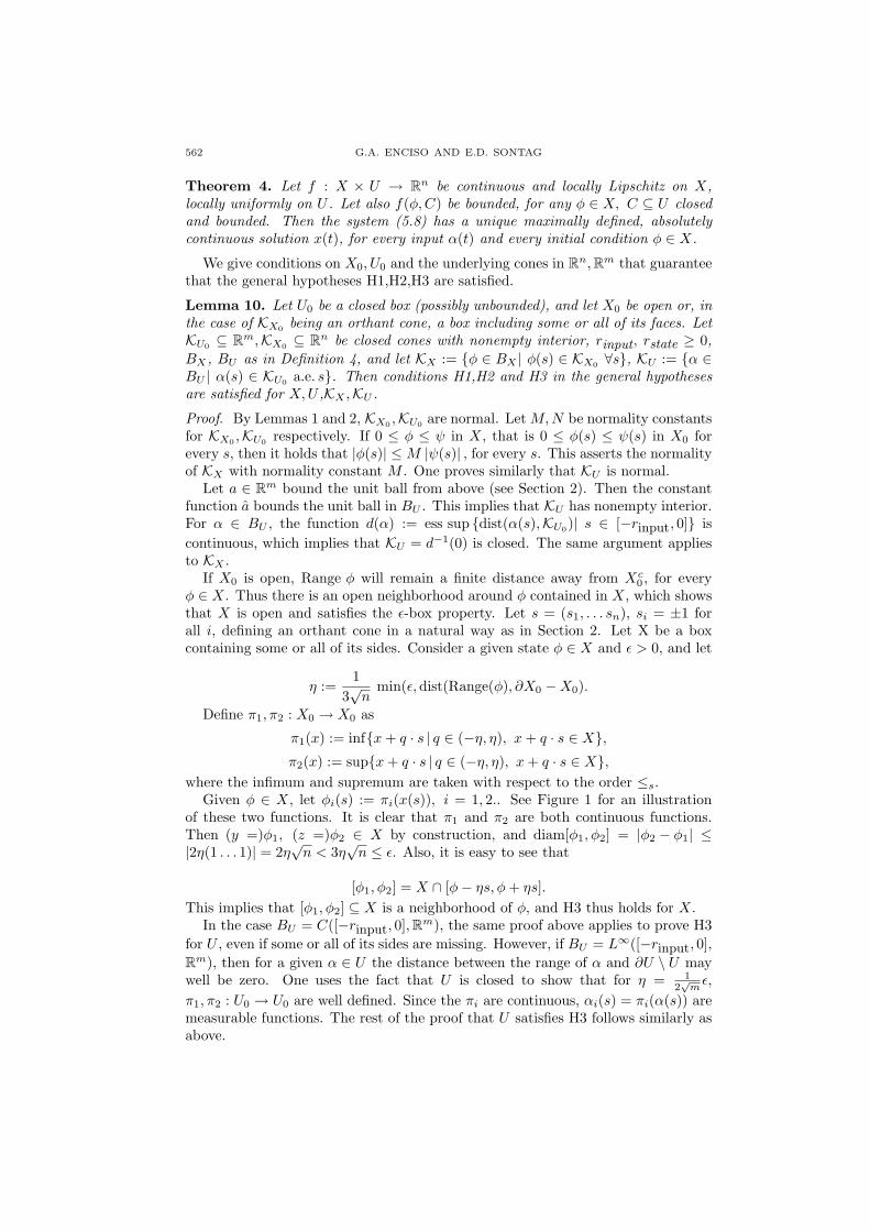
where the infimum and supremum are taken with respect to the order ≤s.Given φ ∈ X, let φi(s) := πi(x(s)), i = 1, 2.. See Figure 1 for an illustration

of these two functions. It is clear that π1 and π2 are both continuous functions.Then (y =)φ1, (z =)φ2 ∈ X by construction, and diam[φ1, φ2] = |φ2 − φ1| ≤|2η(1 . . . 1)| = 2η

√n < 3η

√n ≤ ε. Also, it is easy to see that

[φ1, φ2] = X ∩ [φ− ηs, φ + ηs].This implies that [φ1, φ2] ⊆ X is a neighborhood of φ, and H3 thus holds for X.

In the case BU = C([−rinput, 0],Rm), the same proof above applies to prove H3for U , even if some or all of its sides are missing. However, if BU = L∞([−rinput, 0],Rm), then for a given α ∈ U the distance between the range of α and ∂U \ U maywell be zero. One uses the fact that U is closed to show that for η = 1

2√

mε,

π1, π2 : U0 → U0 are well defined. Since the πi are continuous, αi(s) = πi(α(s)) aremeasurable functions. The rest of the proof that U satisfies H3 follows similarly asabove.


φ

φ1

φ2d3

d

Figure 1. Shown in the picture is the box X0 with one openand three closed faces, and φ1 ≤ φ ≤ φ2 in bold. Hered = dist(Range φ, ∂X − X0), and η = d/(3

√2). Note that

|φ(0)− φ1(0)| = |η(1, 1)| = d/3.

It will be proved that U satisfies H2. It is clear that U is closed and convex. Inthe case BU = C([−rinput, 0],Rm), and given a bounded set A ⊆ U , consider thebounded set A0 defined as the union of all the images of the functions in A. Use H2on A0 to find a, b ∈ U0 such that a ≤ A0 ≤ b. Then the constant functions a, b dothe same on the set A. In the case BU = L∞([−rinput, 0],Rm), the axiom of choiceallows to define A0, by picking a particular point-by-point defined function for eachu ∈ A. After possibly changing the values of each function at sets of measure zeroto ensure that A0 is bounded, the result follows as before. ¤

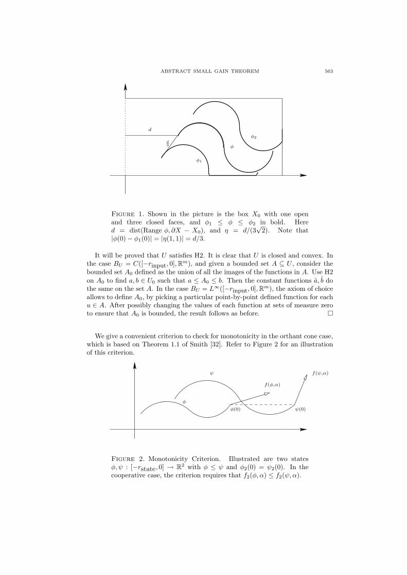
We give a convenient criterion to check for monotonicity in the orthant cone case,which is based on Theorem 1.1 of Smith [32]. Refer to Figure 2 for an illustrationof this criterion.

φ

ψ

φ(0) ψ(0)

f(φ,α)

f(ψ,α)

Figure 2. Monotonicity Criterion. Illustrated are two statesφ, ψ : [−rstate, 0] → R2 with φ ≤ ψ and φ2(0) = ψ2(0). In thecooperative case, the criterion requires that f2(φ, α) ≤ f2(ψ, α).


Proposition 1 (Monotonicity Criterion). Let (5.7) be a delay system, and let KX

be the orthant cone defined by the tuple s = (s1 . . . sn). Assume that i) α → f(φ, α)is an increasing function, for every φ ∈ X, and that ii) for every α ∈ U , φ ≤ ψ,and if φi(0) = ψi(0) for some i, it holds that sifi(φ, α) ≤ sifi(ψ, α). Then system(5.7) is monotone with respect to its underlying cones.

Proof. See the appendix for a sketch of the proof. ¤.

Suppose that the delay system (X, U, f) allows an I/S characteristic kX : U → X.Note that φ = Φ(t, kX(α), α) is constant over t, and thus that any solution of (5.7)with constant input α starting at kX(α) must satisfy xt = kX(α) for all t ≥ 0.This easily implies that kX(α) is a constant function, for every α. Hence, since kX

has a finite dimensional range, it is easy to verify when it is completely continuous,namely the image of every bounded set should be bounded. One can also think ofkX as having values in X0, and when evaluating un+1 = k(un) it is sufficient toconsider constant initial conditions.

In the applications of this paper the feedback function h : X → U will be definedas h(φ)(s) = h0(φ(s)), for some h0 : X0 → U0. In such case, it holds that u is itselfa constant vector. Also note that if z ∈ Rm is such that u ¿ k2(z) ¿ z, then theconstant function z has this property in U . Therefore one can apply Theorem 3 toprove stability in the context of delay systems.

To prove that Φ(t, φ, α) is a dynamical system, it is important to verify that thesemiflow condition is satisfied. To avoid confusion, this is best done for an abstractinput space U ; a short proof will be given in the appendix.Example. The following system corresponds to the cyclic gene model with repres-sion studied in [31]. Let y1 be a messenger RNA, which produces an enzyme y2,which produces another enzyme y3, and so on for p ≥ 2 steps. Let yp in turn inhibitthe production of y1, closing the cycle and inducing the repression. The system ismodeled as

y1 = F (Lpytp)− a1y1(t)

yi = Li−1yti−1 − aiyi(t), 2 ≤ i ≤ p,

(5.9)

where a1, . . . , ap > 0, F : [0,∞) → (0,∞) is a strictly decreasing continuous func-tion, and yt

i stands for the delay term yt used above, with superscripts to allowindexing. The delay is assumed to be r > 0 for all yi for simplicity. The operatorsLi are of the form

Liφ =∫ 0

−r

φ(s) dνi(s),

for positive Borel measures νi on [−r, 0], 0 < νi([−r, 0]) < ∞. Set X = C([−r, 0],(R+)p). Since F is decreasing, this system is not monotone. Nevertheless theinduced control system

y1 = F (Lpα(t))− a1y1(t)

yi = Li−1yti−1 − aiyi(t), 2 ≤ i ≤ p,

h(yt) = ytp = α(t),

(5.10)

will fit the setup of our results. Indeed, letting U = L∞([−r, 0],R+),4 the systemsatisfies the hypotheses of Theorem 4. It also fulfills the monotonicity criterion

4Here it is assumed that νi(E) = 0 whenever the Lebesgue measure of E ⊆ [−r, 0] is zero. Inthe case of point delays, one would set U = C([−r, 0],R+) as before.


using the cones KX = C([−r, 0], (R+)p), KU = L∞([−r, 0],R−) (note the negativesign). Lemma 10 is also satisfied, thus guaranteeing hypotheses H1-H3. Fixingα ∈ U , the control system can now be shown to converge towards the constantfunction (y1, . . . yp), where

y =(

F (Lpα)a1

, . . . ,F (Lpα)a1 · · · ap

).

To see this, note first that the convergence of y1 towards the constant functionF (Lpα)/a1 is elementary. The convergence of yt

2 towards (the constant function)F (Lpα)/(a1a2) is also evident, by considering the controlled linear system

y2 = β − a2y2(t),

where β(t) := L1yt1, and by noting that β(t) must converge. Inductively, the exis-

tence of the characteristic follows. Noting that kX sends bounded sets to boundedsets, it follows that H4 holds. The item 1 in the small gain condition holds clearly,since F is bounded (see next paragraph). To see that any solution y(t) of (5.9)is bounded, let z1(t) be a solution of z′ = F (0) − a1z, with initial conditionz1(0) = y1(0). Then y1(t) ≤ z1(t) for all t ≥ 0: to see this, note that the functionw(t) = z1(t) − y1(t) satisfies the equation w′(t) = F (0) − F (Lpα(t)) − a1w, whereF (0)− F (Lpα(t)) ≥ 0 and w(0) = 0. Now, since z1(t) is monotonic and convergestowards F (0)/a1, y1(t) is eventually bounded from above by F (0)/a1 + ε, for anyε > 0. In fact, F (0)/a1 is an upper hyperbound of y1(t) under the usual order. Theboundedness of y1(t) is used to carry out a very similar argument in order to showthat y2(t) is also eventually bounded, and the same holds for all other variables.This shows that all the solutions of the closed loop system are bounded.

By Theorem 2, system (5.9) is globally attractive whenever the discrete system

un+1 = k(un) =F (Lpun)

a1 · . . . · ap

is globally attractive. Note that even if u1 is a function, still u2, u3, . . . can beassumed to be constants, so that one can further reduce the system to be 1-dimensional. Whenever the hypotheses of Theorem 2 apply, the stability of thesystem is ensured by Theorem 3, the remainding hypotheses being trivially verified.The same procedure can be applied throughout to the coupled system of an oddnumber of repressions of the form (5.9), as done in Smith [31]. This is in accordwith the comments in p. 188 of that article:

The remarkable fact is that the dynamics of the two systems [discreteand continuous] appear to correspond both at the level of local stabilityanalysis and at the level of global dynamics. This is potentially a veryuseful fact, both for model construction and for analysis of particularmodels.

An example of a system (5) which is globally attractive is given by the functionF (x) := A/(K +x), for A, K > 0 arbitrary (the division by the constants a1 . . . ap ishere irrelevant). By Lemma 5, one only needs to show that the equation F (F (x)) =x has a unique solution. Such a solution would satisfy x = A/(K + F (x)), that is

A = Kx +Ax

K + x.


The right hand side is an increasing function that starts at the origin and growsto infinity; thus x is the unique intersection of this function with y = A, and thestatement follows.

6. A model of the lac operon. The following dynamical system was proposed byMahaffy and Savev [24] to describe the dynamics of lactose metabolism in E.Coli,which is orchestrated by the genes known as the lac operon. Some of the mainresults in [24] concern the global stability of the system; we will apply the smallgain theorem in its delay form to prove and extend these results.

The compounds involved in the system are the lac operon mRNA, the proteinsβ-galactoside permease, β-galactosidase (β-gal for short) and lactose, which aredenoted respectively by x1, x2, x3, x4. (Actually it is isolactose that regulates theoperon, but lactose and isolactose are considered identical in this model.) All sub-stances degrade at a fixed rate except for the lactose, which is actively digested bythe enzyme β-gal. The gene is activated whenever lactose is present in the system;more energetic sources of food, like glucose, are assumed not to be present. ThemRNA then induces the production of permease and β-gal, and the permease makesthe cell membrane more permeable to lactose, so that it can more efficiently enterthe cell. Mahaffy et al. assume that the production of mRNA has a natural satura-tion point, with Michaelis-Menten dynamics. This amounts to the presence of, say,a constant number of RNA polymerase molecules. After introducing an arbitrarydelay τ1 as a result of the transcription of x1, as well as a delay τ2 as a result of thetranslation of x2, x3, one can make a change of variables and arrive to the systemwith a single delay

x1(t) = g(x4(t− τ))− b1x1(t)

x2(t) = x1(t)− b2x2(t)

x3(t) = rx1(t)− b3x3(t)

x4(t) = Sx2(t)− x3(t)x4(t).

(6.11)

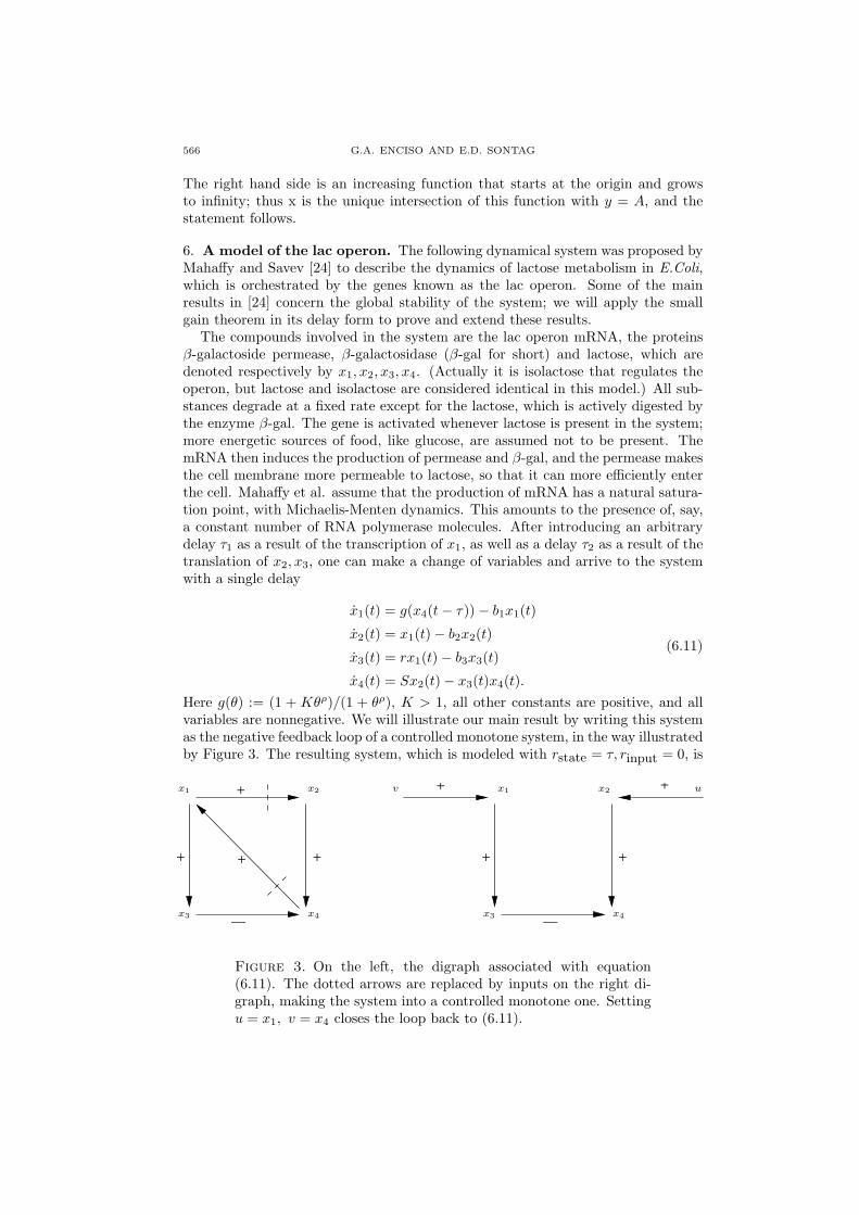
Here g(θ) := (1 + Kθρ)/(1 + θρ), K > 1, all other constants are positive, and allvariables are nonnegative. We will illustrate our main result by writing this systemas the negative feedback loop of a controlled monotone system, in the way illustratedby Figure 3. The resulting system, which is modeled with rstate = τ, rinput = 0, is

+

+

+

++

|

++

|

+x1 x2

x3 x4

x1 x2

x3 x4

v u

Figure 3. On the left, the digraph associated with equation(6.11). The dotted arrows are replaced by inputs on the right di-graph, making the system into a controlled monotone one. Settingu = x1, v = x4 closes the loop back to (6.11).


x1(t) = g(v(t))− b1x1(t)

x2(t) = u(t)− b2x2(t)

x3(t) = rx1(t)− b3x3(t)

x4(t) = Sx2(t)− x3(t)x4(t),

h(x(t)) = (x1(t), x4(t− τ)).

This model can be verified to be monotone with respect to the cones

KX = C([−rstate, 0],R+ × R− × R+ × R−), KU = R− × R+

using our monotonicity criterion. (In fact, monotonicity with respect to some or-thant cone is equivalent to the property that the associated digraph doesn’t haveany undirected closed loop with an odd number of ‘−’ signs.) See [2] for details,and Appendix I for a more systematic treatment in the finite dimensional case. Itis clear that the closed feedback loop of this system is (6.11).

It will be shown that this controlled system has a well defined characteristic, byappealing to Figure 3 and by noting that one can write the system as a cascade ofstable, one-dimensional systems. In fact, in the notation of (5.7), it holds in thisexample that f(xt, α) = f(x(t), α), and that the delay is only used for defining thefeedback function. If the delay in the state is ignored and the controlled system isviewed as a strictly finite dimensional system, it becomes obvious that a fixed control(u, v) will induce a globally asymptotically stable equilibrium, which is calculatedto be

x1 =g(v)b1

, x2 =u

b2, x3 =

r

b1b3g(v), x4 =

Sb1b3u

rb2g(v).After proving this, it is evident that the state kX(u, v) = (x1, x2, x3, x4) is a globallyasymptotically stable state. This proves the existence of the I/S characteristic. Thefeedback characteristic of the system is

k(u, v) =(

1b1

g(v),Sb1b3

rb2

u

g(v)

). (6.12)

To guarantee that this open loop system satisfies the hypotheses of the mainresult, let X0 = (R+)4, U0 = (R+)2, and note that Lemma 10 can be directly ap-plied to prove H1,H2,H3. The monotonicity and existence of the characteristic wasshown above, and since kX sends bounded sets to bounded sets (g(θ) is boundedfrom above by K and from below by 1), condition H4 also holds. Since the firstcomponent of k(u, v) is bounded from below and above by 1/b1 and K/b1 respec-tively, it is easy to see that the orbits of the discrete system (6.12) are uniformlybounded after two steps. Therefore item 1 in the small gain condition is satisfied. Tosee that a solution x(t) of system (6.11) is bounded, let z1(t), z2(t) be the solutionsof the systems z′ = 1 − b1z and z′ = K − b1z respectively, with initial conditionszi(0) = x1(0). It is easy to see that z1(t) ≤ x1(t) ≤ z2(t) for all t ≥ 0, see the previ-ous example. Since z1(t) (z2(t)) converges towards 1/b1 (K/b1), it holds that x1(t)is eventually bounded from below and above by fixed positive constants 1/b1 − εand K/b1 + ε respectively. In fact, 1/b1 (K/b1) is a lower (upper) hyperbound ofx1(t) in the usual order. Using this fact, the same procedure is used to show thatx2, x3 are bounded, and this in turn implies that x4 is also bounded (see also [24]).This shows that all the solutions of the closed loop system are bounded.

Note that k(u, v) has a unique fixed point u = 1b1

g(Sb3rb2

), v = Sb3rb2

. For any choiceof the parameters such that the discrete system (un+1, vn+1) = k(un, vn) is globally


attractive to this equilibrium, it follows from Theorem 2 that the original model(6.11) is globally attractive to its unique equilibrium. In those cases, the stability of(6.11) will be ensured by Theorem 3 and by the strict monotonicity of kX and h. Forthe remainder of this example, we will concentrate on finding sufficient conditionsfor the global attractivity of the discrete system.

In the global analysis of model (6.11), Mahaffy and Savev [24] restrict theirattention to the case ρ = 1, and they prove three results that provide sufficientconditions for global attractivity. We will come to the exact same conclusions, bywriting the system associated to (6.12) as a scalar discrete system of second order,and by appealing to the attractivity results known for such systems. For arbitraryρ we will also prove a new result, concerning global attractivity for any choice ofthe parameters b1, b2, b3, S and r, provided that an inequality holds for ρ,K. Letρ = 1, and consider the discrete system

(un+1, vn+1) = k(un, vn). (6.13)

It holds that un+1 = 1b1

g(vn), and

un+2 =1b1

g

(Sb1b3

rb2

un

g(vn)

)=

1b1

g

(Sb3

rb2

un

un+1

)=

βun+1 + γun

Bun+1 + Cun, (6.14)

where here ρ = 1 in g(θ), and β := 1b1

, γ := K Sb3rb1b2

, B := 1, C := Sb3rb2

. If theparameters of (6.14) are such that this discrete system has a globally attractiveequilibrium for all initial conditions u0, u1 > 0, then (6.13) has globally attractivesolutions for any initial condition u, v ≥ 0. (If u = 0 or v = 0, simply iterate (6.12)a few times and the states will become strictly positive.) The global attractivity of(6.13) clearly also implies that of (6.14).

The book by Kulenovic and Ladas [21] deals exclusively with rational discretesystems of second order. It follows from their treatment of equation (6.14) that forp := β/γ, q := B/C, and p < q, global attractivity holds (that is, with respect toarbitrary real initial conditions for which the iterations are well defined, including(u0, u1) ∈ (0,∞) × (0,∞)) if q < pq + 1 + 3p. Furthermore, instability occurs ifq > pq + 1 + 3p (see Theorem 6.9.1 in [21]).

In our case p = rb2KSb3

< rb2Sb3

= q, and attractivity holds if and only if

0 < q2 + 3q −Kq + K, q :=rb2

Sb3. (6.15)

For instance, if q < 1 then 0 < K−qK and thus (6.15) follows. This correspondsto Proposition 4.1 in [24]. Similarly, convergence follows whenever q > K, since then0 < q2−qK (Proposition 4.2 in [24]). Finally, for q > 1 equation (6.15) is equivalentto K < q(q + 3)/(q − 1), and the right hand side of this equation is bounded frombelow by 9. Thus for 1 ≤ K < 9 stability also follows. The remaining hypothesesin Theorem 4.3 of [24] can be shown to be equivalent to K < q(q + 3)/(q − 1) forq > 1. We summarize the three main global stability results of [24] in the followingstatement.

Theorem 5. For ρ = 1, the system (6.11) is globally attractive to a unique equi-librium, provided that 0 < q2 + 3q −Kq + K, q := rb2

Sb3. In particular, this holds if

q < 1, if q > K or if q > 1 and K < q(q + 3)/(q − 1). Whenever this condition issatisfied, system (6.11) is stable around this equilibrium.


The stability part of the above theorem is a direct consequence of Theorem 3,after noting that kX is ¿-increasing and h is ¿-decreasing, both of which arestraightforward to check.

Note that the delay τ was almost never used, and indeed can be arbitrarily largeor small. In fact, one can introduce different delays, large or small, in all of thefirst terms of the right hand sides of (6.11), and the results will apply with almostno variation. (If delays are introduced in the second terms, the systems will not bemonotone anymore.) If no delays are assumed, substantially stronger attractivityconditions hold; see [24].

Note that one can associate a second order, scalar discrete system to the originaltwo-dimensional system for any value of ρ, in the same way as above. One cor-respondence that can be easily verified by using equation (6.14) repeatedly is thefollowing: if u0 = u > 0 and u1 = v > 0, and if u0, u1 and (u, v) are taken as initialconditions of the systems (6.14) and (6.13) respectively, then u0, u1, u2, . . . generatesa two cycle in (6.14) if and only if (u, v) forms a two cycle in (6.13). Thus thereexist nontrivial two-cycles in (6.13) if and only if there exist nontrivial two cyclesin (6.14). For u = 0 or v = 0, similar comments apply as before. Recall that theexistence of nontrivial two-cycles in (6.13) is equivalent to the global attractivityof system (6.13), by Lemma 5 and the fact that this system is ≤-decreasing undersome orthant cone. By the above arguments, the same is true for system (6.14).Using the main result, the following proposition follows:

Proposition 2. The system (6.11) is globally attractive to its equilibrium wheneverthe only solution u > 0, v > 0 of the system of equations

u =βvρ + γuρ

Bvρ + Cuρ, v =

βuρ + γvρ

Buρ + Cvρ

is u = v = (β + γ)/(B + C), for β =1b1

, γ =K

b1

(Sb3

rb2

)ρ

, B = 1, C =(

Sb3

rb2

)ρ

.

This is a good point to comment on decomposing the same model as the nega-tive feedback loop of a monotone system in other ways – after all, one can see thatreplacing x3 by “u” in the fourth equation of (6.11), the resulting SISO system ismonotone as well. Indeed, in that way a characteristic k(u) can also be shown toexist, but it can be expressed only indirectly as the solution of a certain algebraicequation, since a directed loop remains in the digraph of the controlled system. Tocheck that there are no nontrivial two-cycles for the discrete system, it is necessaryto solve the system of equations u = k(v), v = k(u), which turns out to be equiv-alent and very similar to the system of equations in Proposition 2. Thus, there ismore than one way to decompose autonomous systems as closed loops of monotonecontrolled systems and use Theorem 2.

Next we provide sufficient conditions on K, ρ for system (6.11) to be globallyattractive, for any choice of the remaining parameters. We transform k(u, v) =(ζv, ξu/g(v)) into logarithmic coordinates. That is, consider

κ(σ, τ) := ln(k(eσ, eτ )).The initial condition (σ, τ) of the resulting discrete system is allowed to be an

arbitrary vector in R2. Then

κ(σ, τ) = (∆(τ), σ + c−∆(τ)), ∆(τ) := ln ζg(eτ ), c := ln ζξ.


Note that the iterations of this function converge globally to an equilibrium if andonly if those of k(u, v) do. To the former system one can associate the second ordersystem σn+2 = ∆(c + σn − σn+1) as was done in equation (6.14).

Lemma 11. Consider a discrete system σn+2 = ∆(c + σn − σn+1), where c isan arbitrary constant and ∆ is a bounded, non-decreasing, Lipschitz function withLipschitz constant α < 1/2. Then the system is globally attractive to its uniqueequilibrium σ = ∆(c).

Proof. It is clear that a constant sequence σ−1, σ0, σ1 . . . = σ is a solution ofthe discrete system if and only if σ = ∆(c), since σ0 = σ1 implies σ2 = ∆(c +σ0 − σ1) = ∆(c) and so on for all n ≥ 2 (the converse direction is evident). Leta0 := inf Range ∆, b0 := sup Range ∆. Then it holds that σn ∈ [a0, b0], n ≥ 1,for any initial conditions σ−1, σ0. Thus for all n ≥ 1,

σn − σn+1 + c ∈ [a0 − b0 + c, b0 − a0 + c],

and by calling a1 := ∆(a0 − b0 + c), b1 := ∆(b0 − a0 + c), it follows that σn ∈[a1, b1], n ≥ 3.

Define inductively ai+1 := ∆(ai − bi + c), bi+1 := ∆(bi − ai + c). Then for anyn ≥ 2i+1, σn ∈ [ai, bi], by induction on i as above. If one shows that |bi − ai| tendsto 0 as i increases, then the discrete system will be shown to be globally attractivetowards ∆(c), since ai ≤ ∆(c) ≤ bi for all i. Using the Lipschitz condition on ∆, itholds that

|bi−ai| = |∆(bi−1−ai−1+c)−∆(ai−1−bi−1+c)|≤ α |bi−1−ai−1+c−(ai−1−bi−1+c)|= 2α |bi−1 − ai−1| ≤ . . . ≤ (2α)i |b0 − a0| ,

and the conclusion follows. ¤In the particular case in question, it follows from the definitions of ∆(x) and g(θ)

that ∆(x) = ln ζ + ln(1 + keρx)− ln(1 + eρx). By derivating twice, it is shown that∆(x) has a unique inflexion point at x0 = − 1

2ρ ln K, and that

∆′(x0) =(K − 1)ρ

2(√

K + 1)<

12⇔ ρ <

√K + 1

K − 1,

and that ρ arbitrary if K = 1. The following corollary follows by the previouslemma and Theorem 2:

The following corollary follows by using the previous lemma and Theorem 2:

Corollary 3. The lac operon model (6.11) has a unique, globally attractive equi-librium for any choice of the positive parameters b1, b2, b3, r, S, provided that ρ <(√

K + 1)/(K − 1).

7. Appendix I: Decomposing Autonomous Systems into Negative Feed-back Loops of Monotone controlled Systems. It will be shown in this sectionthat, under rather general conditions, one can decompose an autonomous (not nec-essarily monotone) system into the negative feedback loop of a monotone controlledsystem. Sufficient conditions will also be found for the controlled system to havea well defined characteristic. This appendix is solely concerned with finite dimen-sional systems, where the ideas are most simply presented, but a generalization todelay systems is straightforward. Consider the controlled system

x = f(x, u), x ∈ X = (R+)n, u ∈ U = (R+)m, (7.16)


and fix a set S ⊆ 1, . . . n. Any vector (xi)i=1...n defines a vector xS = (xi)i∈S .Letting z stand for a fixed vector (zi)i∈SC , define the function fS(xS ; z, u) :=f(xS , z, u)S , where f(xS , z, u) is meant in the obvious sense. This vector fielddefines a controlled |S|-dimensional dynamical system

xS = fS(xS ; z, u) (7.17)

with n−|S|+m–dimensional control (z, u).Finally, denote by SC the complement 1,. . . , n - S of S. If π = S1, . . . SΛ is

a partition of 1 . . . n, then the coupled system

xSλ = fSλ(xSλ ;xSCλ , u), λ = 1 . . . Λ (7.18)

is equivalent to (7.16).Sign Definite Systems. Many dynamical systems arising from gene and proteinmodels can be associated with a signed digraph. Given an autonomous system

x = g(x), x ∈ X = (R+)n, (7.19)

let the variables x1 . . . xn be vertices, and write a positive arc from xi to xj , i 6= j,if ∂

∂xigj(x) ≥ 0 for all x ∈ X and the strict inequality holds at least at some state.

Similarly, write a negative arc from xi to xj if ∂∂xi

gj(x) ≤ 0 (with strict inequalityat some state), and no arc if ∂

∂xigj(x) ≡ 0. Note that not every system satisfies this

trichotomy for all its variables. The attention will be restricted in this appendix tosuch systems, which will be denoted as sign definite.

If the system (7.19) is sign definite with associated digraph G, then one can findan n-dimensional controlled system

x = f(x, u), x ∈ X = (R+)n, u ∈ U = (R+)m, h : X → U, (7.20)

which is i) monotone with respect to some orthant cones in the inputs and thestates; ii) such that the function h is ≤-decreasing; and iii) such that its closed loopsystem is well defined and is (7.19). This will be done as follows, trying to minimizethe number of inputs and outputs involved so as to make the reduced model inTheorem 2 as simple as possible.

Let A ⊆ x1, . . . xn be an arbitrary set of variables, called agonists. These vari-ables may be unrelated to each other, but it is best (and most meaningful) to choosethem so that their dynamics are positively correlated, i.e. most arrows connectingtwo nodes from A are positive. The remaining variables will be referred to as an-tagonists, and they will also be thought of as being mostly positively correlated toeach other.

An arc in G will be called discordant if it is positive and joins an agonist withan antagonist, or if it is negative and joins two agonists or two antagonists. LetDj := xi| there is a discordant arc from xi to xj, and let D :=

⋃j Dj , m := |D|

and U := (R+)m. Now enumerate the elements of D as xl1 , . . . , xlm . Define fj(x, u)as the result of replacing in gj(x) all appearances of xli by ui, for each xli ∈ Dj . Thecontrolled system (7.20) thus defined has a state digraph G′ that can be describedas the result of removing all discordant arcs from G.

Now define the output function h : X → U as hk(x) := xlk , k = 1 . . . p, and closethe loop by letting u(t) = h(x(t)). Let

s(i) :=

1 if xi ∈ A−1 if xi 6∈ A


and let KX be the orthant cone induced by s. Let pk := −slk , k = 1 . . .m, and letKU be the orthant cone defined by p.Example. Equation (6.11) and Figure 3 form a good example of these definitions.In this model, one can consider as agonists the variables x1, x3 and as antagonistsx2, x4. There are only two discordant arcs and it holds that D1 = x4, D2 =x1, D3 = D4 = ∅; thus D = x1, x4. The variables x1 and x4 are replaced by uand v in the functions g2, g1 to form the functions f2(x, u), f1(x, v), respectively.

An important consideration in making the choice of the agonist set is to minimizethe number of inputs. See Figure 4 for an example of a system in which the agonistset is chosen in two different ways.

+ |

|

| +

|

++

+

| +

b

a

a

a a

b

|

|

| +

|

+

+

| +

a

aa

b

bb

b +b

+

Figure 4. Network Splitting. The nodes in the digraphs abovehave been labelled “a” for agonist and “b” for antagonist in twodifferent ways, and the discordant arrows have been circled in eachcase. The nodes at the base of these arrows will form the set Dof inputs of the controlled system (four inputs in the first digraph,and two in the second). Note that by choosing the agonists andantagonists in an educated way one can substantially reduce thenumber of inputs.

Before providing our construction leading to i),ii),iii), the following simple resultis stated and proved for convenience. Given a digraph H, we denote by V (H) theset of vertices of H, and by A(H) the set of arcs of H.

Lemma 12. Let H be an acyclic digraph. Then there exists a bijection b : V (H) →1, . . . |V (H)| such that (v1, v2) ∈ A(H) implies b(v1) < b(v2).

Proof. The proof proceeds by induction on the number of vertices. If there is onlyone vertex, the bijection is trivial. Assuming the statement true for graphs of atmost n vertices, let H have n + 1 vertices. There exists at least one vertex v withno incoming arcs. Remove it and apply the statement on the remaining digraph H ′

to form a bijection b : V (H ′) → 2, . . . n + 1. Finally, define b(v) := 1. The resultfollows. ¤

Theorem 6. The controlled system (7.20) described above is monotone, and h isa ≤-decreasing function. The closed loop system of (7.20) is well defined and equalto system (7.19). Furthermore, if for each strongly connected component of G′ with


vertices S ⊆ 1 . . . n the system (7.17) has a well defined I/S characteristic, then(7.20) allows an I/S characteristic.

Proof. The Kamke monotonicity criterion for controlled systems will be used:given orthant cones KX and KU generated by the tuples (s1, . . . sn) and (p1, . . . pm)respectively, a system (7.20) is monotone with respect to these cones if and only if

sjsi∂fj

∂xi≥ 0, ∀i 6= j and sjpk

∂fj

∂uk≥ 0, ∀i, k, (7.21)

where i, j = 1 . . . n and k = 1 . . .m; see [32, 2]. To prove the first assertion in7.21, let i 6= j be such that there is an arc from xi to xj in G′ (otherwise there isnothing to prove). Then either both variables are agonists and the arc is positive,or both are antagonists and the arc is also positive, or else one is agonist, one isantagonist and the arc is negative. In all these cases, the first statement in (7.21)is satisfied. As to the second statement, if k, j are such that ∂fj/∂uk 6≡ 0, then byconstruction the arc from xlk to xj in G is discordant, so that slksj∂gj/∂xlk ≤ 0.Also by construction, sign ∂gj/∂xi = sign ∂fj/∂uk. Therefore sjpk∂fj/∂uk ≥ 0 asexpected.

Recall that pk = −slk , hk(x) = xlk to see that h is ≤-decreasing. Replacing eachuk in fj(x, u) back with hk(x) = xlk will form back gj(x). This proves that theclosed loop system is the same as (7.19).

For the last assertion write (7.20) as a cascade of controlled monotone systemson the state spaces Xλ := (R+)|Sλ|, λ = 1 . . . Λ, where S1, . . . , SΛ are the stronglyconnected components (s.c.c.) of G′. Let H be the acyclic digraph with verticesS1 . . . DΛ which is naturally induced by the digraph G′, i.e. (Sλ, Sµ) ∈ A(H) if andonly if (x, y) ∈ A(G′) for some x ∈ Sλ, y ∈ Sµ. Now use Lemma 12 to relabel thes.c.c’s in such a way that if xi ∈ Sλ1 , xj ∈ Sλ2 , and there is an arc from xi to xj ,then λ1 ≤ λ2.

Consider the function fS1(xS1 ; z, u), where z = (zi)i∈SC1

is given. By the choiceof S1, it holds that fS1 doesn’t actually depend on z, and it can be written asfS1(xS1 , u). Similarly one can write fSλ(xSλ ; xSC

λ , u) in (7.18) as

fSλ(xSλ ; xS1 , . . . xSλ−1 , u),

and thus system (7.20) is written as a cascade as desired, using equation (7.18).Given a fixed input u ∈ U , the system xS1 = fS1(xS1 ;u) converges globally

towards a vector (xi)i∈S1 , by hypothesis. Using u1, . . . um and the variables in S1

as inputs, the system

xS2 = fS2(xS2 ;xS1 , u)

can be seen to satisfy (7.21), since some of the variables have now been simply rela-belled as inputs. Also, this system has a well-defined characteristic by hypothesis.Thus the property CICS holds, and since (xS1 , u) converges to (xS1 , u), then xS2

converges to xS2 . The same argument holds to show that all the cascade converges,thus proving that system (7.20) has an I/S characteristic. ¤

Corollary 4. If the digraph G′ associated to system (7.20) is acyclic, and for everyi = 1 . . . n the 1-dimensional system

xi = gi(x1, . . . , xi−1, xi, xi+1, . . . , xn)


with controls xj , j 6= i, has a well defined I/S characteristic, then (7.20) allows anI/S characteristic.

Proof. The graph G′ is acyclic, therefore its strongly connected components areexactly the singletons 1, . . . , n. By the previous theorem, the result follows. ¤

Discussion. The reader will notice a tradeoff in the number of variables chosento form the input: the more variables are included in D, the more complex is theresulting discrete system in SGT, but the less connected is G′ and the easier to showthe existence of a characteristic. Note that D is completely determined by the set Aof agonists, which is arbitrary and allows for some choice. The results in this sectionmake SGT robust to possible changes in the model. If a new participating gene isdiscovered as part of a gene network, one can simply keep the previous agonists,introduce the new gene either as agonist or antagonist, and obtain a monotonesystem (7.20) that has a similar topology as the previous one. The second conditionin Theorem 6, regarding the existence of the characteristic, also needs to be checkedonly locally if a new node or a new arrow is introduced.

8. Appendix II.

8.1. Existence and Uniqueness.

Theorem 7. Let X0 ⊆ Rn be an open set, or in the orthant cone case, a box (notnecessarily bounded) containing some or all of its sides. Let BU be a Banach space,and let U ⊆ BU be an arbitrary Borel measurable set. Let X = C([−r, 0], X0), andlet f : X × U → Rn be a continuous function. Assume that

i): f is locally Lipschitz on X, locally uniformly on U : for any C ⊆ U andD ⊆ X closed and bounded, there exists M > 0 such that

|f(φ, α)− f(ψ, α)| ≤ M |φ− ψ| , ∀φ, ψ ∈ D,∀α ∈ C.

ii): There exists φ0 ∈ X such that for all C ⊆ U closed and bounded, the setf(φ,C) is bounded.

Then the system (5.8) has a unique maximally defined, absolutely continuous solu-tion x(t) for every input β ∈ U∞ and every initial condition φ ∈ X.

Proof. It will be shown that all hypotheses are met so as to apply Theorem 4.3.1,p. 207 of Bensoussan et al. [4]. Let Ω0 ⊆ X0 be a given compact set, and letΩ = C([−r, 0],Ω0). Let Ci := B(0, i) ∩ U , where i = 1, 2, 3 . . . and B(0, i) isthe open ball in BU with radius i. For every Ci, there is a constant Mi suchthat f(·, α) is Mi-Lipschitz on Ω, for all α ∈ Ci. For any α ∈ U , let m(α) :=infMi | i such that α ∈ Ci. Note that f(·, α) is m(α)-Lipschitz on Ω for each αand that m is measurable. Indeed, each Mi can be chosen to be as small as possible,and then m becomes a step function on each Ci.

Now for every fixed α ∈ U , extend the function φ 7→ f(φ, α) from Ω to all of BX ,in such a way that the extension is also m(α)-Lipschitz. For this, let

Fi(φ, α) := infψ∈Ω0

fi(ψ, α) + m(α) |φ− ψ| ,for each i, and let F = (F1, . . . , Fn). It is a simple exercise in analysis to verifythat for a fixed α, F (·, α) is well defined, coincides with f(·, α) on Ω, and is itself√

nm(α)-Lipschitz.Fix now β ∈ U∞, and define g(t, φ) := F (φ, β(t)). It is to this function that

Theorem 4.3.1 of [4] is applied. A few conditions need to be verified: F is continuous


on each set X × (Ci − Ci−1)) and therefore measurable, which implies that g(t, φ)is also measurable. By setting n(t) = m(β(t)), it follows that n(t) is measurableand locally bounded (since each β|[0,T ] is contained in some Ci), and thus locallyintegrable. Finally, note that F (φ0, Ci) is bounded in Rn for every i, and thattherefore t → g(t, φ0) is locally integrable.

By Theorem 4.3.1 in [4], the system x = g(t, xt) = F (xt, β(t)) has a uniquemaximally defined, absolutely continuous solution defined for every initial conditionφ ∈ BX .

Next define for a fixed initial condition φ ∈ X, and j = 1, 2, 3, . . .:

Ωj := Range(φ) ∪ x ∈ X0 |dist(x, Range(φ)) ≤ j and dist(x, ∂X \X) ≥ 1/j.Extend f from Ωj to all Rn to form Fj , applying the main step above. The solutionsof the systems x = Fj(xt, β(t)), j = k, k + 1, . . ., using the same initial conditionφ, must agree with each other by uniqueness. If x1(t), x2(t) are both solutions of(5.8) with initial condition φ and are defined on [0, T ], let j be such that x1|[−r,T ] ∪x2|[−r,T ] ⊆ Ωj . Then x1 = x2 on [−r, T ] by the argument above. This shows thatx(t) is unique. The fact that it is maximally defined follows similarly. ¤

8.2. Proof of Lemmas 1 and 2.Proof of Lemma 1: Let K have nonempty interior, that is 0 ≤ Bε(x0) for somex0 > 0 and some real ε > 0. Then 0 ≤ B1(ε−1x0), which is equivalent by definitionto B1(0) ≤ ε−1x0. The converse result follows by the same argument. ¤Proof of Lemma 2: Let C1 := x ∈ K| |x| = 1. Let f : C1×C1 → R, f(x, y) :=x · y. C1 is compact, therefore f must have a minimum at some (x0, y0). Butf(x0, y0) > −1, since otherwise x0 = −y0 and a contradiction would follow fromK ∩ (−K) = 0. If follows that there is θ < 1 such that x · y ≥ −θ |x| |y|, for everyx, y ≥ 0.

Now let 0 ≤ x ≤ y. Then (y − x) · x ≥ −θ |x| |y − x|, so

|x|2 ≤ θ |x| |y − x|+ x · y ≤ |x| (θ |x|+ θ |y|+ |y|),and after cancelling |x| on both sides (if x = 0 there is nothing to prove) and solvingfor |x|, one has

|x| ≤ θ + 1θ − 1

|y| .¤

8.3. Monotonicity Criterion and Semiflow Property.Sketch of Proof for Proposition 1. Let α, β be two inputs, and assume α(t) ≤β(t) for every t (if this only holds a.e. t, one can change the value of these func-tions at a set of measure zero). Let h1(t, φ) := f(φ, α(t)), h2(t, φ) := f(φ, β(t)).Theorem 1.1 of Smith [32] cannot be applied directly, even in the cooperative case,since the functions hi are not necessarily continuous on t. Nevertheless by writingthe absolutely continuous solution x(t, φ;hi) of x = hi(t, xt) as an integral (seeBensoussan et al. [4]) one shows that, for e À 0 in X and hε

i(φ, t) := εe + hi(φ, t),x(t0, φ; hε

i) converges towards x(t0, φ; hi) as ε → 0 for each t0. The rest of the ar-gument is as in [32]: define e := (s1, s2, . . . sn) À 0. Show by contradiction thatx(t, φ; h1) ¿ x(t, φ; hε

2) for all t and small ε, and let ε tend to zero. ¤The following two lemmas give a proof that the function Φ(t, φ, α) = xt satisfies

the semiflow property. The proof is straightforward, but it is included because theresult might seem counterintuitive for delay systems. Let BU be an abstract Banach


space here, and U ⊆ BU . Consider X0 ⊆ Rn, X = C([−r, 0],Rn) as before, andf : X × U → Rn such that the triple (X,U,f) forms a well defined delay dynamicalsystem as in Definition 4.

Lemma 13. Let u, v be inputs in U such that u(t) = v(t), 0 ≤ t ≤ t0. Then thesolutions x(t), y(t) of the system (5.7), with initial condition φ0 and inputs u andv respectively, satisfy x(t) = y(t),−r ≤ t ≤ t0.

Proof: Let γ(t) := v(t + t0), and let z(t) be the solution of (5.7) with input γ andstarting condition φ1 = xt0 . Let w(t) := x(t) for −r ≤ t ≤ t0, w(t) := z(t − t0)for t > t0. It is easy to see that w(t) is absolutely continuous, as it is built fromabsolutely continuous parts. Further,

w′(t + t0) = z′(t) = f(γ(t), zt) = f(v(t + t0), w(t + t0)), a.e. t ≥ 0.

Thus w(t) is a solution of (5.7) with input v(t) (recall u(t) = v(t),−r ≤ t ≤ t0), andinitial condition φ0. By uniqueness, it must hold that w = y, and the conclusionfollows.

Lemma 14 (Semiflow Property). Given s, t ≥ 0, and inputs u(τ), v(τ), let x(τ), y(τ)be the solutions of (5.7) with inputs u1(τ), u2(τ) respectively, and initial conditionsφ and xs respectively. Let z(τ) be the solution of (5.7) with initial condition φ andinput v(τ) := u1(τ), 0 ≤ τ ≤ s, v(τ) := u2(τ − s), τ > s. Then zs+t = yt.

Proof. By the previous Lemma, zs = xs. Note that w(t) := z(s + t) is a solutionof (5.7) with input u and initial condition xs:

w′(τ) = z′(s + τ) = f(v(s + τ), z(s + τ) = f(u2(τ), w(τ)), ∀τ ≥ 0.

Thus w = y by uniqueness. In particular, yt = wt = zs+t. ¤

Acknowledgements. We wish to acknowledge David Angeli for his many sugges-tions on how to work out the stability of discrete systems, Patrick de Leenheer formany discussions, and especially Hal Smith for very useful discussions and sugges-tions. We also want to acknowledge the multiple comments and suggestions of thereviewers, who helped to substantially improve the quality of the text.

REFERENCES

[1] D. Aeyels and P. De Leenheer, Stability for homogeneous cooperative systems, Proc. IEEEConf. Decision and Control, Phoenix, pp. 5241-5242, 1999.

[2] D. Angeli, E.D. Sontag, Monotone control systems, IEEE Trans. Autom. Control, 48: 1684-1698, 2003.

[3] D. Angeli, E.D. Sontag, Multistability in monotone input/output systems, Systems and Con-trol Letters 51:185–202, 2004.

[4] A. Bensoussan, G. Prato, M.C. Delfour, and S.K Mitter, “Representation and Control ofInfinite Dimensional Systems”, Birkhauser, Boston, 1992.

[5] Y. Chitour, F. Grognard, G. Bastin, Stability Analysis of a Metabolic Model with SequentialFeedback Inhibition, in “First Multidisciplinary International Symposium on Positive Systems:Theory And Applications” (Posta 2003), Rome, August 2003 (L. Benvenuti, A. De Santis,and L. Farina, eds.), Springer-Verlag, Heidelberg, pp. 143-150, 2003.

[6] S.N. Chow, J. Mallet-Paret, Singularly perturbed differential equations. In: J. Chandra, A.C.Scott (eds), ”Coupled Nonlinear Oscillators”, North-Holland, Amsterdam, 1983.

[7] E.N. Dancer, Some remarks on a boundedness assumption for monotone dynamical systems,Proc. of the AMS 126:801-807, 1998.

[8] C.A. Desoer, M. Vidyasagar, “Feedback Synthesis: Input-Output Properties”, AcademicPress, New York, 1975.


[9] G.A. Enciso, E.D. Sontag, Monotone systems under positive feedback: multistability and areduction theorem, Systems and Control Letters 51(2):185-202,2005.

[10] G.A. Enciso, E.D. Sontag, On the stability of a model of testosterone dynamics, Journal ofMathematical Biology 49:627-634,2004.

[11] L. Farina and S. Rinaldi, “Positive Linear Systems: Theory and Applications”, John Wiley& Sons, New York, 2000.

[12] J.-L. Gouze, Differential Systems with Positive Variables, in “First Multidisciplinary Inter-national Symposium on Positive Systems: Theory And Applications” (Posta 2003), Rome,August 2003 (L. Benvenuti, A. De Santis, and L. Farina, eds.), Springer-Verlag, Heidelberg,pp. 151-158, 2003.

[13] J.K. Hale, “Introduction to Functional Differential Equations”, Springer, New York, 1993.[14] M.W. Hirsch, Stability and convergence in strongly monotone dynamical systems, Reine und

Angew. Math. 383:1-53, 1988.[15] B. Ingalls and E.D. Sontag, A small-gain theorem with applications to input/output systems,

incremental stability, detectability, and interconnections, J. Franklin Institute 339:211-229,2002.

[16] J. Ji-Fa, On the global stability of cooperative systems, Bull. London Math. Soc. 26:455-458,1994.

[17] Z.P. Jiang, A. Teel, L. Praly, Small-gain theorem for ISS systems and applications, Mathe-matics of Control, Signals, and Systems 7:95-120, 1994.

[18] J. Keener, J. Sneyd, “Mathematical Physiology”, Springer, New York, 1998.[19] T. Kobayashi, L. Chen, K. Aihara, Modeling genetic switches with positive feedback loops,

J.Theor.Biol. 221:379-399, 2003.[20] V.L. Kocic, G. Ladas, “Global Behavior of Nonlinear Difference Equations of Higher Order

with Applications”, Kluwer Academic, Boston, 1993.[21] M.R.S. Kulenovic, G. Ladas, “Dynamics of Second Order Rational Difference Equations”,

Chapman & Hall/CRC, New York, 2002.[22] P. de Leenheer, D. Angeli, E.D. Sontag, A tutorial on monotone systems with an application

to chemical reaction networks, Proc. 16th Int. Symp. Mathematical Theory of Networks andSystems (MTNS), 2004.

[23] J. Mallet-Paret, R.D. Nussbaum, Global continuation and asymptotic behavior for periodicsolutions of a differential-delay equation. Ann. Mat. Pura. App. (IV) CXLV:33-128, 1986.

[24] J.M. Mahaffy, E.S. Savev, Stability analysis for a mathematical model of the lac operon,Quarterly of Appl. Math, LVII,1:37-53, 1999.

[25] I.M.Y. Mareels, D.J. Hill, Monotone stability of nonlinear feedback systems, J. Math. Systems,Estimation and Control 2:275-291, 1992.

[26] J.D. Murray, “Mathematical Biology, I: An introduction”, Springer, New York, 2002.[27] C. Piccardi and S. Rinaldi, Remarks on excitability, stability, and sign of equilibria in coop-

erative systems, Systems and Control Letters 46:153-163, 2002.[28] E.P. Ryan, E. Sontag, “A counterexample on steady state responses and the converging-input

converging-state property,” in preparation.[29] M. Safonov, “Stability and Robustness of Multivariable Feedback Systems”, The MIT Press,

Cambridge, Massachusetts, 1980.[30] I.W. Sandberg, On the L2-boundedness of solutions of nonlinear functional equations, Bell

System Technical Journal 43:1581-1599, 1964.[31] H.L. Smith, Oscillations and multiple steady states in a cyclic gene model with repression, J.

Math. Biol. 25:169-190, 1987.[32] H.L. Smith, “Monotone Dynamical Systems”, AMS, Providence RI, 1995.[33] E.D. Sontag, “Mathematical Control Theory”, Springer, New York, 1998.[34] E.D. Sontag, Smooth stabilization implies coprime factorization, IEEE Trans. Automatic

Control 34:435-443, 1989.[35] G. Stepan, “Retarded Dynamical Systems: Stability and Characteristic Functions”, Wiley,

New York, 1989.[36] E.D. Sontag, Asymptotic amplitudes and Cauchy gains: A small-gain principle and an ap-

plication to inhibitory biological feedback, Systems and Control Letters 47:167-179, 2002.[37] J.J. Tyson, H.G. Othmer, The dynamics of feedback control circuits in biochemical pathways.

In: R. Rosen, F.M. Snell (eds), ”Progress in Theoretical Biology”, Academic Press, New York,1978.


[38] G. Zames, On the input-output stability of time-varying nonlinear feedback systems. Part I:Conditions using concepts of loop gain, conicity, and positivity, IEEE Trans. Autom. Control11:228-238, 1966.

Received October, 2004; 1st revision December 2004; 2nd revision March 2005.E-mail address: [email protected]

E-mail address: [email protected]

global attractivity, i/o monotone small-gain...

Documents