JHEP08(2014)146

Published for SISSA by Springer

Received: May 13, 2014

Accepted: July 27, 2014

Published: August 26, 2014

Global aspects of abelian duality in dimension three

Chris Beasley

Department of Mathematics, Northeastern University,

360 Huntington Ave, Boston, MA 02115, U.S.A.

E-mail: C.Beasley@neu.edu

Abstract: In three dimensions, an abelian gauge field is related by duality to a free,

periodic scalar field. Though usually considered on R3, this duality can be extended to

a general three-manifold M , in which case topological features of M become important.

Here I comment upon several of these features as related to the partition function on M .

In a companion article, I discuss similarly the algebra of operators on a surface of genus g.

Keywords: Field Theories in Lower Dimensions, Wilson, ’t Hooft and Polyakov loops,

Duality in Gauge Field Theories, Differential and Algebraic Geometry

ArXiv ePrint: 1405.2123

Open Access, c© The Authors.

Article funded by SCOAP3.doi:10.1007/JHEP08(2014)146

JHEP08(2014)146

Contents

1 Introduction 1

2 Analysis of the abelian sigma model 5

2.1 The classical sigma model 6

2.2 Computing the partition function 9

3 Analysis of the abelian gauge theory 15

3.1 The classical Maxwell theory 15

3.2 Computing the partition function 19

4 Modularity, duality, and all that 27

4.1 A theta-function for three-manifolds 27

4.2 The role of torsion 30

5 Path integral explanation 36

5.1 Duality for the partition function 36

5.2 Duality for operators 39

1 Introduction

In classical field theory, abelian duality amounts to a simple relation between the solutions

of certain linear partial differential equations on Rn for n ≥ 2. The most elementary ex-

ample occurs in dimension two, for which one considers a harmonic function φ ∈ C∞(R2)

satisfying the Laplace equation

φ = d†dφ = 0 , d† = − ⋆ d ⋆ . (1.1)

Here ⋆ is the Hodge star operator determined by the Euclidean metric on R2.

According to (1.1), the one-form ⋆dφ is closed. Since R2 has trivial cohomology in

degree one, ⋆dφ is also exact. Hence one can associate to φ another function ψ ∈ C∞(R2)

via the duality relation

⋆ dφ = dψ . (1.2)

The relation in (1.2) determines the function ψ up to the addition of a constant, and ψ is

automatically harmonic by virtue of the identity

ψ = d†dψ = ⋆d2φ = 0 . (1.3)

The classical duality in (1.2) thus relates one solution of the Laplace equation on R2 to

another, distinct solution. As well-known, the dual harmonic functions φ and ψ can be

combined as the real and imaginary parts of a single holomorphic function on R2 ≃ C.

– 1 –

JHEP08(2014)146

Similarly in dimension four, if A is a U(1)-connection on R4 which solves the source-free

Maxwell equation

d ⋆ FA = 0 , FA = dA , (1.4)

then A determines another U(1)-connection B up to gauge equivalence via

⋆ FA = FB . (1.5)

By virtue of the Bianchi identity dFA = 0, the curvature of the connection B also satisfies

d ⋆ FB = 0, so the classical electric-magnetic duality in (1.5) relates distinct solutions of

the source-free Maxwell equation on R4.

In this paper we are concerned with abelian duality in dimension three. In that case,

classical abelian duality relates a U(1)-connection A which solves the Maxwell equation on

R3 to a harmonic function φ on R

3. By analogy to dimensions two and four, the classical

duality relation in dimension three is

⋆ FA = e2 dφ . (1.6)

Unlike the preceding duality relations, the classical duality relation on R3 involves the

electric coupling e2, which appears in the Maxwell action

I(A) =1

4πe2

∫

R3

FA ∧ ⋆FA ,

=1

8πe2

∫

R3

d3x√g FA,mn F

mnA , m, n = 1, 2, 3 . (1.7)

The factor of 1/4π in the first line of (1.7) is simply a notational convenience, which will

eliminate other factors later. In the second line of (1.7), we rewrite the Maxwell action

in components with respect to an arbitrary Riemannian metric g on R3, and we follow

the standard Einstein convention in summing over the repeated indices m and n on the

curvature FA of the gauge field.

The appearance of the Maxwell coupling e2 in the duality relation (1.6) is the first of

several peculiarities specific to dimension three. Most famously, the duality relations in two

and four dimensions are invariant under conformal transformations, which preserve both

the one-form ⋆dφ on R2 in (1.2) and the two-form ⋆FA on R

4 in (1.5). But in dimension

three, if the metric g is scaled by a constant factor

g 7−→ Λ2 g , Λ ∈ R+ , (1.8)

the dual one-form ⋆FA in (1.6) scales non-trivially as well,

⋆ FA 7−→ Λ−1 ⋆ FA . (1.9)

In components, ⋆FA is given by√g ǫmnp F

mn dxp, where ǫmnp is the anti-symmetric tensor

on three indices, with fixed normalization ǫ123 = +1. The scaling for ⋆FA in (1.9) follows

from the combined scalings of√g with weight Λ3 and Fmn with weight Λ−4. As a result,

neither the duality relation in (1.6) nor the classical Maxwell action in (1.7) is invariant

under scale, much less conformal, transformations of the metric on R3.

– 2 –

JHEP08(2014)146

On the other hand, if the transformation of the metric in (1.8) is supplemented by a

non-trivial scaling for the electric coupling e2 itself,

e2 7−→ Λ−1 e2, (1.10)

then the Maxwell action on R3 is invariant. Because ⋆FA and e2 transform with identical

weights, the abelian duality relation in (1.6) is also preserved under scaling. Conversely, the

appearance of e2 in the duality relation is dictated by invariance under the transformations

in (1.8) and (1.10).

Each of the classical duality relations in (1.2), (1.5), and (1.6) extends to an equivalence

of free quantum field theories defined on an arbitrary Riemannian manifold Σ, X, or M of

corresponding dimension two, four, or three. Though the relevant pairs of quantum field

theories are themselves trivial, the equivalence between them is generally non-trivial and

may depend in interesting ways on the topology of the underlying manifold.

These topological issues are particularly sharp when M is a closed three-manifold.

In that case, the global analysis of the classical Laplace equation on M is very different

from the global analysis of the classical Maxwell equation on M . Solutions to the Laplace

equation will be unique up to scale, but solutions to the Maxwell equation generically

fall into continuous families, parametrized by the holonomies of the gauge field. So on a

general three-manifold, there is no hope to interpret abelian duality classically, as a one-to-

one correspondence (1.6) between solutions of the Laplace and Maxwell equations on M .

Instead, abelian duality on M must be interpreted as an inherently quantum phenomenon.

A basic observable in any quantum field theory is the partition function, and as an

initial question, one can ask how the partition function transforms under duality. Naively,

one might expect the partition function to be invariant under duality, but famously in

dimensions two and four, this is not so.

The most elegant statement [35] occurs for electric-magnetic duality of Maxwell theory

on a four-manifoldX. (See also [33] for related observations.) In this case, the Maxwell par-

tition function ZX depends upon both the Maxwell coupling e2 and an angular parameter

θ which enters the classical Lagrangian through the topological pairing

Iθ(A) =i θ

8π2

∫

XFA ∧ FA ,

=i θ

32π2

∫

Xd4x

√g ǫmnpq F

mnA F pq

A .

(1.11)

When X is a spin-manifold, the normalization in (1.11) ensures that θ has period 2π.

Otherwise, θ has period 4π.

The angular parameter θ naturally complexifies the electric coupling e2 via

τ =θ

2π+

4πi

e2, (1.12)

and electric-magnetic duality acts upon τ as a modular transformation τ 7→ −1/τ . More-

over, as shown by direct computation in [35], the Maxwell partition function ZX(τ) on X

transforms under duality as a non-holomorphic modular form with weights 14(χ− σ, χ+ σ),

ZX(−1/τ) = τ14(χ−σ) τ

14(χ+σ) ZX(τ) . (1.13)

– 3 –

JHEP08(2014)146

Here χ and σ are the respective Euler character and signature of the four-manifold X.

The non-trivial transformation law for ZX(τ) in (1.13) is kind of gravitational anomaly for

duality, since both the Euler character and signature can be represented as the integrals

of local densities constructed from the Riemann tensor on X. See also the discussion in

section 3 of [32], where the modular anomaly in electric-magnetic duality was originally

noted in the context of supersymmetric Yang-Mills theory.

Similarly on a Riemann surface Σ, the classic one-loop shift [3–5, 12, 28] in the dilaton

under T-duality represents a comparable topological effect, depending again on the Euler

character of Σ.

One motivation for the present work is to point out a modular property roughly anal-

ogous to (1.13) for the partition function of Maxwell theory on a closed, orientable three-

manifold M .

Such modularity in three dimensions may sound surprising, because the partition func-

tion on M (as opposed to the partition function on X) can have no interesting dependence

on the electric coupling e2. A priori, the Maxwell partition function ZM (e2, g) depends

upon both the coupling e2 and the Riemannian metric g on M . However, the scale trans-

formations in (1.8) and (1.10) together preserve ZM (e2, g) and can always be used to set

e2 = 1, so that any dependence on e2 can be effectively absorbed into the dependence on

the metric. In addition, the Euler character of any closed, orientable three-manifold van-

ishes, and there are no other local, generally covariant invariants of M that could appear

in an anomaly such as (1.13).

The situation changes, though, as soon as we include additional parameters which

play a role in three dimensions analogous to the role of the θ-angle in four dimensions.

Very briefly, in dimension three the topological parameter ζ ∈ H1C(M) will be a complex

harmonic one-form, which enters the classical gauge theory Lagrangian via the natural

pairing

Iζ(A) =1

2πi

∫

Mζ ∧ FA ,

=1

2πi

∫

Md3x

√g ǫmnp ζ

p FmnA .

(1.14)

The partition function ZM then depends upon ζ as a theta-function associated to the

cohomology lattice of M , and abelian duality acts as a modular transformation on that

theta-function. When ζ = 0, the partition function is nonetheless invariant under duality,

but in a fairly non-trivial way.

This observation appears at least implicitly in [2, 25], with which the present work has

some overlap, but I believe it deserves further emphasis here. I also take the opportunity

to clean up a few factors in [2], which otherwise detract from a very elegant analysis.

The plan of the paper. Very broadly, the purpose of this paper is to analyze the

quantum analogue of the classical abelian duality relation in (1.6) when M is a general

Riemannian three-manifold. Because the quantum field theories on both sides of the duality

are free, this analysis is straightforward and can be carried out in an explicit fashion.

– 4 –

JHEP08(2014)146

In fact, I will carry out the analysis two ways, working in both the Lagrangian and the

Hamiltonian formalisms, since one learns different things from each. Here I focus on the

Lagrangian perspective, and in a companion paper [1], I adopt the alternative Hamiltonian

viewpoint.

In sections 2 and 3, I compute the respective partition functions for a periodic1 scalar

field and an abelian gauge field on the three-manifold M . Then in section 4, I perform

a direct comparison of the resulting expressions for the partition function. As mentioned

above, these expressions involve a novel theta-function attached to the three-manifold M ,

akin to the classical theta-function on the Jacobian variety of a Riemann surface. Duality

acts by a modular transformation on the theta-function.

Both to orient the reader and for sake of completeness, I conclude in section 5 by

reviewing the standard path integral explanation for abelian duality in three dimensions.

A very nice exposition of the latter material appears in lecture 8 of [36], which I largely

follow. I also discuss duality for three simple classes of operators (Wilson loops, vortex

loops, and monopole operators in the language of Maxwell theory) whose commutator

algebra on a Riemann surface of genus g will be analyzed in [1]. See also [18] for another

recent approach to abelian duality, invoking the formalism of duality walls.

One coupling relevant in dimension three but with no equivalent in dimensions two

and four is the Chern-Simons coupling, for which global issues feature prominently. In

subsequent work, I apply ideas here and in [1] to clarify the meaning of abelian duality for

Maxwell-Chern-Simons theory at level k.

2 Analysis of the abelian sigma model

We first compute the partition function for a free, periodic scalar field on M . Throughout

this paper, M is a closed, oriented three-manifold, with Riemannian metric g. The most

basic topological invariant of M is the first Betti number b1, which is the dimension of the

vector space H1(M) of harmonic one-forms onM . As for the other Betti numbers, trivially

b0 = b3 = 1, and b2 = b1 by Poincare duality.

Unlike instances of topological quantum field theory, the abelian quantum field the-

ories here will definitely depend upon the choice of the Riemannian metric g. The most

elementary invariant of the metric on M is the total volume, parametrized in terms of an

overall length scale ℓ,

ℓ3 =

∫

MvolM , volM = ⋆1 ∈ Ω3(M) . (2.1)

As we perform computations, we will wish to keep track of the dependence on both the

length scale ℓ and the electric coupling e2, which enters the fundamental duality relation

in (1.6). This bookkeeping is easy, for under a scale transformation

g 7−→ Λ2 g , Λ ∈ R+ , (2.2)

1The adjective “periodic” is traditional but possibly misleading. More precisely, the scalar field will be

circle-valued.

– 5 –

JHEP08(2014)146

the parameter ℓ naturally transforms as

ℓ 7−→ Λ ℓ . (2.3)

This transformation should be compared to the transformation in (1.10) of the electric

coupling,

e2 7−→ Λ−1 e2. (2.4)

From (2.3) and (2.4), we immediately see that the dimensionless combination e2ℓ is invari-

ant under an overall rescaling of the metric on M .

Because the abelian quantum field theories under consideration are free, they can

always be defined so that the transformations in (2.2) and (2.4) preserve both the classical

action and the quantum partition function on M . The two parameters e2 and ℓ are then

redundant, since either e2 or ℓ can be scaled to unity with an appropriate choice of Λ ∈ R+.

Nevertheless, I leave the dependence on both e2 and ℓ explicit, and invariance under scaling

will be a small check on our later formulas.

2.1 The classical sigma model

Classically, a periodic scalar field φ on M simply describes a map from M to the circle,

φ :M −→ S1 ≃ R/2πZ . (2.5)

As indicated on the right in (2.5), we interpret φ as an angular quantity, subject to the

identification

φ ∼ φ+ 2π . (2.6)

The assumption in (2.5) that φ is valued in S1, as opposed to R, has important global

consequences.

Abstractly, a given choice for φ determines a point in the space X of all maps from M

to S1,

X = Map(M,S1) . (2.7)

In general, X is not connected, but rather decomposes into components labelled by the

homotopy class of the map φ. By standard facts in topology (see for instance chapter 4.3

in [15]), homotopy classes of maps from M to S1 are in one-to-one correspondence with

cohomology classes in H1(M ;Z). Under this correspondence, the cohomology class associ-

ated to a given map φ is the pullback toM under φ of a fixed generator for H1(S1;Z) ≃ Z.

Abusing notation slightly, I write this pullback as

[dφ

2π

]∈ H1(M ;Z) . (2.8)

Throughout this paper, we will treat torsion in integral cohomology with care. By the

Universal Coefficient Theorem, the cohomology group H1(M ;Z) is generated freely over

Z, without torsion. Thus H1(M ;Z) is a lattice with rank b1,

L ≡ H1(M ;Z) ≃ Zb1 , (2.9)

– 6 –

JHEP08(2014)146

where the notation L merely serves as a convenient shorthand. As one might guess, the

lattice L will play a prominent role in what follows.

Altogether, the space X in (2.7) decomposes into connected components labelled by a

winding-number ω which is valued in the cohomology lattice L,

X =⊔

ω∈L

Xω . (2.10)

Here Xω consists of those sigma model maps which satisfy

Xω =

φ :M → S1

∣∣∣∣[dφ

2π

]= ω

, ω ∈ L . (2.11)

The free sigma model action for φ takes the standard form

I0(φ) =e2

4π

∫

Mdφ ∧ ⋆dφ ,

=e2

4π

∫

M

√g ∂mφ∂

mφ d3x , m = 1, 2, 3 .

(2.12)

In the second line of (2.12), we write the sigma model action in local coordinates on M ,

with the Einstein summation convention applied to the index ‘m’. The factor of 1/4π in

the normalization of I0 is again a numerical convenience.

The sigma model action I0 includes a prefactor which we will eventually identify with

the electric coupling e2 under duality. As for the discussion of the Maxwell action in

section 1, the overall dependence on e2 in (2.12) is fixed by invariance under the scale

transformations in (2.2) and (2.4). Under the scaling of the metric, the field φ is necessarily

invariant, since any non-trivial scaling of φ would be incompatible with the fixed angular

identification in (2.6). Otherwise, due to its implicit metric dependence, the dual two-form

⋆dφ scales as ⋆dφ 7→ Λ ⋆ dφ.2 Because the coupling e2 scales inversely to ⋆dφ, the sigma

model action I0 is thus invariant.

As usual, the metric on M induces an inner-product on the space Ωp(M) of smooth

p-forms for each p = 0, . . . , 3,

(η, ξ) =

∫

Mη ∧ ⋆ξ , η, ξ ∈ Ωp(M) . (2.13)

In terms of the L2 inner-product, the sigma model action can be abbreviated

I0(φ) =e2

4π(dφ, dφ) . (2.14)

More or less immediately, the critical points of the free sigma model action in (2.14)

are harmonic maps from M to S1,

δI0(φcl) = 0 ⇐⇒ φcl = 0 . (2.15)

2The scaling of the two-form ⋆dφ is perhaps most easily examined in local coordinates, where

⋆dφ ≡ √g ǫmnp ∂

pφ dxm ∧ dxn. Under the scale transformation g 7→ Λ2g, the volume factor√g transforms

as√g 7→ Λ3√g. On the other hand, ∂pφ = gpq ∂qφ scales as ∂pφ 7→ Λ−2 ∂pφ. So ⋆dφ scales in total as

⋆dφ 7→ Λ ⋆ dφ.

– 7 –

JHEP08(2014)146

Because M is compact, any R-valued harmonic function on M is constant and hence

unique up to normalization. For S1-valued harmonic functions as in (2.15), a roughly

similar statement holds.

First, by classical Hodge theory, each integral cohomology class ω ∈ L admits a unique

harmonic representative with integral periods on M . Abusing notation slightly, I also use

ω to denote the corresponding harmonic one-form, which depends upon the Riemannian

metric on M . If φcl ∈ Xω is a circle-valued harmonic map with winding-number ω, then

necessarily φcl is related to ω by

dφcl = 2πω , ω ∈ H1(M) . (2.16)

This condition implies both that φcl has winding-number ω and that φcl is harmonic, since

φcl = d†dφcl = 2πd†ω = 0 . (2.17)

Given the integral harmonic form ω, the linear equation in (2.16) can always be solved

and so determines φcl up to the addition of a constant. As a result, the moduli space of

harmonic maps with winding-number ω is a copy of S1.

A topological parameter for the sigma model. Given the decomposition for Xin (2.10), we naturally extend the free sigma model action I0(φ) to include a topological

term which is locally-constant on X and hence only sensitive to the winding-number ω.

The most obvious topological term for φ depends upon the choice of a de Rham coho-

mology class

β ∈ H2(M ;R) ≃ Rb1 , (2.18)

with the pairing

Iβ(φ) =1

2πi

∫

Mβ ∧ dφ . (2.19)

Because β and dφ are both closed forms on the compact manifold M , the pairing in (2.19)

depends only on the cohomology class of β and on the homotopy class of the map φ. In

particular, Iβ(φ) is unchanged under any variation of φ, so the addition of Iβ(φ) to the

sigma model action does not change the harmonic equation of motion for φ.

One might suppose that Iβ(φ) is the end of the story, since there are hardly any other

topological couplings to write for the free sigma model. However, this paper is about

duality, and the choice of β in (2.18) does not respect the fundamental duality on M — to

wit, Poincare duality.

The most elegant formulation of the scalar partition function on M occurs when we

introduce a second cohomological parameter dual to β. The dual parameter α is a harmonic

one-form on M ,

α ∈ H1(M) ≃ Rb1 , (2.20)

which couples linearly to the sigma model map φ via

Iα(φ) =e2

2π

∫

M⋆α ∧ dφ . (2.21)

– 8 –

JHEP08(2014)146

The choice of Riemannian metric on M enters both the definition of α as a harmonic

one-form and the description of the coupling Iα(φ) in (2.21). However, precisely because

⋆α is closed, the value of Iα(φ) does not change under variations of φ, so Iα(φ) is also a

locally-constant function on the space X of sigma model maps. Hence Iα(φ) does not alter

the harmonic equation of motion for φ either. We include the prefactor of e2 in (2.21) to

ensure that Iα(φ) is invariant under the scale transformations in (2.2) and (2.4).

Including both the cohomological parameters α and β, the total sigma model action

becomesItot(φ) = I0(φ) + Iβ(φ) + Iα(φ) ,

= I0(φ) +1

2πi

∫

M(β+ i e2 ⋆ α) ∧ dφ .

(2.22)

Though α and β enter the total action similarly, an asymmetry exists in our description

of these parameters. The parameter α is a definite harmonic one-form on M , whereas β is

any closed two-form representing the given cohomology class.

A loose theme running throughout this work and its companion [1] is the interpretation

of abelian duality on M as a kind of quantum Poincare duality, which here will exchange α

and β. To make sense of this exchange, though, we will need to select a definite two-form

on M to represent the cohomology class of β. Because α ∈ H1(M) is already harmonic,

we also use the metric on M to determine a harmonic representative β ∈ H2(M) for the

cohomology class in (2.18).

With this choice, the sigma model action in (2.22) only depends on the parameters α

and β in the holomorphic combination

γ = β+ i e2 ⋆ α ∈ H2C(M) ≃ C

b1 , (2.23)

a complex harmonic two-form on M . By construction, γ is invariant under the combined

scalings of the metric g and coupling e2 in (2.2) and (2.4).

The total sigma model action can then be written concisely as

Itot(φ) =e2

4π(dφ, dφ) +

1

2πi〈γ, dφ〉 , (2.24)

where ( · , · ) is the L2 inner-product, and 〈 · , · 〉 is the canonical intersection pairing,

〈η, ξ〉 =∫

Mη ∧ ξ , η , ξ ∈ Ω∗(M) . (2.25)

2.2 Computing the partition function

We now evaluate the partition function for the periodic scalar field on M using the path

integral presentation

ZM (γ) =∑

ω∈L

∫

Xω

Dφ exp[− Itot(φ)

]. (2.26)

Here I indicate the explicit dependence of the partition function on the holomorphic pa-

rameter γ ∈ H2C(M), and I leave implicit the combined dependence on the coupling e2 and

the Riemannian metric g.

– 9 –

JHEP08(2014)146

Because the sigma model configuration space X decomposes into components labelled

by the winding-number ω ∈ L, the sigma model path integral includes a sum over the

cohomology lattice L, followed by an integral over each component Xω ⊂ X . With the

free sigma model action in (2.24), those integrals are all Gaussian and hold no particular

mysteries. However, we would like to assign a definite normalization to ZM (γ), and for

that goal, we must be careful about the normalization of the sigma model measure Dφitself.

More about the sigma model measure. Although the configuration space X =

Map(M,S1) decomposes into an infinite number of components Xω labelled by the winding-

number ω, each component can be identified with the distinguished component X0, which

consists of maps with trivial winding. To make the identification Xω ≃ X0, we select a

basepoint Φω ∈ Xω, corresponding to a fiducial map with winding-number ω. Given the

fiducial map Φω, any other map φ ∈ Xω with the same winding-number can be written

uniquely as a sum

φ = Φω + ψ , ψ ∈ X0 , (2.27)

where ψ :M → S1 is a sigma model map with vanishing winding. The correspondence

between φ and ψ in (2.27) provides the desired identification of Xω and X0. As an immediate

corollary, if we wish to characterize the sigma model measure Dφ on Xω, we need only

characterize it on X0.

We will characterize the measure on X0 momentarily, but let us first make a definite

choice for the fiducial map Φω ∈ Xω in (2.27). Our choice will depend upon the Riemannian

metric g on M , as well as the data of a point p ∈M . Using the metric, we first impose the

condition that Φω :M → S1 be harmonic, or equivalently

dΦω = 2πω , ω ∈ H1(M) . (2.28)

The condition in (2.28) determines Φω up to the addition of a constant. To fix the constant,

we next impose

Φω(p) = 0mod 2π , p ∈M . (2.29)

Together, the conditions in (2.28) and (2.29) determine the map Φω uniquely.

At any given point φ ∈ X0, the tangent space to X0 at φ is simply the space of real-

valued functions Ω0(M),

T[φ]X0 = Ω0(M) . (2.30)

Indeed globally,

X0 = Ω0(M)mod 2π . (2.31)

The metric on M immediately induces a metric on X0, given by

||δφ||2X0=

e6

(2π)2

∫

Mδφ ∧ ⋆δφ , δφ ∈ Ω0(M) . (2.32)

The appearance of the L2-norm on Ω0(M) should come as no surprise, but the coupling-

dependent prefactor in (2.32) may be one. Under a scaling of the metric g 7→ Λ2 g, the

– 10 –

JHEP08(2014)146

standard L2-norm on Ω0(M) scales according to the volume of M ,

∫

Mδφ ∧ ⋆δφ 7−→ Λ3

∫

Mδφ ∧ ⋆δφ , Λ ∈ R+ . (2.33)

Since e2 7→ Λ−1 e2 according to (2.4), the prefactor of e6 in ||δφ||2X0ensures invariance of the

metric on X0 under scaling. The remaining factors of 2π in (2.32) appear by convention.

Once X0 carries a Riemannian structure, we take Dφ to be the corresponding Rieman-

nian measure. Under the identification Xω ≃ X0, the sigma model measure then extends to

all of the configuration space X . Finally, by construction Dφ is invariant under translations

by elements in Ω0(M). Hence Dφ does not actually depend upon the particular choice of

basepoint Φω ∈ Xω specified in (2.28) and (2.29).

Though the description of Dφ in terms of the metric on X0 is purely formal, we will see

later that this description, formal or no, allows us to perform a precise accounting under

duality of all coupling-dependent factors in the partition function. This accounting clarifies

the results in [2].

A sum over windings. To evaluate the partition function on M ,

ZM (γ) =∑

ω∈L

∫

Xω

Dφ exp[− Itot(φ)

], (2.34)

we first employ the componentwise identification Xω ≃ X0 to rewrite the integration vari-

able φ in (2.34) as the sum

φ = Φω + ψ , Φω ∈ Xω , ψ ∈ X0 . (2.35)

With the substitution in (2.35), the partition function can be computed in terms of a path

integral over the distinguished component X0 alone,

ZM (γ) =∑

ω∈L

∫

X0

Dψ exp[− Itot(Φω + ψ)

]. (2.36)

In general, when making changes of variables in the path integral, one must be careful

about Jacobians, but according to our preceding description of Dφ, the Jacobian for the

substitution in (2.36) is unity.

In terms of the harmonic map Φω and the homotopically-trivial map ψ, the sigma

model action becomes

Itot(Φω + ψ) =e2

4π(dΦω + dψ, dΦω + dψ) +

1

2πi〈γ, dΦω + dψ〉 , (2.37)

or more explicitly,

Itot(Φω + ψ) =e2

4π

∫

M(2πω + dψ) ∧ ⋆(2πω + dψ) +

1

2πi

∫

Mγ ∧ (2πω + dψ) . (2.38)

In passing to (2.38), I recall that the fiducial map satisfies dΦω = 2πω. Since both ω and

γ are harmonic forms on M , the cross-terms in (2.38) which involve either ω or γ together

– 11 –

JHEP08(2014)146

with dψ vanish, so that

Itot(Φω + ψ) =e2

4π

∫

Mdψ ∧ ⋆dψ + πe2

∫

Mω ∧ ⋆ω − i

∫

Mω ∧ γ ,

=e2

4π(dψ, dψ) + πe2(ω, ω)− i〈ω,γ〉 .

(2.39)

From the description of the sigma model action in (2.39), the partition function on M

can be rewritten more explicitly as

ZM (γ) =∑

ω∈L

∫

X0

Dψ exp

[− e2

4π(dψ, dψ)− πe2(ω, ω) + i〈ω,γ〉

]. (2.40)

Because the argument of the exponential in (2.40) is a sum of terms which depend separately

on the variables ω ∈ L and ψ ∈ X0, the partition function immediately factorizes,

ZM (γ) = ∆M ·ΘM (γ) , (2.41)

where ∆M is given by a Gaussian integral over the space X0 of homotopically-trivial maps

ψ :M → S1,

∆M =

∫

X0

Dψ exp

[− e2

4π(dψ, dψ)

], (2.42)

and ΘM (γ) is given by a discrete sum over the cohomology lattice L = H1(M ;Z),

ΘM (γ) =∑

ω∈L

exp[− πe2(ω, ω) + i〈ω,γ〉

]. (2.43)

Due to the Gaussian damping, the lattice sum which defines ΘM (γ) in (2.43) is convergent

for all γ ∈ H2C(M).

From the perspective of duality, the more interesting term in the factorization (2.41)

is ΘM (γ), which carries the dependence on the holomorphic parameter γ and arises from

the quantum sum over winding-sectors in the sigma model. Clearly ΘM (γ) is a theta-

function attached to the three-manifold M though the cohomology lattice L = H1(M ;Z),

and wherever a theta-function appears, the modular group lurks. For the time being,

though, I postpone discussion of ΘM (γ) and its role in duality until section 4.

The normalization of ZM(γ). Finally, to fix the absolute normalization of the scalar

partition function, we are left to compute the factor

∆M =

∫

X0

Dψ exp

[− e2

4π(dψ, dψ)

], (2.44)

depending on the coupling e2 and the Riemannian metric on M . Because the path integral

in (2.44) is Gaussian, the only trick will be to keep track of factors associated to the

normalization of the path integral measure Dψ.As a first step, we expand ψ in an orthonormal basis for X0 ≃ Ω0(M) mod 2π with

respect to the metric in (2.32),

ψ = ψ0 ·[

2π

(e2ℓ)3/2

]+∑

λ>0

ψλ · fλ . (2.45)

– 12 –

JHEP08(2014)146

Here each fλ is a normalized eigenfunction with eigenvalue λ for the scalar Laplacian on M ,

fλ = λ fλ , ||fλ||2X0=

e6

(2π)2

∫

Mf2λ volM = 1 , (2.46)

and each spectral coefficient ψλ is valued in R.

More important is the coefficient of the constant function

f0 =

[2π

(e2ℓ)3/2

], ||f0||2X0

=e6

(2π)2

∫

Mf20 volM = 1 , (2.47)

also chosen to have unit-norm in Ω0(M). Because ψ satisfies the periodicity condition

ψ ∼ ψ + 2π, the coefficient ψ0 of the constant mode f0 must have period

ψ0 ∼ ψ0 + (e2ℓ)3/2. (2.48)

Though we have fixed the periodicity of the sigma model field ψ to be independent of the

coupling, the effective periodicity of the zero-mode ψ0 does depend upon e2 and diverges

as e2 → ∞ with the volume of M held fixed.

In terms of the spectral decomposition (2.45) for ψ, the Gaussian path integral in (2.44)

becomes

∆M =

∫

X0

dψ0Dψ′ exp

[− e2

4π(ψ′,ψ′)

]. (2.49)

Here ψ′ indicates the orthocomplement to the constant mode in Ω0(M),

ψ′ =∑

λ>0

ψλ · fλ , ψλ ∈ R , (2.50)

and at least formally, Dψ′ is shorthand for the product measure

Dψ′ =∏

λ>0

dψλ . (2.51)

As standard, in obtaining (2.49) we integrate by parts to produce the scalar Laplacian

= d†d acting on ψ′ in the argument of the exponential.

Again with care for factors of e2, we apply the expansion of ψ′ in (2.50) to simplify

that argument,e2

4π(ψ′,ψ′) =

e2

4π

∑

λ>0

λψ2λ (fλ, fλ) ,

=π

e4

∑

λ>0

λψ2λ .

(2.52)

In passing to the second line of (2.52), we observe that the eigenfunction fλ has L2-norm

(fλ, fλ) = 4π2/e6 according to (2.46).

So altogether,

∆M =

∫

X0

dψ0Dψ′ exp

[− π

e4

∑

λ>0

λψ2λ

], (2.53)

– 13 –

JHEP08(2014)146

or upon evaluating the Gaussian integrals over each spectral coefficient ψλ,

∆M = (e2ℓ)3/2 · 1√det′(/e4)

. (2.54)

The slightly tricky prefactor (e2ℓ)3/2 arises from the integral over the zero-mode ψ0 with

the periodicity in (2.48), and det′ indicates the determinant with kernel omitted. Some

regularization method must be chosen to define the functional determinant in (2.54) as a

real number, with zeta-function regularization being one possibility. See for instance [11, 23]

for explicit calculations of such zeta-regularized determinants on lens spaces M = S3/Zk,

with the round metric inherited from S3.

The expression for ∆M in (2.54) makes manifest the fact that ∆M is invariant under

the simultaneous scalings of the metric and coupling in (2.2) and (2.4). In particular, one

can easily check that the operator /e4 is invariant under scaling, since scales with Λ

as 7→ Λ−2. However, the appearance of the coupling in the functional determinant

det′(/e4) is slightly awkward, and if one wishes, the dependence on e2 in ∆M can be made

more explicit by pulling e2 out from the determinant. The same issue arises in appendix

A of [11], whose strategy of analysis we follow.

In zeta-regularization, the functional determinant is defined in terms of the zeta-

function for the scalar Laplacian on M ,

ζ(s) =∑

λ>0

λ−s, s ∈ C . (2.55)

The sum over positive eigenvalues in (2.55) is convergent when the real part of s is suf-

ficiently large, and ζ(s) is defined for other values of s by analytic continuation. By

standard manipulations, the functional determinant of is defined in terms of the deriva-

tive of ζ(s) at s = 0,

det′() = exp[− ζ ′(0)

]. (2.56)

Because we are interested in the determinant of the operator /e4, we instead consider

η(s) =∑

λ>0

(λ

e4

)−s

= e4s · ζ(s) . (2.57)

Then similarly,

det′(/e4) = exp[− η′(0)

]. (2.58)

On the other hand, directly from (2.57),

η′(0) = ln(e4) · ζ(0) + ζ ′(0) , (2.59)

from which we obtain the relation

det′(/e4) = e−4 ζ(0) · det′() . (2.60)

The value of ζ(s) at s = 0 can be interpreted as a regularized dimension for the non-

zero eigenspace of the operator . Very generally, if M is any compact manifold of odd

– 14 –

JHEP08(2014)146

dimension, and p is the de Rham Laplacian acting on the space Ωp(M) of p-forms, then

the value of the associated zeta-function at s = 0 is given by

ζp(0) = − dimKerp . (2.61)

See theorem 5.2 in [30] for a textbook proof of (2.61), which goes back to [20]. For us, the

scalar Laplacian on M has a one-dimensional kernel, so ζ(0) = −1 in (2.60). We thence

obtain

det′(/e4) = e4 · det′() . (2.62)

As a result, the normalization factor in (2.54) reduces to

∆M =e ℓ3/2√det′()

. (2.63)

The linear dependence of ∆M on e also follows by well-known physical arguments involving

the counting of zero-modes for the Laplacian.

The final result. In summary, we have determined the scalar partition function on M

to beZM (γ) = ∆M ·ΘM (γ) , γ ∈ H2

C(M) ≃ Cb1 ,

=e ℓ3/2√det′(0)

·∑

ω∈L

exp[− πe2(ω, ω) + i〈ω,γ〉

].

(2.64)

The subscript serves to emphasize that0 is the scalar Laplacian, acting on forms of degree

zero. We will similarly meet the de Rham Laplacian 1 for one-forms when we consider

abelian gauge theory in section 3.

3 Analysis of the abelian gauge theory

Just as we computed the partition function for a periodic scalar field, we now compute the

partition function for an abelian gauge field on the closed three-manifold M .

3.1 The classical Maxwell theory

Classically, the gauge field A is a connection on a fixed principal U(1)-bundle P over M ,

U(1) → P↓M

. (3.1)

The typical three-manifold admits many choices for the bundle P , whose topological type

is characterized by the first Chern class

c1(P ) ∈ H2(M ;Z) . (3.2)

Via (3.2), the possible types of U(1)-bundles on M are in one-to-one correspondence with

elements of H2(M ;Z).

– 15 –

JHEP08(2014)146

In general, the abelian group H2(M ;Z) contains torsion, and c1(P ) may be a torsion

class, of finite-order in H2(M ;Z). Throughout this work, we will be fastidious about

torsion, so we recall the exact sequence

0 −→ H2(M ;Z)tors −→ H2(M ;Z) −→ H2(M ;Z)free −→ 0 . (3.3)

Here H2(M ;Z)tors is the subgroup of torsion classes, and H2(M ;Z)free is the reduction of

H2(M ;Z) modulo torsion. Poincare duality asserts that the lattice L = H1(M ;Z) is dual

under the intersection pairing to the quotient lattice

L∨ = H2(M ;Z)free ≃ Z

b1 . (3.4)

The lattice L∨ also embeds in the vector space H2(M) as the set of harmonic two-forms

with integral periods on M ,

L∨ ⊂ H2(M) ≃ R

b1 . (3.5)

We will often assume implicitly the embedding in (3.5).

Though the exact sequence in (3.3) can be split, the sequence does not split in any

natural way, so we should not think about L∨ as a subgroup of H2(M ;Z). However, we

can always consider the reduction of any class in H2(M ;Z) modulo torsion, to obtain a

class valued in L∨. Throughout this paper, we normalize the gauge field A so that the

reduction of c1(P ) ∈ H2(M ;Z) modulo torsion admits the de Rham representative[FA

2π

]∈ L

∨ = H2(M ;Z)free . (3.6)

As usual, FA = dA is the curvature of the connection.

With the normalization in (3.6), homotopically non-trivial gauge transformations act

on A by shifts

A 7−→ A+ 2πω , ω ∈ L = H1(M ;Z) . (3.7)

Such shifts preserve the holonomy of A, as measured physically by the Wilson loop operator

Wn(C) attached to an oriented closed curve C ⊂M ,

Wn(C) = exp

[i n

∮

CA

], n ∈ Z . (3.8)

We have already seen that the lattice L plays an important role in characterizing

the winding-number of the circle-valued map φ :M → S1. The dual lattice L∨ plays a

similar role for Maxwell theory, since L∨ determines the topology of the U(1)-bundle P ,

at least up to torsion. Given the canonical pairing between L and L∨, one might wonder

whether it is even necessary in the context of abelian duality to consider bundles for which

c1(P ) is torsion. As we will see in section 4, following the original observation in [2], a

precise understanding of duality indeed requires that we consider all possibilities for c1(P )

in H2(M ;Z), including torsion classes.

Once the bundle P is fixed, we introduce the Maxwell action

I0(A) =1

4πe2

∫

MFA ∧ ⋆FA ,

=1

8πe2

∫

M

√g FA,mn F

mnA d3x , m, n = 1, 2, 3 .

(3.9)

– 16 –

JHEP08(2014)146

Here e2 is the electric coupling, and the factor of 1/4π is required to match our previous

conventions for the scalar field. In the second line of (3.9), we recall the component

expansion of the Maxwell action in local coordinates on M .

Critical points of I0(A) correspond to connections Acl on P whose curvatures satisfy

δI0(Acl) = 0 ⇐⇒ d†FAcl= 0 . (3.10)

Trivially dFAcl= 0, so any connection which solves the Maxwell equation on M has har-

monic curvature

FAcl∈ H2(M) . (3.11)

The integrality condition in (3.6) then determines FAcluniquely according to the topological

type of P . For future reference, we set

FAcl= 2πλ , λ ∈ L

∨ = H2(M ;Z)free . (3.12)

Although flux quantization restricts the classical values for FA to a discrete set, the

moduli space of classical solutions to the Maxwell equation on M generally has positive

dimension whenever b1 > 0. Clearly, if A solves the Maxwell equation with harmonic cur-

vature and η ∈ Ω1(M) is any closed one-form, then A+ η also solves the Maxwell equation

with the same curvature. Modulo gauge equivalence, the closed one-form η determines a

point in the real torus

JM = H1(M ;R)/2πL ≃ U(1)b1 , (3.13)

where we have been careful to divide by the large gauge equivalences in (3.7).

For each U(1)-bundle P overM , the moduli space of classical solutions to the Maxwell

equation is simply a copy of the torus JM in (3.13). As mentioned in the Introduction,

this moduli space bears no resemblance to the moduli space of harmonic maps φ :M → S1,

which is instead a copy of S1 for each winding-sector. Abelian duality onM must therefore

involve a non-trivial quantum equivalence, even though the field theories involved are free.

I will develop this theme further in [1], where I discuss the canonical quantization of these

theories.

Adding topological couplings. Just as for the periodic scalar field in section 2, we now

extend the classical Maxwell action to include additional couplings which will be topological

in the sense that they do not change the classical Maxwell equation in (3.10).

The more obvious topological coupling depends upon the choice of a de Rham coho-

mology class

α ∈ H1(M ;R) ≃ Rb1 , (3.14)

for which we introduce the pairing

Iα(A) = − 1

2πi

∫

Mα ∧ FA . (3.15)

Because both α and FA are closed forms, the pairing in (3.15) depends only on the respective

cohomology classes of those forms. In particular, via the identification (3.6), the value of

– 17 –

JHEP08(2014)146

Iα(A) depends only on the image of the Chern class c1(P ) in the lattice L∨ and is insensitive

to torsion. The sign in (3.15) is just a convention that will make the duality formulas in

section 4 more elegant.

Dually, we also introduce a harmonic two-form β,

β ∈ H2(M) ≃ Rb1 , (3.16)

with coupling

Iβ(A) =1

2πe2

∫

M⋆β ∧ FA . (3.17)

The harmonic condition ensures that ⋆β is a closed one-form, so that the value of Iβ(A)

also depends only on the Chern class of the bundle P .

We will eventually identify α and β with the same parameters which we introduced for

the periodic scalar field in section 2. However, the defining conditions on α and β are now

reversed. In section 2, the one-form α was required to be harmonic and β was an arbitrary

closed two-form, whereas here β is harmonic and α is an arbitrary closed one-form.

Including the parameters α and β, the Maxwell action on M becomes

Itot(A) = I0(A) + Iα(A) + Iβ(A) ,

= I0(A) +1

2πi

∫

M

(−α+

i

e2⋆ β

)∧ FA .

(3.18)

Without loss, I select a harmonic representative for α and introduce the complex harmonic

one-form appearing holomorphically in (3.18),

ζ = −α+i

e2⋆ β ∈ H1

C(M) . (3.19)

Just as for the harmonic two-form γ in (2.23), the harmonic one-form ζ is invariant under

the combined scale transformations in (2.2) and (2.4). As one can easily check, the complex

harmonic forms γ and ζ are related by

γ = −i e2 ⋆ ζ ∈ H2C(M) . (3.20)

The total Maxwell action in (3.18) can then be written concisely in terms of the L2

and intersection pairings,

Itot(A) =1

4πe2(FA, FA) +

1

2πi〈ζ, FA〉 . (3.21)

Abelian duality at level k. As a special feature of abelian gauge theory in three

dimensions, we can add to the Maxwell action (3.21) a Chern-Simons term proportional to

CS(A) =1

2π

∫

MA ∧ dA . (3.22)

We follow the standard practice in writing the Chern-Simons functional with respect to

a local trivialization for the bundle P . However, because A can be a connection on a

non-trivial U(1)-bundle P over M , the global meaning of the trivialized form (3.22) of the

Chern-Simons functional may be unclear.

– 18 –

JHEP08(2014)146

For an alternative presentation, one can always choose a four-manifold X such that X

bounds M and the U(1)-bundle P extends from M to X. The existence of X relies upon

the vanishing of H3(BU(1)) and is discussed thoroughly in [9]. Given X, the Chern-Simons

functional on M can be rewritten in the gauge-invariant fashion

CS(A) =1

2π

∫

XFA ∧ FA , ∂X =M . (3.23)

Since FA/2π is an integral two-form on any closed manifold, and since the intersection

pairing is also integral, the global expression for the Chern-Simons functional in (3.23)

shows that the value of CS(A) is well-defined modulo 2π.

If we wish, we can then extend the Maxwell action (3.21) on M to a Maxwell-Chern-

Simons action at level k ∈ Z,

IMCS(A) =1

4πe2(FA, FA) +

1

2πi〈ζ, FA〉 − i k CS(A) . (3.24)

Just as the parameter ζ is naturally related under duality to the parameter γ for the

periodic scalar field φ, one can ask about the dual interpretation for the Chern-Simons level

k. One standard answer to this question would be to say that the Chern-Simons level has no

simple, local description in terms of the periodic scalar field. Strictly speaking, this answer

is correct, but it is unsatisfying. Another standard answer, at least when M = R3, would

be to say that Maxwell-Chern-Simons theory at level k is equivalent [8, 17] to the ‘self-

dual’ model [31] of a massive, non-gauge-invariant Proca vector field with Chern-Simons

term. Strictly speaking, this answer is also correct, but it is not correct for a general

three-manifold.

I will discuss elsewhere a better, more global answer to the question “What is the dual

of the Chern-Simons level?” The answer turns out to be most clear with the Hamiltonian

formalism developed in [1]. For the present, I just set k = 0 and work with only the pure

Maxwell theory on M .

3.2 Computing the partition function

The Maxwell partition function on M can be evaluated in a manner very similar to the

evaluation of the scalar partition in section 2.2. So I will be relatively brief.

The Maxwell partition function admits the formal path integral presentation

Z∨M (ζ) =

∑

c1(P )∈H2(M ;Z)

1

Vol(G(P )

)∫

A(P )DA exp[−Itot(A)] . (3.25)

Evidently, the partition function involves both a sum over the topological type of the

principal U(1)-bundle P as well as an integral over the affine space A(P ) of all connections

on P . Due to the gauge invariance of the Maxwell action, we divide the path integral by

the volume of the group G(P ) of gauge transformations on P . Geometrically, G(P ) can be

identified with the group of maps from M to U(1),

G(P ) = Map(M,U(1)

), (3.26)

acting on P by bundle automorphisms.

– 19 –

JHEP08(2014)146

Again, the most delicate aspect of our computation will be to fix the normalization of

the partition function, for which we must be precise about the meaning of the measure DAon A(P ).

More about the Maxwell measure. Let P0 be the trivial U(1)-bundle over M . For

every other bundle P , the space A(P ) can be identified with A(P0) as soon as we pick a

basepoint in A(P ), which will correspond geometrically to a fiducial connection on P . In

close analogy to the choice of the fiducial harmonic map in section 2, we take the fiducial

connection AP ∈ A(P ) to possess harmonic curvature

FAP

= 2πλ , λ ∈ L∨ = H2(M ;Z)free , (3.27)

as well as trivial holonomy around a fixed set of curves C ⊂M which represent generators

for H1(M ;R).

The arbitrary connection A ∈ A(P ) can then be expressed as a sum

A = AP + η , η ∈ A(P0) , (3.28)

where η is a connection on the trivial bundle. The correspondence between A and η

in (3.28) provides the requisite identification A(P ) ≃ A(P0) for each U(1)-bundle P . Given

this identification, we need only describe the measure DA for connections on the trivial

bundle over M .

The fiducial connection on the trivial bundle P0 is flat, from which we obtain a trivial-

ization of P0. We may thus regard connections on P0 as ordinary one-forms on M . Follow-

ing the same philosophy from section 2, we characterize the measureDA onA(P0) ≃ Ω1(M)

as the Riemannian measure induced from the L2-norm

||δA||2A(P0)=

e2

(2π)2

∫

MδA ∧ ⋆δA , δA ∈ Ω1(M) . (3.29)

Like the corresponding expression in (2.32), the factor of e2 in (3.29) is dictated by invari-

ance under the scaling in (2.2) and (2.4), and the factors of 2π will prove to be a later

numerical convenience. By construction, the measure DA is invariant under translations in

A(P0). Hence DA does not depend upon the choice of fiducial connection used to identify

A(P0) ≃ Ω1(M).

Lastly, to describe the volume factor appearing in (3.25), we must introduce a measure

on the group G(P ) of gauge transformations. As the group of maps to U(1), the Lie algebra

of G(P ) is simply the linear space Ω0(M) of functions on M , with trivial Lie bracket,

Lie(G(P )

)= Ω0(M) . (3.30)

We have already introduced a suitable Riemannian metric on Ω0(M) in (2.32). We extend

this metric in a translation-invariant fashion over G(P ), and we take Vol(G(P )) to be the

formal Riemannian volume. This volume is independent of the bundle P .

– 20 –

JHEP08(2014)146

A sum over fluxes. Once we substitute for A as in (3.28), the Maxwell partition function

can be rewritten as a path integral over connections on the trivial bundle P0 alone,

Z∨M

(ζ)=

∑

c1(P )∈H2(M ;Z)

1

Vol(G(P0)

)∫

A(P0)Dη exp

[− Itot(AP + η)

]. (3.31)

In terms of the fiducial connection AP and the one-form η, the Maxwell action becomes

Itot(AP + η) =1

4πe2(F

AP+ dη, F

AP+ dη) +

1

2πi(ζ, F

AP+ dη) , (3.32)

or more explicitly,

Itot(AP + η) =1

4πe2

∫

M(2πλ+ dη) ∧ ⋆(2πλ+ dη) +

1

2πi

∫

Mζ ∧ (2πλ+ dη) . (3.33)

In passing to (3.33), we recall the formula for the harmonic curvature FAP

in (3.27). Since

λ and ζ are harmonic, all cross-terms which involve λ or ζ together with dη vanish, and

Itot(AP + η) =1

4πe2

∫

Mdη ∧ ⋆dη + π

e2

∫

Mλ ∧ ⋆λ− i

∫

Mζ ∧ λ ,

=1

4πe2(dη, dη) +

π

e2(λ, λ)− i〈ζ, λ〉 .

(3.34)

With this description for the Maxwell action, the partition function in (3.31) takes the

more explicit form

Z∨M (ζ) = TorM ·

∑

λ∈L∨

1

Vol(G(P0)

)∫

A(P0)Dη exp

[− 1

4πe2(dη, dη)− π

e2(λ, λ) + i 〈ζ, λ〉

].

(3.35)

Here TorM is the number of elements in the torsion subgroup of H2(M ;Z),

TorM = |H2(M ;Z)tors| . (3.36)

Since the Maxwell action is insensitive to torsion in c1(P ), the sum over H2(M ;Z) in (3.31)

reduces to a sum over the quotient lattice L∨ in (3.35).

Like the partition function (2.41) of the periodic scalar field, the Maxwell partition

function also factorizes,

Z∨M (ζ) = ∆∨

M ·Θ∨M (ζ) . (3.37)

Here ∆∨M is given by a path integral over the affine space A(P0),

∆∨M = TorM · 1

Vol(G(P0)

)∫

A(P0)Dη exp

[− 1

4πe2(dη, dη)

], (3.38)

and Θ∨M (ζ) is given by a sum over fluxes in the quotient lattice L

∨ = H2(M ;Z)free,

Θ∨M (ζ) =

∑

λ∈L∨

exp

[− π

e2(λ, λ) + i 〈ζ, λ〉

]. (3.39)

– 21 –

JHEP08(2014)146

The more interesting factor in the Maxwell partition function is Θ∨M (ζ), which is yet

another theta-function attached to the three-manifoldM . Including our previous work from

section 2, we now have a dual pair of lattices L and L∨, as well as a pair of theta-functions

ΘM and Θ∨M . As one might guess, and as we will demonstrate explicitly in section 4,

ΘM and Θ∨M are related by a modular transformation. Before we discuss modular issues

though, let us finish the computation of the Maxwell partition function on M .

The normalization of Z∨

M(ζ). To fix the absolute normalization of the Maxwell parti-

tion function, which will depend upon the electric coupling e2 and the Riemannian metric

g, we are left to evaluate the Gaussian path integral

∆∨M = TorM · 1

Vol(G)

∫

A

Dη exp

[− 1

4πe2(dη, dη)

]. (3.40)

Here I abbreviate A ≡ A(P0) and G ≡ G(P0), since we will only consider gauge theory on

the trivial U(1)-bundle P0 for the remainder of the discussion. Also, to orient the reader, I

recall that the one-form η in (3.40) is effectively identified with the gauge field A after the

bundle P0 has been trivialized.

The computation of ∆∨M is slightly more delicate than the analogous computation for

the periodic scalar field, due to the gauge symmetry in the current problem. Because of the

gauge symmetry, the argument of the exponential in (3.40) vanishes for any η ∈ Ω1(M) of

the form η = dϕ, with ϕ ∈ Ω0(M). Intrinsically, ϕ can be interpreted as element in the Lie

algebra of the group G, and we are simply observing that the Maxwell action is degenerate

along orbits of G.To account for the degeneracy of the integrand in (3.40), we employ the standard

BRST technique to fix the gauge symmetry. We cannot possibly fix the action for the

full group G of all gauge transformations, since any gauge transformation generated by a

constant function ϕ0 ∈ R acts everywhere trivially on A. Instead, we pick a point p ∈M ,

and we consider the subgroup Gp ⊂ G of gauge transformations which are based at p. An

alternative treatment would involve the introduction of BRST ghosts-for-ghosts to deal

with the constant gauge transformations, but I believe that working with the based gauge

group is conceptually simpler for this example.

By definition, elements in Gp are gauge transformations which are the identity at the

point p, and elements in the Lie algebra of Gp are functions ϕ ∈ Ω0(M) which vanish at p,

ϕ(p) = 0 , ϕ ∈ Lie(Gp) . (3.41)

Due to the condition in (3.41), the identity is the only constant gauge transformation in

Gp, and the quotient of G by Gp is the group

G/Gp = U(1) , (3.42)

acting globally by constant gauge transformations on M . Rather than attempt to fix a

gauge for G, we instead fix a gauge for the slightly smaller, based group Gp.

As usual in the BRST procedure, we introduce additional fields c, c, and h, all valued

in the Lie algebra of Gp. Thus (c, c, h) are functions on M which vanish at p,

c(p) = c(p) = h(p) = 0 , c, c, h ∈ Ω0(M) . (3.43)

– 22 –

JHEP08(2014)146

By assumption, c and c are anti-commuting, Grassmann scalar fields, and h is a commuting

scalar field. If one wishes, the vanishing constraint in (3.43) amounts to the insertion of

a local operator O(p), whose role is to absorb the zero-modes of (c, c, h) which would

otherwise be present in the BRST path integral.

To achieve the most elegant geometric formulation of the BRST procedure, I will

depart somewhat from custom and introduce an extra bosonic field u, which will be an

element in the based group Gp. Equivalently, u is a sigma model map from M to U(1),

satisfying

u :M → U(1) , u(p) = 1 . (3.44)

Together, the pair (u, h) describes the cotangent bundle of the group Gp,

T ∗Gp ≃ Gp × Lie(Gp) , (3.45)

and the anti-commuting scalars (c, c) can be interpreted as one-forms on T ∗Gp.3

The nilpotent BRST operator Q acts infinitesimally on the set of fields (η, h, u, c, c)

according to

δη =i

2πdc , δc = 0 ,

δh = 0 , δc = h ,

δu = 0 .

(3.46)

Manifestly Q2 = 0, and Q annihilates the Maxwell action in (3.40) by virtue of gauge

invariance.

Using the BRST charge Q, we produce a gauge-fixing action Ig.f. appropriate for har-

monic gauge d†η = 0,

Ig.f. =

∫

MQ,V , V = c ∧ ⋆

(e6

4πh+ i

e2

2πd†ηu

). (3.47)

Here ηu = η + i u−1du is the image of the one-form η under a gauge transformation by u.

The various factors of e2 ensure invariance under the scaling in (2.2) and (2.4), and the

factors of 2π are a numerical convenience, related to all the other factors of 2π that are

floating around! Explicitly from (3.46),

Ig.f. =

∫

M

(e6

4πh ∧ ⋆h+ i

e2

2πh ∧ ⋆d†ηu +

e2

(2π)2c ∧ ⋆0c

), (3.48)

where 0 = d†d is the scalar Laplacian on M .

The essence of the BRST procedure amounts to an amusing way to rewrite unity,

1 =

∫

T ∗Gp

DuDhDcDc exp[− Ig.f.

]. (3.49)

A special feature of the path integral in (3.49) is the pairing of the bosonic measure DuDhwith the fermionic measure DcDc. Each of Du, Dh, Dc, and Dc can be defined once

3The bar on c does not indicate complex conjugation. The notation is traditional.

– 23 –

JHEP08(2014)146

a metric on the Lie algebra of Gp is chosen. Provided that we make the same choice

throughout, this choice does not matter, due to the familiar cancellation of Jacobians

between bosons and fermions. But to make a definite choice, we use the scale-invariant

version of the L2-norm in (2.32).

Otherwise, the core of the BRST identity (3.49) is not so much the appearance of the

constant ‘1’ on the left-hand side of the identity as the independence of the right-hand side

on the one-form η which enters the gauge-fixing action Ig.f. in (3.48). The latter property

is really a property of harmonic gauge: for any one-form η, a gauge transformation by a

unique u ∈ Gp exists so that d†ηu = 0. Given this statement, which follows from standard

Hodge theory, the path integral over Gp washes out all dependence on η in the integrand

of (3.49).

Using the BRST identity, we enlarge the path integral which describes ∆∨M in (3.40)

to a path integral over the product A× T ∗Gp,

∆∨M = TorM · 1

Vol(G)

∫

A×T ∗Gp

DηDuDhDcDc exp[− 1

4πe2(dη, dη)

]

× exp

[− e6

4π(h, h)− i

e2

2π(h, d†ηu)− e2

(2π)2(c,0c)

].

(3.50)

The Gaussian integral over the auxiliary scalar h can be evaluated immediately, after which

the normalization factor becomes

∆∨M = TorM · 1

Vol(G)

∫

A×Gp

DηDuDcDc exp[− 1

4πe2(dη, dη)

]

× exp

[− 1

4πe2(d†ηu, d†ηu)− e2

(2π)2(c,0c)

].

(3.51)

To deal with the appearance of u in the integrand of (3.51), we note trivially

(dη, dη) = (dηu, dηu) , (3.52)

due to gauge-invariance of the Maxwell action. Gauge-invariance for the measure on Asimilarly implies Dη = Dηu. As a result, η can be replaced by its gauge transform ηu

in (3.51),

∆∨M = TorM · 1

Vol(G)

∫

A×Gp

DuDηuDcDc exp[− 1

4πe2(dηu, dηu)

]

× exp

[− 1

4πe2(d†ηu, d†ηu)− e2

(2π)2(c,0c)

].

(3.53)

After a change-of-variables from ηu back to η, the auxiliary field u ∈ Gp decouples from the

integrand in (3.53), so that

∆∨M = TorM · 1

Vol(G)

∫

A×Gp

DuDηDcDc exp[− 1

4πe2(dη, dη)

]

× exp

[− 1

4πe2(d†η, d†η)− e2

(2π)2(c,0c)

].

(3.54)

– 24 –

JHEP08(2014)146

Since u appears nowhere in the integrand of (3.54), the path integral over u just contributes

a factor of the group volume Vol(Gp),

∆∨M = TorM · Vol(Gp)

Vol(G)

∫

A

DηDcDc exp[− 1

4πe2(η,1η)−

e2

(2π)2(c,0c)

]. (3.55)

In passing from (3.54) to (3.55), we also integrate by parts to produce the de Rham

Laplacian 1 = d†d+ dd† acting on the one-form η.

Although both Gp and G have infinite dimension, the quotient G/Gp = U(1) has finite

dimension, and the ratio of volumes in (3.55) is well-defined,

Vol(Gp)

Vol(G) =1

Vol(U(1)

) . (3.56)

Because U(1) acts by constant gauge transformations, U(1) is the stabilizer at all points

in A. As usual, the factor in (3.56) implies that the partition function on M is divided by

the volume of the stabilizer. See for instance section 2.2 in [34] for a related discussion of

the role of stabilizers in G and the normalization of the gauge theory partition function.

The Gaussian path integral over η, c, and c can be formally evaluated by expanding

each field in an orthonormal basis of eigenmodes for the Laplacian, exactly as we did

previously for the periodic scalar field in (2.53). With care for factors of e2, one finds

∫

A

DηDcDc exp[− 1

4πe2(η,1η)−

e2

(2π)2(c,0c)

]=

det′(0/e4)√

det′(1/e4)·Vol(JM ) . (3.57)

The functional determinants of the respective scalar and vector Laplacians 0,1 arise from

the Gaussian integrals over non-harmonic modes of (η, c, c), and the volume of the torus

JM in (3.13) arises from the integral over the remaining harmonic modes of η. Exactly

as in (2.54), the factor of 1/e4 in each functional determinant is required by invariance

under the scaling in (2.2) and (2.4) and is a consequence of the coupling-dependence in the

metrics on Ω0(M) in (2.32) and Ω1(M) in (3.29).

In total, the results in (3.55), (3.56), and (3.57) imply

∆∨M = TorM · Vol(JM )

Vol(U(1)

) · det′(0/e4)√

det′(1/e4). (3.58)

Both the volume of U(1) ⊂ G and the volume of JM are to be evaluated using the

metrics induced from the coupling-dependent L2-norms in (2.32) and (3.29). With respect

to (2.32), the norm-square of the constant function ‘1’ is

||1||2Ω0(M) =(e2ℓ)3

(2π)2, (3.59)

from which we obtain

Vol(U(1)

)= 2π ||1||Ω0(M) = (e2ℓ)3/2. (3.60)

The same factor appears in (2.54), for exactly the same reason.

– 25 –

JHEP08(2014)146

To determine the volume of JM , we recall that JM is concretely the quotient

JM = H1(M ;R)/2πL , L = H1(M ;Z) . (3.61)

Let e1, · · · , eb1 be a basis of integral generators for L,

L ≃ Ze1 ⊕ · · · ⊕ Zeb1 , (3.62)

so that JM becomes isomorphic to

JM ≃ Rb1/2πZb1 . (3.63)

Associated to the integral basis in (3.62) is the matrix of L2 inner-products

Qjk = (ej , ek) =

∫

Mej ∧ ⋆ek , j, k = 1, . . . , b1 , (3.64)

where we implicitly use the embedding L ⊂ H1(M) to identify the generators of L with

harmonic one-forms onM . Manifestly, Q is a symmetric, positive-definite matrix, and basic

linear algebra implies that the volume of JM in (3.63) is proportional to the square-root

of the determinant of Q,

Vol(JM ) = (2π)b1 ·(e

2π

)b1√detQ ,

= eb1√detQ .

(3.65)

The extra factor of (e/2π)b1 in the first line of (3.65) occurs due to the corresponding factor

in the scale-invariant norm on Ω1(M) in (3.29).

Finally, we extract factors of e2 from the functional determinants in (3.58) using the

zeta-function relation in (2.60). According to the general formula (2.61) for the value of

the zeta-function at s = 0,

ζ0(0) = −1 , ζ1(0) = −b1 , (3.66)

so again,

det′(0/e4) = e4 · det′(0) , det′(1/e

4) = e4b1 · det′(1) . (3.67)

We use the formulas in (3.60), (3.65), and (3.67) to simplify our result in (3.58),

∆∨M = TorM · e

1−b1

ℓ3/2

√detQ · det′(0)√

det′(1). (3.68)

The overall dependence of ∆∨M on the electric coupling as e1−b1 can also be understood

more physically (and perhaps more simply) by counting modes of the gauge field A modulo

gauge equivalence. The latter perspective is taken for the computations in [2] and [35].

– 26 –

JHEP08(2014)146

The final result. In summary, we have determined the Maxwell partition function on

M to be

Z∨M (ζ) = ∆∨

M ·Θ∨M (ζ) , ζ ∈ H1

C(M) ,

= TorM · e1−b1

ℓ3/2

√detQ · det′(0)√

det′(1)·∑

λ∈L∨

exp

[− π

e2(λ, λ) + i 〈ζ, λ〉

].

(3.69)

As a reminder, TorM is the order of the torsion subgroup in H2(M ;Z),

TorM = |H2(M ;Z)tors| , (3.70)

and Q is the matrix of inner-products for an integral basis e1, · · · , eb1 of H1(M ;Z),

Qjk = (ej , ek) =

∫

Mej ∧ ⋆ek , j, k = 1, . . . , b1 . (3.71)

4 Modularity, duality, and all that

Having evaluated the respective scalar and Maxwell partition functions, we now compare

these results. Both ZM (γ) and Z∨M (ζ) factorize,

ZM (γ) = ∆M ·ΘM (γ) , γ ∈ H2C(M) ,

Z∨M (ζ) = ∆∨

M ·Θ∨M (ζ) , ζ ∈ H1

C(M) ,(4.1)

and we will start by comparing the respective theta-functions ΘM (γ) and Θ∨M (ζ) associated

to the three-manifold M . See [22] or chapter 2 in [13] for an introduction to the geometry

of theta-functions, the basics of which will be useful here.

4.1 A theta-function for three-manifolds

The hallmark of any theta-function is quasi-periodic behavior under integral shifts in the

argument, and both ΘM (γ) and Θ∨M (ζ) are easily seen to be quasi-periodic with respect

to shifts in the variables γ and ζ.

For convenience, I focus on ΘM (γ), given by the lattice sum

ΘM (γ) =∑

ω∈L

exp[− πe2(ω, ω) + i〈ω,γ〉

], L = H1(M ;Z) . (4.2)

Recall that L is dual to the quotient lattice L∨ = H2(M ;Z)free. If ν ∈ L∨ is such an integral

two-form, then manifestly

ΘM (γ+ 2πν) = ΘM (γ) , ν ∈ L∨. (4.3)

Similarly, if µ ∈ L is an integral one-form, then

ΘM (γ+ 2πi e2 ⋆ µ) = exp[πe2(µ, µ)− i 〈µ,γ〉

]·ΘM (γ) , µ ∈ L . (4.4)

– 27 –

JHEP08(2014)146

The transformation formula in (4.4) follows by a standard calculation from the lattice sum

in (4.2),

ΘM (γ+ 2πi e2 ⋆ µ) =∑

ω∈L

exp[− πe2(ω, ω) + i〈ω,γ〉 − 2πe2(ω, µ)

],

= exp[πe2(µ, µ)

]·∑

ω∈L

exp[− πe2(ω + µ, ω + µ) + i〈ω,γ〉

],

= exp[πe2(µ, µ)−i〈µ,γ〉

]·∑

ω′∈L

exp[− πe2(ω′, ω′) + i〈ω′,γ〉

],

= exp[πe2(µ, µ)−i 〈µ,γ〉

]·ΘM (γ) .

(4.5)

In passing from the second to the third line of (4.5), I shift the summand to ω′ = ω + µ,

since µ ∈ L is also integral.

Together, the transformation laws in (4.3) and (4.4) show that ΘM (γ) is quasi-periodic

with respect to the lattice

2πΛ ⊂ H2C(M) ≃ C

b1 , (4.6)

where

Λ = L∨ ⊕ i e2 ⋆ L . (4.7)

Because the coupling e2 appears in the definition of the complex lattice Λ, the physical in-

terpretations of the relations in (4.3) and (4.4) are very different. The periodicity of ΘM (γ)

under shifts in L∨ is a classical property, visible already from the classical action (2.24)

for the scalar field. Conversely, the quasi-periodicity of ΘM (γ) under shifts in i e2 ⋆ L is

a quantum effect, which relies upon the sum over winding-sectors in the scalar partition

function.

The theta-function ΘM (γ) definitely depends on the Riemannian structure on M , but

this dependence occurs only through the matrix of L2 inner-products in (3.64),

Qjk = (ej , ek) =

∫

Mej ∧ ⋆ek , j, k = 1, . . . , b1 , (4.8)

where we have selected an integral basis for L ≃ Ze1 ⊕ · · · ⊕ Zeb1 . In terms of the basis for

L and the b1 × b1 matrix Q, we can write ΘM (γ) very concretely as a sum over a vector

~n ∈ Zb1 of integers,

ΘM (γ) =∑

~n∈Zb1

exp[− π e2Qjk n

j nk + iγj nj]. (4.9)

In this expression, γj ∈ C for j = 1, . . . , b1 are the components of the complex two-form γ,

expressed dually with respect to the basis for L,

γj = 〈γ, ej〉 =∫

Mγ ∧ ej . (4.10)

For instance, if M has the rational homology of S1 × S2, then ΘM (γ) reduces to the

classical Jacobi theta-function

Θ(z; τ) =+∞∑

n=−∞

exp[πi n2 τ + 2πi n z

], (4.11)

– 28 –

JHEP08(2014)146

evaluated at the purely-imaginary complex structure

τ = ie2ℓ3

R2∈ iR , z =

γ

2π∈ C . (4.12)

Here R is a length scale naturally identified with the radius of S1 when M = S1 × S2.

More generally, if we introduce the standard multi-variable extension of (4.11),

Θ(~z; Ω) =∑

~n∈Zb1

exp[π iΩjk n

j nk + 2πi zj nj], ~z ∈ C

b1 , (4.13)

where Ω is a complex matrix with positive-definite imaginary part, then the geometric

theta-function ΘM (γ) in (4.9) agrees with the classical theta-function Θ(~z; Ω) under the

assignments

Ω = i e2Q , ~z =γ

2π. (4.14)

The modular transform of ΘM(γ). Since ΘM (γ) agrees with the classical Jacobi

theta-function Θ(~z; Ω) when the period matrix Ω is imaginary, ΘM (γ) also inherits the

well-known modular properties of Θ(~z; Ω). A concise exposition of the latter can be found

in chapter 2.5 of [22], whose notation I follow.

Not surprising for our discussion of abelian duality, the most important modular prop-

erty will be the transformation of ΘM (γ) under the analogue of the S-duality τ 7→ −1/τ ,

acting here on the period matrix Ω by

S : Ω 7−→ −Ω−1. (4.15)

If Ω is purely imaginary as in (4.14), then this feature is preserved under (4.15), so that

S-duality also acts on the geometric theta-function ΘM (γ) by the inversion

S : Q 7−→ e−4Q−1. (4.16)

At this stage, one could simply refer to the literature on theta-functions to determine the

transformation of ΘM (γ) under the operation in (4.16). However, for the convenience of

the reader, I shall provide a brief derivation of the required transformation law.

As well-known, the transformation of the theta-function under the inversion in (4.15)

or (4.16) can be understood as a consequence of Poisson resummation, which itself follows

from the distributional identity∑

n∈Z

δ(x− n) =∑

m∈Z

e 2πimx . (4.17)

Applied to the concrete description of ΘM (γ) in (4.9), this identity implies

ΘM (γ) =∑

~n∈Zb1

exp[− π e2Qjk n

j nk + iγj nj],

=∑

~n∈Zb1

∫

Rb1

db1x δ(~x− ~n) exp[− π e2Qjk x

j xk + iγj xj],

=∑

~m∈Zb1

∫

Rb1

db1x exp

[− π e2Qjk x

j xk + 2πi

(mj +

γj

2π

)xj].

(4.18)

– 29 –

JHEP08(2014)146

We evaluate the Gaussian integral over ~x ∈ Rb1 in the last line of (4.18) to obtain

ΘM (γ) =∑

~m∈Zb1

1

eb1√detQ

exp

[− π

e2(Q−1)jk

(mj +

γj

2π

)(mk +

γk

2π

)]. (4.19)

A more geometric interpretation for the right-hand side of (4.19) follows once we

recognize Q−1 as the matrix whose elements encode the L2 inner-products of the basis for

L∨ which is dual to the chosen basis for L,

L∨ ≃ Ze

∗1 ⊕ · · · ⊕ Ze∗b1 , 〈e∗j , ek〉 = δjk , (4.20)

so that

(Q−1)jk = (e∗j , e∗k) =

∫

Me∗j ∧ ⋆e∗k, j, k = 1, . . . , b1 . (4.21)

Here in (4.20) we introduce the Kronecker-delta, and we observe that integrality for the

dual basis e∗1, · · · , e∗b1 of L∨ is a non-trivial consequence of Poincare duality on M .

Otherwise, the interpretation for Q−1 in (4.21) derives from the tautological relation

e∗j = (Q−1)jk(ek, · ) ∈ L

∨. (4.22)

As a result of (4.19) and (4.21), the geometric theta-function ΘM (γ) on M can be

written not only in terms of a sum over the lattice L, but also in terms of a sum over the

dual lattice L∨,

ΘM (γ) =1

eb1√detQ

∑

λ∈L∨

exp

[− π

e2

(λ+

γ

2π, λ+

γ

2π

)], (4.23)

where ( · , · ) now indicates the L2-norm on L∨ ⊂ H2(M).

Of course, we also recall the description of the other theta-function Θ∨M (ζ) which enters

the Maxwell partition function,

Θ∨M (ζ) =

∑

λ∈L∨

exp

[− π

e2(λ, λ) + i 〈ζ, λ〉

]. (4.24)

Comparing (4.23) and (4.24), we see that

ΘM (γ) =1

eb1√detQ

exp

[− (γ,γ)

4πe2

]·Θ∨

M

(i

e2⋆ γ

). (4.25)

The identification ζ = i ⋆ γ/e2 in the argument of Θ∨M agrees with our conventions for α

and β in sections 2 and 3.

4.2 The role of torsion

The modular relation between ΘM and Θ∨M in (4.25) is the fundamental result which we

need to compare the respective scalar and vector partition functions ZM and Z∨M under

duality. With the identification of parameters

ζ =i

e2⋆ γ , (4.26)

– 30 –

JHEP08(2014)146

we compute the ratio

Z∨M (ζ)

ZM (γ)=

∆∨M ·Θ∨

M (ζ)

∆M ·ΘM (γ)=

∆∨M

∆M· eb1

√detQ · exp

[(γ,γ)

4πe2

]. (4.27)

From (2.63) and (3.68), the ratio of the respective Gaussian factors ∆M and ∆∨M is

∆∨M

∆M= TorM · 1

eb1ℓ3

√detQ · [det

′(0)]3/2

[det′(1)]1/2. (4.28)

Thus,Z∨M (ζ)

ZM (γ)= TorM · detQ

ℓ3[det′(0)]

3/2

[det′(1)]1/2· exp

[(γ,γ)

4πe2

]. (4.29)

We now reach the most important question in the present paper.

When is the ratio of partition functions in (4.29) equal to one?

If ZM (γ) is to be equal to Z∨M (ζ), then evidently γ = ζ = 0 in (4.29). In that case,

the expression on the right-hand side of (4.29) does not depend of the Maxwell coupling

e2, and the ratio reduces to the product

Z∨M (0)

ZM (0)= TorM · τM , τM =

detQ

ℓ3[det′(0)]

3/2

[det′(1)]1/2. (4.30)

As before, TorM is the number of elements in the torsion subgroupH2(M ;Z)tors, an obvious

topological invariant of M . So the remaining factor to examine is the mysterious ratio τMof functional determinants in (4.30)

Manifestly, τM depends only upon the Riemannian metric on M . By construction,

both ZM and Z∨M are invariant under the combined scalings in (2.2) and (2.4). Hence

τM must also be preserved by the scale transformation g 7→ Λ2 g of the metric in (2.2).

This feature suggests that τM , like the quantity TorM in (4.30), could be a topological

invariant of M . In fact, as I now explain, τM is precisely the Reidemeister torsion of the

three-manifold, evaluated on an integral basis for the cohomology.

Reidemeister vs. Ray-Singer torsion. Before discussing τM , let me briefly recall a

few facts about Reidemeister torsion. Nice expositions on Reidemeister torsion can be

found in [10, 19, 24], and a prominent application of these ideas to gauge theory on a

Riemann surface appears in [34]. Here I follow the presentation of Freed in [10], specialized

to dimension three for concreteness.

The Reidemeister torsion is a combinatorial invariant of M , defined in terms of the

chain complex C• associated to a given triangulation (or cellular structure) on M ,

C• : 0 −→ C3∂−→ C2

∂−→ C1∂−→ C0 −→ 0 . (4.31)

We work with real coefficients throughout, and the homology of this chain complex is

H∗(M ;R).

Each Cj for j = 0, . . . , 3 is a finite-dimensional vector space with a distinguished set

of generators, the elementary simplices in M . Because the vector space Cj has a basis,

– 31 –

JHEP08(2014)146

Cj also has an associated metric, for which the generating simplices are orthonormal.

Accompanying the metric on Cj is a volume form νj ∈ (detCj)−1. Here detCj =

∧topCj

indicates the top exterior power. As standard in this business, we will not worry about

orientations or signs; by convention, the torsion will be positive.

I first describe the torsion assuming the complex C• to be acyclic, with trivial homology.

Let kj = dim Im ∂ : Cj → Cj−1, and pick an element sj ∈∧kj Cj so that ∂sj 6= 0. We now

consider the following element in the alternating tensor product,

u =3⊗

j=0

(∂sj+1 ∧ sj)(−1)j ∈3⊗

j=0

(detCj)(−1)j . (4.32)

The element u is independent of the choices of the sj , so we can define the torsion of the

acyclic complex C• as

τ(C•) = u⊗3⊗

j=0

ν(−1)j

j ∈ R . (4.33)

Of course, in the geometric situation C• always has non-trivial homology, since

H0(M) = H3(M) = Z for a closed, orientable three-manifold. To define τ(C•) more

generally when C• has homology, we split C• as C• = C ′• ⊕ C ′′

• , where C′• is acyclic and the

differential on C ′′• vanishes, ∂|C′′

•= 0. Hence C ′′

j is isomorphic to Hj(M ;R). We now apply

the preceding construction to the acyclic summand C ′•, with kj = dim Im ∂ : C ′

j → C ′j−1,

sj ∈∧kj C ′

j satisfying ∂sj 6= 0, and

u =3⊗

j=0

(∂sj+1 ∧ sj)(−1)j ∈3⊗

j=0

(detC ′j)

(−1)j . (4.34)

The torsion τ(C•) is then defined as the element

τ(C•) = u⊗3⊗

j=0

ν(−1)j

j ∈3⊗

j=0

[detHj(M ;R)

](−1)j+1

. (4.35)

Equivalently, τ(C•) lies in the dual of the determinant line

detH∗(M ;R) =3⊗

j=0

[detHj(M ;R)

](−1)j. (4.36)

Finally, though we have defined the torsion for the chain complex C• associated to a

particular triangulation of M , one checks that (4.35) is invariant under any refinement of

the triangulation, and hence τM = |τ(C•)| defines a smooth invariant of M .

Let us be more explicit about where τM in (4.35) is valued. In dimension three, the

dual of the determinant line is given (with the obvious abbreviations) by

(detH∗)−1 =

[detH0 ⊗ (detH1)

−1 ⊗ detH2 ⊗ (detH3)−1

]−1,

≃[detH0 ⊗ (detH1)−1 ⊗ detH2 ⊗ (detH3)−1

],

(4.37)

– 32 –

JHEP08(2014)146

where we apply the canonical duality between H∗(M ;R) and H∗(M ;R) in the second step.

But Poincare duality on M also implies the isomorphisms

detH2(M ;R) ≃[detH1(M ;R)

]−1,

detH3(M ;R) ≃[detH0(M ;R)

]−1.

(4.38)

As a result, τM is valued in the one-dimensional vector space

τM ∈[detH0(M ;R)⊗

(detH1(M ;R)

)−1]⊗2. (4.39)

To assign a value to τM as a real number, we evaluate τM in (4.39) on an integral basis for

H1(M ;R) and H0(M ;R), the latter corresponding simply to the choice of a point p ∈M .

By the standard properties of the determinant, the result is independent of the choice of

integral basis.

The description thus far of τM is combinatorial, depending upon the choice of a tri-

angulation for M . This description is most useful for computations in examples. On the

other hand, the quantity which actually appears in (4.30) is analytic in character,

τM =detQ

ℓ3[det′(0)]

3/2

[det′(1)]1/2. (4.40)

Most famously, the ratio of functional determinants appearing in (4.40) is the Ray-Singer

analytic4 torsion [26, 27]

TM =[det′(0)]

3/2

[det′(1)]1/2, (4.41)

and the equality between the combinatorial (4.35) and analytic (4.40) descriptions of τM is

a consequence of the Cheeger-Muller theorem [6, 7, 21] relating Reidemeister to Ray-Singer

torsion.

As the reader may note, the Reidemeister torsion τM and the Ray-Singer torsion TMare not precisely equal in our situation, but instead obey

τM =detQ

ℓ3· TM . (4.42)

The correction factor detQ/ℓ3 is discussed in appendix B of [11] and arises due to the non-

trivial homology of M . Very briefly, both τM and TM are intrinsically valued in the dual

of the determinant line detH∗(M ;R), identified concretely in (4.39). To assign real values

to τM and TM , we must pick a basis for the cohomology on which we evaluate the torsions.

For τM we naturally use an integral basis, and for TM we use a basis which is orthonormal

with respect to the L2 inner-product. The correction factor in (4.42) is necessary to relate

these different choices of basis.

Explicitly, let A0 and A1 be linear maps which express integral bases for H0(M ;R)

and H1(M ;R) in terms of L2-bases for the same spaces. Evaluating τM and TM on the

respective bases, we see that τM and TM satisfy

τM =

(detA1

detA0

)2TM . (4.43)

4Some authors define the analytic torsion as the logarithm of TM , but I follow the convention already

established for the Reidemeister torsion.

– 33 –

JHEP08(2014)146

The square in (4.43) appears due to the corresponding square in the determinant line

in (4.39).

The constant A0 can be evaluated directly. The integral generator for H0(M ;R) is

the constant function 1, and the L2-generator for H0(M ;R) is the constant function ℓ−3/2

(where ℓ3 is the volume of M), so

A0 = ℓ3/2. (4.44)

As for A1, we have already introduced integral generators e1, . . . , eb1 for H1(M ;R)

in (3.62). If ω1, . . . , ωb1 is a basis for H1(M ;R) which is orthonormal with respect

to the L2 inner-product, then by definition

ej = (Aj′

1 )j ωj′ , j, j′ = 1 , . . . , b1 , (4.45)

and

Qjk = (ej , ek) = (At1A1)jk . (4.46)

Here At1 is the transpose of A1. Together, the relations in (4.43), (4.44), and (4.46) produce

the metric-dependent correction factor in (4.42).

Duality for the partition function. To summarize, the ratio of the Maxwell to scalar

partition function on M is a topological invariant,

Z∨M (0)

ZM (0)= TorM · τM , TorM = |H2(M ;Z)tors| , (4.47)

where TorM is the number of elements in H2(M ;Z)tors, and τM is the Reidemeister torsion

evaluated with respect to an integral basis for the cohomology of M . Via its combinatorial

definition, the Reidemeister torsion is eminently computable, and I claim

τM =1

TorM. (4.48)

Compare also to theorem 2.39 in [24] and the surrounding discussion of the Alexander

formula.5 As a result, abelian duality for the partition function holds globally in the most

naive sense, with

Z∨M (0) = ZM (0) . (4.49)

This result strengthens the conclusions in [2] beyond the case b1 = 0.

WhenM is a rational homology sphere, with b1 = 0, a short proof of the formula (4.48)

for τM appears in [37], but the proof can be easily generalized to the arbitrary closed, ori-

entable three-manifold. Such a manifold can always be given a cellular structure with

exactly one 0-cell and one 3-cell, so that the chain complex C• in (4.31) takes the con-

crete form

C• : 0 −→ Z0−→ Z

N ∂−→ ZN 0−→ Z −→ 0 . (4.50)

Geometrically, a chain complex of the form in (4.50) is naturally associated to any

Heegaard decomposition of M = H1 ∪H2 into handlebodies H1 and H2. Because

5I thank Maxim Braverman for pointing out this formula to me.

– 34 –

JHEP08(2014)146

H0(M) = H3(M) = Z, the indicated maps in (4.50) vanish, and Poincare duality other-

wise implies that the chain groups satisfy C1, C2 ≃ ZN for some N . Once we select integral

generators v1, · · · , vN and w1, · · · , wN for C1 and C2 to realize the isomorphism with

ZN , the non-trivial differential ∂ in (4.50) can be identified concretely with a square, N ×N

integer matrix.

We first consider the simpler case that b1 = 0. Necessarily, ∂ is injective and has full

rank over R. The first homology group H1(M) ≃ C1/ Im(∂) is purely torsion, and by the

Universal Coefficient Theorem, TorM = |H1(M)|. Via standard arguments, the number of

elements in the lattice quotient C1/ Im(∂) is the volume of the simplex spanned by the

images ∂(w1), · · · , ∂(wN ) of the generators for C2 under ∂. Concretely, this volume can

be computed as the absolute value of the determinant of ∂ as an N ×N matrix,

TorM = | det ∂ | , b1 = 0 . (4.51)

By comparison, to evaluate the Reidemeister torsion, we pick any point p ∈M to

generate H0(M), and we use M itself to generate H3(M). Because we have only one 0-

cell and one 3-cell, both of which represent the homology, C0 and C3 both contribute ‘1’

to the formula for τM in (4.35). To treat C1 and C2, we trivialize the determinant lines

detC1, detC2 ≃ R with the volume forms ν1 = v1 ∧ · · · ∧ vN and ν2 = w1 ∧ · · · ∧ wN . For

any choice of s2 ∈ detC2, the formula for τM in (4.34) and (4.35) then reduces to the ratio

τM =

∣∣∣∣s2∂s2

∣∣∣∣ =1

| det ∂ | , s2 ∈ detC2 . (4.52)

Hence τM = 1/TorM if b1 = 0.

When b1 is non-vanishing, the ideas leading to (4.48) are much the same, except for the

fact that the determinant of ∂ now vanishes. By assumption, ∂ : C2 → C1 has a non-trivial

kernel, with H2(M) = ker ∂. Clearly H2(M) ≃ Zb1 is generated freely, and we assume with-

out loss that the subset w1, · · · , wb1 generates the kernel of ∂ in C2. Hence w1, · · · , wb1represent integral generators for H2(M). On the other hand, H1(M) = C1/ Im ∂ may still

contain a torsion subgroup H1(M)tors ≃ H2(M ;Z)tors, with H1(M ;R) ≃ Rb1 . Again with-

out loss, we assume that the generating subset v1, · · · , vb1 spans the cokernel of ∂ over

R. Thus v1, · · · , vb1 represent integral generators for H1(M) modulo torsion.

As before, the number of elements in H1(M)tors can be interpreted geometrically as

the volume of the (N − b1)-dimensional simplex in RN spanned by the image of ∂ on

the integral generators for C2. To compute that volume, we extend ∂ linearly to a non-

degenerate integral map ∂ : C2 → C1 via the assignments

∂(w1) = v1 , ∂(w2) = v2 , . . . , ∂(wb1) = vb1 , (4.53)

as well as ∂ = ∂ for all other generators of C2. By construction, the determinant of ∂ is

non-vanishing and computes the requisite volume,

TorM = | det ∂ | , b1 6= 0 . (4.54)

– 35 –

JHEP08(2014)146

With our choices for homology generators, the description for τM in (4.34) and (4.35)

similarly unravels to the ratio

τM =

∣∣∣∣s2 ∧ w1 ∧ · · · ∧ wb1

∂s2 ∧ v1 ∧ · · · ∧ vb1

∣∣∣∣ =1

| det ∂ |, s2 ∈ detC ′

2 . (4.55)

Here C ′2 is the (N − b1)-dimensional subspace of C2 spanned by all generators other than

w1, · · · , wb1, and s2 is any non-vanishing element in the determinant line detC ′2. Com-

paring (4.54) and (4.55), we obtain the promised reciprocal relation between the torsion

invariants TorM and τM .

5 Path integral explanation

By somewhat laborious direct calculations, we have obtained the dual identity

Z∨M (ζ) = ZM (γ) · exp

[(γ,γ)

4πe2

], ζ =

i

e2⋆ γ . (5.1)

The relation between the scalar and the Maxwell partition functions can also be derived

more economically by formal path integral manipulations of the sort in [28, 35]. This

approach to abelian duality in three dimensions appears already in lecture 8 of [36], but I

take the opportunity now to review it.

As one application, the path integral perspective on duality neatly explains the oth-

erwise anomalous exponential factor involving γ in (5.1), which arose from the modular

transformation of ΘM (γ) in section 4. In preparation for the Hamiltonian analysis in [1], I

conclude section 5 with a discussion of duality for three natural classes of operators on M .

5.1 Duality for the partition function

We start with the path integral which describes the scalar partition function on M ,

ZM (γ) =∑

ω∈L

∫

Xω

Dφ exp[− Itot(φ)

], (5.2)

where the sigma model action for φ :M → S1 is given by

Itot(φ) =e2

4π(dφ, dφ) +

1

2πi〈γ, dφ〉 , γ ∈ H2

C(M) . (5.3)

To find a dual reformulation for the path integral, we enlarge the space of fields to

include a connection B on the trivial U(1)-bundle P0 overM . Under a homotopically-trivial

gauge transformation, parametrized by a function f ∈ Ω0(M), the pair (φ,B) transforms by

φ 7→ φ+ f , B 7→ B − df . (5.4)

As a result, the combination dBφ = dφ+B is gauge-invariant. For future reference, GB

will denote the group of gauge transformations acting on the pair (φ,B) ∈ Xω × A(P0).

– 36 –

JHEP08(2014)146

Finally, the sigma model action in (5.3) can be promoted to a gauge-invariant action for

the pair (φ,B) by substituting the covariant derivative dBφ everywhere for dφ,

Itot(φ,B) =e2

4π(dBφ, dBφ) +

1

2πi〈γ, dBφ〉 , dBφ = dφ+B . (5.5)

The gauged sigma model for the pair (φ,B) with the classical action in (5.5) cannot be

the whole story, because we must also incorporate the Maxwell gauge field A somehow. So

we let Pλ be the U(1)-bundle with Chern class λ ∈ H2(M ;Z), and we let A be a connection

on Pλ. To couple A to the pair (φ,B), we consider the mixed Chern-Simons interaction

CS(A,B) =1

2π

∫

MFA ∧B , FA = dA . (5.6)

Manifestly, CS(A,B) is invariant under the group GA of gauge transformations acting on

A. In addition, CS(A,B) is invariant under homotopically-trivial elements of GB, and

otherwise the value of CS(A,B) shifts by integral multiples of 2π under “large” gauge

transformations in GB. Thus CS(A,B) is naturally valued in the circle,

CS(A,B) ∈ R/2πZ . (5.7)

The latter property is perhaps most transparent when CS(A,B) is considered via bor-

dism. Let X be a four-manifold bounding M , over which A and B extend. Then alterna-

tively,

CS(A,B) =1

2π

∫

XFA ∧ FB , M = ∂X . (5.8)

Integrality of both FA/2π and FB/2π ensures that the intersection pairing in (5.8) is well-

defined modulo 2π, regardless of the choice of X. We also see that the mixed Chern-Simons

interaction in (5.6) occurs at level one, the minimum for gauge-invariance in the absence

of additional geometric structure (e.g. a spin structure) on M .

We now couple the connection A to the pair (φ,B) through the classical action

Itot(φ,A,B) =e2

4π(dBφ, dBφ) +

1

2πi〈γ, dBφ〉 − iCS(A,B) . (5.9)

By construction, the exponential of the classical action in (5.9) is invariant under the

product group GA × GB, acting by separate gauge transformations on A and on the pair

(φ,B). Associated to our classical action for (φ,A,B) is the generalized partition function

ZM (γ) =∑

(ω,λ)∈L⊕H2(M ;Z)

1

Vol(GA)

1

Vol(GB)

∫

Xω×A(Pλ)×A(P0)DφDADB exp

[−Itot(φ,A,B)

].

(5.10)

As indicated, the generalized partition function now involves a sum over all winding sectors

for φ as well as a sum over all topological types for the U(1)-bundle on which A is a

connection. We do not sum over the topological type of the bundle for the auxiliary

connection B, though.

The generalized partition function in (5.10) can be studied in two ways.

– 37 –

JHEP08(2014)146

First, since the connection A enters the classical action in (5.9) linearly through the

Chern-Simons coupling CS(A,B), the path integral over A can be performed directly. As

argued carefully in [37], the result is simply a delta-function that sets B to zero modulo

gauge-equivalence,

δ([B]

)=

∑

λ∈H2(M ;Z)

1

Vol(GA)

∫

A(Pλ)DA exp

[iCS(A,B)

]. (5.11)

To explain this identity, we again decompose the arbitrary connection A on the bundle Pλ

as a sum

A = Aλ + η , (5.12)

where Aλ is a fiducial connection with harmonic curvature 2πλ, and η (like B) is a connec-

tion on the trivial bundle P0. After we substitute for A in (5.12) and integrate by parts,

the Chern-Simons pairing becomes

CS(A,B) =

∫

Mλ ∧B +

1

2π

∫

Mη ∧ FB , FB = dB . (5.13)

Up to normalization, the path integral over η produces a formal delta-function that sets

FB = 0. The remaining sum over λ ∈ H2(M ;Z) produces a second delta-function that

requires B to have trivial holonomy on M . Hence B is gauge-equivalent to zero. With

a bit more work, one can verify [37] that the coefficient of the delta-function in (5.11) is

precisely one, but I omit those details here.

After applying the identity in (5.11) to the generalized partition function in (5.10),

we find

ZM (γ) =∑

ω∈L

1

Vol(GB)

∫

Xω×A(P0)DφDB δ

([B]

)exp

[− Itot(φ,B)

]. (5.14)

Because B must be gauge-trivial due to the delta-function in the integrand of (5.14), we

can set B = 0 by an appropriate gauge transformation. The path integral over B then

contributes Vol(GB) to cancel the prefactor in (5.14), and we obtain the simple result

ZM (γ) =∑

ω∈H1(M ;Z)

∫

Xω

Dφ exp[− Itot(φ)

]= ZM (γ) . (5.15)

Thus ZM (γ) agrees with the scalar partition function from section 2.

Alternatively, we return to the generalized partition function (5.10) and perform the

respective path integrals over φ and B instead. Since φ is automatically gauge-trivial with

respect to the action of GB, we set φ = 0 by a gauge transformation and cancel the prefactor

1/Vol(GB) to obtain

ZM (γ) =∑

λ∈H2(M ;Z)

1

Vol(GA)

∫

A(Pλ)×A(P0)DADB exp

[− Itot(A,B)

], (5.16)

where

Itot(A,B) =e2

4π(B,B) +

1

2πi〈γ, B〉+ 1

2πi〈FA, B〉 (5.17)

– 38 –

JHEP08(2014)146

The path integral over the auxiliary connection B in (5.16) and (5.17) is yet another

Gaussian integral, of a much simpler form than the Gaussian integrals which we analyzed

in sections 2 and 3. We immediately perform that integral to obtain a reformulation of

ZM (γ) involving only the Maxwell gauge field,

ZM (γ) =∑

λ∈H2(M ;Z)

1

Vol(GA)

∫

A(Pλ)DA exp

[− Itot(A)

]. (5.18)

To determine the action for A, we substitute the classical value for B = (i/e2)(FA + γ)

into (5.17),

Itot(A) =1

4πe2(FA + γ, FA + γ) , ζ =

i

e2⋆ γ ,

=1

4πe2(FA, FA) +

1

2πi〈ζ, FA〉+

1

4πe2(γ,γ) .

(5.19)

Comparing the classical action for A in (5.19) to the corresponding action (3.21) from

section 3, we deduce

ZM (γ) = Z∨M (ζ) · exp

[− 1

4πe2(γ,γ)

], ζ =

i

e2⋆ γ . (5.20)

Since ZM is equal to ZM , this relation reproduces (5.1).

5.2 Duality for operators

To conclude, let us review the dual descriptions for three natural classes of operators on

the three-manifold M . For simplicity in the following, I set the cohomological parameters

γ and ζ to zero.

Some local and non-local operators. Of the three operators that we consider, two

are well-known: the vertex operator and the Wilson loop operator. The vertex operator is

the local operator described classically in the sigma model by

Vk(p) = eikφ(p) , k ∈ Z , (5.21)

for some point p ∈M . The condition that Vk(p) be single-valued under the shift

φ 7→ φ+ 2π requires the parameter k to be an integer. Physically, k labels the charge

of Vk(p) under the global U(1) symmetry which acts additively on φ by a constant shift,

U(1) : φ 7−→ φ+ c , c ∈ R/2πZ . (5.22)

In section 3, we have already introduced the Wilson loop operator Wn(C) attached to

a closed, oriented curve C embedded in M ,

Wn(C) = exp

[i n

∮

CA

], n ∈ Z . (5.23)

If C is homologically non-trivial, the parameter n must be an integer to ensure that Wn(C)

is invariant under “large”, homotopically-nontrivial gauge transformations on M .

– 39 –

JHEP08(2014)146

On the other hand, when C is trivial in H1(M ;Z), the condition n ∈ Z can be relaxed.

In the latter case, C = ∂Σ is the boundary of a connected, oriented surface Σ ⊂M , a

so-called Seifert surface for the knot. See chapter 5 of [29] for a nice reference on Seifert

surfaces. In terms of Σ, the Wilson loop operator can be rewritten as

Wν

(C, [Σ]

)= exp

[i ν

∫

ΣFA

], ν ∈ R . (5.24)

The expression for Wν(C, [Σ]) in (5.24) is manifestly gauge-invariant for arbitrary real

values of the charge ν, and since FA is closed, the operator depends only on the relative

homology class of the Seifert surface,

[Σ] ∈ H2(M,C) . (5.25)

The choice of [Σ] is an extra discrete choice, necessary if we wish to extend the definition

of the U(1) Wilson loop operator to non-integral charges.

As a special case, let us suppose that M is a rational homology sphere, with b1 = 0

and hence H2(M) = 0.6 The relative exact sequence below,

· · · −→ H2(M) −→ H2(M,C)∂∗−→ H1(C)

ι∗−→ H1(M) −→ · · · , (5.26)

implies H2(M,C) ≃ H1(C) = Z. By assumption, the image ∂∗[Σ] generates H1(C), so [Σ]

is uniquely determined once the orientation of C is fixed. Thus when M is a rational

homology sphere, the choice of Seifert surface can be omitted from our notation for the

fractional Wilson loop operator, and we simply write

Wν(C) = exp

[i ν

∫

ΣFA

], b1 = 0 . (5.27)

Both the vertex operator Vk(p) and the Wilson loop operator Wn(C) depend upon

the particular choices for the point p ∈M and the curve C ⊂M . By contrast, the third

operator Lα(C) will be homological, depending only upon the class [C] ∈ H1(M) of the

closed curve. In terms of the periodic scalar field φ,

Lα(C) = exp

[iα

2π

∮

Cdφ

], α ∈ R/2πZ . (5.28)

Because the periods of the one-form dφ are quantized in integral multiples of 2π, the

expression on the right in (5.28) is invariant under a shift α 7→ α+ 2π. For this reason, α

is best regarded as an angular parameter for the homological loop operator.

Vertex operators and monopoles. So far we have introduced three kinds of operators

on M ,

Vk(p) , Wn(C) , Lα(C) , (5.29)

6For a compact orientable three-manifold, H2(M) is torsion-free. Thus vanishing of b1 = b2 implies the

vanishing of H2(M).

– 40 –

JHEP08(2014)146

labelled generally by parameters

k, n ∈ Z , α ∈ R/2πZ . (5.30)

The vertex operator Vk(p) and the homological loop operator Lα(C) are respectively spec-

ified in (5.21) and (5.28) as classical functionals of the scalar field φ, whereas the Wilson

loop operator Wn(C) is a classical functional of the Maxwell gauge field A.

Duality between the scalar and the Maxwell field theories on M implies not only a

relation between partition functions, but also a correspondence between operators in each

theory. So how do we describe the vertex operator Vk(p) and the loop operator Lα(C)

dually in the language of Maxwell theory? And how do we describe the Wilson loop

operator Wn(C) in terms of the periodic scalar field?

In answer to all three questions, the duals of Vk(p), Wn(C), and Lα(C) will be operators

of disorder-type [16], which create singularities in the dual classical field. To quickly explain

both the notion of a disorder operator and its relevance for duality, let us derive the dual

of the vertex operator Vk(p).

At first glance, one might be tempted to consider the (unnormalized) expectation value

〈Vk(p)〉 =∫

X

Dφ Vk(p) exp[− Itot(φ)

]. (5.31)

Unless k = 0, in which case Vk(p) is the identity operator, Vk(p) transforms with charge k

under the global U(1) symmetry in (5.22). Hence trivially

〈Vk(p)〉 = 0 , k 6= 0 , (5.32)

due to cancellations in the integral over the constant mode of φ. So we cannot learn much

by thinking about the expectation value of Vk(p).

Instead, to discuss a non-trivial expectation value, we pick distinct points p 6= q in M

and consider vertex operators of opposite charge inserted at these points,

〈Vk(p)V−k(q)〉 =∫

X

DφVk(p)V−k(q) exp[− Itot(φ)

]. (5.33)

Because the expectation value in (5.33) is invariant under the global U(1) symmetry, the

expectation value need not vanish, and we can meaningfully ask for the dual description

of (5.33) in terms of the Maxwell gauge field A.

Just as for the analysis in section 5.1, the first step in dualizing the vertex operator

path integral will be to promote the integrand in (5.33) to a functional of the pair (φ,B)

which is invariant under the gauge transformation in (5.4). Since the vertex operators Vk(p)

and V−k(q) carry opposite charges, local gauge invariance can be achieved by introducing a

Wilson line for the auxiliary gauge field B which runs between the vertex operators. Thus

we choose an oriented curve Γ from q to p,

∂Γ = p− q , Γ ⊂M , (5.34)

– 41 –

JHEP08(2014)146

and we consider the expectation value of the gauge-invariant composite7

⟨Vk(p) exp

[i k

∫

ΓB

]V−k(q)

⟩=

1

Vol(GA)

1

Vol(GB)

∫

X×A×A(P0)DφDADB

×exp

[i k

(φ(p)−φ(q)

)+i k

∫

ΓB−Itot(φ,A,B)

],

(5.35)

evaluated in the full theory of all three fields (φ,A,B) with the classical action Itot(φ,A,B)

in (5.9).

The Maxwell gauge field A still enters the integrand of (5.35) linearly through the

Chern-Simons pairing CS(A,B). Thus the path integral over A again produces a delta-

function for B with support on gauge-trivial field configurations. After we integrate over B

using the delta-function, the extended path integral in (5.35) reduces to the path integral

over φ alone in (5.33),

〈Vk(p)V−k(q)〉 =⟨Vk(p) exp

[i k

∫

ΓB

]V−k(q)

⟩. (5.36)

As a corollary, the extended path integral in (5.35) does not depend upon the choice of the

curve Γ from q to p.

Mimicking our previous analysis of the partition function, we alternately evaluate the

path integral in (5.35) by using the local action of GB to set φ = 0, after which (5.35)

reduces to a path integral involving only the gauge fields A and B,⟨Vk(p) exp

[i k

∫

ΓB

]V−k(q)〉 =

1

Vol(GA)

∫

A×A(P0)DADB exp

[i k

∫

ΓB − Itot(A,B)

],

(5.37)

where as in (5.19),

Itot(A,B) =e2

4π(B,B) +

1

2πi〈FA, B〉 . (5.38)

To evaluate the Gaussian integral in (5.37) further, we introduce a two-form δΓ which

has delta-function support along Γ and which represents the Poincare dual of the curve,

exp

[i k

∫

ΓB

]= exp

[i k

∫

MδΓ ∧B

], δΓ ∈ Ω2(M) , (5.39)

so that all terms in the argument of the exponential take the form of integrals over M .

Because Γ is bounded by the points p and q, the two-form δΓ is not closed but rather

satisfies the distributional identity

dδΓ = −δp + δq , δp, δq ∈ Ω3(M) . (5.40)

By definition, δp and δq are three-forms with delta-function support at the points p and q.

The identity in (5.40) is most easily deduced as a consequence of Stokes’ theorem for the

path Γ. For if f ∈ Ω0(M) is any smooth function on M , then

f(p)− f(q) =

∫

Γdf =

∫

MδΓ ∧ df = −

∫

MdδΓ · f . (5.41)

See for instance chapter 3 of [13] for more about distributional differential forms like our δΓ.

7We implicitly absorb the topological sums over the winding-number ω and the Chern class c1(P ) into

the definitions of the spaces X =⊔

ωXω and A =

⊔c1(P ) A(P ).

– 42 –

JHEP08(2014)146

Via the definition in (5.39), the Gaussian integral over A and B takes precisely the

same form as the generalized partition function in (5.16) with singular γ = 2πk δΓ,

⟨Vk(p) exp

[i k

∫

ΓB

]V−k(q)

⟩=

1

Vol(GA)

∫

A×A(P0)DADB exp

[− e2

4π(B,B) +

i

2π〈FA + 2πk δΓ, B〉

].

(5.42)

After performing the path integral over B, we obtain the desired reformulation

〈Vk(p)V−k(q)〉 =1

Vol(GA)

∫

A

DA exp

[− 1

4πe2(FA, FA)

], (5.43)

where

FA = FA + 2πk δΓ . (5.44)

The interpretation of the modified Maxwell path integral in (5.43) is by now well

understood. Due to the explicit delta-function in FA, the argument of the exponential

diverges (and thus the integrand vanishes) unless FA itself has the appropriate singularity

along Γ to cancel the delta-function in FA,

FA = −2πk δΓ + · · · , (5.45)

where the ellipses indicate regular terms in FA. Thus, the insertion of the vertex operators

Vk(p) and V−k(q) in the scalar sigma model is interpreted dually as the instruction to

perform the Maxwell path integral over connections with the specified singular behavior

along Γ. Operators defined in this manner, as an instruction to perform the path integral

over fields with given classical singularities, are said to be of disorder-type.

Because δΓ is not closed, the Bianchi identity for FA is modified by the singularity

in (5.45),

dFA = 2πk(δp − δq) , (5.46)

where we apply the Stokes’ identity in (5.40). Physically, the new source terms in the

Bianchi identity for FA are interpreted as magnetic monopoles of charges ±k at the points

p and q. Otherwise, so long as k is integral, the Dirac string singularity along the curve Γ

is a gauge artifact.

In light of (5.46), we see that the operator Vk(p) itself is the monopole operator of

charge k in the abelian gauge theory. By definition, the monopole operator of magnetic

charge k is the local disorder operator which creates a curvature singularity in A at p of

the form

FA = −k2⋆ d

(1

r

), (5.47)

where r is a local radial coordinate centered at p. With this singularity, the integral of FA

over any small sphere centered about p is equal to 2πk, as required by the Bianchi identity

in (5.46). Also, with the given local behavior in (5.47), FA satisfies the classical source-free

Maxwell equation d ⋆ FA = 0 on a punctured neighborhood of the point p.

– 43 –

JHEP08(2014)146

Vortex loops and Wilson loops. The loop operators Lα(C) andWn(C) can be followed

through the duality in much the same fashion as the vertex operator Vk(p). Very briefly,

to dualize the homological loop operator Lα(C) in (5.28), we consider its gauge-invariant

extension in terms of the pair (φ,B),

Lα(C) = exp

[i α

2π

∮

CdBφ

]= exp

[i α

2π

∫

MδC ∧ (dφ+B)

]. (5.48)

Here δC is a two-form with delta-function support which represents the Poincare dual of

the closed curve C ⊂M .

If we consider the expectation value of Lα(C) in the extended theory of triples (φ,A,B)

with total action (5.9), the path integral over A still provides a delta-function with support

on gauge-trivial configurations for B. With this delta-function, B can then be gauged to

zero to recover the expectation value for Lα(C) in the theory of the periodic scalar field φ

alone.

Alternatively, φ can be gauged to zero in the extended theory of triples (φ,A,B), after

which we encounter a Gaussian integral over B taking precisely the same form as (5.42).

Hence the operator Lα(C) is interpreted in the dual Maxwell theory as a disorder operator

which creates a curvature singularity along C,

FA = −α δC + · · · . (5.49)

This curvature singularity looks very much like the preceding singularity (5.45) which we

interpreted in terms of monopoles. However, C is now closed, without boundary, and α is

not a multiple of 2π. As a result, the physical interpretation of (5.49) is different.

In a small tubular neighborhood of C, the singularity in (5.49) implies that the gauge

field A behaves as

A = − α

2πdϑ+ · · · , (5.50)

where ϑ is an angular coordinate on the plane transverse to C, located at the origin. By

Stokes’ theorem, the angular form dϑ satisfies d(dϑ) = 2πδC , from which (5.49) follows.

Evidently, in the presence of the loop operator Lα(C), the gauge field A has non-trivial

monodromy Λ = exp (−i α) about any small curve which links C. Of course, the value

of the monodromy only depends upon the value of α modulo 2π. Physically, shifts in α

by units of 2π can be accomplished by gauge transformations u :M → U(1) which are

themselves singular along C, of the local form

u = e inϑ, n ∈ Z . (5.51)

When α in (5.50) is an integral multiple of 2π, the singularity in A can be removed by such

a gauge transformation, but not otherwise.

For gauge theories in four dimensions, the codimension-two singularity in (5.50) de-

fines the basic Gukov-Witten [14] surface operator. Hence the loop operator Lα(C) in

three dimensions can be interpreted as the reduction of a surface operator from four di-

mensions. From the purely three-dimensional perspective, Lα(C) can be considered as a

kind of monodromy or vortex loop.

– 44 –

JHEP08(2014)146

Reversing directions, we finally discuss the interpretation for the Wilson loop operator

Wn(C) in terms of the periodic scalar field φ. For the time being, we do not make any

assumption about the homology class of C, so the charge n ∈ Z must be an integer to

maintain invariance under arbitrary gauge transformations.

In terms of the two-form δC with delta-function support, the abelian Wilson loop

operator can be rewritten as

Wn(C) = exp

[i n

∮

CA

]= exp

[i n

∫

MδC ∧A

]. (5.52)

The expectation value of Wn(C) can now be evaluated in the extended theory of triples

(φ,A,B),

〈Wn(C)〉 =1

Vol(GA)

1

Vol(GB)

∫

X×A×A(P0)DφDADB

× exp

[− e2

4π(dBφ, dBφ) +

i

2π〈FA, B〉+ i n〈δC , A〉

].

(5.53)

By gauging φ to zero and performing the Gaussian integral over B, one sees that the ex-

tended path integral in (5.53) describes the usual Wilson loop expectation value in Maxwell

theory on M .

On the other hand, as also clear from (5.53), the gauge field A still enters the argument

of the exponential linearly. Due to the new term involving δC , the path integral over A

now produces a delta-function for B that enforces the condition

FB = 2πn δC , (5.54)

and B has trivial holonomy otherwise.

At first glance, one might think that the curvature condition on B is vacuous, since

we have already noted, in the discussion of the corresponding singularity for A, that the

singularity in (5.54) can be removed by a gauge transformation of the local form in (5.51).

However, we must remember that the group GB acts simultaneously on both B and φ

via (5.4), so if we perform a gauge transformation to remove the singularity in B, we will

create a singularity in φ!

Specifically, once we perform the Wilson loop path integral over A in (5.53) and select

a representative for the connection B satisfying (5.54), with trivial holonomies otherwise,

we can rewrite the Wilson loop expectation value strictly in terms of φ,

〈Wn(C)〉 =∫

X

Dφ exp

[− e2

4π(dBφ, dBφ)

], dBφ ≡ dφ+B . (5.55)

Here B is now a background, spectator field, and we have fixed the action of GB with our

choice of representative connection.

If we wish to eliminate B entirely, we can introduce a new periodic scalar field φ,

defined so that

dφ = dφ+B , (5.56)

– 45 –

JHEP08(2014)146

after which

〈Wn(C)〉 =∫

X

Dφ exp

[− e2

4π(dφ, dφ)

]. (5.57)

Similar to (5.50), the background connection B behaves in a neighborhood of C as

B = ndϑ. Thus, φ must be related to φ near C by

φ = φ+ nϑ . (5.58)

From (5.58) we see that φ winds non-trivially around any small curve which encircles C.

As a result, the Wilson loop operator Wn(C) is interpreted dually as the disorder operator

which creates an additive monodromy in φ of n units about the meridian of C. From the

dual perspective, the integrality of the charge n is necessary to ensure that φ is single-valued

as a map from the knot complement Mo =M − C to S1.

When C is trivial in H1(M), we have noted that the parameter n ∈ Z in the Wilson

loop operator can be extended to an arbitrary real number ν ∈ R, as appears in (5.24). By

our preceding discussion, the operator Wν(C) then creates a fractional monodromy in φ.

To understand the fractional monodromy better, let us think about dualizing the

Wilson loop operator in the form

Wν(C) = exp

[i ν

∫

ΣFA

]= exp

[i ν

∫

MδΣ ∧ FA

]. (5.59)

As before, Σ is a Seifert surface bounding C. For convenience, I assume that M is a

rational homology sphere, with b1 = 0, so that the relative homology class of Σ is unique.

Associated to Σ is the Poincare dual one-form δΣ with delta-function support on Σ and

satisfying the distributional identity dδΣ = δC .

By the same observations which we applied to (5.53), Wν(C) is described in terms

of φ as the instruction to perform the path integral over φ in (5.55) with a background

connection B which now satisfies

B = 2πν δΣ . (5.60)

Equivalently, we replace φ by a new field φ so that dφ = dφ+B with the given B.

To characterize the local behavior of φ near C, we assume that M is R3, with coordi-

nates (x, y, z), and that the curve C extends upwards along the z-axis. We then take Σ to

be the portion of the xz-plane with x ≥ 0. Hence y is the local coordinate normal to Σ. In

these local coordinates, the expression for B in (5.60) just becomes B = 2πν H(x) δ(y) dy,

where H(x) is the Heaviside step-function.8 See figure 1 for a sketch of the situation.

To obtain a corresponding local description for φ near Σ, we integrate the relation

dφ = dφ+B using our expression for B. In the region near Σ with x > 0, we find that φ

is related to φ by

φ = φ+ 2πν H(y) , x > 0 . (5.61)

The Heaviside function H(y) arises from the integral of the delta-function δ(y). Thus,

when C is null-homologous and the charge ν ∈ R is fractional, the role of the Wilson loop

8By definition H(x) = 1 for x > 0, and H(x) = 0 for x < 0.

– 46 –

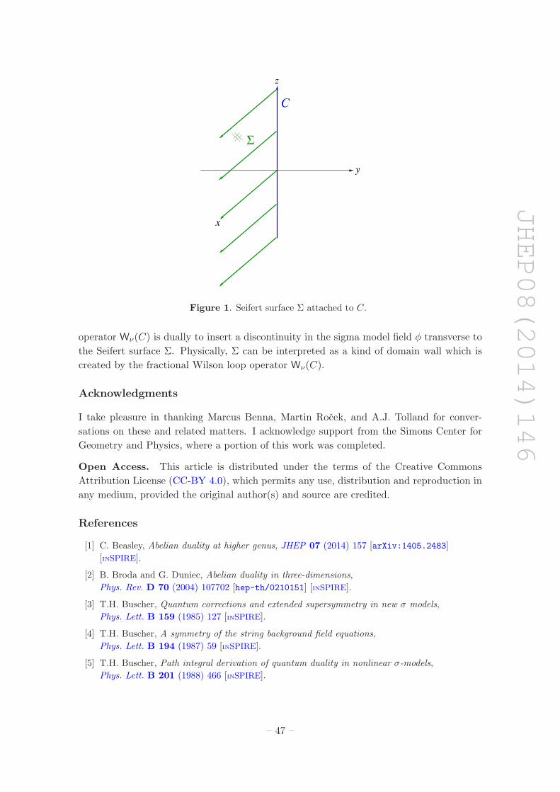
JHEP08(2014)146

Σ

x

y

z

C

Figure 1. Seifert surface Σ attached to C.

operator Wν(C) is dually to insert a discontinuity in the sigma model field φ transverse to

the Seifert surface Σ. Physically, Σ can be interpreted as a kind of domain wall which is

created by the fractional Wilson loop operator Wν(C).

Acknowledgments

I take pleasure in thanking Marcus Benna, Martin Rocek, and A.J. Tolland for conver-

sations on these and related matters. I acknowledge support from the Simons Center for

Geometry and Physics, where a portion of this work was completed.

Open Access. This article is distributed under the terms of the Creative Commons

Attribution License (CC-BY 4.0), which permits any use, distribution and reproduction in

any medium, provided the original author(s) and source are credited.

References

[1] C. Beasley, Abelian duality at higher genus, JHEP 07 (2014) 157 [arXiv:1405.2483]

[INSPIRE].

[2] B. Broda and G. Duniec, Abelian duality in three-dimensions,

Phys. Rev. D 70 (2004) 107702 [hep-th/0210151] [INSPIRE].

[3] T.H. Buscher, Quantum corrections and extended supersymmetry in new σ models,

Phys. Lett. B 159 (1985) 127 [INSPIRE].

[4] T.H. Buscher, A symmetry of the string background field equations,

Phys. Lett. B 194 (1987) 59 [INSPIRE].

[5] T.H. Buscher, Path integral derivation of quantum duality in nonlinear σ-models,

Phys. Lett. B 201 (1988) 466 [INSPIRE].

– 47 –

JHEP08(2014)146

[6] J. Cheeger, Analytic torsion and Reidemeister torsion,

Proc. Nat. Acad. Sci. USA 74 (1977) 2651.

[7] J. Cheeger, Analytic torsion and the heat equation, Ann. Math. 109 (1979) 259.

[8] S. Deser and R. Jackiw, “Self-duality” of topologically massive gauge theories,

Phys. Lett. B 139 (1984) 371 [INSPIRE].

[9] R. Dijkgraaf and E. Witten, Topological gauge theories and group cohomology,

Commun. Math. Phys. 129 (1990) 393 [INSPIRE].

[10] D. Freed, Reidemeister torsion, spectral sequences, and Brieskorn spheres,

J. Reine Angew. Math. 429 (1992) 75.

[11] T. Friedmann and E. Witten, Unification scale, proton decay and manifolds of G2 holonomy,

Adv. Theor. Math. Phys. 7 (2003) 577 [hep-th/0211269] [INSPIRE].

[12] A. Giveon, M. Porrati and E. Rabinovici, Target space duality in string theory,

Phys. Rept. 244 (1994) 77 [hep-th/9401139] [INSPIRE].

[13] P. Griffiths and J. Harris, Principles of algebraic geometry, John Wiley and Sons Inc.,

New York U.S.A. (1978).

[14] S. Gukov and E. Witten, Gauge theory, ramification, and the geometric Langlands program,

in Current developments in mathematics, D. Jerison et al. eds., Int. Press, Somerville U.S.A.

(2008), pp. 35–180 [hep-th/0612073] [INSPIRE].

[15] A. Hatcher, Algebraic topology, Cambridge University Press, Cambridge U.K. (2002).

[16] G. ’t Hooft, On the phase transition towards permanent quark confinement,

Nucl. Phys. B 138 (1978) 1 [INSPIRE].

[17] A. Karlhede, U. Lindstrom, M. Rocek and P. van Nieuwenhuizen, On 3D nonlinear

vector-vector duality, Phys. Lett. B 186 (1987) 96 [INSPIRE].

[18] A. Kapustin and M. Tikhonov, Abelian duality, walls and boundary conditions in diverse

dimensions, JHEP 11 (2009) 006 [arXiv:0904.0840] [INSPIRE].

[19] J. Milnor, Whitehead torsion, Bull. Am. Math. Soc. 72 (1966) 358.

[20] S. Minakshisundaram and A. Pleijel, Some properties of the eigenfunctions of the Laplace

operator on Riemannian manifolds, Can. J. Math. 1 (1949) 242 [INSPIRE].

[21] W. Muller, Analytic torsion and R-torsion of Riemannian manifolds,

Adv. Math. 28 (1978) 233.

[22] D. Mumford, Tata lectures on theta, I, Birkhauser, Boston U.S.A. (1983).

[23] C. Nash and D.J. O’Connor, Determinants of Laplacians, the Ray-Singer torsion on lens

spaces and the Riemann zeta function, J. Math. Phys. 36 (1995) 1462

[Erratum ibid. 36 (1995) 4549] [hep-th/9212022] [INSPIRE].

[24] L. Nicolaescu, The Reidemeister torsion of 3-manifolds, De Gruyter Studies in Mathematics,

Vol. 30, Walter De Gruyter Inc., Berlin Germany (2003).

[25] E.M. Prodanov and S. Sen, Abelian duality, Phys. Rev. D 62 (2000) 045009

[hep-th/9906143] [INSPIRE].

[26] D.B. Ray, Reidemeister torsion and the Laplacian on lens spaces, Adv. Math. 4 (1970) 109.

– 48 –

JHEP08(2014)146

[27] D.B. Ray and I.M. Singer, R-torsion and the Laplacian on Riemannian manifolds,

Adv. Math. 7 (1971) 145 [INSPIRE].

[28] M. Rocek and E.P. Verlinde, Duality, quotients and currents, Nucl. Phys. B 373 (1992) 630

[hep-th/9110053] [INSPIRE].

[29] D. Rolfsen, Knots and links, American Mathematical Society, Providence U.S.A. (1976).

[30] S. Rosenberg, The Laplacian on a Riemannian manifold: an introduction to analysis on

manifolds, London Mathematical Society Student Texts, Vol. 31, Cambridge University

Press, Cambridge U.K. (1997).

[31] P.K. Townsend, K. Pilch and P. van Nieuwenhuizen, Self-duality in odd dimensions,

Phys. Lett. B 136 (1984) 38 [Addendum ibid. B 137 (1984) 443] [INSPIRE].

[32] C. Vafa and E. Witten, A strong coupling test of S-duality, Nucl. Phys. B 431 (1994) 3

[hep-th/9408074] [INSPIRE].

[33] E.P. Verlinde, Global aspects of electric-magnetic duality, Nucl. Phys. B 455 (1995) 211

[hep-th/9506011] [INSPIRE].

[34] E. Witten, On quantum gauge theories in two dimensions,

Commun. Math. Phys. 141 (1991) 153 [INSPIRE].

[35] E. Witten, On S-duality in Abelian gauge theory, Selecta Math. 1 (1995) 383

[hep-th/9505186] [INSPIRE].

[36] E. Witten, Dynamics of quantum field theory, in Quantum fields and strings: a course for

mathematicians, Vol. 2, P. Deligne et al. eds., American Mathematical Society,

Providence U.S.A. (1999).

[37] E. Witten, SL(2,Z) action on three-dimensional conformal field theories with Abelian

symmetry, in From fields to strings: circumnavigating theoretical physics, Vol. 2,

M. Shifman et al. eds., World Scientific, Singapore (2005), pp. 1173–1200 [hep-th/0307041]

[INSPIRE].

– 49 –