GLOBAL AND REGIONAL IONOSPHERE MODELS USINGTHE GPS DOUBLE DIFFERENCE PHASE OBSERVABLE

Stefan Schaer, Gerhard Beutler, Leos Mervart, Markus RothacherAstronomical Institute, University of Berne

CH-3012 Bern, Switzerland

Urs WildFederal Office of TopographyCH-3084 Wabern, Switzerland

ABSTRACT

The CODE1 Analysis Center of the International GPS Service for Geodynamics (IGS) pro-duces orbits, Earth orientation parameters, station coordinates, and other parameters ofgeophysical interest on a daily basis using the ionosphere-free linear combination of thedouble difference phase observables. Consequently, clean (i. e. cycle-slip-free) portions ofthe L1 and the L2 phases are readily available for every day. The difference L1–L2 in meterscontains only differential ionospheric refraction effects and in the ambiguitiy-unresolvedcase a constant bias due to the initial carrier phase ambiguities in L1 and L2.Here we use exactly this observable to extract ionospheric information from the IGS net-work. On one hand it is not ideal to use the difference L1–L2 on the double difference level— the differencing reduces the ionospheric signal considerably. On the other hand we havethe advantage of a clean signal. Also, processing is simplified because satellite and receiverspecific biases cancel out to the greatest extent in our approach.As usual we model the ionospheric Total Electron Content (TEC) with a single-layer modelwhich is based on the corresponding mapping function. As opposed to earlier attempts (localionosphere models using Taylor series expansions in latitude and sun-fixed longitude) wedevelop the vertical TEC into a series of spherical harmonics. We may use the geocentriclatitude and the sun-fixed longitude or an equivalent set in the solar-geomagnetic system asindependent arguments. These models have the advantage — over Taylor series expansions— to be well suited for regional and for global models.First results using one week of regional (European) and global data (entire IGS network)from the CODE Analysis Center seem to indicate that under normal ionospheric condi-tions the ionosphere models are very useful for single-frequency GPS users, i. e. ionosphericrefraction effects are greatly reduced if these TEC models are taken into account.

1Center for Orbit Determination in Europe

Paper presented at the 1995 IGS Workshop, Potsdam, Germany, May 15–17, 1995

INTRODUCTION

Ionospheric refraction was considered as an important aspect within the GPS group of theAstronomical Institute of the University of Berne (AIUB) for a long time. In the time periodwhen usually only single-band (L1) receivers were available it was important to get insightinto the biases introduced in a GPS network by unmodeled ionospheric refraction (Beutler etal., 1988). Later on, it became obvious that short period variations in ionospheric refractioncould harm GPS analyses even if dual-band receivers were available (Beutler et al., 1989).In the latter paper there were also clues that valuable information about the ionospherecould be extracted from dual-band GPS data.

Modeling and monitoring the ionosphere was the main topic of the Ph.D. thesis (Wild,1994). In this thesis it could be shown that local ionosphere models like those presentedby (Georgiadiou and Kleusberg, 1988) are very efficient to remove — or greatly reduce —the scale bias for single-band receivers operating in the vicinity of dual-band receivers, thedata of which were used to establish a local ionosphere model. (Wild, 1994) computed suchlocal ionosphere models for a number of IGS sites over an extended time period. He alsodescribes a procedure to assess the stochastic behaviour of the ionosphere in the vicinityof a GPS station. The principal conclusion was that essential information concerning theionosphere might be extracted from the IGS network. Local ionosphere models have provedtheir usefulness on many occasions. However, the concept of having as many ionospheremodels as stations in a network like that of the IGS is hardly operational. The modelingtechniques used by (Wild, 1994) had to be modified in one important respect before itbecame possible to replace N local models by one regional or global model based on thedata of N stations.

Let us briefly review the modeling features as used by (Wild, 1994) and as used below.Wild uses the so-called single-layer model where it is assumed that all free electrons areconcentrated in a shell of infinitesimal thickness. This thin shell is located in a height H

above a spherical Earth. The height H of this idealized layer is usually set to 350 or 400 kilo-meters, which corresponds approximately to the peak height of the electron density profilein the F-region of the ionosphere. The electron density E — the surface density of the layer— is assumed to be a function of the geocentric latitude β and the sun-fixed longitude s

E(β, s) =n∑

i=0

m∑

j=0

Eij · (β − β0)i · (s− s0)

j (1)

where

n,m are the maximum degrees of the two-dimensional Taylor series expansion inlatitude and in sun-fixed longitude,

Eij are the (unknown) coefficients of the Taylor series, and

β0, s0 are the coordinates of the origin of the development.

The single-layer model defined by equation (1) does not provide a modeling of the timedependence in the sun-fixed reference frame because the “frozen” ionosphere is co-rotatingwith the Sun. Nevertheless, there is always a time dependence in the earth-fixed frame. Note

2

that short-term variations of the ionospheric TEC are not modeled by equation (1). Theywill be interpreted as noise of the geometry-free GPS observable.

The representation (1) is not well suited for regional or global TEC models because oflimitations in the (β, s)-space. Based on the above considerations we decided to use a newapproach to model the ionosphere in the following way (details explained in the next section):

(i) The single-layer model is used as previously.

(ii) The mapping function is taken over without change.

(iii) The zero-difference observable was replaced by the double-difference observable dueto operational considerations.

(iv) Instead of using a Taylor series development a development into spherical harmonicswas used.

As already mentioned above we are fully aware of the fact that by using double insteadof zero differences we lose parts of the ionospheric signal but we have the advantage of acleaned observable. Moreover we are not affected by a degradation of the code observationsunder the AS-regime. This advantage may be “lost” when the next generation of preciseP-code receivers will become available.

THE “NEW” IONOSPHERE MODELING TECHNIQUE

The double-differenced observation equation for the geometry-free linear combination φ4 ofthe carrier phase measurements (φ1 and φ2) referring to a set of two receivers and twosatellites may be written as

dd(φ4) + v4 = −α

(1

ν21

−1

ν22

)dd(F (z) · E) +B4 (2)

where

dd(. . .) is the double-difference operator ,

φ4 = φ1 − φ2 is the geometry-free phase observable (in meters),

v4 is the corresponding residual,

α = 4.03 · 1017 ms−2 TECU−1 is a constant (TECU stands for Total Electron ContentUnit2),

ν1, ν2 are the frequencies associated with the carriers L1 and L2,

F (z) is the mapping function evaluated at the zenith distance z,

E is the vertical Total Electron Content (in TECU), and

2One TEC Unit corresponds to 1016 free electrons per square meter.

3

B4 = λ1 N1 − λ2 N2 is a constant bias (in meters) due to the initial phase ambiguities N1

and N2 with their corresponding wavelengths λ1 and λ2; if new ambiguitieswere set up for one satellite, a new parameter of this type has to be introduced.

In the ambiguity-resolved case the (integer) double-difference ambiguity parameters N1 andN2 as well as the (real-valued) parameter B4 are known. All unresolved ambiguity para-meters B4 — auxiliary parameters only — and the ionosphere model parameters have tobe estimated simultaneously.

The single-layer or thin-shell mapping function F (z) simply may be written as

F (z) =1

cos z′=

1√1− sin2 z′

with sin z′ =R

R+Hsin z (3)

where

z, z′ are the (geocentric) zenith distances at the station and at the single layer,

R is the mean Earth radius, and

H is the height of the single layer above the Earth’s surface.

We develop the surface density E of the ionospheric layer into a series of spherical harmonicfunctions of maximum degree nmax and maximum order mmax ≤ nmax:

E(β, s) =nmax∑

n=0

n∑

m=0

Pnm(sin β) · (anm cosms+ bnm sinms) with t ∈ [ti, ti+1] (4)

where

β is the geocentric latitude of the intersection point of the line receiver–satellitewith the ionospheric layer,

s = λ− λ0 is the sun-fixed longitude of the ionospheric pierce point, which correspondsto the local solar time neglecting an additive constant π (or 12 hours),

λ, λ0 are the geographic longitude of the ionospheric pierce point and the true (ormean) longitude of the Sun,

t is the time argument,

[ti, ti+1] is the specified period of validity (of the i-th model),

Pnm = Λ(n,m) · Pnm are the normalized associated Legendre polynomials of degree n

and order m based on the normalization function Λ and the unnormalizedLegendre polynomials Pnm, and

anm, bnm are the unknown coefficients of the spherical harmonic functions, i. e. the global(or regional) ionosphere model parameters.

We may use the geocentric latitude β and the sun-fixed longitude s in the geographicalcoordinate system or an equivalent set (β′, s′) in the solar-geomagnetic coordinate system

4

as independent arguments. Using simply the mean longitude of the Sun, the sun-fixed meanlongitude s of the ionospheric pierce point in the geographical system reads as

s = λ− λ0 = λ− (π − t) = λ+ t− π (5)

where t is the Universal Time UT (in radians).

The normalization function Λ is defined as follows:

Λ(n,m) =

√

22n+ 1

1 + δ0m

(n−m)!

(n+m)!with Λ(0, 0) = 1 (6)

where δ denotes the Kronecker Delta.

The zero-degree coefficient a00 may be interpreted on a global scale as the mean TEC E0

by forming the surface integral of the TEC distribution (4)

E0 =1

4π

∫

S

E dS =1

4π

∫ +π

2

−π

2

∫ 2π

0

E(β, s) cos β dβ ds = Λ(0, 0) a00 = a00 (7)

Multiplying the coefficient a00 (in TECU) by the surface area of the ionospheric layer (inm2) we obtain the total number of free electrons nE (in 1016) within the ionospheric shell

nE = 4π R′2 a00 with R′ = R+H (8)

where R′ is the geocentric radius of the ionospheric layer.

The number nP of ionosphere model parameters anm and bnm (per parameter set) is givenby the expression

nP = (nmax + 1)2 − (nmax −mmax) (nmax −mmax + 1) with mmax ≤ nmax (9)

or by

nP = (nmax + 1)2 if nmax = mmax (10)

Both TEC models (1) and (4) represent a static (or “frozen”) ionosphere in the sun-fixedreference frame. However, the parametrization of the ionospheric coefficients anm and bnmas time-dependent parameters — for instance as piece-wise linear functions in time ensuringthe continuity — allow us theoretically to model a (low-)dynamic ionosphere E(β, s, t). Insummary, we are able to set up in our procedure a set of constant ionosphere parametersper specified time interval [ti, ti+1] or a parameter set per specified reference epoch ti whilethe ionosphere coefficients anm(t) and bnm(t) are interpolated linearly in time between sub-sequent epochs ti. This modeling technique was not followed up in detail. Attempts weremade specifying each 24 hours reference epochs ti to generate a sequence of quasi-staticionosphere models continuously varying in time.

5

The global ionosphere model parameter type as presented here has been implementedinto the parameter estimation program GPSEST of the Bernese GPS Software, where theparameter estimation algorithm is based on a least-squares adjustment.

FIRST RESULTS

At present (mid 1995), the CODE Analysis Center is processing the data of about 60globally distributed sites of the GPS tracking network of the IGS. Figure 1 shows the presentstate of the IGS core network. Notice in particular the station distribution in latitude withNyAlesund as the IGS station furthest north (78.9 N) and McMurdo as the station furthestsouth (77.8 S).

Albert HeadAlgonquin

Arequipa

Bermuda

Fairbanks

Fortaleza

Hartebeesthoek

Kokee Park

Kourou

Maspalomas

Matera

McDonald

Metsahovi

North Liberty

Ny Ålesund

Onsala

Pamatai

Penticton

Perth

Pie Town

Richmond

Santiago

Tromsø

Yellowknife

CaseyDavis

St. John'sWestford

Bogotá

Kitab

Potsdam

Kerguélen

Wettzell

Zwenigorod

O' Higgins

060 12060

Brasília

Thule

Lhasa

Madrid

La Plata

Kellyville

Easter Island

Greenbelt

Bangalore

Kiruna

SOUTHERNCALIFORNIA

INTEGRATEDGPS NETWORKS

(29 SITES)

St. Croix

Reykjavík

Bishkek

Irkutsk

Seychelles Malindi

Ankara

Noto

Padova

Mendeleevo

Catalonia

Grasse

HerstmonceuxBrussels

Zimmerwald

KootwijkBorowiec

Jozefoslaw

QuincyMammoth

San Fernando

Graz

Villafranca

Goldstone

Figure 1. GPS tracking network of the International GPS Service for Geodynamics (IGS)— operational and planned stations (May 1995)

Looking at Figure 1 the inhomogeneous distribution of the IGS sites and even the sparsecoverage in the southern hemisphere can be clearly seen. Obviously, a high-temporal re-solution of the TEC structure without any gaps over the entire globe will not be possible,because each GPS station “observes” the ionosphere within a radius of 1 000 (1 500) kilo-meters only when using an elevation angle cutoff at 20 (15) .

6

Global Ionosphere Models

Below we discuss results using a data set of April 23–29, 1995 (GPS week 798, DOY 113–119). Let us summarize some important aspects first. For all subsequent computations, asingle-layer height H of 400 kilometers is assumed. Furthermore all ionosphere models (ormaps) are derived from double-differenced GPS phase data using an elevation angle cutoff at20 — as used for our routine processing — and a sampling rate of one epoch per 4 minutes3.

An 8th-degree spherical harmonics expansion (4) is normally performed for a 24-hourglobal ionosphere model . Consequently, this 24-hour model represents a time-averaged TECstructure, which is a static (or “frozen”) one in the sun-fixed reference frame. According toformula (10) the number of ionosphere parameters per such a TEC model is 81.

In order to illustrate ionosphere maps, the results for April 23, 1995 are included in thispaper. Figure 2 shows the global ionosphere map based on the geographical coordinate sys-tem in the ambiguity-free and ambiguity-fixed case respectively. In both cases the maximumTEC is about 47 TECU (explicitly plotted in Figures 4a and 4b). The sun-fixed longitudes sof the ionospheric pierce points have been computed according to the simplified relation (5)as mean longitudes. In Figure 2 (and 3) the latitude band of the ionospheric pierce pointsis indicated by the two dashed lines.

−150 −100 −50 0 50 100 150

−80

−60

−40

−20

0

20

40

60

80

0

5

5

5

10 10

15

20 25

30

35

40 45

Total Electron Content (TEC Units), day 113 of year 1995, A

Sun−fixed mean longitude (degrees)

Geo

grap

hic

latit

ude

(deg

rees

)

(a) Ambiguity-free solution

−150 −100 −50 0 50 100 150

−80

−60

−40

−20

0

20

40

60

80

0

0

5

5

10

10

15 20

25

30 35

40

45

Total Electron Content (TEC Units), day 113 of year 1995, B

Sun−fixed mean longitude (degrees)

Geo

grap

hic

latit

ude

(deg

rees

)

(b) Ambiguity-fixed solution

Figure 2. Global ionosphere map for April 23, 1995 based on the geographical coordinatesystem (with 81 coefficients, i. e. nmax = mmax = 8 )

On day 113 about 48% of roughly 2 200 ambiguity parameters B4 (see observation equa-tion (2)) were resolved (i. e. known). Ambiguity resolution4 without using the P-code meas-urements is performed up to baseline lengths of 2 000 kilometers (Mervart, 1995); where

3One epoch per 30 seconds would be available.4We use the so-called Quasi-Ionosphere-Free (QIF) ambiguity resolution strategy.

7

typically about 85 (90)% of the ambiguities are resolved for baseline lengths l < 500 km,80 (85)% for l < 1 000 km, and 70 (75)% for l < 2 000 km when Anti-Spoofing (AS) is turnedon (off). By resolving the ambiguities we achieve primarily a drastic reduction of the numberof unknown parameters as well as an improvement in accuracy of the remaining parameters.Since June 25, 1995 (GPS week 807, DOY 176) — after an experimental phase of severalmonths — the official IGS products from the CODE Analysis Center are based on (partly)ambiguity-fixed solutions.

To study the effect of choosing the geographical and the solar-geomagnetic coordinatesystem respectively, we have compared global ionosphere models based on each coordinatesystem for all days of GPS week 798. However, we could not recognize any significantdifference in terms of the root-mean-square (RMS) error of the unit weight. Figure 3 showsthe ionosphere map for April 23, 1995 based on the solar-geomagnetic coordinate system inthe ambiguity-fixed case.

−150 −100 −50 0 50 100 150

−80

−60

−40

−20

0

20

40

60

80

0

0

5

5 5

5

5

10

10

15 15

15

20

25 30

35 40

45

Total Electron Content (TEC Units), day 113 of year 1995, B

Sun−fixed longitude (degrees)

Geo

mag

netic

latit

ude

(deg

rees

)

Figure 3. Global ionosphere map for April 23, 1995 based on the solar-geomagnetic co-ordinate system (with 81 coefficients, i. e. nmax = mmax = 8)

Comparing Figure 3 with Figure 2b both contour line maps look similar. Note that thegeomagnetic latitude of the Sun varies considerably (ca. ±10.9 ) as opposed to the geo-

8

graphical system, where the latitude of the Sun remains nearly constant over the time spanof 24 hours.5

The development in time of three special quantities namely the maximum, mean, and“minimum” TEC is shown in Figure 4. The values coming from solutions based on boththe geographical and the geomagnetic frame are very similar, hence the values of the firstset only are plotted.

113 114 115 116 117 118 119 120

0

10

20

30

40

50

DOY

Max

imum

, mea

n, a

nd m

inim

um T

EC

(T

EC

U)

GPS week 798, A

(a) Ambiguity-free solutions

113 114 115 116 117 118 119 120

0

10

20

30

40

50

DOY

Max

imum

, mea

n, a

nd m

inim

um T

EC

(T

EC

U)

GPS week 798, B

(b) Ambiguity-fixed solutions

Figure 4. Development in time of the daily maximum, mean, and “minimum” TECs duringGPS week 798

According to the surface integral (7) the mean TEC E0 is represented by the zero-degreecoefficient a00. Using the simple relation (8) we can convert a00 (or E0) into the totalnumber nE of free electrons within the ionospheric shell: e. g. nE = 6.5 ·1031 at day 113. Themean TEC (or the time-averaged total number of free electrons) steadily decreasing duringGPS week 798 (see Figure 4) seems to be quite stable (small variations). After fitting the“observed” ionospheric coefficients a00 by a first-degree polynomial in time, we have gotresiduals with an RMS error of 0.3 TECU, which is a first criterion for the quality of thespecial ionosphere parameter a00 (or E0). Theoretically the quantity E0 should be a goodindicator for the solar activity. One may expect that this ionospheric parameter is stronglycorrelated with the Sun spot number . We should mention that the solar activity was quiteweak (low Sun spot number) during this test week.

By definition the TEC must be greater than zero. Accordingly, the “minimum” TECestimates are never significantly below zero, which is a sign of success, too (we have neverapplied any a priori constraints on the ionosphere model parameters).

5The current geographic latitude of the geomagnetic pole is about 79.1 .

9

Regional Ionosphere Models

When processing data from tracking stations located within a narrow longitude band, theionosphere modeling technique (4) yields regional ionosphere models. An example of aregional ionosphere map is shown in Figure 5a compared with the corresponding detail(latitude band) of the global TEC map (see Figures 2b and 5b). Both maps are based onambiguity-fixed GPS solutions using the geographical coordinate system.

−150 −100 −50 0 50 100 15035

40

45

50

55

60

65

70

2.5

2.5

2.5

2.5

5

7.5

10

12.5

15

Total Electron Content (TEC Units), day 113 of year 1995, B

Sun−fixed mean longitude (degrees)

Geo

grap

hic

latit

ude

(deg

rees

)

(a) Regional TEC map (for Europe)

−150 −100 −50 0 50 100 15035

40

45

50

55

60

65

70

2.5

2.5

5

5

7.5

10

12.5

Total Electron Content (TEC Units), day 113 of year 1995, B

Sun−fixed mean longitude (degrees)

Geo

grap

hic

latit

ude

(deg

rees

)

(b) Global TEC map (detail only)

Figure 5. The regional TEC model (with nmax = 5) for April 23, 1995 is based on dataof 16 European IGS stations (listed in Tables 1 and 2), whereas the global TECmodel (with nmax = 10) is based on data of 50 globally distributed IGS stations(including the European ones).

The TEC model (4) — its specified period of validity assumed to be not longer than24 hours (i. e. ti+1 − ti ≤ 24 h) — provides for a regional model a real modeling of thetime dependence in the sun-fixed reference frame because by definition the longitude band[λmin, λmax] of the monitor stations is small, i. e.

λmax − λmin ≪ 2π (11)

Therefore the monitor stations of a regional network “probe” at every time only a narrowlongitude band of the ionosphere co-rotating with the Sun. A restriction of the latitude bandwould not be necessary, but is given by the station geometry. Considering these restrictionsthe regional ionosphere model (Figure 5a) is applicable only for GPS stations lying withinthe latitude band [40 N, 70 N] and strictly speaking within the “narrow” longitude band[4 W, 37 E], as opposed to the global model (Figure 5b), where we assume the TEC tobe longitude-independent. Notice that Figure 5a shows the (wider) latitude band of theionospheric pierce points.

10

The special case of processing individual baselines (two stations) only to generate so-called baseline-specific ionosphere models was already considered in (Schaer, 1994). Thefollowing Figures 6a, 6b, and 7b (from (Schaer, 1994)) are based on results of L1-L2-solutionscontaining station coordinates, ambiguities (N1 and N2), tropospheric zenith path delayparameters, stochastic ionosphere parameters, and last but not least deterministic iono-sphere parameters according to TEC model (4) with H = 350 km. Figure 6 illustrates thebaseline-specific ionosphere model for the baseline Kootwijk–Wettzell (Europe) before andafter ambiguity resolution respectively. The “bulge” at (local) early afternoon as well as agradient in north-south direction are clearly recognizable. The ionospheric activity at thattime seems to have been much stronger than 15 months later as seen in the TEC map forEurope (Figure 5a).

42

44

46

48

50

52

54

56

0 5 10 15 20

+0

+0

+0

+2.5

+2.5

+5

+5

+7.5

+7.5

+10

+10+12.5

+12.5

+15

+15

+17.5

+17.5

+20

+22.5

Total Electron Content in [TECU] before ambiguity resolution

Local time in [hours]

Lat

itude

in [

degr

ees]

(a) Before ambiguity resolution

42

44

46

48

50

52

54

56

0 5 10 15 20

+0

+2.5

+2.5

+2.5

+2.5

+5

+5

+5

+7.5

+7.5

+10 +10+12.5

+12.5

+15

+17.5

+20

Total Electron Content in [TECU] after ambiguity resolution

Local time in [hours]

Lat

itude

in [

degr

ees]

(b) After ambiguity resolution

Figure 6. Baseline-specific ionosphere model with 36 parameters (nmax = 5) for baselineKootwijk–Wettzell (l ≈ 600 km) at January 25, 1994

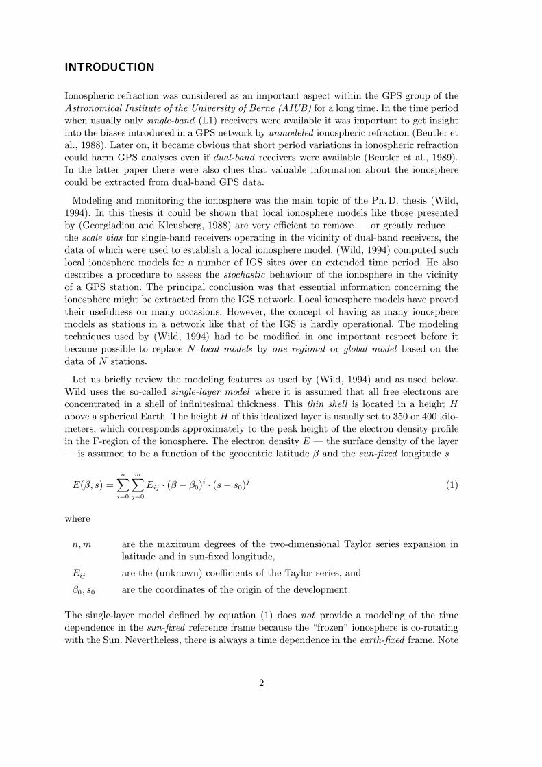
The fractional parts of the wide-lane ambiguities N5 = N1 − N2 just before fixing areshown in Figure 7b. Note that our “fractional parts” are not generally the differences withrespect to the next integer but the differences between true and biased ambiguity para-meters; therefore they may be greater than half a cycle (see Figure 7a). Assuming that thestation coordinates and the troposphere parameters (or the “geometrical” parameters) arewell determined, these fractional parts are proportional to the biases due to the ionosphericrefraction.6 The dispersion of the fractional parts of the ambiguities N5 is consequentlyan excellent indicator for the unmodeled ionospheric influence or the quality of the iono-sphere modeling of course — at least on differential level. Comparing Figures 7a and 7b thedecreasing of this dispersion when TEC is modeled is clearly visible.

6One wide-lane cycle (λ5 = 86 cm) corresponds approximately to 4.1 TECU (at z = 0).

11

0

5

10

15

20

-1 -0.8 -0.6 -0.4 -0.2 0 0.2 0.4 0.6 0.8 1

No deterministic ionosphere model estimated

Fractional part of wide-lane ambiguity in [cycles]

Num

ber

of w

ide-

lane

am

bigu

ities

(a) Without TEC modeling

0

5

10

15

20

-1 -0.8 -0.6 -0.4 -0.2 0 0.2 0.4 0.6 0.8 1

Baseline-specific ionosphere model estimated

Fractional part of wide-lane ambiguity in [cycles]

Num

ber

of w

ide-

lane

am

bigu

ities

(b) With TEC modeling

Figure 7. Histogram of the fractional parts of the wide-lane ambiguities for one-day single-baseline solution — without or with TEC modeling (Figure 6a)

Quality Checks

Applying the ionosphere model (4) the ionospheric range correction (in meters) for thezero-difference GPS observation of the i-th frequency is given by

∆i(β, s, z) = ∓α

ν2i

F (z) ·E(β, s) with i = 1, 2 (12)

where one has to select the negative sign for phase observations and the positive for codeobservations (see also equations (2) and (3)). It is very important to use in relation (12) thesame height H of the single layer the TEC model (4) is based on, whereas GPS results arenearly insensitive to the value itself of the height H (Wild, 1994). Nevertheless, the absolutecalibration of the TEC E strongly depends on the assumed height H of the single layer.

In order to get a first impression of the quality of our large-scale ionosphere models we com-puted regional single-frequency (L1) solutions with European data with and without regionaland global ionosphere models respectively applied according to the above formula (12). Notethat the maximum extent of this IGS sub-network evaluated is about 3 500 kilometers indiameter. The baseline shortening introduced into GPS results by neglecting the ionosphericrefraction is on the average 0.08 ppm/TECU when the L1 phase observable is processed withan elevation mask at 20 (Beutler et al., 1988). We expect an apparent network contractionof the same order.

Analyzing the scale biases estimated and the residuals of the coordinates coming fromHelmert transformations with respect to ITRF7 coordinates, we observed for every day of

7IERS (International Earth Rotation Service) Terrestrial Reference Frame

12

the test week that when applying our ionosphere models not only the scale bias has beenreliably removed (on the 10-ppb level) but also the RMS variance of the residuals could bereduced significantly. No perceptible quality difference between regional and global iono-sphere models could be detected by these criteria. Results of the seven parameter Helmerttransformation between ITRF coordinates and the station coordinates of the regional single-frequency solution for the first day of the test week are shown in Table 1. The scale biasestimated is given at the bottom of the table: −0.25 ppm (without) and −0.02 ppm (withTEC model). The global TEC model illustrated in Figure 2b was used. The statistics of thecorresponding six parameter Helmert transformation (no scale bias estimated) is given inTable 2. A dramatic increase of the standard deviation of the station coordinates when noTEC model is used has to be expected.

Table 1. Seven parameter Helmert transformation between ITRF coordinates and the co-ordinates of the regional L1 solution processing European IGS data from April 23,1995

Global TEC model applied No Yes

Station name Residuals (cm) Residuals (cm)North East Up North East Up

JOZE Jozefoslaw 2.1 −0.4 6.6 1.8 −3.7 4.4BRUS Brussels −4.6 −4.5 9.2 −2.7 −2.8 3.2BOR1 Borowiec 1.0 0.7 7.3 1.0 −1.2 3.3GRAZ Graz 4.9 1.4 −3.3 4.6 −1.8 −4.1HERS Herstmonceux −6.7 −3.4 −1.4 −5.4 −0.7 −1.5KOSG Kootwijk 0.5 −4.4 9.2 0.3 −3.6 5.6MADR Madrid 12.8 2.7 −9.8 15.2 8.8 −4.5MATE Matera 2.2 10.0 −19.6 1.1 4.3 −5.0TROM Tromso 2.4 11.3 −24.5 −2.0 13.4 −13.0WETT Wettzell 3.3 −1.9 7.2 3.2 −3.4 3.4ZIMM Zimmerwald −8.4 −2.2 −6.7 −7.2 −1.6 −9.1ONSA Onsala −8.1 0.4 13.7 −7.8 2.0 12.1METS Metsahovi −3.3 1.0 −6.3 −2.9 4.2 −4.4POTS Potsdam 1.4 −0.9 7.1 0.8 −1.2 3.1LAMA Lamkowko −1.7 1.9 10.8 −1.8 −0.7 6.8MDVO Mendeleevo 2.4 −11.7 0.6 1.7 −12.1 −0.3RMS per component (cm) 5.4 5.4 11.1 5.4 5.8 6.4RMS of transformation (cm) 8.2 6.2Degree of freedom 41 41Scale factor (mm/km) −0.252± 0.020 −0.018± 0.015

This method to perform quality checks indicates GPS-internal consistency of the ionospheremodels. The same is true for the analysis of the fractional parts of wide-lane ambiguityparameters (Figure 7b). In order to check the absolute calibration of our TEC models,comparisons with models established by other groups using other techniques or even otherthan GPS observations will have to be made.

13

Table 2. Six parameter Helmert transformation (no scale factor permitted) between ITRFcoordinates and the coordinates of the regional L1 solution processing EuropeanIGS data from April 23, 1995

Global TEC model applied No Yes

Station name Residuals (cm) Residuals (cm)North East Up North East Up

JOZE Jozefoslaw 2.2 13.0 5.1 1.8 −2.7 4.3BRUS Brussels −1.1 −20.2 8.0 −2.4 −3.9 3.1BOR1 Borowiec 1.2 7.3 5.4 1.0 −0.7 3.2GRAZ Graz 19.7 5.7 −4.5 5.6 −1.5 −4.1HERS Herstmonceux −4.5 −26.1 −1.8 −5.2 −2.3 −1.5KOSG Kootwijk 0.4 −17.1 7.7 0.3 −4.5 5.5MADR Madrid 41.6 −34.1 −4.9 17.3 6.2 −4.2MATE Matera 34.7 17.4 −18.2 3.4 4.9 −4.9TROM Tromso −45.6 16.9 −19.1 −5.4 13.8 −12.6WETT Wettzell 12.4 −2.5 5.4 3.9 −3.4 3.2ZIMM Zimmerwald 6.6 −13.2 −7.6 −6.1 −2.4 −9.2ONSA Onsala −22.2 −1.6 12.3 −8.8 1.8 12.0METS Metsahovi −26.4 16.5 −5.9 −4.6 5.3 −4.4POTS Potsdam 1.4 −1.1 5.0 0.8 −1.3 3.0LAMA Lamkowko −6.5 14.2 9.4 −2.2 0.2 6.7MDVO Mendeleevo −13.9 24.9 3.7 0.5 −9.5 −0.1RMS per component (cm) 21.7 17.6 9.4 6.1 5.4 6.3RMS of transformation (cm) 17.6 6.2Degree of freedom 42 42

CONCLUSIONS AND OUTLOOK

The world-wide IGS network of permanent tracking dual-frequency GPS receivers providesa unique opportunity to continuously monitor the Total Electron Content (TEC) on a globalscale. First results using one week of GPS phase data as used by the CODE Analysis Centerseem to indicate that under normal ionospheric conditions we are able to estimate plausibleionosphere models using the double-difference approach. Results were illustrated by severalionosphere maps for April 23, 1995.

An 8th-degree spherical harmonics expansion seems to be adequate for a 24-hour globalTEC model. This 24-hour model represents a time-averaged global TEC structure. To verifythe GPS-internal consistency of our TEC models we computed regional single-frequency(L1) solutions with European data with and without using regional and global models, re-spectively. Comparisons by Helmert transformations between the station coordinates stem-ming from the different L1 solutions and the corresponding ITRF coordinates revealed thatwhen applying our ionosphere models not only the scale biases could be reliably removed, asignificant reduction of the residuals could be observed as well for every day of the test week.No quality difference between regional and global ionosphere models could be detected. Inorder to check in detail the quality as well as the absolute calibration of our TEC models,comparisons with models established by other groups will have to be made.

14

The assumptions of the thin-shell model — the height H of the shell in particular — areessential for absolute calibration. If a smaller (larger) height than the “effective” (or actual)height H0 is adopted, larger (smaller) zenith distances at the ionospheric sub-points willcause the TEC values to be underestimated (overestimated). This means that in principlethe determination of the single-layer height H as an additional unknown parameter wouldbe possible.

The use of the double-difference approach will give us the capability to produce very “low-cost” one-day ionosphere models (and maps) on a routine basis — even under Anti-Spoofing(AS). The ionosphere modeling technique presented in this paper will be implemented atthe CODE Analysis Center in the very near future. An additional fully-automatic procedurewill be set up to create ionosphere model files for every day. These daily average ionospheremodels should potentially support our so-called Quasi-Ionosphere-Free (QIF) ambiguityresolution strategy (Mervart and Schaer, 1994). By statistically analyzing the fractionalparts of the wide-lane ambiguities we will get another quality check indicator for our iono-sphere models. After ambiguity resolution we will be able to generate ionosphere modelswhich are based on (partly) ambiguity-fixed solutions.

The ionosphere model parameters (global ionosphere maps only) will not be sent to theIGS Global Data Centers, but will be made available in an Anonymous FTP account at theCODE processing center.8 Such an ionosphere service providing day by day TEC modelsis of interest for all GPS users, which are analyzing and evaluating small high-precisioncontrol networks using the L1 observable only instead of the ionosphere-free LC for reasonsof accuracy (see e. g. (Beutler et al., 1995)). Finally, let us not forget that we will obtaininformation related to the ionosphere (and the solar activity) like mean TEC, maximumTEC, etc. for long-term studies.

REFERENCES

Beutler, G., I. Bauersima, W. Gurtner, M. Rothacher, T. Schildknecht, 1988, AtmosphericRefraction and Other Important Biases in GPS Carrier Phase Observations, Mono-graph 12, School of Surveying, University of New South Wales, Australia.

Beutler, G., I. Bauersima, S. Botton, W. Gurtner, M. Rothacher, T. Schildknecht, 1989,Accuracy and biases in the geodetic application of the Global Positioning System,Manuscripta Geodaetica, Vol. 14, No. 1, pp. 28–35.

Beutler, G., I. I. Mueller, R. Neilan, 1994, The International GPS Service for Geo-dynamics (IGS): Development and Start of Official Service on 1 January 1994, BulletinGeodesique, Vol. 68, No. 1, pp. 43–51.

Beutler, G., M. Cocard, A. Geiger, M. Muller, M. Rothacher, S. Schaer, D. Schneider,A. Wiget, 1995, Dreidimensionales Testnetz Turtmann 1985–1993: Teil II, Geodatisch-geophysikalische Arbeiten in der Schweiz , Band 51.

Georgiadiou, Y. and A. Kleusberg, 1988, On the effect of ionospheric delay on geodeticrelative GPS positioning, Manuscripta Geodaetica, Vol. 13, pp. 1–8.

8The next version of the Bernese GPS Software will be able to process directly these ionosphere files.

15

Lanyi, G. E. and T. Roth, 1988, A comparison of mapped and measured total ionosphericelectron content using global positioning system and beacon satellite observations,Radio Science, Vol. 23, No. 4, pp. 483–492.

Mannucci, A. J., B.D. Wilson, D.-N. Yuan, 1994, Monitoring Ionospheric Total ElectronContent Using the GPS Global Network and TOPEX/POSEIDON Altimeter Data,Proceedings of the Beacon Satellite Symposium, Aberystwyth, Wales, July 1994.

Mervart, L., G. Beutler, M. Rothacher, U. Wild, 1993, Ambiguity Resolution StrategiesUsing the Results of the International GPS Geodynamics Service (IGS), BulletinGeodesique, Vol. 68, No. 1, pp. 29–38.

Mervart, L. and S. Schaer, 1994, Quasi-Ionosphere-Free (QIF) Ambiguity ResolutionStrategy, Internal report, Astronomical Institute, University of Berne, Switzerland.

Mervart, L., 1995, Ambiguity Resolution Techniques in Geodetic and GeodynamicApplications of the Global Positioning System, Ph.D. thesis, Astronomical Institute,University of Berne, Switzerland.

Rothacher, M., G. Beutler, W. Gurtner, E. Brockmann, L. Mervart, 1993, The BerneseGPS Software Version 3.4: Documentation, Astronomical Institute, University ofBerne, Switzerland.

Rothacher, M., R. Weber, E. Brockmann, G. Beutler, L. Mervart, U. Wild, A. Wiget,C. Boucher, S. Botton, H. Seeger, 1994, Annual Report 1994 of the CODE ProcessingCenter of the IGS .

Schaer, S., 1994, Stochastische Ionospharenmodellierung beim Rapid Static Positioning mitGPS , Diplomarbeit, Astronomisches Institut, Universitat Bern.

Wild, U., 1993, Ionosphere and Ambiguity Resolution, Proceedings of the 1993 IGS Work-shop, March 25–26, 1993, Berne, Switzerland, pp. 361–369.

Wild, U., 1994, Ionosphere and Satellite Systems: Permanent GPS Tracking Data forModelling and Monitoring, Geodatisch-geophysikalische Arbeiten in der Schweiz ,Band 48.

Wilson, B.D. and A. J. Mannucci, 1993, Instrumental Biases in Ionospheric measurementsDerived from GPS Data, Paper presented at ION GPS 93, Salt Like City, September22–24, 1993.

16