global and local cardiac functional analysis with cine mr

Global and Local Cardiac Functional Analysis with Cine MR Imaging: A

Non-Rigid Image Registration Approach

Except where reference is made to the work of others, the work described in thisdissertation is my own or was done in collaboration with my advisory committee. This

dissertation does not include proprietary or classified information.

Wei Feng

Certificate of Approval:

Stanley J. ReevesProfessorElectrical and Computer Engineering

Thomas S. Denney Jr.ProfessorElectrical and Computer Engineering

Jitendra K. TugnaitJames B. Davis ProfessorElectrical and Computer Engineering

George T. FlowersDeanGraduate School



Wei Feng

A Dissertation

Submitted to

the Graduate Faculty of

Auburn University

in Partial Fulfillment of the

Requirements for the

Degree of

Doctor of Philosophy

Auburn, AlabamaAugust 10, 2009



Wei Feng

Permission is granted to Auburn University to make copies of this dissertation at itsdiscretion, upon the request of individuals or institutions and at

their expense. The author reserves all publication rights.

Signature of Author

Date of Graduation

iii

Vita

Wei Feng, only son and the third child of Zhiguo Feng and Shulan He, was born in

Tangshan city, Hebei Province, China on Nov. 28, 1976. He graduated from the First High

School of Luanxian in 1996 and was enrolled in Shanghai Jiao Tong University the same

year, where he earned both his Bachelor of Engineering and Master of Science degrees in

electrical engineering in 2000 and 2003, respectively. He then worked for Magima Inc. in

2003 for several months before he went to the United States with his beloved wife, Shuang

Feng. He then entered the PhD program in electrical engineering of Auburn University in

Aug. 2004, where he is expected to acquire the degree in Aug. 2009. He was accepted

in the Master’s program in mathematics of Auburn University in Feb. 2008. He and his

wife shared the same high school, the same university for their undergraduate and graduate

years in China, and the same university in the United States in Auburn. They are blessed

with a lovely daughter, Grace T. Feng, who was born on May 19, 2005.

iv

Dissertation Abstract



Wei Feng

Doctor of Philosophy, August 10, 2009(M.S. (Mathematics), Auburn University, 2008)

(M.E. (Electrical Engineering), Shanghai Jiao Tong University, 2003)(B.S. (Electrical Engineering), Shanghai Jiao Tong University, 2000)

143 Typed Pages

Directed by Thomas S. Denney Jr. and Stanley J. Reeves

According to the World Health Report 2003, cardiovascular disease (CVD) made up

29.2% of total global deaths, which highlights the importance of clinical cardiovascular

research. Magnetic Resonance Imaging (MRI) has become an important technology to

assist clinical diagnosis and treatment of cardiovascular disease that is non-invasive and

radiation-free. Cine MRI can provide high-quality images of the beating heart with a good

time resolution. Tagged MRI can be used to image the myocardium deformation by altering

the magnetization spatially, which deforms with the myocardium during the cardiac cycle.

The quantitative evaluation of cardiac functions can be divided into three categories:

volumetric analysis, geometry analysis and deformation analysis. Both volumetric and

geometry analysis requires the segmentation of the myocardium in the MR images. The

myocardium segmentation identifies the shape and size of the ventricles that are used to

compute ventricular volumes and derive geometric parameters, such as curvature. The

deformation analysis measures the myocardium strains, which reflect the contractibility

and stretchability of the myocardium on a local scale.

v

Manual myocardium segmentation can be extremely labor-intensive due to the large

number of images that need to be processed in a limited amount of time. A large num-

ber of fully automatic contouring algorithms have been proposed. But they are generally

unreliable, and manual corrections are usually needed. In this dissertation, we propose a

dual-contour propagation algorithm that propagates a small number of manual contours at

two critical frames of the cardiac cycle to all the other time frames. Since manual contours

are usually drawn at the two critical frames in most institutions, no extra labor is needed to

perform the propagation. We validate our contour propagation algorithm on patient data,

and it is shown to be statistically as accurate as manual contours.

Although myocardium deformation analysis is usually performed with tagged MRI,

there are several disadvantages. First, the tags in tagged MR images fade quickly and can

only be reliable over about half of the cardiac cycle. Second, the spatial resolution of the tag

lines are limited and sparse inside the myocardium. Furthermore, tagged MR imaging is a

more complicated protocol and is not as commonly available as cine MR imaging. So it will

be very beneficial for clinical purposes to be able to measure myocardium strains through

cine MR imaging. In this dissertation, we propose a comprehensive algorithm with several

regularization schemes to measure myocardium strain for both left and right ventricles.

Both the contour propagation and myocardium strain analysis are based on non-rigid

image registration. In this dissertation, we propose a comprehensive non-rigid image reg-

istration algorithm that is adaptive, topology preserving and consistent. This algorithm is

computationally more efficient due to its adaptive optimization scheme. In addition, the

inverse consistency and topology preservation are achieved by regularization.

vi

Acknowledgments

The author would like to thank Dr. Thomas S. Denney, Jr. and Dr. Stanley J. Reeves

not only for their extensive teachings in the academic field, but also their guidance and

kindness through the years. Without them, this work would never have existed. I also

want to thank Dr. Jitendra K. Tugnait for his support and assistance in the course of my

doctoral years. In addition, I want to thank Dr. Soo-Young Lee for introducing me to the

community of Auburn University.

The author want to thank Dr. Thomas H. Pate and Dr. Gary M. Sampson for their

clear, concise and devoted teachings and guidance in the field of mathematics, which is a

major source of enjoyment in my academic life. In addition, I want to thank Dr. Amnon J.

Meir, Dr. Jo W. Heath, Dr. Narendra K. Govil, Dr. Stephen E. Stuckwisch and Dr. Jerzy

Szulga for their teachings.

The author also want to thank Dr. Louis J. Dell’Italia, Dr. Himanshu Gupta and Dr.

Steven G. Lloyd for their kindness and accommodation for the last two years. I also want

to thank Dr. Hosakote Nagaraj and Dr. Ravi Desai for their cooperation.

Finally, I want to thank all my family for the endless love they gave me. Special thanks

to my mom Shulan He and dad Zhiguo Feng for giving me a life and raising me through

the hard times. I want to thank my two older sisters, Hui Feng and Bo Feng, who like my

parents, loved me and supported me for my whole life. Lastly, I want to thank my wife,

Shuang Feng, for sharing my adult life and sticking with me despite my numerous flaws,

and most importantly, for giving birth to my beautiful and precious baby, Grace T. Feng.

They would always be in my heart.

vii

Style manual or journal used Journal of Approximation Theory (together with the style

known as “aums”). Bibliograpy follows van Leunen’s A Handbook for Scholars.

Computer software used The document preparation package TEX (specifically LATEX)

together with the departmental style-file aums.sty.

viii

Table of Contents

List of Figures xi

1 Introduction 11.1 Physiology of the Human Heart . . . . . . . . . . . . . . . . . . . . . . . . . 21.2 Cardiac Magnetic Resonance Imaging . . . . . . . . . . . . . . . . . . . . . 31.3 Overview of Cardiac Functional Analysis . . . . . . . . . . . . . . . . . . . . 51.4 Cardiac Functional Analysis: A Non-Rigid Registration Approach . . . . . 91.5 Adaptive and Topology Preserving Consistent Image Registration . . . . . . 111.6 Notations . . . . . . . . . . . . . . . . . . . . . . . . . . . . . . . . . . . . . 141.7 Overview of the Dissertation . . . . . . . . . . . . . . . . . . . . . . . . . . 14

2 Adaptive and Topology-Preserving Consistent Image Registration 152.1 Introduction . . . . . . . . . . . . . . . . . . . . . . . . . . . . . . . . . . . . 152.2 The B-spline Deformation Model . . . . . . . . . . . . . . . . . . . . . . . . 202.3 Traditional Non-Rigid Image Registration . . . . . . . . . . . . . . . . . . . 22

2.3.1 The Cost Function . . . . . . . . . . . . . . . . . . . . . . . . . . . . 222.3.2 Gradient . . . . . . . . . . . . . . . . . . . . . . . . . . . . . . . . . . 222.3.3 Hessian . . . . . . . . . . . . . . . . . . . . . . . . . . . . . . . . . . 242.3.4 Multi-resolution Optimization . . . . . . . . . . . . . . . . . . . . . . 252.3.5 Optimization Algorithm . . . . . . . . . . . . . . . . . . . . . . . . . 27

2.4 Topology-Preserving Consistent Image Registration . . . . . . . . . . . . . . 292.4.1 Consistent Image Registration with Topology Preservation . . . . . 302.4.2 Gradient and Hessian of Inverse Consistency Regularization . . . . . 332.4.3 Gradient and Hessian of Topology Preservation Regularization . . . 42

2.5 Adaptive Optimization Strategy . . . . . . . . . . . . . . . . . . . . . . . . 452.5.1 Selecting Adaptive Set of Control Points . . . . . . . . . . . . . . . . 452.5.2 Divide and Conquer for Large DOF . . . . . . . . . . . . . . . . . . 482.5.3 Dynamic Removal of Stagnant Control Points . . . . . . . . . . . . . 50

2.6 Experiments . . . . . . . . . . . . . . . . . . . . . . . . . . . . . . . . . . . . 502.6.1 Inverse Consistency . . . . . . . . . . . . . . . . . . . . . . . . . . . 512.6.2 Topology Preservation . . . . . . . . . . . . . . . . . . . . . . . . . . 512.6.3 Adaptive Optimization . . . . . . . . . . . . . . . . . . . . . . . . . . 56

3 Dual Contour Propagation for Global Cardiac Volumetric Analysis 603.1 Introduction . . . . . . . . . . . . . . . . . . . . . . . . . . . . . . . . . . . . 603.2 Review of Existing Myocardium Segmentation Methods . . . . . . . . . . . 62

3.2.1 Automatic Segmentation Methods . . . . . . . . . . . . . . . . . . . 62

ix

3.2.2 Contour Propagation Methods . . . . . . . . . . . . . . . . . . . . . 673.3 Dual Contour Propagation . . . . . . . . . . . . . . . . . . . . . . . . . . . . 68

3.3.1 Subjects . . . . . . . . . . . . . . . . . . . . . . . . . . . . . . . . . . 683.3.2 Image Acquisition . . . . . . . . . . . . . . . . . . . . . . . . . . . . 693.3.3 Image Analysis . . . . . . . . . . . . . . . . . . . . . . . . . . . . . . 693.3.4 Contour Propagation . . . . . . . . . . . . . . . . . . . . . . . . . . . 693.3.5 Volumetric Analysis . . . . . . . . . . . . . . . . . . . . . . . . . . . 713.3.6 Parameter Sensitivity Analysis . . . . . . . . . . . . . . . . . . . . . 723.3.7 Validation of Functional Parameters . . . . . . . . . . . . . . . . . . 723.3.8 Inter-User Variability . . . . . . . . . . . . . . . . . . . . . . . . . . 723.3.9 Comparison Between Single and Dual-Contour Propagation . . . . . 733.3.10 Comparison of PER and PFR Values in Normals and Hypertensives 733.3.11 Statistical Analysis . . . . . . . . . . . . . . . . . . . . . . . . . . . . 73

3.4 Results . . . . . . . . . . . . . . . . . . . . . . . . . . . . . . . . . . . . . . . 743.4.1 Parameter Sensitivity Analysis . . . . . . . . . . . . . . . . . . . . . 743.4.2 Validation of Functional Parameters . . . . . . . . . . . . . . . . . . 753.4.3 Inter-User Variability . . . . . . . . . . . . . . . . . . . . . . . . . . 783.4.4 Comparison Between Single- and Dual-Contour Propagation . . . . 783.4.5 Peak Ejection and Filling Rates in HTN . . . . . . . . . . . . . . . . 80

3.5 Discussion . . . . . . . . . . . . . . . . . . . . . . . . . . . . . . . . . . . . . 82

4 Shape Regularized Myocardial Strain Analysis with Cine MRI 864.1 Introduction . . . . . . . . . . . . . . . . . . . . . . . . . . . . . . . . . . . . 864.2 The Registration Algorithms . . . . . . . . . . . . . . . . . . . . . . . . . . 90

4.2.1 Contour Regularization for Left Ventricular Registration . . . . . . . 904.2.2 Polar Regularization for Left Ventricular Registration . . . . . . . . 914.2.3 Custom Shape Regularization for Right Ventricular Registration . . 99

4.3 Strain Computation from Myocardial Deformation . . . . . . . . . . . . . . 1014.4 Left and Right Ventricular Strain Results . . . . . . . . . . . . . . . . . . . 105

4.4.1 Contour Regularization for LV Strains . . . . . . . . . . . . . . . . . 1054.4.2 Preliminary Study of LV Strains with Hypertensive Patients . . . . . 1074.4.3 Polar Regularization for LV Strains . . . . . . . . . . . . . . . . . . . 1084.4.4 RV Strain Measurement . . . . . . . . . . . . . . . . . . . . . . . . . 1114.4.5 RV Strain Results for Patient Population . . . . . . . . . . . . . . . 115

5 Conclusion 120

Bibliography 123

x

List of Figures

1.1 Illustration of a cut section of a normal human heart . . . . . . . . . . . . . 2

1.2 Slice prescriptions . . . . . . . . . . . . . . . . . . . . . . . . . . . . . . . . 5

1.3 cine and tag MR images at ED and ES . . . . . . . . . . . . . . . . . . . . . 6

2.1 Traditional inverse consistency constraint illustration . . . . . . . . . . . . . 18

2.2 B-spline bases functions . . . . . . . . . . . . . . . . . . . . . . . . . . . . . 20

2.3 Embeded subspaces formed with multi-resolution B-spline bases . . . . . . . 26

2.4 CIR inverse consistency illustration . . . . . . . . . . . . . . . . . . . . . . . 31

2.5 Topology preservation penalizing function . . . . . . . . . . . . . . . . . . . 33

2.6 Flow chart for adaptive optimization algorithm. . . . . . . . . . . . . . . . . 46

2.7 Registration results with different inverse consistency parameters . . . . . . 52

2.8 Cost vs. iteration plots for different inverse consistency parameters . . . . . 52

2.9 LV registrations with different topology penalizing functions . . . . . . . . . 53

2.10 Cost vs. iteration plots for LV registration with different topology parameters 54

2.11 Brain registration with different topology penalizing functions . . . . . . . . 55

2.12 Cost vs. iteration plots for different topology penalizing functions: brain . . 56

2.13 Evolution of adaptive control points: forward direction . . . . . . . . . . . . 57

2.14 Evolution of adaptive control points: backward direction . . . . . . . . . . . 57

2.15 Cost vs. iteration plots for non-adaptive and adaptive brain registration . . 58

2.16 Time vs. iteration plots for non-adaptive and adaptive brain registration . . 59

3.1 Short axis cine MR images at ED and ES . . . . . . . . . . . . . . . . . . . 61

xi

3.2 Dual contour propagation scheme . . . . . . . . . . . . . . . . . . . . . . . . 70

3.3 Dual-contour propagated contours compared to manual contours . . . . . . 74

3.4 VTCs computed from manual and propagated contours . . . . . . . . . . . 76

3.5 Scatter and Bland-Altman plots of LV PER, ePFR and aPFR . . . . . . . . 77

3.6 Scatter and Bland-Altman plots of LV PER, ePFR and aPFR . . . . . . . . 79

3.7 VTC curves of LV for a normal volunteer . . . . . . . . . . . . . . . . . . . 80

3.8 VTC plots for a normal volunteer and a hypertensive patient . . . . . . . . 81

3.9 LV PER, ePFR and aPFR in normals and hypertensives . . . . . . . . . . . 81

4.1 ED and ES images of RV free wall . . . . . . . . . . . . . . . . . . . . . . . 89

4.2 Original image and contour image . . . . . . . . . . . . . . . . . . . . . . . 91

4.3 Polar decomposition of deformation . . . . . . . . . . . . . . . . . . . . . . . 93

4.4 Custom shape regularization: circle fitting . . . . . . . . . . . . . . . . . . . 100

4.5 Curvature illustration of custom shape regularization. . . . . . . . . . . . . 101

4.6 Normal directions of custom shape regularization . . . . . . . . . . . . . . . 102

4.7 Correlation between circumferential strains from cine and tagged MRI . . . 106

4.8 Mid-ventricular circumferential and radial strains . . . . . . . . . . . . . . . 108

4.9 Circumferential expansion rates in early and atrial diastole . . . . . . . . . 109

4.10 Circumferential strains with polar regularized registration . . . . . . . . . . 110

4.11 Estimated deformations without and with polar regularization . . . . . . . 111

4.12 Circumferential strains overlaid on images . . . . . . . . . . . . . . . . . . . 112

4.13 Registration results with different topology penalizing function . . . . . . . 114

4.14 Registration results with different topology weights . . . . . . . . . . . . . . 115

4.15 Registration results without and with custom shape regularization . . . . . 116

4.16 RV circumferential strain vs. time plot for a normal volunteer . . . . . . . . 118

4.17 RV circumferential strain vs. time plot for 34 studies . . . . . . . . . . . . . 119

xii

Chapter 1

Introduction

The American Heart Association’s 2009 update of heart disease and stroke statistics

shows that coronary heart disease is the single leading cause of death in America for the

year 2005, followed by stroke, which is still higher than lung cancer and breast cancer. This

justifies the importance of clinical research in cardiovascular disease. Magnetic resonance

imaging (MRI) is an important technological tool for assisting the clinical assessment of

cardiovascular disease. MRI provides a non-invasive and radiation-free venue to visualize

and measure the function of the beating heart. Through MRI, important cardiac func-

tional parameters can be measured quantitatively to help both diagnosis and treatment of

cardiovascular diseases.

The human heart contains four chambers, left and right atrium and left and right

ventricle (LV/RV). Both ventricles contract and relax about 72 times per minute throughout

a person’s whole life. The left ventricle is responsible for pumping oxygenated blood from

the lung to the whole body, while the right ventricle takes the deoxygenated blood from

the whole body and delivers it through the pulmonary arteries to the lung to re-oxygentate.

This leads to stronger myocardium for the left ventricle than for the right ventricle. Thus

for a normal heart, the functional parameters of the left ventricle are the most important

in evaluating the health of the heart. However, the functional parameters of the right

ventricle can be of significant importance for assessing certain diseases, such as pulmonary

hypertension, where the pulmonary artery connecting the right ventricle and the lung suffers

high blood pressure due to dysfunction of the lung. In this case, the right ventricle will get

bigger and stronger to compensate for the high pulmonary pressure. In this dissertation,

our research focuses on functional analysis for both LV and RV, while putting a slightly

heavier emphasis on LV.

1

1.1 Physiology of the Human Heart

A whole period of contraction and relaxation of the LV is called a cardiac cycle, which

can be divided into three major stages: systole, early diastole and atrial diastole. During

diastole, the LV relaxes and blood flows from the left atrium into the LV. Before the end of

diastole, the left atrium contracts and more blood is pushed into the LV (called atrial kick).

Then, during systole, the LV contracts and pumps blood into the aorta and then to the whole

body. A similar process happens to the RV, except that it pumps the blood through the

right atrium to the pulmonary artery and eventually to the lung. This completes a cardiac

cycle, which is repeated throughout the life span of a person. In this cycle, the contraction

phase is called the systolic phase, and the relaxation phase is called the diastolic phase.

Hence, the most relaxed phase and the most contracted phase of the ventricles are called

end-diastole (ED) and end-systole (ES) phases.

Figure 1.1 illustrates a cut section of a normal human heart. Although not noted on

the image, the papillary muscles of both ventricles are easily seen in the figure. They are

rooted in the myocardium wall and connect to the mitral valves for left ventricle and the

tricuspid valves for right ventricle.

Superiorvena cava

Pulmonaryvalve

Rightatrium

Tricuspidvalve

Right ventricle

Inferiorvena cava

Aorta

Pulmonaryartery

Septum

Leftventricle

Mitral valve

Aortic valve

Left atrium

Myocardium

Figure 1.1: Illustration of a cut section of a normal human heart

2

As shown in Fig. 1.1, there are papillary muscles inside both left and right ventricles.

They are connected with the chordae tendineae, which attach to the tricuspid valve in the

right ventricle and the mitral valve in the left ventricle. In diastole, the ventricles relax and

the papillary muscles contracts to pull the valves open, which allows blood to flow into the

ventricles from the left and right atriums. In systole, the ventricles contract and the valves

are closed by the blood pressure, which blocks the blood from flowing back to the atria and

forces it to flow to the aorta (for the left ventricle) or the pulmonary arteries (the right

ventricle).

1.2 Cardiac Magnetic Resonance Imaging

Magnetic resonance imaging (MRI) [40] is a non-invasive imaging technique. It is free

of ionizing radiation and able to generate good-quality images of the imaged tissue. Cardiac

MRI provides information on morphology and function of the cardiovascular system [71].

For clinical cardiac applications, the imaging task has been more difficult compared to

imaging of other parts of the body due to the constant movement of the human heart and

breathing. As technologies advance, modern cardiac MRI is able to generate a series of

good-quality images from multiple imaging planes for the deforming heart in a time that

can be endured by many patients. These images provide a topographical field of view of the

heart and its internal structures. As a result, cardiac MRI is widely used in hospitals and

research institutions to assist clinical diagnosis and assessment of various cardiac functions.

With cardiac MRI, images of the heart are acquired at different phases throughout the

cardiac cycle, from systole to diastole, triggered by electrocardiogram (ECG). The number

of phases imaged in one cycle varies, typically from 10 to 30. Generally, three perpendicular

imaging planes, including one short-axis plane and two long axis planes are used to acquire

three-dimensional data of the heart at each phase of the cardiac cycle. In the short-axis

plane, images of multiple slices (typically 10 to 14) are acquired, covering the whole range

from the base to the apex of the heart. The long axis planes include the two-chamber view

(cross-section of the left ventricle and left atrium) and the four-chamber view (cross section

3

of all 4 chambers). Usually only one slice is imaged for each long axis plane. Sometimes

more long axis planes are imaged. For example, one can acquire 12 long axis planes 15

degrees apart centered at the center line of the left ventricle.

The two most commonly used cardiac MR imaging protocols are cine MR imaging and

tagged MR imaging. Cine MR imaging generates images of the myocardium with a high

soft-tissue contrast against the flowing blood. But it provides little contrast inside a tissue,

such as the myocardium. Tagged MR imaging, on the other hand, has a very low soft-tissue

contrast. However, tagged MR images provides contrast inside a tissue, which allows more

accurate evaluation of tissue deformation during the cardiac cycle.

To give a concrete concept of the analysis process, we will describe a typical set of

images (called a study) generated by cine MRI. A study generated by tagged MRI will have

the same structure, only with tagged images. To simplify the description, all the methods

explained later will be illustrated based on this exemplar study. In reality, studies can be

different in certain aspects, but the structure will be similar.

In our prototypical cine MRI study, a patient is scanned to generate three groups of

images, four-chamber view (4CH) group, two-chamber view (2CH) group and short-axis

view (SA) group. The three groups are perpendicular to each other. An SA image is shown

in Fig. (1.2) on the left, the 4CH and 2CH view planes are illustrated on top of it by

dotted lines. The actual 4CH and 2CH view images and slice projections from each one’s

perspective are shown in the middle and on the right. The SA group contains 13 parallel

slices covering the LV and RV from base to apex. The SA slices are prescribed parallel to

the LV/RV base plane. The 4CH view group contains one slice that cuts through the LV,

RV, left atrium and right atrium. The 2CH view containing one slice is perpendicular to

the 4CH view and only slices the LV and left atrium. Notice that the 4CH view and the

2CH view slices intersect at the center line of the LV. For every slice, a total of 20 time

frames are acquired throughout the cardiac cycle beginning at ED. In total, there are 260

SA images, 20 2CH images and 20 4CH images, giving a final sum of 300 images.

4

Figure 1.2: Slice prescriptions from SA, 4CH and 2CH view perspectives. Left: SA viewimage with 4CH (horizontal) and 2CH (vertical) slice projections; middle: 4CH view imagewith SA (parallel lines) and 2CH (single line) slice projection; right: 2CH view image withSA and 4CH slice projections

In systole, as the ventricles contract, the myocardium shortens longitudinally, twists

and contracts circumferentially, and stretches radially. In diastole, the LV and RV relaxes

and the reverse happens In the 4CH view, the basal points of both the LV lateral wall

and the RV lateral wall are called the mitral annulus. Since the apex of the ventricles are

relatively fixed during cardiac cycle, the mitral annulus provides a good indication of how

much the ventricles shorten longitudinally at every time frame. Since the volume of the

ventricles are a 3D measurement, one has to take account of the longitudinal shortening

when computing them.

Figure 1.3 shows both cine and tagged MR images from short-axis, 4-chamber and

2-chamber slices at ED and ES.

1.3 Overview of Cardiac Functional Analysis

From a clinical perspective, the functional analysis of the heart can be roughly divided

into three categories: global volumetric measurements of ventricles, ventricular curvature

measurements and local myocardial strain measurements.

The first category is the global volumetric measurements of the ventricles. Typical pa-

rameters include ventricular volumes, ventricular mass and ventricular wall thickness. These

parameters are usually measured at end-diastole and end-systole (LVEDV: left-ventricular

end-diastole volume; LVESV: left-ventricular end-systole volume). Furthermore, one can

5

(a) (b)

Figure 1.3: ED and ES images from short-axis, 4-chamber and 2-chamber slices of cine (a)and tagged (b) MR imaging.

also deduce parameters such as ventricular ejection fraction (EF) from the above measure-

ments. Specifically, the left-ventricular ejection fraction is defined as the ratio between

the ejection volume (LVEDV-LVESV) and the end-diastole volume (LVEDV) expressed in

percentage. For example, a 60% LVEF means that 60% of the left-ventricular end-diastole

volume is ejected out of the LV. More advanced volumetric rate analysis, such as peak

ejection rate and peak filling rate, can also be achieved by measuring ventricular volumes

throughout the cardiac cycle.

The second category is local ventricular curvature measurements. The curvature mea-

surements can be used to deduce hypertrophy of the ventricles [56]. For example, a higher

6

curvature will indicate eccentric hypertrophy, in which the ventricle is enlarged like a bas-

ketball. On the other hand, a lower curvature measurement will indicate concentric hy-

pertrophy, in which case the ventricular muscle thickens to assume a conical shape like an

American football.

The last category is local myocardial strain measurements. The strain measurement

at a point is basically a measurement of the degree of contraction or stretching of the my-

ocardium at that point. For example, the circumferential strain of the LV is a measurement

of the contraction or stretching of the LV myocardium in the circumferential direction. For

a normal heart, the left ventricle will usually have a higher circumferential strain (more

contraction) at the free wall (on the opposite side of the right ventricle) than at the septum

wall (shared with the right ventricle). Since the ventricles shorten both circumferentially

and longitudinally, measurements in both directions are important. For the left ventricle,

circumferential shortening is approximately twice as important compared to the longitudinal

strain. For the right ventricle, the importance of the two are reversed because the dominant

deformation of the right ventricle is along the longitudinal direction. The peak strains are

reached when the ventricles deform the most, which is around end-systole. Similar to the

global volumetric rate analysis, one can obtain local strain rate analysis by measuring the

strains throughout the cardiac cycle.

Other important ventricular parameters include torsion and rotation.

The different cardiac functional parameters described above are measured with different

imaging modalities. All of them can be measured using cardiac MR imaging with both cine

and tagged MRI. Naturally, each MR imaging protocol has advantages and disadvantages in

measuring different parameters. The global volumetric parameters as well as the curvature

parameters are best measured with cine MR imaging due to its high soft-tissue contrast.

To achieve these measurements, one will need to segment the ventricles in the cardiac cycle.

Through various kinds of segmentation techniques, one achieves a set of contours delineat-

ing the ventricles. For this reason, the segmentation is also called myocardial contouring.

Manual myocardial contouring can be prohibitive due to the large number of images to be

7

contoured. For the prototypical study, at least 80% of the 300 images need to be contoured

if the volumetric rates analysis is desired. For this reason, many automatic myocardial

contouring algorithms have been proposed in the last two decades. However, while these

automatic myocardial contouring algorithms can be successful for a certain group of studies,

they usually fail to generate accurate results for other studies. Thus, manual correction is

required to guarantee the accuracy of measurements, which can still be labor intensive. On

the other hand, semi-automatic myocardial contouring algorithms have also been explored.

Although these methods require user input to initiate the segmentations, the user input

can be limited to a small amount that is very much practical. The benefit is that they are

more robust in generating accurate results and require much less post-correction compared

to automatic contouring algorithms.

The main cause of inaccuracies facing both automatic and semi-automatic myocardial

contouring with cine MR imaging is the presence of the papillary muscles. This is especially

severe for left-ventricular segmentation. In the left ventricle, the papillary muscles are

much more prominent than in the right ventricle. They are usually separated from the left-

ventricular endo surface at end-diastole. As the LV contracts, they touch the myocardium

and show up merged with the myocardium in the cine MR images with no contrast between

the them.

The local myocardial strain analysis is traditionally measured with tagged MR images.

The advantage of tagged MR imaging is that it provides contrast inside the myocardium

by altering the magnetic properties of different areas inside the myocardium. This shows

up in the tagged MR images as tag lines, as shown in Fig. 1.3. The tag lines deform with

the myocardium, thus recording the deformations. The measured deformations can then be

used to compute strains. However, there are some disadvantages of tagged MR imaging.

First, since the tags are generated by altered magnetic fields, they fade as the heart

deforms. Normally, the tag lines are reasonably well defined for 300 milliseconds. A resting

normal human heart beats about 70 times per second, which is equivalent to about 850

milliseconds per cardiac cycle. Hence the tag lines are good for less than half of the cardiac

8

cycle. Since the tag lines are initiated at end-diastole, this means that one can get fairly

good measurements through systole, and maybe into early diastole. For most of diastole,

tagged MR imaging will not produce good results.

The other problem facing tagged MR imaging is the limited resolution of the tag lines.

Due to physical limitations, the spacing between tag lines can not be too small, usually about

10 millimeters, which is comparable to the thickness of the left-ventricular wall for a normal

heart. Hence the tag lines inside the myocardium will be sparse. The sparse measurements

are prone to imaging noise, which limits the accuracy of strain measurements from tagged

MR imaging. This problem gets worse for the right ventricle since the right ventricular wall

is much thinner (about 4± 1 millimeters for a normal heart) than the left-ventricular wall.

So the strain measurement for the right ventricular wall is essentially an interpolation of

the deformation of the blood pool and the surrounding tissues. This results in inaccurate

measurements of right-ventricular myocardial strain.

1.4 Cardiac Functional Analysis: A Non-Rigid Registration Approach

The above described cardiac functional analysis tasks have been addressed with various

kinds of algorithms. For example, myocardial segmentation has been tackled with tradi-

tional image segmentation techniques, deformable models (active contours) and statistical

shape models, to name a few. The strain analysis has been carried out in different ways.

One way is a two-step approach, where the tag lines are identified first, then a deformation

model is fitted to the identified tag lines to generate the estimated deformation. Another

way is through harmonic phase (HARP) analysis in the Fourier frequency domain.

In this research, we have formed a consistent approach of measuring almost all the

above cardiac functional parameters using non-rigid image registration. The case for using

non-rigid image registration for cardiac functional analysis comes from the physiology of

the heart. Unlike most other parts of the human body, the heart is constantly deforming.

Thus the fundamental question regarding cardiac function assessment is how the heart

deforms. A perfectly healthy looking heart at the relaxed state (end-diastole) can show its

9

dysfunction (cardiac disease) when it does not deform as it is supposed to. By definition,

image registration is a technique to recover the deformations of certain parts inside the

images. So it is well suited for cardiac functional analysis.

For the global volumetric analysis, the work is concentrated on myocardial contouring.

While image registration does not segment myocardium by itself, it can be an effective tool

to achieve fast myocardial segmentation. As stated above, automatic contouring algorithms

lacks robustness and can be inaccurate. So we have drawn the conclusion that a semi-

automatic contouring algorithms is the best way to solve this problem. Thus, we propose a

dual contour propagation algorithm for myocardial segmentation. This algorithm requires

the user to draw myocardial contours at end-diastole and end-systole frames of the MR

images, which are usually drawn manually anyway in most clinical institutions. Non-rigid

image registration is then performed between all the frames to estimate the myocardial

deformation throughout the cardiac cycle. The ED and ES contours are then propagated

using the estimated deformations to all the other frames. This generates two sets of contours

for each frame outside of ED and ES. These two sets of contours are then combined using

a weighting scheme to generate the final myocardial contours.

The curvature analysis of the ventricles is then easily done with the propagated con-

tours.

For the local myocardial strain analysis, which is a deformation analysis by definition,

non-rigid image registration is again a natural fit. As is documented in Section 1.3, the

tagged MR imaging is limited in both scope and accuracy for determining both left and

right ventricular myocardial strain throughout the cardiac cycle. We propose to measure

myocardial strain with cine MR imaging. One of the benefits is that with cine MR imaging,

one has high-quality images throughout the cardiac cycle. So diastolic functions can be as

accurately measured as systolic functions, which is not the case with tagged MR imaging.

The high-quality cine MR images also help with right ventricular deformation analysis,

since the myocardium can be easily identified, as it has high soft-tissue contrast with both

10

the blood pool and the surrounding tissues. With tagged MR imaging, even identifying the

location of the right ventricular myocardium is a difficult task.

The disadvantage of cine MR imaging for deformation analysis is that it provides no

contrast inside the myocardium. This renders it difficult to measure deformation of the

mid-wall myocardium. However, both the endo (inside) and epi (outside) surfaces of the

ventricles assume a certain shape, which will help guide the image registration to recover a

reasonably accurate deformation even inside the myocardium. On the other hand, tissues

such as the papillary muscles that are close to the endo surface will misguide the image

registration to generate false deformations. This calls for the need of proper regularization to

correct for the misguidance. We have developed different kinds of regularization schemes to

improve the performance of cardiac image registration. These include contour regularization

and polar regularization for left-ventricular registration and custom shape regularization for

right-ventricular registration.

1.5 Adaptive and Topology Preserving Consistent Image Registration

As the main analysis tool for this dissertation, non-rigid image registration has in

itself been a major research field and generated numerous published papers [51, 75, 27].

Image registration can be viewed as a matching process that recovers the deformations

necessary to deform parts of one image to match parts of the other image. By the above

definition, the first question that needs to be resolved is the matching criterion, which

we call the similarity measure. The similarity measure can be quite different for different

applications. A common similarity measure is based on the image intensity differences

for intra-model registration, where the image intensities for similar objects remain similar.

Another prominent similarity measure is the mutual information measure, which measures

the structural similarity between images. Mutual information is best suited for inter-model

registration, where the intensity values of different images do not match, such as when

registering an MR image and a Positron Emission Tomography (PET) image.

11

However, the most challenging part of designing an image registration algorithm is not

only the formulation of the similarity measure. There are two other major issues that have

to be resolved to achieve a well-defined registration algorithm. The first issue is what to

use as a deformation model. As with any other numerical problems, the image registration

problem has to be solved numerically. This means that the final solution has to be solvable

in the first place. The necessary condition for a numerically solvable solution is to have

a finite degree of freedom. However, a deformation is naturally defined as a continuum.

Without any restrictions, it has an infinite degree of freedom and belongs to an infinite-

dimensional space. To make it solvable, a subspace approximation has to be imposed.

Common deformation models include Fourier series [45], B-spline functions [89], thin-plate

spline functions [68], etc. B-spline functions are a popular choice for approximating smooth

functions, since they have several advantages, including local support (which facilitates fast

computation) and small approximation error [8].

The other issue that has to be resolved for any specific image registration applications

is regularization. More often than not, a particular image registration application is an

ill-posed problem, meaning that it has more than one possible solution. Adding regular-

ization terms will condition the problem to be well-posed so that it has a unique solution.

For example, in this research, for left-ventricular short-axis image registration, we have

developed a polar regularization term that enforces smoothness in polar directions of the

estimated deformation. Properly designed, a regularization term can improve the accuracy

of the registration considerably.

The smoothness regularization term is a generic term used by many algorithms. There

are two other categories of regularization terms that are more deeply related to the reg-

istration problem. The first is inverse consistency. Traditionally, the registration is only

performed in one direction from one image to the other. This gives a single direction es-

timated deformation that minimizes the given cost function. If one performs a similar

registration in the other direction, in an ideal world, one should expect to get a deforma-

tion that is approximately the inverse of the first estimated deformation. However, this is

12

usually not the case largely due to the numerical nature of the algorithm. Hence there is a

disparity between the two deformations, which indicates that there is error from one or both

registrations. This disparity is called inverse inconsistency. Consistent image registration

algorithms are proposed to solve this problem.

In consistent image registration, the similarity measures as well as the deformation

models in both directions are included in the cost function. In addition, an inverse consis-

tency term is added to the cost function that penalizes the inverse inconsistency between

the two models.

The other category of regularization term that is more involved with the registration

problems is topology-preserving regularization. For most applications, especially medical

image registration, the topology of the tissue remains constant during deformation. In plain

words, there is no folding or tearing of tissue structures during deformation. Mathematically,

this can be formulated as a topology preservation term that enforces the positivity of the

Jacobian determinant of the deformation matrix.

Once the similarity measure and regularization terms are chosen, the image registra-

tion problem turns into an optimization problem, where an objective cost is formulated

containing the similarity measure and the regularization terms. The goal is then to com-

pute a solution that minimizes the cost. The optimization problem can be solved with

all kinds of algorithms, such as a gradient descent algorithm, Newton’s algorithm, or even

linear programming if one can manage to formulate the cost function into one. Different

optimization algorithms will lead to different performances in terms of computational load,

speed and accuracy. The common goal is then to minimize computational load, increase

speed and improve registration accuracy.

The computational load for registering two standard-size images can turn out to be

prohibitively high. For example, when registering two two-dimensional images of 256× 256

with a deformation model of the resolution 64× 64, the solution space would have a degree

of freedom of 642 × 2× 2 = 16384 for a consistent image registration setup. With Newton’s

13

method, this would involve solving a linear system of size 16384×16384, which is impractical

with common computation devices.

In this research, we propose an adaptive and consistent image registration algorithm

that also preserves topology. The adaptive algorithm curtails wasteful computation in the

registration process and improves registration speed.

1.6 Notations

The notation in this dissertation is chosen to be easily understood. Some specific rules

are as follows. A bold small letter is used to denote a vector. For example, in 2D, a point

written as x is equivalent to (x, y). The control parameters vector of a B-spline deformation

is written as µ and is equivalent to (µ1, µ2, . . . , µn), where n is the number of control points.

A matrix is usually represented by a regular capital letter. Other specific notation is defined

as it appears in the context.

1.7 Overview of the Dissertation

This dissertation is structured as follows. In Chapter 2, we first describe in detail the

formulation of image registration algorithms. Then we introduce the proposed fast, adaptive

and topology preserving consistent image registration algorithm and show the experimental

results. Then in Chapter 3, we describe the proposed dual contour propagation algorithm

and demonstrate the clinical results that we achieved with the algorithm on patient MR

imaging data. In Chapter 4, we describe the applications of the non-rigid registration

algorithm in both left and right ventricular strain analysis and present clinical results.

Finally, in Chapter 5, we conclude the research presented in this dissertation.

14

Chapter 2

Adaptive and Topology-Preserving Consistent Image Registration

2.1 Introduction

Non-rigid image registration has been an important tool in medical image analysis ap-

plications. In brain MR imaging, it is used to register patient data with a brain atlas to

identify pathology. In cardiac MR imaging, myocardial segmentation can be achieved using

contour propagation based on non-rigid image registration. Except the fundamental goal

of matching the registered image data, there are three aspects of the non-rigid registration

problem that have to be treated carefully to achieve clinically and practically sound registra-

tion algorithms. The first aspect is computational efficiency, which is critical in applications

where a large amount of image data needs to be processed in a relatively short time period.

The second aspect is inverse consistency of the estimated deformations. Traditional image

registration algorithms only try to estimate a deformation in one direction between two

images, which may generate biased deformations. The third aspect is topology preserva-

tion, which is valid in almost all medical image applications. A deformation can be inverse

consistent yet changes topology of the underlying tissue structure. On the other hand, al-

though a pair of topology-preserving deformations are both guaranteed invertible, they may

not be inverse consistent. These aspects of the non-rigid registration problem have been

tackled in a number of ways. For example, adaptive registration algorithms [79, 68] have

been developed to improve computation speed. Consistent image registration algorithms

[16, 15, 43, 26, 11, 78, 3, 5] have been proposed to generate inverse-consistent deforma-

tions. Topology preservation constraints are sometimes incorporated in various registration

algorithms [60, 34].

15

Ever since its introduction [18, 101], mutual information (MI) showed great promise

and has been used in various applications in hundreds of papers [75]. It is best suited

for multi-modality image registration, such as images from CT and MRI, where intensity

values are not consistent between images. For intra-model registration, however, it does

not have any advantage over traditional intensity-based registration, such as those based

on the sum of squared differences (SSD) measure. In fact, it is more complicated than SSD

to implement due to its more sophisticated formulation. In this research, since our focus is

on cardiac MR imaging, only SSD measure is considered.

For traditional registration, we denote the two images to be registered as template

image It and source image Is. Here the template image is the image whose samples are

taken at fixed regular grids in the process of registration. The source image, on the other

hand, will be sampled arbitrarily according to the estimated deformation. Generally the

cost function can be written as,

E(Is, It;T ) = Esim + Ereg (2.1)

where Esim and Ereg are the similarity measure and the regularization measure, and T is

the mapping to be solved for. Using the SSD measure, the similarity measure can be written

as [38]

Esim = ‖It − T · Is‖2 (2.2)

where T represents the mapping from the template to the source.

The similarity measure for traditional registration function (2.2) is “inconsistent” in

that it does not treat the two images exactly the same under a numerical setting. In

the registration process, the template (It) is sampled on a fixed grid all the time, while

the source (Is) is sampled arbitrarily in every iteration. A small yet expanding region

in the template image will be mapped to a larger region in the source image, resulting

in a smaller number of samples taken at the template image (thus carrying less weight).

16

On the other hand, a big yet shrinking region will have more samples in the registration

process. This means that the algorithm is numerically biased toward shrinking regions.

This inconsistency is philosophically unfounded since under many conditions, there is no

solid reason for one to favor either image as the template (or the source). We call this bias

as data inconsistency. Another problem with the traditional registration formulation is that

the estimated deformation is uni-directional, from the template to the source. The data

inconsistency means that if one were to register the two images in the reverse direction, the

estimated deformation could be much different from that estimated in the forward direction.

In other words, the two estimated deformations are supposed to be inverse of each other,

but actually they are far from it. This is called inverse inconsistency. Futhermore, even with

a inverse consistent registration, the estimated solution may be physically invalid given the

physical property of the objects in the image. For medical image registration applications,

the tissue structures are usually assumed to preserve topology. A change in topology, such

as “folding” or “tearing” of a tissue structure should be avoided. We call this topology

preservation.

In [23, 22], the two images are registered in both directions. The data inconsistency

is alleviated by combining the two mappings in both directions. However, it does not help

with the inverse inconsistency since the two registrations are totally independent of each

other.

To improve both the data consistency and the inverse consistency, consistent image

registration algorithms have been proposed [16, 15, 43, 26, 11, 78, 3, 5]. In [16, 15, 43,

26, 11, 78], the formulation of the cost function is essentially an extension of traditional

registration. The similarity term can be expressed as follows,

Esim = ‖It − T · Is‖2 + ‖Is −R · It‖

2 . (2.3)

As seen in (2.3), the data inconsistency problem is eliminated since there is no numerical

bias toward either image in the registration process. To minimize the inverse inconsistency,

17

the following constraint term is added to the cost function:

Eic = λic

(∥∥T −R−1

∥∥

2+∥∥R− T−1

∥∥

2)

, (2.4)

where λic is the weighting parameter for inverse consistency. The first half of Eq. (2.4),∥∥T −R−1

∥∥2

, is illustrated in Fig. 2.1.

Figure 2.1: Illustration of the inverse consistency constraint scheme used in traditional CIRalgorithms.

With the above two terms, one can write the basic cost function for consistent image

registration as

E(Is, It;T,R) = Esim + Eic + Ereg, (2.5)

where again Ereg is an optional regularization term. Note that the cost function is the same

if the template and source images are swapped.

In [15, 16], the mappings T and R are modeled with a 3D Fourier series representation.

The optimization problem is solved iteratively and alternatively. In each iteration, the

mapping in one direction is fixed and the mapping in the other direction is updated. In

each iteration, the inverse of a mapping needs to be approximated in order to proceed, as

seen in (2.4). Inverting a 2D or 3D deformation is a difficult problem and generally can only

be approached with numerical approximation [16, 11, 2, 1]. The inversion is computationally

expensive, and approximation errors will occur.

18

Following the lead in [15], a method for inverting a mapping using Taylor series ap-

proximation is used in [43]. Under this approximation, the inversion consistency can be

implemented implicitly, thus reducing computation complexity. In [11], a symmetrization

technique is proposed to avoid inversion. However, numerical instability can occur with

the proposed method. A more recent development of the work in [15, 16] is shown in [26],

in which the registration is extended to a manifold of images and transitive consistency is

enforced on the solution.

Other methods formulate the consistent registration problem as a continuous process

and constrain the temporal smoothness of the deformation. Examples are the diffeomorphic

registration proposed in [3, 5].

In this dissertation, we propose an adaptive, topology preserving consistent image reg-

istration algorithm with a B-spline deformation model. With the B-spline model, the cost

function is conveniently formulated in a different way to eliminate the need to invert a

deformation. Furthermore, both the gradient and Hessian of the cost function can be eas-

ily derived analytically. This allows us to implement fast-convergent algorithms such as

Levenberg algorithm. It is numerically stable, and the implementation is fairly simple. Fur-

thermore, a customizable topology preservation term is used to constrain physical validity

of estimated deformations. Finally, the efficiency of the optimization process is improved

by elliminating redundant computations through an adaptive optimization scheme.

This chapter is organized as follows. In Section 2.2, the B-spline deformation model

that is used throughout the dissertation is introduced. In Section 2.3, we describe in de-

tail a generic formulation of the traditional non-rigid image registration algorithm. We

will derive both the gradient and Hessian of the cost function mathematically. We also

describe the optimization algorithm for this formulation. Then in Section 2.4, the proposed

topology-preserving consistent image registration algorithm is described. The mathematical

derivation of both the gradient and Hessian of the new regularization terms is presented.

Section 2.5 presents the adaptive optimization strategy that we developed to improve com-

putational efficiency. Then in Section 2.6, experiments are shown to illustrate the superior

19

performance of the proposed registration algorithm compared to the traditional non-rigid

image registration algorithm.

2.2 The B-spline Deformation Model

It has been shown that B-spline functions are a good fit for medical image analysis

applications in that they are smooth functions and facilitate fast computation [92, 93].

Theoretically, there are infinitely many B-spline basis functions available. In practice, only

a few are commonly used. These include the B-spline basis functions from degree 0 to degree

3. In the language of interpolation, a degree 0 B-spline corresponds to nearest neighbor

interpolation and degree 3 B-spline corresponds to cubic interpolation. If we let βn(x) be

the n-th degree B-spline basis function, then it can be expressed in the convolution form as

βn(x) = β0(x) ∗ β0(x) ∗ . . . ∗ β0(x)︸︷︷︸

n+1

. (2.6)

That is, a degree n B-spline basis is the result of (n+ 1) times convolution of the degree 0

B-spline basis. Degree 0 through degree 3 B-spline basis functions are shown in Fig. 2.2.

0

1

−2 0 2

0

1

−2 0 2

Figure 2.2: B-spline bases of degree 0 (top left), degree 1 (top right), degree 2 (bottom left)and degree 3 (bottom right)

A B-spline function f(x) is a weighted sum of uniformly shifted and scaled B-spline

basis functions:

f(x) =∑

k∈K

ckβn(x

h− k), (2.7)

20

where h is the spacing between adjacent B-spline bases (usually called knot spacing), ck is

the weight parameter for the k-th B-spline basis, and K is the set of knot locations that

define the support of the B-spline function f(x).

A degree n B-spline function f(x) is a smooth function and is continuously differentiable

up to n−1 times. In reality, B-spline functions are usually considered infinitely differentiable,

since it may not be differentiable only at a finite number of locations. The smoothness of

the B-spline functions is a desirable property especially for medical image analysis [93].

For example, in image interpolation, a smooth image is usually assumed. Also it has been

shown that the B-spline functions generate smaller approximation errors when fitted to

general smooth functions [8].

In this dissertation, B-spline functions are used for two purposes. The first is image

interpolation, for which the cubic B-spline basis (degree 3) is used. The other application

of B-spline functions is to construct the deformation model. B-spline basis functions are

especially fitted for constructing deformation models for cardiac applications because the

deformation of the heart is inevitably smooth. Considering both speed and accuracy, a

quadratic B-spline basis (degree 2) is chosen as the basis for the deformation model. In 2D,

a deformation can be written as

m(x; µ) =∑

k,l∈K×L

µk,lβ2(x

hx− k)β2(

y

hy− l), (2.8)

where µk,l is the (k, l)-th B-spline weight parameter, which we call a control point. K × L

is the index set of all the control points and the cardinality of K × L is called the Degrees

Of Freedom (DOF) of the deformation model. (xk, yl) is the location of the (k, l)-th control

point. Here a uniform B-spline with constant spacing between control points is used. hx

and hy are the scaling parameters in x and y directions that map (x, y) in the image plane to

their corresponding locations in the deformation plane. When embedded in the registration

formulated as an optimization problem, it is usually convenient to view the variables, which

are the control points of the B-spline deformation, as a vector instead of a 2D array. Also

21

when there is no confusion, the degree of the B-spline basis is left out for the sake of brevity.

So in the following mathematical derivations, we express the B-spline deformation model

as

m(x; µ) =∑

k∈K

µkβ(x

hx− xk)β(

y

hy− yk). (2.9)

Note that with the image size fixed, as the scaling parameters hx and hy decreases, the

number of B-spline control points increases. This could pose a problem for computation

when the images are large. For a standard 2D image size of 256× 256, with a 4 : 1 pixel-to-

control-point ratio, one would have a B-spline deformation model of roughly 64×64 = 4096,

which is a fairly large number of variables.

2.3 Traditional Non-Rigid Image Registration

2.3.1 The Cost Function

The traditional non-rigid image registration is formulated in a single direction from

the template image It to the source image Is. The similarity measure using sum of squared

differences is shown in Eq. (2.2) and can be expanded as follows:

Esim =1

N‖It − T · Is‖

2

=1

N

∑

k∈K

[It(xk) − Is (xk + m(xk; µ))

]2. (2.10)

2.3.2 Gradient

Differentiating the cost function (2.10) with respect to control point µi, we get

22

∂Esim(µ)

∂µi=

2

N

∑

xk∈K

[It(xk) − Is(xk + m(xk; µ))

]×

[

−∂Is(tk)

∂tk

∣∣∣∣tk=xk+m(xk;µ)

]T∂m(xk; µ)

∂µi(2.11)

Let ek = It(xk) − Is(xk + m(xk; µ)). For 2D image registration,

[∂Is(tk)

∂tk

]T

=

[∂Is(tk)

∂tk,x

,∂Is(tk)

∂tk,y

]

= [I ′t,x(tk), I′t,y(tk)]

and

∂m(xk; µ)

∂µi=

[∂mx(xk; µ)

∂µi,∂my(xk; µ)

∂µi

]T

=[m′

x,i(xk),m′y,i(xk)

]T,

where tk,x = xk +mx(xk; µ) and tk,y = yk +my(xk; µ) are the mapped coordinates of the

uniform sampling point (xk, yk). Plugging the above into (2.11), we get

∂Esim(µ)

∂µi= −

2

N

∑

xk∈K

ek[I′s,x(tk), I

′s,y(tk)]

m′x,i(xk)

m′y,i(xk)

= −2

NGT

i EdF

where

Gi =[m′

x,i(x1),m′y,i(x1), . . . ,m

′x,i(xM ),m′

y,i(xM )]T, (2.12)

F =[I ′t,x(t1), I

′t,y(t1), . . . , I

′t,x(tM ), I ′t,y(tM )

]T, (2.13)

23

and

Ed = Diag [e1, e1, e2, e2, . . . , eM , eM ]T . (2.14)

Finally, the gradient of the cost function (2.10) can be written in matrix form as

∇Esim =

[∂Esim

∂µ1

∂Esim

∂µ2. . .

∂Esim

∂µC

]T

= −2GT EdF,

where

G = [G1, G2, . . . , GC ] . (2.15)

2.3.3 Hessian

Starting from (2.11), differentiating again with respect to µj , we get

∂2Esim(µ)

∂µi∂µj=

2

N

∑

xk∈K

[∂m(xk; µ)

∂µj

]T(

∂Is(tk)

∂tk

[∂Is(tk)

∂tk

]T)

∂m(xk; µ)

∂µi−

ek

[∂m(xk; µ)

∂µj

]T(∇2Is(tk)

) ∂m(xk; µ)

∂µi

=2

N

∑

xk∈K

[∂m(xk; µ)

∂µj

]T(

∂Is(tk)

∂tk

[∂Is(tk)

∂tk

]T

− ek(∇2Is(tk)

)

)

×

∂m(xk; µ)

∂µi

In matrix form, we can write the Hessian matrix of the cost function as

∆Esim = 2GBGT , (2.16)

24

where G was defined in (2.15) and

B =

B(t1)

. . .

B(tM )

with

B(tk) =∂Is(tk)

∂tk

[∂Is(tk)

∂tk

]T

− ek(∇2Is(tk)

).

2.3.4 Multi-resolution Optimization

To improve convergence speed and avoid local optima, a multi-resolution approach is

used. Suppose there are n layers of multi-resolution for the registration ordered from top

to bottom, from coarse to fine. At each layer except the last one on the bottom, both It

and Is are usually downsampled to a smaller size. The higher the layer, the bigger the

downsampling ratio, and the smaller the image size. The deformation model is designed

in a similar way. At each multi-resolution layer, the relative relationship between the

image size and the deformation size is represented by the pixel-to-control-point ratio. The

optimization starts at the highest layer with the lowest resolutions for both the images and

the deformations. The deformations are optimized with the images at current resolution

until convergence. Then the optimization advances to the next layers, where at least one

of the following two requirements compared to the current resolution has to be met: a) the

size of the images is increased; b) the size of the deformations is increased. This guarantees

the improved accuracy of the registration in the next layer.

In this dissertation, an exponential of 2 is used for the downsampling ratio of both

the images and the deformations for each multi-resolution layer. For the deformations, this

results in a series of nested subspaces from small to large [92]. Since the linear space formed

by the B-spline basis in a coarse layer is a subspace of that formed by the basis in a fine

layer, the estimated coarse B-spline deformation can be mapped exactly into the fine layer

25

with no approximation error at all. Since a 2D or 3D deformation is a vector function

formed with scalar functions of single directional deformations (x, y and/or z directions),

it suffices to illustrate the linear relationship between different resolution layers in single

directional deformations. Mathematically, let mj and mj+1 be the corresponding single

directional deformations (one of x and y directions for 2D deformation) at the j-th and

(j + 1)-th multi-resolution layer. Let Vj , j = 1, 2, . . . , J be the linear spaces formed by the

j-th layer B-spline basis. Then, V1 ⊂ V2 ⊂ . . . ⊂ VJ , as illustrated in Fig. 2.3. Let

... ...

Figure 2.3: Illustration of embeded subspaces formed with multi-resolution B-spline bases.

mj(x; µj) =∑

k∈Kj

µjkβ(

x

hjx

− xjk)β(

y

hjy

− yjk) (2.17)

be the representation of mj in Vj . For the sake of simplicity, we use the B-spline control

point vector µj to representmj . Let the mapping ofmj into Vj+1 be represented by µj↓(j+1).

After optimization convergence in the (j+1)-th layer, represent the estimated deformation

by µj+1. Then the refinement for the estimated deformation achieved in the (j+1)-th layer

is

δj+1µ = µj+1 − µj↓(j+1). (2.18)

26

Using δj+1µ for j = 1, 2, . . . , J − 1, one can represent the estimated deformation at the J-th

layer with the multi-resolution B-spline control point vector

µ1, δ2

µ, . . . , δJµ

. (2.19)

Mapping the initial deformation µ1 and the following deformation refinements δ2µ, . . . , δ

J−1µ

into the J-th layer, one gets

µJ = µ1↓J + δ2↓Jµ + . . .+ δ

(J−1)↓Jµ + δJ

µ. (2.20)

From Eq. (2.20), it is clear that the estimated final deformation after the J-layer optimiza-

tion is a linear combination of deformation updates for all the multi-resolution layers. This

is similar to the approach used in [79]. However, since a radial basis function was used

instead of B-spline functions, the subspace nesting property is not valid for the algorithm

in [79]. One can not map coarse resolution deformations or updates into the linear space

formed by the basis functions in a finer resolution layer without incurring approximation

error. Hence all the deformation updates have to be stored and re-evaluated during opti-

mization. With a B-spline deformation model, there is no need to store the deformation

updates in coarse layers since they dissolve seamlessly into a finer layer.

2.3.5 Optimization Algorithm

Given the gradient and the Hessian, several optimization schemes are possible. The

simplest one would be steepest descent (SD) algorithm using only the gradient. In each

iteration, the SD algorithm searches for a local optimal solution that minimizes the cost

function along the negative gradient direction. Once an optimal solution is found, the

gradient is recomputed and the line search is repeated. The SD algorithm will terminate

when the maximum number of iterations is reached or when the cost reduction is too small.

Since it is a first order optimization algorithm, the convergence speed of SD is slow.

27

To improve the convergence speed, especially since we have both gradient and Hessian of

the cost function, we can exploit the benefits of second-order optimization algorithms, which

assumes a quadratic approximation of the cost function in each iteration. The prototypical

second-order optimization algorithm is Newton’s method. Let µi denote the estimated

deformation for iteration i, then the estimate of the next deformation µi+1 is

µi+1 = µi − (∆E)−1∇E. (2.21)

However, the update equation 2.21 requires the Hessian of the cost function to be not

only invertible, but also well conditioned for numerical stability. This requirement can be

violated, in which case Newton’s method will fail numerically.

To solve the numerical instability problem, various adaptations of Newton’s method

have been proposed. A popular adaptation is the Levenberg-Marquardt algorithm with the

following update equation:

µi+1 = µi − (∆E + λi Diag ∆E)−1∇E, (2.22)

where λi is a tuning factor to scale the contribution of the diagonal of the Hessian. However,

this still requires the matrix sum ∆E + λi Diag ∆E to be well conditioned, which may not

be the case for image registration. For the above reasons, the Levenberg algorithm is used

for optimization of image registration in this dissertation. The Levenberg algorithm has the

following update equation:

µi+1 = µi − (∆E + λiI)−1∇E, (2.23)

where λi controls the balance between linear approximation (SD) and quadratic approxi-

mation (Newton’s method) in each iteration. When λi is small, the algorithm approaches

Newton’s method. On the other hand, when λi is large, it approaches the SD algorithm.

Notice that the numerical instability problem is solved with the Levenberg optimization

28

algorithm since the sum ∆E + λiI is guaranteed well conditioned with a probability 1 as

long as λi is not too small.

In implementation, the best way to compute the update in each iteration is not to follow

the update equation strictly as to compute the inverse of the matrix ∆E+λiI. The reason is

that this matrix of size DOF2 can be very large, as we have mentioned previously. Inverting

a large matrix is computationally prohibitive, which renders the algorithm impractical. A

common practice is to use a linear system solver to solve a linear system, which is well

developed and much faster.

However, it is still impractical when the size of the linear system gets too large. At a

certain size, the benefit of fast convergence speed of the second-order optimization will be

compromised by the increased computation demand that comes from solving a large linear

system. We solve this problem by observing and exploiting the banded structure of the

Hessian matrix. This will be described in detail in Section 2.5.2.

2.4 Topology-Preserving Consistent Image Registration

Let the template image It(x) and the source image Is(x) be defined on the sample

set Ω = xi : i = 1 . . . N.. By defining both images It and Is on the same sample

set Ω, it is assumed that the boundaries of both images correspond with the underlying

deformations. The goal of consistent image registration is to find a forward deformation

mf and a backward deformation mb that minimize a cost function formed with It and Is.

This section is structured as follows. In Section 2.4.1, we will describe the formulation

of topology-preserving consistent image registration and mathematically derive both the

gradient and Hessian of the cost function. This includes the gradient and Hessian formula

for the inverse consistency term in Section 2.4.2 and the gradient and Hessian for the

topology preservation regularization in Section 2.4.3.

29

2.4.1 Consistent Image Registration with Topology Preservation

The registration problem is formulated as an optimization problem where the following

cost function is minimized:

E = Esim + Eic + Etopo. (2.24)

Here, Esim is the image data matching term defined with SSD as

Esim =1

2N

N∑

i=1

[(

It(xi) − Is(xi + mf (xi)))2 (

Is(xi) − It(xi + mb(xi)))2]

. (2.25)

The second and third terms are the inverse consistency constraint and the topology preser-

vation constraint. We describe them in detail in the following sections.

Inverse Consistency

The term Eic measures the inverse consistency cost and is defined also with SSD as

Eic =λic

2N

N∑

i=1

[(

mf (xi) + mb(xi + mf (xi)))2

+(

mb(xi) + mf (xi + mb(xi)))2]

.

(2.26)

In contrast to other consistent image registration algorithms [16, 15, 43, 26, 11, 78], the

inverse consistency term defined in (2.26) requires no inverse of any deformation. It avoids

the inversion by concatenating the forward and backward deformations to form a loop. This

is illustrated in Fig. 2.4. λic is the weighting parameter for the inverse consistency cost. A

bigger λic will enforce a stronger inverse consistency.

Topology Preservation

In medical images, the topology represents the anatomical tissue structure and should

be preserved during registration in most cases. Mathematically, topology variation can

be measured using the Jacobian determinant of the deformation. In 2D, the Jacobian

30

Figure 2.4: Illustration of the inverse consistency constraint formulated by concatenatingthe deformations.

determinant of a deformation is defined as

Jm(x) = det

∣∣∣∣∣∣∣

m′xx(x) m′

xy(x)

m′yx(x) m′

yy(x)

∣∣∣∣∣∣∣

, (2.27)

where m′xx(x) =

dmx(x)

dxand m′

xy, m′yx and m′

yy are defined similarly. Topology is pre-

served when Jm(x) > 0, for all x ∈ Ω. Furthermore, the value of Jm(x) is an index for

the contraction or expansion of the structure at x. For example, Jm(x) > 1 represents

tissue expansion and 0 < Jm(x) < 1 represents tissue contraction. The special case where

Jm(x) = 1 corresponds to volume preservation, meaning no tissue contraction or expansion

occurs.

Generally, tissue contraction and expansion between the registered images are common.

For example, when registering the brain image of a patient to an atlas image, specific tissues

in the patient image could be larger or smaller than those in the atlas. Even when registering

images from one subject, certain tissues could be different in size due to time lapse and

medical treatment. However, extreme contraction or expansion are usually rare. With

this understanding, we designed a penalty function that allows a wide range of moderate

31

contraction and expansion, but penalizes the extremes. Let

p (x) =

−

(x− bla

)3

x ∈ (−∞, bl)

0, x ∈ (bl, bu)

c(x− bu)3, x ∈ (bu,∞).

(2.28)

where 0 ≤ bl ≤ 1 ≤ bu. a and c are scaling factors to control the slope of the rise of the

penalizing function. An example with bl = 0.2, bu = 5, a = 0.05 and c = 10 is shown in

Fig. 2.5. Using p(x), the topology preservation cost is defined as

Etopo =λtopo

2N

N∑

i=1

[p (Jmf (x)) + p (Jmb(x))] . (2.29)

Observe that when the contraction (expansion) index is between bl and bu, which is con-

sidered moderate, the topology preservation cost is flat at zero. Outside this range, the

topology preservation cost increases rapidly. The magnitudes of the slopes of the increase

outside the flat range are decided by a on the lower end and c on the upper end. Since

it is always desired to have the Jacobian determinant positive, it makes sense to make the

lower end slope steeper than that of the upper end, which is the case shown in Fig. 2.5.

In implementation, the flat range of the penalizing function can be taken advantage of to

maximize computational efficiency. Only those sampless that have an out-of-range Jaco-

bian determinant should be considered in optimization for the topology preservation term.

In the extreme, which happens often, there is no sample where the Jacobian determinants

of the deformation is out of the moderate range. In this case, the topology preservation

term incurs no computation at all except the evaluation of the Jacobian determinants. Also

notice that p(x) is twice differenciable.

In the following, we will derive mathematically both the gradient and Hessian of the

inverse consistency regularization in Section 2.4.2. Then both the gradient and Hessian of

the topology preservation regularization is laid out in Section 2.4.3. Since the similarity

32

−1 0 5 10 150

5000

10000

Figure 2.5: Topology preservation penalizing function p(x) with bl = 0.2, bu = 5, a = 0.05and c = 10.

measure is similar to that of the traditional non-rigid registration except doubled in both

directions, we refer the reader to Section 2.3 for the mathematical derivation.

2.4.2 Gradient and Hessian of Inverse Consistency Regularization

Using the SSD measure, the inverse consistency term (2.26) can be written in detail as

Eic =1

N

∑

xk∈V

[∥∥∥mf (xk; µ

f ) + mb(tk; µb)∥∥∥

2+∥∥∥mb(xk; µ

b) + mf (gk; µb); µf )

∥∥∥

2]

, (2.30)

where tk = xk +mf (xk; µf ) and gk = xk +mb(xk; µ

b). The parameters µf and µb are the

ones to be determined, the B-spline coefficients for forward and backward deformations. In

this section, we derive the analytical gradient and Hessian of the inverse consistency cost

(2.30) for 2D image registration. Notice that in (2.30), the deformation functions mf and

mb are vector functions. Let mf =

mfx

mfy

and mb =

mbx

mby

. Also let the corresponding

33

B-spline coefficients be µf =

µfx

µfy

and µb =

µbx

µby

. Then (2.30) can be written as

Eic =1

N

∑

xk∈V

[∥∥∥mf (xk; µ

f ) + mb(tk; µb)∥∥∥

2+∥∥∥mb(xk; µ

b) + mf (gk; µf )∥∥∥

2]

=1

N

∑

xk∈V

∥∥∥∥∥∥∥

mfx(xk; µfx) +mbx(tk; µ

bx)

mfy(xk; µfy) +mby(tk; µ

by)

∥∥∥∥∥∥∥

2

+

∥∥∥∥∥∥∥

mbx(xk; µbx) +mfx(gk; µ

fx)

mby(xk; µby) +mfy(gk; µ

fy)

∥∥∥∥∥∥∥

2

=1

N

∑

xk∈V

[(

mfx(xk; µfx) +mbx(tk; µf ); µb

x))2

+(


by))2

+(


fx))2

+(


fy))2]

∆= f1(µ

f ,µb) + f2(µf ,µb), (2.31)

where

f1 =1

N

∑

xk∈V

[(


bx))2

+(


by))2]

(2.32)

and

f2 =1

N

∑

xk∈V

[(


fx))2

+(


fy))2]

. (2.33)

By the symmetry between f1 and f2, we only derive the gradient for f1.

Gradient

First, we derive the gradient of f1 w.r.t. one element of µbx, which we call µb

x,i. To

simplify expression, let

ex(k) = mfx(xk; µfx) +mbx(tk; µ

bx), (2.34)

34

and

ey(k) = mfy(xk; µfy) +mby(tk; µ

by) (2.35)

The gradients of ex(k) and ey(k) w.r.t. µfx,i are

∂ex(k)

∂µfx,i

=∂mbx(tk; µ

bx)

∂tk

T∂mf (xk; µ

f )

∂µfx,i

+∂mfx(xk; µ

fx)

∂µfx,i

=

[∂mbx(tk; µ

bx)

∂tkx

+ 1

]∂mfx(xk; µ

fx)

∂µfx,i

(2.36)

and

∂ey(k)

∂µfx,i

=∂mby(tk; µ

by)

∂tk

T∂mf (xk; µ

f )

∂µfx,i

(2.37)

Differentiate (2.32) w.r.t. µbx,i, we get

∂f1

∂µbx,i

=1

N

∑

xk∈V

(

2ex(k)∂mbx(tk; µ

bx)

∂µbx,i

)

=2

NGT

bx,iEx, (2.38)

where

Ex = [ex(1), · · · , ex(N)]T (2.39)

and

Gbx,i =

[

∂mbx(t1; µbx)

∂µbx,i

, · · · ,∂mbx(tN ; µb

x)

∂µbx,i

]T

. (2.40)

35

The gradient of f1 w.r.t. µby,i is similar,

∂f1

∂µby,i

=2

NGT

by,iEy, (2.41)

where

Ey = [ey(1), · · · , ey(N)]T (2.42)

and

Gby,i =

[

∂mby(t1; µby)

∂µby,i

, · · · ,∂mby(tN ; µb

y)

∂µby,i

]T

. (2.43)

Now we compute the gradient of f1 w.r.t. µfx,i and µf

y,i. Again because of symmetry

only the gradient of f1 w.r.t. µfx,i is derived. Differentiating (2.32) w.r.t. µf

x,i, we get

∂f1

∂µfx,i

=2

N

∑

xk∈V

[

ex(k)

(

∂mbx(tk; µbx)

∂tk

T∂mf (xk; µ

f )

∂µfx,i

+∂mfx(xk; µ

fx)

∂µfx,i

)

+ey(k)∂mby(tk; µ

by)

∂tk

T∂mf (xk; µ

f )

∂µfx,i

]

=2

N

∑

xk∈V

[

ex(k)

(∂mbx(tk; µ

bx)

∂tkx

+ 1

)∂mfx(xk; µ

fx)

∂µfx,i

+ey(k)∂mby(tk; µ

by)

∂tkx

∂mfx(xk; µfx)

∂µfx,i

]

=2

N

∑

xk∈V

[

ex(k)

(∂mbx(tk; µ

bx)

∂tkx

+ 1

)

+ ey(k)∂mby(tk; µ

by)

∂tkx

]

∂mfx(xk; µfx)

∂µfx,i

=2

NGT

fx,i (Ex(Fbxx + 1) + EyFbyx) (2.44)

36

where

Ex = Diag [ex(1), ex(2), · · · , ex(N)], (2.45)

Ey = Diag [ey(1), ey(2), · · · , ey(N)], (2.46)

Gfx,i =

[

∂mfx(x1; µfx)

∂µfx,i

,∂mfx(x2; µ

fx)

∂µfx,i

, · · · ,∂mfx(xN ; µf

x)

∂µfx,i

]T

, (2.47)

Fbxx =

[∂mbx(t1; µ

bx)

∂t1x,∂mbx(t2; µ

bx)

∂t2x, · · · ,

∂mbx(tN ; µbx)

∂tNx

]T

, (2.48)

and

(2.49)

Fbyx =

[

∂mby(t1; µby)

∂t1x,∂mby(t2; µ

by)

∂t2x, · · · ,

∂mby(tN ; µby)

∂tNx

]T

. (2.50)

Notice that Gfx,i = Gfy,i and Gbx,i = Gby,i. Also, Gfx and Gfy are evaluated at regular

grid points, while Gbx and Gby are evaluated at mapped points.

Similarly, the gradient of f1 w.r.t. µfy,i is given by

∂f1

∂µfy,i

=2

N

∑

xk∈V

∂mfy(xk; µfy)

∂µfy,i

e1x(k)∂mbx(tk; µ

bx)

∂tky

+ e1y(k)

(

1 +∂mby(tk; µ

by)

∂tky

)

=2

NGT

fy,i (ExFbxy + Ey(Fbyy + 1)) (2.51)

If we let

Gf =

[

Gfx,1, Gfx,2, . . . , Gfx,M

]

,

37

then collecting all the above, we get the gradient of f1 w.r.t. the vector of control parameters

µ = [µf ,µb] is

∇µf1 =2

N

∂f1/∂µfx

∂f1/∂µfy

∂f1/∂µbx

∂f1/∂µby

=2

N

GTf (Ex(Fbxx + 1) + EyFbyx)

GTf (ExFbxy + Ey(Fbyy + 1))

GTbxEx

GTbyEy

(2.52)

Hessian

Let a ⊙ b be the element-wise vector multiplication of a and b. Let a2 represent the

element-wise square of the vector a, i.e., a2 = a ⊙ a.

Differentiating (2.44) w.r.t. µfx,j , µ

fy,j , µ

bx,j and µb

y,j , we get,

∂2f1

∂µfx,i∂µ

fx,j

=2

N

∑

xk∈V

[(∂mbx(tk; µ

bx)

∂tkx

+ 1

)∂mfx(xk; µ

fx)

∂µfx,j

×

(∂mbx(tk; µ

bx)

∂tkx

+ 1

)

+

∂mby(tk; µby)

∂tkx

∂mfx(xk; µfx)

∂µfx,j

∂mby(tk; µby)

∂tkx

]

×∂mfx(xk; µ

fx)

∂µfx,i

=2

NGT

fx,i

[Diag((Fbxx + 1)2) + Diag(F 2

byx)]Gfx,j , (2.53)

∂2f1

∂µfx,i∂µ

fy,j

=2

N

∑

xk∈V

[

∂mbx(tk; µbx)

∂tky

∂mfy(xk; µfy)

∂µfy,j

×

(∂mbx(tk; µ

bx)

∂tkx

+ 1

)

+

(

∂mby(tk; µby)

∂tky

+ 1

)

∂mfy(xk; µfy)

∂µfy,j

∂mby(tk; µby

∂tkx

]

×∂mfx(xk; µ

fx)

∂µfx,i

=2

NGT

fx,i Diag[

Fbxy ⊙ (Fbxx + 1) + (Fbyy + 1) ⊙ Fbyx

]

Gfy,j , (2.54)

38

∂2f1

∂µfx,i∂µ

bx,j

=2

N

∑

xk∈V

[

∂ex(k)

∂µbx,j

(∂mbx(tk; µ

bx)

∂tkx

+ 1

)

+ ex(k)∂2mbx(tk; µ

bx)

∂tkx∂µbx,j

]

∂mfx(xk; µfx)

∂µfx,i

=2

N

∑

xk∈V

[

∂mbx(tk; µbx)

∂µbx,j

(∂mbx(tk; µ

bx)

∂tkx

+ 1

)

+ex(k)∂2mbx(tk; µ

bx)

∂tkx∂µbx,j

]

∂mfx(xk; µfx)

∂µfx,i

=2

NGT

fx,i (Diag(Fbxx + 1)Gbx,j + E1xPbx,xx,j) , (2.55)

and

∂2f1

∂µfx,i∂µ

by,j

=2

N

∑

xk∈V

[

∂mby(tk; µby)

∂µby,j

∂mby(tk; µby)

∂tkx

+ ey(k)∂2mby(tk; µ

by)

∂tkx∂µby,j

]

∂mfx(xk; µfx)

∂µfx,i

=2

NGT

fx,i (Diag(Fbyx)Gby,j + E1yPby,xy,j) , (2.56)

where

Pbx,xx,j =

[

∂2mbx(t1; µbx)

∂t1x∂µbx,j

, · · · ,∂2mbx(tn; µb

x)

∂tnx∂µbx,j

]T

(2.57)

Pby,xy,j =

[

∂2mby(t1; µby)

∂t1x∂µby,j

, · · · ,∂2mby(tn; µb

y)

∂tnx∂µby,j

]T

(2.58)

Starting from (2.51), differentiating w.r.t. µfy,j , µ

bx,j and µb

y,j , we get

∂2f1

∂µfy,i∂µ

fy,j

=2

NGT

fy,i Diag(

(Fbyy + 1)2 + F 2bxy

)

Gfy,j , (2.59)

∂2f1

∂µfy,i∂µ

bx,j

=2

N

∑

xk∈V

∂mfy(xk; µfy)

∂µfy,i

[

∂2mbx(tk; µbx)

∂tky∂µbx,j

ex(k) +∂mbx(tk; µ

bx)

∂tky

∂mbx(tk; µbx)

∂µbx,j

]

=2

NGT

fy,i (Diag(Fbxy)Gbx,j + E1xPbx,yx,j) , (2.60)

39

and

(2.61)

∂2f1

∂µfy,i∂µ

by,j

=2

N

∑

xk∈V

∂mfy(xk; µfy)

∂µfy,i

×

[

∂mby(tk; µby)

∂µby,j

(

1 +∂mby(tk; µ

by)

∂tky

)

+ey(k)∂2mby(tk; µ

by)

∂tky∂µby,j

]

=2

NGT

fy,i(Diag(1 + Fbyy)Gby,j + E1yPby,yy,j). (2.62)

Starting from (2.38), differentiating w.r.t. µbx,j , µ

by,j , we get

∂2f1

∂µbx,i∂µ

bx,j

=∂

∂µbx,j

2

N

∑

xk∈V

((


bx)) ∂mbx(tk; µ

bx)

∂µbx,i

)

=2

N

∑

xk∈V

(

∂mbx(tk; µbx)

∂µbx,i

∂mbx(tk; µbx)

∂µbx,j

)

=2

NGT

bx,iGbx,j (2.63)

and

∂2f1

∂µbx,i∂µ

by,j

=∂

∂µby,j

2

N

∑

xk∈V

((


bx)) ∂mbx(tk; µ

bx)

∂µbx,i

)

= 0 (2.64)

Finally, starting from (2.41), differentiate w.r.t. µby,j , we get,

∂2f1

∂µby,i∂µ

by,j

=∂

∂µby,j

2

N

∑

xk∈V

((


by)) ∂mby(tk; µ

by)

∂µby,i

)

=2

N

∑

xk∈V

(

∂mby(tk; µby)

∂µby,i

∂mby(tk; µby)

∂µby,j

)

=2

NGT

by,iGby,j (2.65)

40

All the other matrices and vectors are present in gradient calculation except matrices

Pbx,xx, Pby,xy, Pbx,yx, and Pby,yy. Assuming degree n B-spline deformation, let

mbx(tk; µbx) =

∑

t

µbx,tβ

n(tk,x − xt)βn(tk,y − yt) (2.66)

be the B-spline representation of mbx(tk; µbx). We get,

Pbx,xx,j(k) =∂2mbx(tk; µ

bx)

∂tk,x∂µbx,j

=∂2

∂tk,x∂µbx,j

∑

t

µbx,tβ

n(tk,x − xt)βn(tk,y − yt)

=∂

∂tk,x

βn(tk,x − xj)βn(tk,y − yj)

= β2(tk,y−yj)

[

βn−1(tk,x−xj +1

2) − βn−1(tk,x− xj−

1

2)

]

(2.67)

Through the same derivation, we get

Pby,xy,j(k) = Pbx,xx,j(k) (2.68)

Pbx,yx,j(k) = βn(tk,x−xj)

[

βn−1(tk,y−yj+1

2) − βn−1(tk,y−yj−

1

2)

]

(2.69)

and

Pby,yy,j(k) = Pbx,yx,j(k). (2.70)

To simplify notation, we let Px = Pby,xy = Pbx,xx and Py = Pby,yy = Pbx,yx.

41

Summing up all the above and put them into matrix form, we get

∆fx,fxf1 =2

NGT

fx Diag(

(Fbxx + 1)2 + F 2byx

)

Gfx (2.71)

∆fx,fyf1 =2

NGT

fxDiag[

Fbxy⊙(Fbxx+1) + (Fbyy+1)⊙Fbyx

]

Gfy (2.72)

∆fx,bxf1 =2

NGT

fx (Diag(Fbxx + 1)Gbx + E1xPx) (2.73)

∆fx,byf1 =2

NGT

fx (Diag(Fbyx)Gby + E1yPx) (2.74)

∆fy,fyf1 =2

NGT

fy Diag(

(Fbyy + 1)2 + F 2bxy

)

Gfy (2.75)

∆fy,bxf1 =2

NGT

fy (Diag(Fbxy)Gbx + E1xPy) (2.76)

∆fy,byf1 =2

NGT

fy(Diag(1 + Fbyy)Gby + E1yPy) (2.77)

∆bx,bxf1 =2

NGT

bxGbx (2.78)

∆bx,byf1 = 0 (2.79)

∆by,byf1 =2

NGT

byGby (2.80)

2.4.3 Gradient and Hessian of Topology Preservation Regularization

Examining Eq. (2.29), we see that the forward and backward components are indepen-

dent of each other and can be treated separately. Thus, we only derive the gradient and

Hessian formulas for the general form of one component. Let

EJ(µ) =∑

x∈Ω

p(Jm(x)) (2.81)

be the general representation of either∑

x∈Ω p(Jmf (x)) or∑

x∈Ω p(Jmb(x)). Then the

partial derivative of EJ(µ) w.r.t. any control point µi is

∂EJ(µ)

∂µi=∑

x∈Ω

dp(t)

dt

∣∣∣∣t=Jm (x,µ)

∂Jm(x; µ)

∂µi. (2.82)

42

With the B-spline deformation model (2.9) and unit spacing (hx = 1 and hy = 1), the

partial derivatives of the components of the deformation m′xx(x) can be written as

m′xx(x) =

∂

∂x

∑

k∈K

µkβ(x− xk)β(y − yk)

=∑

k∈K

µkξ(x− xk)β(y − yk), (2.83)

where ξ(x) is the derivative of the B-spline basis β(x). Similar expressions can be made of

m′xy(x), m′

yx(x) and m′yy(x).

Let θ(γ − γi) = θγ,i for θ ∈ ξ, β and γ ∈ x, y. Expanding Eq. (2.27), we get

Jm(x; µ) = det

∣∣∣∣∣∣∣

∑

i µx,iξx,iβy,i

∑

i µx,iβx,iξy,i

∑

i µy,jξx,jβy,j

∑

i µy,jβx,jξy,j

∣∣∣∣∣∣∣

=∑

i,j

µx,iµy,jξx,iβy,iβx,jξy,j −∑

i,j

µx,iµy,jβx,iξy,iξx,jβy,j

=∑

i,j

µx,iµy,j (ξx,iβy,iβx,jξy,j − βx,iξy,iξx,jβy,j) . (2.84)

Thus, the partial derivative of Jm w.r.t. µx,i is

∂Jm(x; µ)

∂µx,i=∑

j

µy,j (ξx,iβy,iβx,jξy,j − βx,iξy,iξx,jβy,j) . (2.85)

Similarly, one can write the partial derivative of Jm w.r.t. µy,j as

∂Jm(x; µ)

∂µy,j=∑

i

µx,i (ξx,iβy,iβx,jξy,j − βx,iξy,iξx,jβy,j) . (2.86)

Note that in Eq. (2.85), where the derivative is w.r.t. a control point in the x deformation,

the sum is over control points in the y deformation. Also notice that not all control points

in the y deformation would contribute to the sum. Only those control points whose support

cover the point (x, y) as µx,i have non-trivial contributions.

43

The double derivative of EJ(µ) can be divided into 3 categories according to the Hessian

block scheme as shown below (remember the Hessian is symmetric, which is why the lower

triangular part is left out)

∂2EJ(µ)

∂µx,i∂µx,j

∂2EJ(µ)

∂µx,i∂µy,j

∂2EJ(µ)

∂µy,i∂µy,j

. (2.87)

In the following, we derive formulas for all 3 categories.

The first category can be written as

∂2EJ(µ)

∂µx,i∂µx,j=∑

x∈Ω

d2p(t)

dt2

∣∣∣∣t=Jm

∂Jm(x; µ)

∂µx,i

∂Jm(x; µ)

∂µx,j+∑

x∈Ω

dp(t)

dt

∣∣∣∣t=Jm

∂2Jm(x; µ)

∂µx,i∂µx,j

=∑

x∈Ω

d2p(t)

dt2

∣∣∣∣t=Jm

∂Jm(x; µ)

∂µx,i

∂Jm(x; µ)

∂µx,j, (2.88)

since∂2Jm(x; µ)

∂µx,i∂µx,j= 0.

Similarly,

∂2EJ(µ)

∂µy,i∂µy,j=∑

x∈Ω

d2p(t)

dt2

∣∣∣∣t=Jm (x,µ)

∂Jm(x; µ)

∂µy,i

∂Jm(x; µ)

∂µy,j. (2.89)

Finally,

∂2EJ(µ)

∂µx,i∂µy,j=∑

x∈Ω

d2p(t)

dt2

∣∣∣∣t=Jm

∂Jm(x; µ)

∂µx,i

∂Jm(x; µ)

∂µy,j+∑

x∈Ω

dp(t)

dt

∣∣∣∣t=Jm

∂2Jm(x; µ)

∂µx,i∂µy,j.

(2.90)

Here the cross double derivative∂2Jm(x; µ)

∂µx,i∂µy,jis not zero. However, it is in a very simple

form as

∂2Jm(x; µ)

∂µx,i∂µy,j= ξx,iβy,iβx,jξy,j − βx,iξy,iξx,jβy,j . (2.91)

44

2.5 Adaptive Optimization Strategy

The mathematical formulation of the problem is of fundamental importance, since it

lays the groundwork for a theoretically optimal solution. However, a practically optimal

solution can only be achieved with a thoroughly designed optimization algorithm. In consis-

tent image registration, since the algorithm is numerical in nature, the optimization strategy

will determine not only the accuracy of the final solution but also the computational cost,

which can be overwhelmingly prohibitive with a large amount of data. This is directly

related to the DOF of the deformation model. Too small a DOF will lead to an insufficient

model unable to recover the real deformations. Too large a DOF, on the other hand, will

be able to recover the real deformation, but also greatly increase computation load.

Keeping the above considerations in mind, we have designed an optimization strategy

that generates accurate results and is computationally efficient. This is achieved on four

fronts. First, the same multi-resolution registration scheme described in Section 2.3.4 is used

to improve convergence speed and avoid local optima. Second, only an adaptive subset of all

the control points is selected and optimized at any stage of the optimization. This reduces

the computational load and may even avoid model overfitting. Third, when the DOF of the

adaptive set is large, it is divided into subsets of control points with moderate DOF. Each

subset is optimized with a second-order optimization algorithm for improved convergence

speed. Finally, during optimization, adaptive control points are dynamically turned off

when they are considered optimal. The overall optimization algorithm is illustrated in Fig.

2.6. In the following, we will describe in detail each part of the optimization algorithm.

2.5.1 Selecting Adaptive Set of Control Points

Examining Eq. (2.20), we see that the DOF of the deformation model is equivalent

to the number of control points to be optimized in the current layer. Traditionally, all the

control points of the uniform B-spline deformations are optimized. As mentioned before, this

leads to a large DOF even for standard-size images. Generally, the deformation is assumed

45

Template/Source Images

Downsample image & convert

deformation to multi-resolution layer m

Reset adaptive control point set &

divide into K blocks

k=1

(index for adaptive blocks of control points)

Optimize adaptive control points in block[k]

k = K?

Remove stagnant control points in block[k]

At least 1 adaptive control

point in block[k]?

k=k+1

(next block)

No

No

No

m = M?

s = 1

(index for reseting adaptive control point set)

m=1

(index for multi-resolution layer)

s = s + 1

(next round)

Cost reduction between rounds

too small OR s = S?

Yes

m = m + 1

(next layer)

End

Yes

Yes

Yes

No

Figure 2.6: Flow chart for adaptive optimization algorithm.

to be a smooth function. Just like the wavelet decomposition of a smooth signal, where it is

almost always the case that the majority of the wavelet coefficients in the higher-frequency

subbands are close to zero and can easily be dominated by noise, a similar assumption can

be made for deformations. In the case of a multi-resolution deformation as represented

in Eq. (2.20), the higher the layer, the lower the B-spline resolution, and the lower the

frequency component of the deformation. So it is important to achieve the best convergence

possible at the higher layers, since these components represent the low-frequency part of

46

the deformation, which is the dominant part as well. From this perspective, we see that

the large DOF of the deformation update at the fine layers tends to be wasteful since the

majority of them will be close to zero. When noise or imaging artifacts are present, the

large DOF could lead to model overfitting.

Based on the above observation, our optimization algorithm uses only a subset of all

the uniform control points in the current layer. Mathematically, at the (j + 1)-th multi-

resolution layer,

δj+1µ,k = µ

j+1k − µ

j↓(j+1)k , k ∈ K

j+1s , (2.92)

where Kj+1s ⊆ K

j is a subset of control points. Only those control points that belong

to Kjs is optimized to minimize the cost function. Hence K

js is called the adaptive set

and the rest (Kj \ Kjs) the dormant set. Now the question turns into how the adaptive

set of control points are selected. In this dissertation, since the SSD measure is used for

image similarity, we chose local SSD as the criterion for selecting the adaptive set of control

points. This requires no extra computation since the SSD cost has to be evaluated during

each iteration to guarantee reduction of the cost function and detect convergence. The local

SSD is computed and ranked for all the control points. Only a certain percentage (called

the adaptive percentage) of all the control points from the top ranks are selected to form

the adaptive set of control points. If we denote the adaptive percentage as Rj for the j-th

multi-resolution layer, then

Rj =

∥∥∥K

js

∥∥∥

‖Kj‖. (2.93)

For lower resolution layers, for sufficiency of the model, usually all the control points (100%)

are included in the adaptive set, i.e., Kjs = K

j . As the resolution increases, the percentage

of adaptive control points decreases. For example, a user may specify that only 10% of all

the control points should be used in optimization for the last multi-resolution layer.

47

For different images, depending on the noise level, smoothness of the images, and

application, the proper adaptive percentage Rj : j = 1, 2, . . . , n could vary. However,

for the above mentioned reasons the registration result would not be very sensitive to

the selection of the adaptive percentage as long as it is reasonably sufficient. To improve

sufficiency of the model, after convergence on an adaptive set of control points, global

convergence criteria are tested. If it is determined that global convergence has not been

reached for this multi-resolution layer, the local SSD is re-evaluated and re-ranked, and

a new adaptive set is selected with the new ranks. This adaptive reset scheme improves

the sufficiency of the model for the following reason. One could have chosen an adaptive

percentage that is not enough to cover all the significant misregistered regions of the images.

The adaptive reset will allow those regions that are left over by the previous selection to be

picked up since they will likely move up in the local SSD ranks as the other regions becomes

more accurately registered.

2.5.2 Divide and Conquer for Large DOF

At any resolution layer, once the adaptive set of control points is selected, they are

optimized with a second-order optimization algorithm until convergence. Although the

adaptive set selection can reduce the DOF of the deformation model, when registering large

size images, the reduced DOF can still be very large. Second-order optimization algorithms,

such as the Levenberg algorithm using both gradient and Hessian of the cost function, suffers

from rapidly increased computational load as the DOF increases. As the DOF reaches a few

thousand, solving a linear system with such a number of variables could be prohibitively

memory and time consuming. This is not a problem with first-order optimization algorithms

such as the gradient descent algorithm, since the computational load only increases linearly

with the DOF. However, first-order optimization algorithms usually have a slow speed of

convergence, which means more iterations to reach convergence.

48

We propose a divide-and-conquer strategy to approximately linearize the computational

load with respect to the DOF of the deformation model. Notice that with proper pre-

conditioning, such as initial affine registration to recover large shift or rotation, the Hessian

of the cost function with respect to the B-spline control points is usually a band matrix

with many zero off-diagonal elements. This is a result of the local matching between the

images and the local support of the B-spline deformation model. Under this condition,

B-spline control points farther apart from each other do not interact during optimization,

which appears as zero off-diagonal elements in the Hessian matrix. This can be utilized

to reduce the amount of computation while retaining the high speed of convergence. In

this dissertation, all the control points in the adaptive set are divided into adaptive blocks

whose DOF is in a moderate range such that

KJs =

L⋃

l=1

KJs,l (2.94)

where L is the number of blocks and∥∥∥K

Js,l

∥∥∥ < M . M is the upper bound of the DOF

of a moderate block. Then in each iteration, only one adaptive block of control points is

optimized using a second-order optimization algorithm. For example, suppose the DOF of

the adaptive set of control points is 4000 and we have determined that 500 is a moderate

DOF that is a good compromise between computation and convergence. Then the whole

adaptive set can be divided into roughly 8 or 9 adaptive blocks. Each adaptive block is then

optimized in one iteration. This is equivalent to taking a clip of the total gradient vector

and the corresponding square submatrix along the diagonal of the total Hessian matrix

to form a partial gradient and Hessian. Once one round of optimization is performed for

all the blocks, a new round of optimization begins. This is repeated until convergence is

detected or a stopping criterion is met. Due to the breaking up of the whole adaptive

set, the convergence speed of the proposed scheme can be a little slower than that of the

one-shot approach. However, this slowing down is negligible with a set of properly chosen

49

parameters. On the other hand, due to the divide-and-conquer strategy, the computational

load increases approximately linearly with the total DOF.

2.5.3 Dynamic Removal of Stagnant Control Points

For each adaptive set of control points, an arbitrary number of rounds of optimization

will be performed until convergence or maximum number of rounds is reached. During this

process, not all of the adaptive control points will remain active due to convergence. A

portion of all the adaptive control points will converge faster than the others and remain

stagnant afterwards. If they are kept in the adaptive set all the way, then obviously wasteful

computation will be spent on them. To eliminate the wasteful computation, we propose

to dynamically remove stagnant control points from the adaptive set as the optimization

progresses. After each iteration, the changes of the adaptive control points are examined.

If the change for any adaptive control point is below a chosen threshold, then it is deemed

stagnant and dropped from the adaptive set to fall into the dormant set.

2.6 Experiments

To test our adaptive and topology preserving consistent image registration algorithm,

we performed the following experiments. In Section 2.6.1, we show the registration results

with and without the inverse consistency regularization to show its effectiveness. Then in

Section 2.6.2, we show how different designs of topology preservation penalizing function

can be applied on different registration applications such as cardiac and brain MR imaging.

Finally in Section 2.6.3 we show the computation advantage provided by the adaptive

registration algorithm compared to non-adaptive algorithm.

All the experiments were conducted with the same set of parameters except the above

mentioned differences. Parameters such as tolerance for stopping iterations were chosen

properly with regard to the image registration. For example, for left ventricular registration,

an adaptive control point whose adjustment is less than a specified threshold was turned

off for the next round of optimization. For a pixel to control point ratio of 4 : 1, this

50

adjustment threshold of 0.05 corresponds to roughly 0.2 pixels in the deformation. That is

to say that once the maximum adjustment of the deformation under a control point is less

than 0.2 pixels in an iteration, this particular control point is considered a stagnant control

point and is removed from the adaptive set.

2.6.1 Inverse Consistency

We have registered two cardiac short-axis left-ventricular images with 3 different inverse

consistency regularization weights: 0, 5×10−5 and 10−3. Figure 2.7 shows the 3 registration

results in parallel. Observe that as λic increases from 0 to 5×10−5 and 10−3, the estimated

forward and backward deformations are becoming more and more regular. The inverse

consistency indicated by the grids in the last row is much improved for λic = 10−3. Also

notice that the increased inverse consistency regularization helps to reduce topology change

in the image structure.

Figure 2.8 shows the similarity cost, the inverse consistency cost and the topology

preservation cost. We see that as the inverse consistency regularization weight increases,

the final similarity cost also increases. The un-weighted cost plots show that a bigger

regularization weight ensures a smaller amount of inverse inconsistency, which validates our

observation of Fig. 2.7.

2.6.2 Topology Preservation

As described in Section 2.4.1, the topology preservation regularization uses a custom

designed penalizing function shown in Eq. (2.28). The parameters of p(x) are the lower

and upper bounds bl and bu, and the scaling factors for the lower and upper ends of p(x),

a and c. These parameters should be tuned to suit different registration applications.

The lower and upper bounds of the flat region of p(x), bl and bu, control the degree

of contraction and expansion allowed of the image structures during deformation. For

example, bl = 0.5 and bu = 1.5 corresponds to 50% contraction and 150% expansion.

51

(a) (b) (c)

Figure 2.7: Registration results for λic = 0, 5 × 10−5, and 10−3 shown in (a), (b) and (c).Each one is organized as follows. First row: template image and source image; Second row:deformed source image and template image; Third row: absolute residue error between thefirst two rows; Last row: deformed regular grid by the combined deformations (forward-backward and backward-forward) plotted on original images.

0

1

2

3

4x 10

−3

sim

ic

topo

5 10 15 20 250

1

2

3

4x 10

−3

Iterations

0

1

2

3

4x 10

−3

sim

ic

topo

5 10 15 20 250

0.1

0.2

0.3

0.4

Iterations

0

1

2

3

4x 10

−3

sim

ic

topo

5 10 15 200

0.02

0.04

0.06

0.08

0.1

Iterations

(a) (b) (c)

Figure 2.8: Cost vs. iteration plots for λic = 0, 10−5, and 10−3 shown in (a), (b) and(c). The top row shows the weighted costs with the weight parameters λic and λtopo. Thebottom row shows the un-weighted costs.

52

Deformation inside this range will not be penalized by the regularization because p(x) = 0,

while deformation outside this range will be forced to converge to this range.

(a) (b)

Figure 2.9: LV registration results with bl =1

2, bu = 2 (a) and bl =

1

10, bu = 10 (b).

With the above understanding, we test the topology preservation on both cardiac and

brain MR images. For cardiac images, we register two frames from a mid-ventricular short-

axis slice of the left ventricle. For brain images, we register two axial slices of two subjects

53

downloaded from BrainWeb 1. For LV registration, we know that the myocardium contracts

in the circumferential directions and stretches in the radial directions. The circumferential

contraction is generally less than 30% and the radial stretching is generally less than 50%.

However, considering that the registration is performed on the region with the myocardium,

the blood pool and the surrounding tissues, the allowable contraction and expansion range

needs to be flexible enough such that it can not only prevent artificial deformations, but

also capture any significant deformation. For the brain image registration, since the images

are from two different subjects, the underlying tissue structure can vary a lot both in size

and shape. So a more flexible penalizing function is needed to allow for larger contraction

and expansion.

0

1

2

3

4x 10

−3

sim

ic

topo

5 10 15 200

1

2

3

4x 10

−3

Iterations

0

1

2

3

4x 10

−3

sim

ic

topo

5 10 15 20 250

1

2

3

4x 10

−3

Iterations

(a) (b)

Figure 2.10: Cost vs. iteration plots for the LV registrations with bl =1

2, bu = 2 (a) and

bl =1

10, bu = 10 (b).

Figure 2.9 shows two registration results with bl =1

2, bu = 2 and bl =

1

10, bu = 10.

In both registrations, λic = 0 and λtopo = 10−1. As is evident in the figure, the more

flexible scheme with bl =1

10, bu = 10 gives a smaller similarity error, but it also generates

undesirable deformations around the papillary muscle and the mid septum wall. The more

1http://www.bic.mni.mcgill.ca/brainweb/

54

http://www.bic.mni.mcgill.ca/brainweb/

strict scheme with bl =1

2, bu = 2 generates much better deformations, although with

slightly increased similarity error. The cost vs. time plot shown in Fig. 2.10 confirms our

observation.

(a) (b)

Figure 2.11: Brain image registration results with topology penalizing function parameters

bl =1

2, bu = 2 (a) and bl =

1

10, bu = 10 (b).

Then we applied the two schemes to registration of the brain MR images. The results

are shown in Fig. 2.11 and Fig. 2.12. Observe that the more flexible scheme with bl =

1

10, bu = 10 gives better registration result than the less flexible scheme with bl =

1

2, bu =

55

2 in this case. This confirms our prediction that more expansion and contraction should

be allowed for inter-subject brain registration. Note that for brain MR image registration,

we have used a 5-layer multi-resolution scheme with the final deformation resolution of 2 : 1

pixel-to-control-point ratio. For the LV registration, a 3-layer multi-resolution scheme with

the final deformation resolution of 4 : 1 pixel-to-control-point ratio. Also notice that the

brain images are larger than the heart images in size.

468

x 10−3

sim

ic

topo

5 10 15 20 250

2

4

6

8x 10

−3

Iterations

0

2

4

6x 10

−3

sim

ic

topo

5 10 15 20 25 30 350

2

4

6x 10

−3

Iterations

(a) (b)

Figure 2.12: Cost vs. iteration plots for the brain image registrations with bl =1

2, bu = 2

(a) and bl =1

10, bu = 10 (b).

2.6.3 Adaptive Optimization

As we have described in this chapter, there are two adaptive aspects of the optimization

algorithm. The first adaptive aspect is the selection of adaptive control points (Section

2.5.1) in the beginning of each multi-resolution layer and when restarting a new round of

iterations upon convergence on the previous round. The adaptive control points are chosen

based on their associated cost. A certain percentage can be specified by the user. For

example, the user can specify that the top 20% of all the control points based on their

associated registration cost should be optimized on at the last multi-resolution layer. The

56

other adaptive aspect of the optimization algorithm is the dynamic removal of the stagnant

control points (Section 2.5.3).

Figure 2.13: Evolution of adaptive control points in the forward deformation at the lastmulti-resolution layer of the brain image registration.

Figure 2.14: Evolution of adaptive control points in the backward deformation at the lastmultir-esolution layer of the brain image registration.

57

The other contribution of this proposed algorithm in optimization is the divide-and-

conquer strategy for deformation with large degree of freedom (DOF).

Figure 2.13 and Figure 2.14 shows the evolution of the adaptive control points of the

last registration layer for the brain image registration. The user-specified initial adaptive

control point percentage was 25%. As we can see, there were 3 rounds of optimization. In

each round, the top 25% of all the control points were selected based on their associated

cost. The registration then optimized on these control points in the subsequent iterations.

After each iteration, each adaptive control point is examined to see if it was stagnant. If

so, it will be removed from the adaptive control point set. This results in fewer and fewer

adaptive control points as the iterations go forward. A new round is started when there is

no adaptive control point left, or the cost reduction is too flat, or the maximum number of

iterations is reached.

0

2

4

6

8x 10

−3

sim

ic

topo

5 10 15 20 25 300

0.1

0.2

0.3

0.4

Iterations

0

2

4

6

8x 10

−3

sim

ic

topo

5 10 15 20 250

0.05

0.1

0.15

0.2

Iterations

(a) (b)

Figure 2.15: Cost vs. iteration plots for the brain image registrations with non-adapativeoptimization (a) and adaptive optimization (b)

Figures 2.15 and 2.16 show the head-to-head comparison between non-adaptive and

adaptive registrations in cost and registration time. For the non-adaptive registration, the

steepest descent algorithm is used instead of the Levenberg algorithm because the size of

the deformation is so large that it will compromise all benefits brought by the Levenberg

58

algorithm (in our test, it took about an hour to complete a registration with the Levenberg

algorithm in the non-adaptive scheme). We can see that the adaptive optimization algorithm

retains the fast convergence speed of the Levenberg algorithm by the divide-and-conquer

strategy, while at the same time takes much less computation time. The final cost of the

adaptive registration algorithm is also smaller than that of the non-adaptive case. Since

the algorithm is mostly implemented in MATLAB, the full potential of the computation

efficiency of the adaptive algorithm is far from fully realized. We expect the adaptive

optimization algorithm to save even more time if it were implemented in a more efficient,

low-level language, such as C.

0 5 10 15 20 25 30 350

20

40

60

80

100

120

Iterations

Tim

e (

se

c)

0 5 10 15 20 25 300

10

20

30

40

50

60

Iterations

Tim

e (

sec)

(a) (b)

Figure 2.16: Registration time vs. iteration plots for the brain image registrations withnon-adapative optimization (a) and adaptive optimization (b)

59

Chapter 3

Dual Contour Propagation for Global Cardiac Volumetric Analysis

3.1 Introduction

Temporal changes in left ventricular (LV) volume over the cardiac cycle provides fun-

damental information regarding systolic and diastolic function of the heart but is difficult to

measure by standard clinical techniques. Cine magnetic resonance (MR) imaging using se-

rial short-axis slices is well accepted as a gold standard for measuring geometry-independent

ventricular volumes [6, 80]. Measurement of LV ED and ES volumes is based on drawing

contours at the ED and ES time points. If contours could be reliably identified in all ac-

quired timeframes, ventricular volume-time curves (VTC) could be constructed, from which

important parameters of ventricular function such as peak ejection rates (PER) and peak

filling rates (PFR) [110] can be derived. These parameters are particularly important in

assessing diastolic function, since standard cine MRI does not otherwise provide a direct

evaluation of diastolic performance.

Fully automated contouring techniques have been a research topic for many years

[36, 37, 47, 49, 55, 58, 74, 94, 96, 99], and, more recently, techniques have been devel-

oped for propagating contours drawn at a single time frame to the remaining time frames

[30, 62, 76, 95, 97, 98, 105]. While the accuracy of these methods continues to improve,

contour review and editing by a trained expert is still mandatory. A common problem en-

countered in myocardial contour identification is the presence of papillary muscles; following

the echocardiographic convention, papillary muscles are often excluded from the endocar-

dial contour. As exemplified in Fig. 3.1, at ED in the short-axis MR image, papillary

muscles are usually not a problem because they are separated from the LV wall. During

systole, however, the papillary muscles move close to the LV wall, and it can be difficult to

60

distinguish papillary muscles from the heart wall without carefully examining the images.

For this reason, fully automatic contouring routines often have difficulty detecting papillary

muscles, and may include papillary muscle volume as part of the LV cavity volume in ED

and as outside the LV cavity (i.e., in the myocardial muscle volume) in ES. This potentially

affects the derived volumes and masses.

LVLV

Papillarymuscles

Papillarymuscles

RV free wallRV free wall

Figure 3.1: Short axis cine MR images at ED (left) and ES (right) for a mid-ventricularslice

Consequently, we propose a semi-automated method which leverages the user interac-

tion in drawing ED and ES contours by automatically propagating them to all other time-

frames in a typical cardiac scan. This dual-contour propagation technique has the potential

to more accurately exclude papillary muscles from the LV wall than single-contour propa-

gation techniques or fully automated techniques. The proposed dual-contour propagation

technique will not require additional work by the user, because at most institutions contours

are already routinely drawn at ED and ES to compute standard volumes, myocardial mass,

and ejection fraction. The purpose of this study was to develop a novel semi-automated

technique using dual-contour propagation to measure ventricular volumes throughout the

61

cardiac cycle, and compare this method to manual and single-contour techniques in normal

volunteers and hypertensive patients.

3.2 Review of Existing Myocardium Segmentation Methods

Past research has been focused on two categories of automation in volumetric analysis.

The first is automatic segmentation (contouring) of the myocardium.

For myocardium segmentation algorithms, the goal is to minimize user interaction,

improve computation efficiency and segmentation accuracy. Fully automated contouring

algorithms have been proposed many times. To our best knowledge, although many fully

automated contouring algorithms have been proposed, no algorithm can achieve satisfactory

accuracy under various kinds of conditions. Another way of automation for myocardium

segmentation is to build on the manual contouring at critical frames (ED and/or ES).

For these methods, one can be assured that the accuracy of the contours are guaranteed

manually at ED (and/or ES). The task is then to propagate these accurate contours to all

the other time frames. This approach will not achieve total automation, but it eliminates

a major portion of the time required for manual contouring.

3.2.1 Automatic Segmentation Methods

Most segmentation algorithms are based on local intensity profile. These include

gradient-based edge detection [97, 39], split and merge [12], active contour [33, 66, 83,

112, 54, 67, 109, 28, 57, 72, 113, 50], fuzzy connectedness [24, 69, 70], clustering [49], etc.

Obviously, active contour models are explored extensively. Methods that exploit global

information (as opposed to focusing on local intensity profile) include those based on regis-

tration [42] and those based on statistical deformable models [59, 58]. In the following, we

will briefly review the aforementioned categories of methods.

62

Gradient-based Edge Detection

Gradient-based edge detection algorithms [97, 39] are used to detect endo and epi

myocardial contours. In [97], epi contours at ED were detected first under polar coordinates

using edge information. Subsequent epi contour detection uses the intensity profile of the

ED epi contour and surrounding tissues. Once the epi contours are detected, initial endo

contours are determined by thresholding inside the epi contour. A convex hull is then

computed to smooth the initial endo contour. In [39], manual contours at ED are used as

initial contours for subsequent contour detection. Gradient information along radial lines

from the center of the ventricle is used to adjust the initial endo and epi contour points.

The detected contours are then smoothed with a filter to remove outliers. Similar to [39],

manual contours at ED are used as starting contours in [12]. A split-and-merge strategy is

used for subsequent detection. Merging is performed under a small-deformation assumption

and local topological and geometrical constraints.

Active Contours

Active contour segmentation methods deform an initial contour with both internal

and external forces. Internal forces keep the contours from bending too much. The basic

external force is derived from gradient information of the image data to draw the active

contours to the edges in the images. More involved external forces are also developed to

increase capture range, such as balloon force [17], Gradient Vector Flow (GVF)[108], and

Generalized Gradient Vector Flow (GGVF) [107]. Furthermore, external forces based on

prior knowledge such as shape information (e.g., modeling the short axis ventricle as an

ellipse) [73, 67], incompressibility of myocardium [113] are also developed. Several good

review papers have been written on active contour models, among them are [53, 106].

In [33], basic internal and external forces are applied to deform initial contours. Dy-

namic programming was used to search for global minimum and reduce the sensitivity to

contour initialization. Contour propagation was implemented with global template match-

ing resembling an exhaustive search for best fit in a prescribed search region.

63

In [66], the endo and epi myocardial contours are coupled together under a constraint

that restricts the distance between them to form a geodesic active region model. GVF is

used to interpret boundary information and continuous probability density functions is used

to integrate regional information. In [83], initial contours are predicted and tuned using

local intensity information. They are then deformed using GGVF to identify the myocardial

walls. GVF is generalized in [14] as generalized fuzzy GVF (GFGVF) to try to improve

accuracy around weak edges.

In [54], an edge confidence map is generated by linearly combining the image gradient

with the correlation between the data and an ideal edge template. The edge confidence

map is then used as an external force to deform the initial contours.

A complex Fourier shape descriptor parameterization is used in [28] for the active

contour. First, the contours are parameterized using a finite complex Fourier series. The

external forces are derived under the assumption that the scale-normalized Fourier shape

descriptors follow normal distributions. The mean of any distribution is selected to be the

descriptors already propagated/selected. The variance of any distribution is dependent on

its frequency. The higher the frequency, the lower the variance. The new descriptors are

then achieved by solving the optimization problem of maximizing the probability of the new

set of descriptors given the previous set.

In [67], prior anatomical shape knowledge and temporal consistency are integrated as

constraints into the level-set segmentation process. Integration of prior knowledge into

deformable models is also utilized in [36]. A shape energy is introduced in [103] based on

GVF active contour model to deal with papillary muscle problem. In [109], constraining

information provided by neighboring objects is embedded in a maximum a posteriori (MAP)

framework to segment several objects simultaneously. The model is formulated in terms of

level set functions.

In [113], to deal with the problem of low contrast for identification of epi myocardium,

an incompressibility constraint on the myocardium is introduced in a deformable model

framework.

64

In [57], an active surface is constructed with respect to the 3D data and deformed

against time. Boundary and regional forces are used to drive segmentation and tracking of

LV contours.

In [72], active contours are deformed under the external forces derived from regional

information. Endo and epi contours are deformed simultaneously with inter-contour con-

straint. Convex hull condition is used to keep the contours circular to reduce the effect of

papillary muscles.

In [112], a level-set approach extended to image manifold with neighbouring image

constraint is proposed to simultaneously segment all the images in the data set. In [50],

prior knowledge about cardiac temporal evolution is incorporated into a level-set formulation

in conjunction with EM algorithm to achieve LV segmentation.

A model-based deformable surface-finding approach is presented in [86]. It parame-

terizes the global 3D shape using sinusoid basis functions. This parameterization allows a

variety of smooth surfaces to be represented using a small number of parameters. Prior

probabilities are incorporated in the surface-finding process to accomodate for prior knowl-

edge. The matched surface is achieved by solving an optimization problem.

Statistical Deformable Models

Statistical deformable models, including active shape model (ASM) [20] and active

appearance model (AAM) [19] are also a good tool for myocardium segmentation.

In [59], both ASM and AAM are utilized to create a hybrid AAM matching algorithm.

The model fitting process is driven by both AAM and ASM deformations, where as the error

measure is based on AAM. It is argued that this decreases the chance of being trapped in

a local minimum. ASM, on the other hand, tends to locate local structures such as edges

fairly well. In [58], AAM models are extended to 3D segmentation. The disadvantage of

using statistical models is that they require extensive training to initialize the model.

65

Other Methods

Fuzzy connectedness [91] was also applied in conjunction with user specified seed sam-

ples for different structures to delineate myocardium and blood pool [24, 69, 70]. In [69],

fuzzy connectedness was used to achieve initial segmentation of the blood pool in the ven-

tricle. Active contours are then used in conjunction with the image data and initial segmen-

tation to generate final segmentation. In [99], an evaluation study of an algorithm based

on fuzzy connectedness was performed on a set of 13 patients and 12 volunteers.

In [42], an active mesh constructed with Delaunay triangulation is defined and tracked

through the cardiac cycle. The initial triangulation is required to segment different struc-

tures by placing the nodes on edges of structure. Optical flow estimated from block matching

is used to track the initial segmentation.

Other techniques applied to myocardial segmentation include the expectation maxi-

mization (EM) algorithm [47], smoothing and clustering [49], etc.

Observation on Segmentation

As has been shown above, segmentation has been researched extensively. However, the

performance of all these methods is unreliable due to the presentation of papillary muscles

(as shown in Fig. 3.1) or pathology. A particular method may work fine on a few selected

studies, but it is very likely to fail on some other studies with a different presentation.

Granted, the papillary muscles are practically indistinguishable from myocardium with

cine MRI. At ED, papillary muscles are usually not a problem because they are separated

from the LV wall. During systole, however, the papillary muscles move close to, and even

merge with the LV wall. With the incorporation of prior knowledge or model constraint

from training, one could improve the quality of segmentation. But it is our belief that no

automatic segmentation method would work well on all kinds of studies without a certain

amount of user input. It is based on this observation that we seek to solve the segmentation

problem while not shying away from user input. To guarantee accuracy, expert input is a

must especially for medical applications. With an acceptable amount of user input, one can

66

guarantee both accuracy and eliminate the majority of the input required for total manual

segmentation.

3.2.2 Contour Propagation Methods

Compared to pure segmentation methods, segmentation through contour propagation

is a fairly new topic. In addition to some of the methods described earlier [39, 12], in this

section, we will review some recent methods that propagate contours throughout the cardiac

cycle for cardiac cine MR images, which is of particular interest to our research.

In [62], a contour propagation based on non-rigid registration [81] is proposed. The

first phase of the cardiac cycle is selected as the template phase for propagation and is

contoured manually. The template image is first resampled in the polar coordinate system

defined by computing a center of area (center point of the LV blood pool) with the initial

contours. The initial contours and the source image (the image whose contours are to

be determined) are resampled accordingly. Then non-rigid registration is performed on

the resampled images and deformation in the polar coordinate system is acquired. The

initial contours mapped to the source image according to the estimated deformation is then

converted back to the original Cartisian coordinate system. This process is repeated with

all the other phases until they are all propagated. Two propagation schemes are presented.

One is called all-to-one approach, where the same template image (ED) is used for all the

propagation. The other scheme is a step-by-step approach, where the template selection

progresses with propagation. In other words, ED is used as the first template to propagated

to ED+1. Then ED+1 is used to propagate to ED+2, etc. This method is evaluated on a

set of 10 patients against commercial software MASS package (Version 4.2, Medis, Leiden,

the Netherlands) as described in [97], and the results show that the proposed algorithm

has higher mean value of the correlation coefficient with manual delineation than MASS

for endocardial volume. It is also shown that the propagation result from the proposed

algorithm needs significantly fewer manual corrections than MASS.

67

From the results in this paper, it seems that the all-to-one propagation performs better

than step-by-step propagation. This is because at each step the propagation error accu-

mulates and gets propagated again. On the other hand, one could expect the all-to-one

propagation to yield bad results because of the topological change induced by merging and

separation of papillary muscles.

In [30], active contour was employed for contour propagation. The proposed algorithm

tries to maintain a constant contour environment by matching the local intensity profiles

along the direction perpendicular to the contours. This is achieved by a four-step process.

First, perpendicular profiles are sampled. Then the profiles are filtered, after which they are

matched to compute an external energy distribution. The external force is derived from the

external energy distribution. The goal is to maintain a consistent position of the contour

with respect to the surrounding anatomical structures. Contours at ED are propagated one

by one to ES and compared with manual contours. However, the cine MR images shown in

this paper did not have severe topology change due to the presence of papillary muscles.

In [7], an incompressible deformable model is used to model the myocardial walls. The

manual segmentation at the template frame is propagated with this model to all the other

frames. The incompressibility improves the quality of the segmentation because it can

somewhat exclude the papillary muscles. However, the accuracy is still questionable since

the incompressibility could also result in the exclusion of myocardium on the outer part of

the wall.

3.3 Dual Contour Propagation

3.3.1 Subjects

The study was approved by the appropriate institutional review boards and informed

consent was obtained from all the participants. 39 normal human volunteers (NLs) and

49 hypertensive (HTN) patients consecutively enrolled in a study of resistant hypertension

(defined as requiring 3 or more anti-hypertensive medications to achieve blood pressure

68

< 140/90 mmHg) participated in this study. All patients were in sinus rhythm at the time

of MRI.

3.3.2 Image Acquisition

MRI was performed on a 1.5-T scanner (CV/i, GE Healthcare, Milwaukee, WI) opti-

mized for cardiac application. ECG-gated, breath-hold steady state free precision technique

was used to obtain standard (2, 3 and 4 Chamber, Short Axis) views using the following

parameters-slice thickness 8 mm with no gap between short-axis slices, field-of-view 44×44

cm, scan matrix 256 × 128, flip angle 45 degrees, typical TR/TE=3.8/1.6 ms; typical ac-

quired temporal resolution approximately 40 ms); data reconstructed to 20 cardiac phases.

3.3.3 Image Analysis

In all scans, LVED and LVES endocardial contours were manually drawn on all short

axis slices between the mitral annulus and apex [52] with exclusion of the papillary muscles.

These contours were then automatically propagated to all the other frames in the acquisition

using the dual-contour propagation algorithm described below. For validation, LV contours

were manually drawn on all time frames in 18 randomly-selected normal scans by a Level 3

trained cardiac MRI specialist. These contours were used as a gold standard for evaluating

and validating the dual-contour propagation algorithm.

3.3.4 Contour Propagation

Non-rigid registration (NRR) (see Section 2.3) was used to propagate the contours

manually drawn at end-diastole and end-systole to all other time frames in the acquisition.

The NRR algorithm computed a deformation field that warped a template image to a source

image. The deformation field was then used to propagate contours defined on the template

image to the source image. All algorithms were implemented in MATLAB (The Mathworks,

Natick, MA) and C.

69

The dual-contour propagation scheme shown in Fig. 3.2 was used to propagate both

ED and ES contours to all other time frames in the sequence. First, the NRR algorithm

was used to propagate ED contours forward in time through systole and backward in time

through diastole (white arrows in Figure 3.2). Next, ES contours were propagated forward

in time through diastole and backward in time through systole (gray arrows in Figure 3.2).

Figure 3.2: Dual contour propagation scheme

These propagations resulted in two contours for each timeframe (except at ED and

ES). The two contours were combined into a single B-spline contour using a weighted-

least-squares fit. The ED-propagated contour weight for a given time was computed using

cubic-spline interpolation from the empirically-determined control points in Table 3.1. The

end-systolic ES-propagated contour weight is one minus the ED contour weight. The ED-

propagated and ES-propagated weights at a given frame are based on their distances from

the ED and ES frames. For example, as the distance of a frame from ED increases, its

ED-propagated weights decreases and its ES-propagated weights increases.

70

Table 3.1: Control parameters for generating ED-propagated contour weights in systole anddiastole. The intervals are shown in percentage. ES-propagated contour weights are oneminus the ED-propagated weights.

% Sys 0.00 16.67 33.33 50.00 66.67 83.33 100.00

Weights 1.00 0.90 0.75 0.50 0.25 0.10 0.00

% Dia 0.00 7.69 15.38 23.08 30.77 38.46 46.15 53.85 61.54 69.23 76.92 84.62 92.31 100.00

Weights 0.00 0.10 0.25 0.40 0.50 0.65 0.75 0.85 0.90 1.00 1.00 1.00 1.00 1.00

3.3.5 Volumetric Analysis

The LV volume at each time frame was computed by summing the volumes defined

by the contours in each slice. The contour propagation procedure, however, propagated

contours in all slices that were contoured at ED, and, near the base, the LV margin may have

moved through the image plane in systole. To address this problem, the NRR algorithm was

used in a long-axis slice to track a user-selected point near the mitral annulus through the

image sequence. The displacement of this point was used to determine how much each short-

axis slice should be included in the volume computation [31] . For example, if the mitral

annulus displaced 12 mm between ED and the current timeframe and the slice thickness was

8 mm, the most basal slice would not be used in the volume computation and 50% of the

second-most-basal slice volume would be used in the total volume. The above procedure

was used to compute volumes from both manually-drawn and automatically-propagated

contours.

Once the volumes were computed in each time frame, a VTC curve was constructed

and differentiated with respect to time. End-diastole was defined as the maximum-volume

timeframe, and end-systole was defined as the minimum-volume timeframe. Early diastole

and late diastole were defined as the first and second halves respectively of the diastolic

interval. The peak ejection rate (PER) was defined as the maximum negative time derivative

during the systolic interval. The early diastolic and late diastolic peak filling rates (ePFR

and aPFR) were defined as the maximum derivative during the early and late diastole.

71

3.3.6 Parameter Sensitivity Analysis

From the normal human imaging studies, nine (NV1-NV9) were randomly selected to

study sensitivity to the B-spline parameters. Contours were propagated for different combi-

nations of B-spline degrees and numbers of control points in each multi-resolution level. The

propagated contours were then compared to the manually-drawn contours in terms of the

following metrics: the average maximum absolute-valued difference in pixels between the

propagated and manually-drawn contours; the average maximum absolute-valued difference

between VTCs; and the average absolute-valued difference between PERs and PFRs. The

maximum contour difference was computed for each propagated endocardial and epicardial

contour in the nine studies. The maximum contour difference was averaged over all prop-

agated contours in the nine imaging studies. The VTC, PER, and PFR differences were

averaged over the nine imaging studies.

3.3.7 Validation of Functional Parameters

The remaining nine imaging studies (NV10-NV18) were used to compare the PER

and PFR values computed from the manually-drawn contours to those computed from

propagated contours. All the manually-drawn contours in this set of studies were drawn

by a cardiologist and reviewed by a cardiologist with Level 3 cardiac MRI training. The

PER and PFR values from each method were compared using a two-tailed, paired t-test,

correlation analysis, and Bland-Altman analysis.

3.3.8 Inter-User Variability

To assess inter-user variability, two sets of contours were propagated in studies NV10-

NV18: one set from the ED and ES contours in the manual contours and another set from

ED and ES contours drawn by a different user. The PER and PFR values from each method

were compared using a two-tailed, paired t-test, correlation analysis, and Bland-Altman

analysis.

72

3.3.9 Comparison Between Single and Dual-Contour Propagation

Most existing contour propagation techniques propagate contours from either ED or

ES timeframes [47, 30, 97, 98, 105, 102]. Volumes computed from dual-propagated contours,

single-propagated contours from ED and ES using the NRR method, and single-propagated

contours from ED and ES using CAAS MRV for Windows, version 3.2 (Pie Medical Imaging,

Maastricht, the Netherlands), software were compared to volumes computed from manual

contours on nine randomly-selected normal studies (identified by NV1-NV9). A VTC was

computed for each type of contours for each study. To compare VTCs computed from

different types of contours, differences were computed at each time point by subtracting the

manual volume from the propagated volumes.

3.3.10 Comparison of PER and PFR Values in Normals and Hypertensives

The dual-contour propagation algorithm was used to propagate contours to all time

frames and compute VTCs and ejection/filling rates in all 39 normals and 49 hypertensives.

3.3.11 Statistical Analysis

The volume differences between propagated contours from different propagation schemes

and manual contours were compared using mixed modeling via PROC MIXED (SAS ver-

sion 9.1). To account for the repeated measures within a subject, a compound symmetry

correlation structure was assumed. Confidence intervals on the differences based on the

fitted mixed model were constructed each at 99% level to achieve a joint confidence level of

at least 95% for this set of confidence intervals using Bonferroni adjustment [61].

The PER and PFR values computed from dual-propagated and manually-drawn con-

tours were compared on nine normal imaging studies (identified by NV10-NV18) using a

two-tailed paired t-test, correlation analysis, and Bland-Altman analysis. PER and PFR

rates derived from dual-propagated contours in 49 hypertensive patients were compared to

those of all 39 normals using unpaired t-tests. In all statistical tests, a P-value less than

5% was considered statistically significant.

73

3.4 Results

Figure 3.3 shows a mid-ventricular slice of a normal human volunteer overlaid with

manually-drawn contours and contours propagated from the ED and ES timeframes. Note

the two sets of contours are quite close to each other. Also, note that propagated contours

exclude the papillary muscles even when they are close to the LV wall.

Figure 3.3: Dual-contour propagated contours (dashed) compared to manual contours(solid) for a mid-ventricular short axis slice

3.4.1 Parameter Sensitivity Analysis

Table 3.2 shows the metrics used to evaluate the difference between propagated and

manual contours for different parameterizations of the NRR displacement field. The first

row in each table shows the B-spline order. The first column in each table lists the number

of control points used to parameterize the displacement field in each multi-resolution level.

For example, [4, 8, 16] means there are 4× 4 control points for the coarsest multi-resolution

74

level, 8×8 control points for the middle level, and 16×16 control points for the finest level.

The minimum differences for each metric are highlighted in bold.

Table 3.2: Metrics used to evaluate the difference between propagated and manually-drawncontours for different parameterizations of the NRR displacement field. All measurementsare averages of maximum differences. Minimum differences are shown bold. L: linear; Q:quadratic; C: cubic.

Def size Con Diff (pixels) Vol Diff (mL) PER Diff (%) PFR Diff (%)

Q C L Q C L Q C L Q C L

[4,4,4] 1.36 1.33 1.37 4.41 4.31 4.92 6.98 7.20 8.48 5.86 5.29 5.33[4,4,8] 1.31 1.31 1.35 4.40 4.25 4.78 6.21 6.43 7.63 6.42 6.48 5.61[4,4,16] 1.34 1.33 1.38 4.48 4.30 4.85 5.99 6.40 7.94 6.71 7.12 5.30[4,8,8] 1.31 1.29 1.33 4.55 4.48 4.62 7.10 6.62 8.09 8.69 8.24 6.85[4,4,16] 1.30 1.28 1.34 4.52 4.65 4.70 6.23 6.44 8.12 8.32 8.24 6.74

The difference metrics in Table 1 show small variation with respect to the NRR dis-

placement field parameterization, which indicates that the NRR algorithm performance is

fairly insensitive to these parameters. While no single parameter configuration minimizes

all the metrics, the empirically chosen parameters ([4, 4, 8] and quadratic) are either at or

close to the minimum difference, which indicates that this configuration is a reasonable

choice.

The computational time required to run the NRR contour propagation algorithm de-

pends on the displacement field parameterization and the number of pixels in the ROIs. For

the [4, 4, 8]/quadratic configuration, the average computation time was 7.3 minutes for a

single study on a 2.6 GHz dual-core personal computer with 4 Gb of RAM. The computation

time increased to 1-2 hours with 16 control points in each dimension.

3.4.2 Validation of Functional Parameters

Figure 3.4 shows the volume-versus-time-curves (VTCs) derived from the manually-

drawn contours (Manual), contours propagated from ED and ES contours in the manual

data set (Propagated-1) and contours propagated from ED and ES contours drawn by a

different user (Propagated-2).

75

20 40 60 80 100

60

80

100

120

140

160

NV10L

V V

olu

me

(m

l)

20 40 60 80 100

60

80

100

120

NV11

20 40 60 80 100

50

100

150

NV12

20 40 60 80 100

60

80

100

NV13

LV

Vo

lum

e (

ml)

20 40 60 80 100

60

80

100

120

140

NV14

20 40 60 80 100

60

80

100

120

NV15

20 40 60 80 100

60

80

100

120

140

160

NV16

LV

Vo

lum

e (

ml)

% R−R Interval

20 40 60 80 100

40

60

80

100

120

NV17

% R−R Interval

20 40 60 80 100

40

60

80

100

NV18

% R−R Interval

Manual Propagated 1 Propagated 2

Figure 3.4: VTCs computed from manual and dual propagated contours from ED and EScontours extracted from the manual contours and drawn by a different user.

The Manual and Propagated-1 VTCs are quite close to each other in all nine studies

-particularly during systole and early diastole. The largest difference is in NV18 during mid-

diastole, and this difference is only 9% of the manually-contoured volume. This similarity

between manual and Propagated-1 VTCs means that the contours manually drawn at ED

and ES were consistently propagated to the other timeframes in the cine sequence. The

Propagated-2 VTCs are not as close to Manual as Propagated-1 because the ED and ES

contours were drawn by a different user. There are differences in the ED and ES volumes

due to differences in contouring by the two users, but the shapes and, in particular, the

slopes of the VTC curves are quite close.

No statistically-significant differences were found between PER, ePFR and aPFR rates

computed from manually-drawn contours and dual-propagated contours (Table 3.3). The

correlation coefficients between the PER, ePFR and aPFR values were 0.92, 0.95 and 0.96

76

Table 3.3: Differences between peak filling and ejection rates computed from manually-drawn and dual-propagated contours. Differences are dual-propagated minus manual. (SE:standard error)

Rate Difference (EDV/s)

Mean±SE 95% Confidence Interval P

PER −0.12 ± 0.08 −0.29 0.06 0.16ePFR −0.07 ± 0.07 −0.23 0.08 0.31aPFR −0.06 ± 0.03 −0.02 0.13 0.11

respectively (all P < 0.001). Figure 3.5 shows scatter and Bland-Altman plots comparing

the manual and propagated measurements of filling and ejection rates.

2 3 4

2

2.5

3

3.5

4

Manual PER

Pro

p P

ER

2 3 4−0.6

−0.4

−0.2

0

0.2

0.4

(Manual+Prop)/2 PER

(Pro

p −

Ma

nu

al)

PE

R

2 2.5 3 3.52

2.5

3

3.5

Manual ePFR

Pro

p e

PF

R

2 3 4−0.6

−0.4

−0.2

0

0.2

0.4

(Manual+Prop)/2 ePFR

(Pro

p −

Ma

nu

al)

eP

FR

0.5 1 1.5 2

1

1.5

2

Manual aPFR

Pro

p a

PF

R

0.5 1 1.5 2−0.2

0

0.2

0.4

0.6

(Manual+Prop)/2 aPFR

(Pro

p −

Ma

nu

al)

aP

FR

a b

c d

e f

Figure 3.5: Scatter and Bland-Altman plots of LV PER (a,b), ePFR (c,d) and aPFR (e,f)values in EDV/sec computed from Propagated-1 and manual contours.

77

3.4.3 Inter-User Variability

No significant difference was found between PER, ePFR and aPFR values computed

from contours propagated with ED and ES contours drawn by two different users (User1

and User2). The differences (User2-User1) between PER, ePFR and aPFR values were

0.07 ± 0.16 EDV/s (P = 0.24), −0.03 ± 0.05 EDV/s (P = 0.11) and −0.01 ± 0.05 EDV/s

(P = 0.50) respectively. The correlation coefficients for the PER, ePFR and aPFR values

were 0.95 (P < 0.0001), 0.99 (P < 0.0001) and 0.99 (P < 0.0001) respectively. Figure 3.6

shows scatter and Bland-Altman plots comparing User1 and User2 measurements of PER,

ePFR and aPFR.

3.4.4 Comparison Between Single- and Dual-Contour Propagation

Differences between propagated contours and manual contours resulted in differences

in VTCs. Figure 3.7 shows VTCs from a normal volunteer. ED-propagated contours with

NRR resulted in volume overestimation near ES, and ES-propagated contours with NRR

produced volume underestimation in early systole and late diastole. Dual-propagated con-

tours showed excellent agreement throughout the entire cardiac cycle. Both ED and ES

propagated contours using CAAS MRV underestimated the volumes as compared to the

manually drawn, gold-standard volumes, more than NRR-propagated contours throughout

the cardiac cycle. The CAAS MRV propagation method changes the manually-drawn ED

and ES contours slightly, so the volume difference is not zero at ED or ES in these curves.

Table 3.4 shows confidence intervals of the volume differences between each propagation

method and manual. ED-propagated contours with NRR overestimate LV volume, whereas

ES-propagated contours with NRR underestimate LV volume. In comparison, both ED-

propagated and ES-propagated contours with CAAS MRV underestimate LV volume by a

larger margin. However, the dual-propagated volumes were not statistically different from

manually-contoured volumes.

The average computation time for dual-contour propagation was 7.3 minutes for a single

study on a 2.6 GHz dual-core personal computer with 4 Gb of RAM. Automated contour

78

2 2.5 3 3.5

2.5

3

3.5

User1 PER

Use

r2 P

ER

2 3 4−0.4

−0.2

0

0.2

0.4

0.6

(User1+User2)/2 PER

(Use

r2−

Use

r1)

PE

R

2 2.5 3 3.5

2

2.5

3

3.5

User1 ePFR

Use

r2 e

PF

R

2 3 4−0.15

−0.1

−0.05

0

0.05

0.1

(User1+User2)/2 ePFR

(Use

r2−

Use

r1)

eP

FR

1 1.5 2

1

1.5

2

User1 aPFR

Use

r2 a

PF

R

0.5 1 1.5 2−0.15

−0.1

−0.05

0

0.05

0.1

(User1+User2)/2 aPFR

(Use

r2−

Use

r1)

aP

FR

a b

c d

e f

Figure 3.6: Scatter and Bland-Altman plots of LV PER (a,b), ePFR (c,d) and aPFR (e,f)values in EDV/sec computed from User1 and User2 contours.

Table 3.4: Differences between LV volumes (expressed as fraction of EDV) computed frompropagated contours and manually-drawn contours. (SE: standard error)

Vol Diff (EDV)

Mean ± SE 99% Confidence Interval P

Dual NRR - Manual −0.19 ± 0.56 -1.74 1.35 0.7316ED NRR - Manual −1.61 ± 0.56 0.08 3.14 0.0069ES NRR - Manual −3.50 ± 0.56 -5.03 -1.97 < 0.0001

ED CAAS - Manual −6.54 ± 0.55 -8.06 -5.02 < 0.0001ES CAAS - Manual −11.05 ± 0.55 -12.57 -9.54 < 0.0001

propagation using CAAS MRV required less than 1 minute per study. Manual contouring

79

10 20 30 40 50 60 70 80 90 100

30

40

50

60

70

80

90 NV4

LV

Volu

me (

ml)

% R−R Interval

Manual

Dual

ED

ES

CAAS MRV ED

CAAS MRV ES

Figure 3.7: LV-volume-versus-time curves for a normal human volunteer computed fromdifferent sets of contours: manually-drawn contours in each time frame (red), contourspropagated from the manual ED contours using NRR (green), contours propagated fromthe manual ES contours using NRR (cyan), contours propagated from both ED and EScontours using NRR (blue), contours propagated from manual ED contours using CAAS(black), and contours propagated from manual ES contours using CAAS (magenta).

of all slices and phases (typically 12 to 14 short axis slices times 20 cardiac phases) required

approximately 4 hours per study.

3.4.5 Peak Ejection and Filling Rates in HTN

Figure 3.8 shows typical VTCs for a normal volunteer and a hypertensive patient

measured from dual-propagated contours. Peak ejection rates are similar in both curves,

but the early diastolic filling rate is lower in the hypertensive patient than in the normal

while the late filling rate is higher.

Figure 3.9 shows the mean peak ejection and filling rates measured from dual-propagated

contours in all 39 normals and 49 patients with hypertension. In hypertensives, PER was

not different from normal (3.4±0.1 vs. 3.2±0.1 EDV/sec, P=NS). Diastolic filling rates,

however, were altered compared to normals, demonstrating diastolic dysfunction in hyper-

tension that is common in this patient group: ePFR was lower than normal (2.6 ± 0.1 vs.

80

0 20 40 60 80 10030

40

50

60

70

80

90

100

110

%R-R Interval

LV V

olu

me

(m

l)

Figure 3.8: Volume versus time (VTC) plots computed from dual-propagated contours fora normal volunteer (solid) and a hypertensive patient (dashed).

3.2± 0.1 EDV/sec, P < 0.0001), but aPFR was higher than normal (2.4±0.1 vs. 1.6±0.1

EDV/sec, P < 0.0001).

NL HTN0

0.5

1

1.5

2

2.5

3

3.5

4

Peak Systolic Ejection Rate

EDV/

s

NL HTN0

0.5

1

1.5

2

2.5

3

3.5

Peak Early Diastolic Filling Rate

*

Peak Atrial Diastolic Filling Rate

NL HTN0

0.5

1

1.5

2

2.5

3

*

Figure 3.9: Peak LV ejection rate, early diastolic filling rate, and late diastolic filling ratein EDV/s in normal volunteers (NL) and patients with primary hypertension (HTN). *P < 0.05 vs. normal.

81

3.5 Discussion

In this chapter, we described a novel dual-contour propagation technique for measuring

volume-time curves (VTCs), validated it against manually drawn contours, and demon-

strated its utility in a clinically relevant patient population. This method requires nothing

more than standard short-axis cine MRI acquisitions and routinely drawn ED and ES con-

tours. We show that the dual-propagated contours can be used to accurately measure

peak filling and ejection rates compared to the reference standard of manually drawn con-

tours. The dual-contour propagation technique provides a fast, practical means of measuring

volume-based indices of systolic and diastolic ventricular function from routine clinical MRI.

While the LV ejection fraction and end-systolic volume provide a great deal of in-

formation regarding systolic function [104] and are easily calculated from the endocardial

contours routinely drawn at ED and ES, the PER also provides useful information on sys-

tolic function [21]. Even more importantly, the routinely drawn contours at ED and ES

provide no information whatsoever on LV diastolic function. Diastolic dysfunction is an

important cause of heart failure. In a recent report, over half of patients with clinical heart

failure had normal systolic function but impaired diastolic function [10]. The assessment

of diastolic function has typically been performed by Doppler echocardiography or by spe-

cial MRI methods such as phase contrast velocity mapping. The PFR calculated from the

VTC is a direct measure of diastolic filling [64], and the method described here allows it to

be calculated with reasonable time and effort from the routinely acquired short axis cine

cardiac MR images, without requiring specialized acquisition techniques .

As shown in Fig. 3.3, contours propagated by NRR algorithm can accurately exclude

papillary muscles from the LV wall. This exclusion occurs because manually drawn contours

at both ED and ES are used to determine the contours in a given time frame. The ED

contours define the LV wall when the papillary muscles are separated from the wall, and

the ES contours define the LV wall when the papillary muscles are close to the wall. The

NRR algorithm propagates this information to all other timeframes in the sequence.

82

Several techniques have been proposed for propagating contours in cine MRI [30, 62,

76, 95, 97, 98, 105] and other modalities [13, 32, 46, 48, 85, 88], but these techniques

only propagate contours from a single time frame. While propagating contours from only

one time frame requires less user interaction, we found that the resulting volumes are less

accurate compared to dual propagation. If contours are only defined at ED, propagated

contours with NRR may not be able to separate papillary muscles from the LV wall at ES,

resulting in the volume differences at ES (Figure 3.7). Propagating only ES contours with

NRR may solve this problem, but volume differences occur in late diastole as demonstrated

in Figure 3.7.

Van Guens et al. [99] proposed an automated method for drawing contours at ED and

ES. The required user input was minimal-only four manually drawn epicardial contours

on two and four-chamber views at ED and ES-but volumes were only validated at ED

and ES. In addition, for registration purposes, this method requires that both long-axis and

multiple short-axis acquisitions be performed with reproducible breath-hold positions, which

can sometimes be difficult to obtain under clinical conditions. The contour propagation

method proposed in this chapter, however, does not have this limitation, since contours are

propagated in each slice independently.

Investigators have previously described use of volume time indices for measuring systolic

and diastolic functions [9, 29]. Cardiac MRI allows measurement of ventricular volumes

throughout the cardiac cycle independent of geometric assumptions. The excellent spatial

resolution and image contrast make it potentially the most accurate clinically applicable

non-invasive technique for assessment of systolic and diastolic function. To provide an

illustration of the utility of our propagation method in clinical assessment of patients with

risk factors for heart failure, the dual-contour propagation technique was employed to assess

the physiology of LV systolic and diastolic function in 49 patients consecutively enrolled in

a study of resistant hypertension. The images in this study contain the normal range of

image quality and presence of artifacts encountered under routine clinical conditions. The

concentrically hypertrophied LV in the HTN patients had a normal LV ejection fraction

83

and LV peak ejection rate; however, early peak filling was decreased and late filling rate

was increased, consistent with diastolic dysfunction.

The inter-user and intra-user variability in the propagated contours heavily depend on

the inter-user and intra-user variability of the semi-automatically-drawn contours at ED

and ES. This variability has been studied in [99, 35, 87].

A limitation of contour propagation algorithms in general is that any errors in the seed

contours get propagated to all other timeframes. Consequently, it is especially important

to ensure accurate seed contours before propagation. Also in this chapter, papillary muscle

volume was considered part of the LV blood volume. Since the papillary muscle volume is

relatively constant throughout the cardiac cycle, subtracting the papillary muscle volume

would reduce the blood volume by the same amount in all phases and would not signifi-

cantly affect filling or ejection rates, which are the key parameters determined in this work.

Although not evaluated in the present study, we believe that another potential advantage of

the dual-contour propagation approach is that defining contours at two time points provides

increased robustness to imaging artifacts.

The NRR algorithm propagates both endocardial and epicardial contours to other

timeframes in the sequence. The functional parameter validation, however, only studied

the accuracy of the endocardial contours in each time frame. Epicardial contours were used

in the parameter sensitivity experiment, but were not used in the functional parameter

validation because epicardial contours are typically only used to compute LV mass, wall

thickness and thickening, and the manually drawn contours at ED and ES are usually

sufficient to compute these parameters. The accuracy of epicardial contours were studied

in Feng et al [23] and were shown to have similar accuracy as endocardial contours.

While the NRR contour propagation algorithm presented in this chapter was used on

short-axis LV contours, it could also be used to propagate long-axis LV and right-ventricular

contours. Also, the interframe displacement fields computed by the NRR algorithm could

be used to measure 2D strain rates from cine MR images. This application is our focus in

Chapter 4.

84

In conclusion, the dual-contour propagation technique provides a fast, accurate and

practical means of measuring volume-based indices of systolic and diastolic ventricular func-

tion from routine clinical cardiac MRI.

85

Chapter 4

Shape Regularized Myocardial Strain Analysis with Cine MRI

4.1 Introduction

Quantitative measurements of left ventricular (LV) strain are important in the diagnosis

and management of patients with heart disease and tracking the efficacy of treatments over

time. Tagged cardiac magnetic resonance imaging (MRI) [111, 4] and related methods

[63, 82, 25, 44, 85] are established methods for non-invasively measuring LV strains and

strain rates. In tagged MRI, the myocardium is tagged before imaging with a spatially-

encoded pattern that moves with the tissue. This pattern introduces contrast changes inside

the myocardium that can be analyzed to measure strains and strain rates.

Cine MRI, however, is the most commonly-used cardiac MRI protocol. Both LV and

RV contours drawn on cine MR images are routinely used to measure global parameters of

cardiac function such as LV and RV volumes, diameters, and ejection fractions. In Chapter

3, non-rigid registration algorithm has been used to propagation user drawn contours at

end-diastole (ED) and end-systole (ES) to all other time frames in the cardiac cycle. The

estimated deformations between different phases of the cardiac cycle was an instrument to

achieve contour propagation. However, contour propagation is not be the only useful result

that one can get from the deformations. Myocardial strain measurements, a very important

set of cardiac functional parameters, can also be derived from the estimated deformations.

Estimates of LV and RV strains and strain rates computed from cine MRI would

have several advantages. First, cine MRI is more widely used and more accepted in the

clinical community than tagged MRI. Also, tag patterns fade with time, and strains can

become unreliable in late diastole. Measures of diastolic function, however, is important,

particularly in patients with heart failure. While cine MRI lacks the increased myocardial

86

contrast of tagged MRI, there are no major changes in signal intensity over time. Diastolic

strain can be measured just as easily as systolic strain. Finally, reliable measures of radial

strain are difficult with tagged MRI because the tag pattern sparsely samples myocardial

motion in the radial direction. In cine MRI, however, motion is primarily estimated from

the spatiotemporal intensity changes near the endocardial (inner) and epicardial (outer)

boundaries of the LV, which can potentially yield reasonable estimates of radial strain.

Several techniques have been proposed for computing 3-D strain from cine MRI [7, 100,

84] and have shown good results in a limited number of human studies or in animals where

the subject is anesthetized and respiratory cycle is externally controlled. Slices in human

cardiac cine MRI are most often acquired in different breath-holds, and registration errors

between slices are common. While these registration errors can sometimes be corrected,

they add an additional level of complexity to the algorithm and potential error to the

result.

In this chapter, we propose an algorithm for computing 2-D strain and strain rate from

cine MRI based on the non-rigid image registration algorithms that we described in Chapter

2. While 2-D processing may seem like a step backward from 3-D methods, they are not

affected by breath-hold registration errors. This is a particularly important feature in a

clinical setting, where patients with heart disease often have trouble holding their breath

in a consistent position from slice to slice, and registration errors are more common.

Non-rigid registration has been used to measure cardiac deformation in other modal-

ities such as ultrasound [41], CT [65], and tagged MRI [90, 13], but these modalities have

signal characteristics that are quite different than cine MRI. In [100], nonrigid registration

was regularized by a constraint derived from continuum mechanics. Similarly, mechanical

properties was also used to define deformation models in [84], where the registration was

based both on the image data and shape features extracted from contouring of each slice

and timeframe.

87

In this chapter, two new methods for computing strains for LV and RV from cardiac

MR images using non-rigid image registration are presented. For LV, the registration al-

gorithm incorporates both contour regularization and polar regularization. The contour

regularization uses the dual-propagated contours from the user-drawn ED and ES contours.

As shown in Chapter 3, the propagated contours are able to identify and exclude the papil-

lary muscles inside the LV. Unlike common regularization schemes that imposes smoothness

in the cardinal directions, the polar regularization imposes smoothness of the LV deforma-

tion along the radial and circumferential directions, which are the principle directions of LV

deformation. The motion is estimated in a two-stage process. In the first stage, non-rigid

registration [38] is used to compute an interframe deformation field between timeframes.

The interframe deformation fields are then used to propagate the ED and ES contours to

all other timeframes [23]. In the second stage, the interframe deformation fields are refined

by re-registering the images with a regularization term based on the propagated contours.

Finally strains are computed from the refined motion estimate.

The image characteristics of the RV myocardium are quite different from those of the

LV. As described in Chapter 1, the RV is only responsible for delivering deoxygenated

blood to the lung through the pulmonary arteries, which requires a much lower pressure

than that of the LV, which pumps oxygenated blood from the lung to the whole body. For

this reason, the RV free wall is much thinner (about 4 ± 1 mm) than the LV wall. With

a 1.5 mm pixel size in a typical cine MR image, this amounts to about 3 pixels across the

RV myocardium. Although it has been shown that the dual-contour propagation algorithm

described in Chapter 3 is quite accurate in measuring the RV volumes, with such a thin RV

free wall, any error in contour propagation will falsely guide the registration to generate

erroneous deformations. For this reason, no contour regularization is used for RV strain

measurement from cine MR images.

The other important characteristic of the RV free wall is that it assumes a much

more complicated shape than that of the LV. For most of the population except a small

percentage with certain diseases such as pulmonary hypertension, the short-axis sections of

88

the LV assume an approximately circular shape. On the other hand, the short-axis sections

of the RV can be far from a circular shape, as is shown in Fig. 4.1. As the RV contracts

and relaxes, its form changes and different sections of the RV free wall deforms differently,

as is evident in this figure. Due to the complicated shape of the RV, the circular shape

assumption for the LV is no longer a reasonable choice. However, the basic concept of

regularization along the principle deformation directions that is at the heart of the polar

regularization for LV still applies for the RV. In this chapter, we have proposed a custom

shape regularizer for registration of the short axis images of the RV.

RV free wall

ED ES

LV

RV free wall

LV

Figure 4.1: ED and ES images of a typical mid-ventricular short axis slice showing thecomplicated shape of the RV free wall

This chapter is organized as follows. In Section 4.2, the non-rigid registration al-

gorithm with specifically designed regularization terms (polar regularization for LV and

custom shape regularization for RV) are described in detail. Then in Section 4.3, the strain

computation algorithm is derived. In Section 4.4, myocardial strain measurements for both

LV and RV are presented and discussed.

89

4.2 The Registration Algorithms

The basic registration algorithm has been described in detail in Chapter 2. While it

was shown to be able to accurately propagate myocardial contours, the basic registration

algorithm is not accurate enough for estimating myocardial strains from cine MR images.

To improve its accuracy, we have developed two regularization strategies that utilize the user

input (as in manually drawn contours) and fit the characteristics of myocardial deformation.

4.2.1 Contour Regularization for Left Ventricular Registration

As described in Chapter 3, contours are automatically propagated from the ED and

ES time frames to all other time frames in the cardiac cycle. Propagating both ED and ES

contours is more reliable than only propagating ED contours because the user defines the

boundary between papillary muscles and the LV wall at ES. The algorithm works as follows.

Given two adjacent time frames in a cine sequence, the template is registered to the source

image using non-rigid image registration as described in Chapter 2. Both ED and ES frames

are used as starting templates, and the other frames are registered in a consecutive fashion.

During the course of registration, contours at ED and ES are propagated consecutively

to all other frames. Since this is a two-way propagation, two sets of propagated contours

are obtained from ED and ES. They are then combined with weights determined by their

relative distances from ED and ES.

Once the contours are propagated to all frames, a second round of registration is

performed with the propagated contours as a regularization force. A contour image is

created for both the template and source images from the contours. The contour-image

intensity at point x is given by

Ic(x) = r∑

endo, epiexp

(

−d2(x)

2σ2

)

, (4.1)

where d(x) is the distance from the endocardial and epicardial contours and σ is a parameter

that controls the spread of the contours. σ = 1 pixel was used in all experiments. The scaling

90

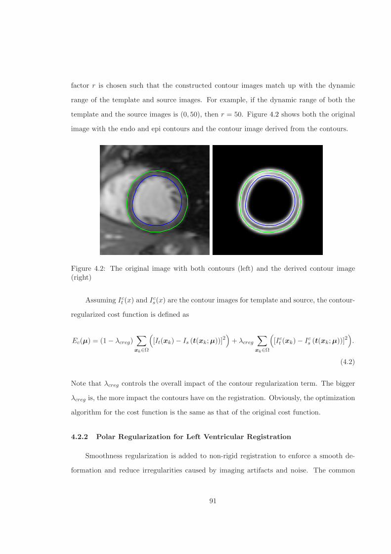
factor r is chosen such that the constructed contour images match up with the dynamic

range of the template and source images. For example, if the dynamic range of both the

template and the source images is (0, 50), then r = 50. Figure 4.2 shows both the original

image with the endo and epi contours and the contour image derived from the contours.

Figure 4.2: The original image with both contours (left) and the derived contour image(right)

Assuming Ict (x) and Ic

s(x) are the contour images for template and source, the contour-

regularized cost function is defined as

Ec(µ) = (1 − λcreg)∑

xk∈Ω

(

[It(xk) − Is (t(xk; µ))]2)

+ λcreg

∑

xk∈Ω

(

[Ict (xk) − Ic

s (t(xk; µ))]2)

.

(4.2)

Note that λcreg controls the overall impact of the contour regularization term. The bigger

λcreg is, the more impact the contours have on the registration. Obviously, the optimization

algorithm for the cost function is the same as that of the original cost function.

4.2.2 Polar Regularization for Left Ventricular Registration

Smoothness regularization is added to non-rigid registration to enforce a smooth de-

formation and reduce irregularities caused by imaging artifacts and noise. The common

91

practice is to define the smoothness in a Cartesian coordinate system. However, because

the Cartesian coordinate directions do not correspond to the primary directions of cardiac

deformation everywhere in the LV, the deformation field must be smoothed equally in both

x and y directions. The LV, however, usually thickens more in the radial direction than it

contracts in the circumferential direction. In this section, we propose a polar-coordinate

regularization term. With polar-coordinate regularization, different amounts of smoothing

can be applied in the radial and circumferential directions, which are the primary directions

of cardiac deformation.

First, the center of the LV is computed by averaging the LV endo and epi contours

points. Once the center point is defined, any point in the image can be defined in polar

coordinates with a radius and an angle. Let (x0, y0) be the center point. Let r and θ be

the radius and angle of an arbitrary point (x, y), then

r =√

(x− x0)2 + (y − y0)2, (4.3)

θ = arctany − y0

x− x0. (4.4)

With a circular assumption of the LV, the circumferential direction can be represented by

the angle of the tangential vector (the circumferential direction): θ +π

2.

At any point (x, y) in the optimization, the estimated deformation m(x, y) can be pro-

jected to the polar directions. The radial and circumferential components of the deformation

are

mr(x, y) = 〈(mx(x, y),my(x, y)), (cos θ, sin θ)〉 , (4.5)

mc(x, y) = 〈(mx(x, y),my(x, y)), (sin θ,− cos θ)〉 . (4.6)

This decomposition of the deformation is shown in Fig. 4.3.

Once the deformation is decomposed into the radial and circumferential directions,

we can measure their smoothness with their Laplacian. Hence the polar regularization is

92

θ

mr

mm

c

Figure 4.3: Polar decomposition of deformation

defined as

Erad =

∫ ∣∣∣∣

1

r2∂2mc

∂θ2+

1

r

∂

∂r

(

r∂mc

∂r

)∣∣∣∣

2

dxdy =

∫ ∣∣∣∣

1

r2∂2mc

∂θ2+

1

r

∂mc

∂r+∂2mc

∂r2

∣∣∣∣

2

dxdy (4.7)

and

Ecirc =

∫ ∣∣∣∣

1

r2∂2mr

∂θ2+

1

r

∂

∂r

(

r∂mr

∂r

)∣∣∣∣

2

dxdy =

∫ ∣∣∣∣

1

r2∂2mr

∂θ2+

1

r

∂mr

∂r+∂2mr

∂r2

∣∣∣∣

2

dxdy.

(4.8)

And the total polar regularization is

Epolar = λradErad + λcircEcirc, (4.9)

where λrad and λcirc are the weighting parameters for radial and circumferential smoothness.

From Eqs. (4.7) and (4.8), we see that the penalties Erad and Ecirc are defined continu-

ously. Hence we need to approximate them numerically. We use the most common method

93

of approximating a continuous integral with a finite sum, turning Eqs. (4.7) and (4.8) into

Erad =∑

(x,y)

∣∣∣∣

1

r2∂2mc

∂θ2+

1

r

∂

∂r

(

r∂mc

∂r

)∣∣∣∣

2

=∑

(x,y)

∣∣∣∣

1

r2∂2mc

∂θ2+

1

r

∂mc

∂r+∂2mc

∂r2

∣∣∣∣

2

(4.10)

and

Ecirc =∑

(x,y)

∣∣∣∣

1

r2∂2mr

∂θ2+

1

r

∂

∂r

(

r∂mr

∂r

)∣∣∣∣

2

=∑

(x,y)

∣∣∣∣

1

r2∂2mr

∂θ2+

1

r

∂mr

∂r+∂2mr

∂r2

∣∣∣∣

2

. (4.11)

The mathematical derivations of the gradient and Hessian of both Erad and Ecirc are

detailed in Section 4.2.2.

Gradient

Examining both Eqs. (4.10) and (4.11), we see that we need to derive∂mc

∂r,∂mr

∂r,

∂2mc

∂θ2,∂2mc

∂r2,∂2mr

∂θ2and

∂2mr

∂r2. Since both mc and mr can be represented with mx and my

as shown in Eqs. (4.5) and (4.6), we need to derive the derivatives of mx and my w.r.t. r

and θ as follows. The first order derivatives are

∂mx(x, y)

∂θ=∂mx

∂x

∂x

∂θ+∂mx

∂y

∂y

∂θ

=

[∂mx

∂x,∂mx

∂y

]

−r sin θ

r cos θ

,

∂mx(x, y)

∂r=

[∂mx

∂x,∂mx

∂y

]

cos θ

sin θ

,

∂my(x, y)

∂θ=

[∂my

∂x,∂my

∂y

]

−r sin θ

r cos θ

,

94

and

∂my(x, y)

∂r=

[∂my

∂x,∂my

∂y

]

cos θ

sin θ

.

The second order derivatives are

∂2mx

∂θ2=

∂

∂θ

(∂mx

∂x

∂x

∂θ+∂mx

∂y

∂y

∂θ

)

=

(∂2mx

∂x2

∂x

∂θ+∂2mx

∂x∂y

∂y

∂θ

)∂x

∂θ+∂mx

∂x

∂2x

∂θ2+

(∂2mx

∂y∂x

∂x

∂θ+∂2mx

∂y2

∂y

∂θ

)∂y

∂θ+∂mx

∂y

∂2y

∂θ2

=

⟨[∂2mx

∂x2,∂2mx

∂x∂y,∂2mx

∂y2,∂mx

∂x,∂mx

∂y

]

,

[(∂x

∂θ

)2

, 2∂x

∂θ

∂y

∂θ,

(∂y

∂θ

)2

,∂2x

∂θ2,∂2y

∂θ2

]⟩

,

∂2my

∂θ2=

⟨[∂2my

∂x2,∂2my

∂x∂y,∂2my

∂y2,∂my

∂x,∂my

∂y

]

,

[(∂x

∂θ

)2

, 2∂x

∂θ

∂y

∂θ,

(∂y

∂θ

)2

,∂2x

∂θ2,∂2y

∂θ2

]

, ,

⟩

∂2mx

∂r2=

⟨[∂2mx

∂x2,∂2mx

∂x∂y,∂2mx

∂y2,∂mx

∂x,∂mx

∂y

]

,

[(∂x

∂r

)2

, 2∂x

∂r

∂y

∂r,

(∂y

∂r

)2

,∂2x

∂r2,∂2y

∂r2

]⟩

,

and

∂2my

∂r2=

⟨[∂2my

∂x2,∂2my

∂x∂y,∂2my

∂y2,∂my

∂x,∂my

∂y

]

,

[(∂x

∂r

)2

, 2∂x

∂r

∂y

∂r,

(∂y

∂r

)2

,∂2x

∂r2,∂2y

∂r2

]

, .

⟩

95

Using a commercially available symbolic computation software, we get

∂2mc

∂θ2=

⟨[∂2mx

∂x2,∂2mx

∂x∂y,∂2mx

∂y2,∂mx

∂x,∂mx

∂y,mx

]

,

[

−r2 sin3 θ, 2r2 sin2 θ cos θ,−r2 sin θ cos2 θ, 3r sin θ cos θ, r sin2 θ − 2r cos2 θ, sin θ

]⟩

+

⟨[∂2my

∂x2,∂2my

∂x∂y,∂2my

∂y2,∂my

∂x,∂my

∂y,my

]

,

[

r2 sin2 θ cos θ,−2r2 sin θ cos2 θ, r2 cos3 θ,−r cos2 θ + 2r sin2 θ,−3r sin θ cos θ,− cos θ

]⟩

.

Plugging in the derivatives of B-spline representations of mx and my w.r.t. the control

points µxi and µyi, we get

∂2mc

∂θ2=∑

i

µxi

(

(−r2 sin3 θ)ψiβi + (2r2 sin2 θ cos θ)ξiξi + (−r2 sin θ cos2 θ)βiψi+

(3r sin θ cos θ)ξiβi + (r sin2 θ − 2r cos2 θ)βiξi + sin θβiβi

)

+

∑

i

µyi

(

(r2 sin2 θ cos θ)ψiβi + (−2r2 sin θ cos2 θ)ξiξi + (r2 cos3 θ)βiψi+

(−r cos2 θ + 2r sin2 θ)ξiβi + (−3r sin θ cos θ)βiξi + (− cos θ)βiβi

)

, (4.12)

where the abbreviations such as ψiβi are defined in an orderly fashion where the first is

w.r.t. x and the second is w.r.t. y. For example,

ψiβi = ψ(x− xi)β(y − yi). (4.13)

Also the functions ξ and ψ are first and second derivatives of the B-spline basis β,

ξ(x) =dβ(x)

dx, (4.14)

and

ψ(x) =d2β(x)

dx2. (4.15)

96

In a similar fashion, we get

∂2mc

∂r2=∑

i

µxi

(

(− sin θ cos2 θ)ψiβi + (−2 sin2 θ cos θ)ξiξi + (− sin3 θ)βiψi

)

+

∑

i

µyi

(

(cos3 θ)ψiβi + (2 sin θ cos2 θ)ξiξi + (sin2 θ cos θ)βiψi

)

, (4.16)

and

∂2mr

∂θ2=∑

i

µxi

(

(r2 sin2 θ cos θ)ψiβi + (−2r2 sin θ cos2 θ)ξiξi + (r2 cos3 θ)βiψi+

(2r sin2 θ − r cos2 θ)ξiβi + (−3r sin θ cos θ)βiξi + (− cos θ)βiβi

)

+

∑

i

µyi

(

(r2 sin3 θ)ψiβi + (−2r2 sin2 θ cos θ)ξiξi + (r2 sin θ cos2 θ)βiψi+

(−3r sin θ cos θ)ξiβi + (−r sin2 θ + 2r cos2 θ)βiξi + (− sin θ)βiβi

)

, (4.17)

and

∂2mr

∂r2=∑

i

µxi

(

(cos3 θ)ψiβi + (2 sin θ cos2 θ)ξiξi + (sin2 θ cos θ)βiψi

)

+

∑

i

µyi

(

(sin θ cos2 θ)ψiβi + (2 sin2 θ cos θ)ξiξi + (sin3 θ)βiψi

)

. (4.18)

Notice that in the above, ψ is the 2nd derivative of the B-spline β.

If we plug Eqs. (4.12), (4.16), (4.17) and (4.18) into Eq. (4.10) and combine similar

terms w.r.t. the B-spline control points, we get an equation in the following form,

Erad =∑

(x,y)

∣∣∣∣∣∣

∑

i

sxi(x, y)µxi +∑

j

syj(x, y)µyj

∣∣∣∣∣∣

2

, (4.19)

where sxi and syj are the combined weights for µxi and µyj . Using the linear index k

instead of the sample points (x, y), putting the B-spline control points into a single vector

form µ = [µx1, µx2, . . . , µxn, µy1, µy2, . . . , µyn]T and the weights into vector form s(k) =

97

[sx1(x, y), sx2(x, y), . . . , sxn(x, y), sy1(x, y), sy2(x, y), . . . , syn(x, y)]T , we get

Erad =∑

k

(sT

k µ)2

(4.20)

=

∥∥∥∥∥

[

s1, s2, . . . , sn

]T

µ

∥∥∥∥∥

2

2

(4.21)

= µTSST µ, (4.22)

where S =

[

s1, s2, . . . , sn

]

is the weighting matrix. Differentiating (4.22) once, we get the

gradient of Erad

∇Erad = 2SST µ. (4.23)

Differentiating Eq. (4.23) once, we get the Hessian of Erad

∆Erad = 2SST . (4.24)

We can see from Eqs. (4.24) and (4.23) that the Hessian of Erad is a constant matrix and

the gradient is just the Hessian matrix multiplying the B-spline control point vector. This

observation is important since it tells us that we can improve computation efficiency by

precomputing the Hessian matrix and reusing it in the iterations.

Both the gradient and Hessian of the circumferential cost Ecirc can also be derived

similarly. If we let

∇Ecirc = 2UUT µ (4.25)

and

∆Ecirc = 2UUT , (4.26)

98

then we can write the gradient and Hessian of the polar regularization defined in Eq. (4.9)

as

∇Epolar = 2(λradSST + λcircUU

T )µ (4.27)

and

∆Epolar = 2(λradSST + λcircUU

T ). (4.28)

4.2.3 Custom Shape Regularization for Right Ventricular Registration

The circular assumption for the LV is no longer valid for the complicated shape of

the RV. However, we can still utilize the basic concept of the polar regularization for LV

and generalize it to RV registration. Even though the RV assumes a more complicated

shape than the LV, the deformation of the RV free wall in the short-axis images can still be

decomposed into two principle directions, the normal direction and the tangential direction

w.r.t. the RV wall curve. The normal direction corresponds to the radial direction in the case

of LV registration, and the tangential direction corresponds to the circumferential direction.

We generalize the polar regularization for the LV by fitting a circle at every point along

the RV free wall and regularize the RV deformation along the radial and circumferential

directions of the fitted circle. As the point on the RV free wall progresses, the fitted circle

changes in both location and radius. An illustration of the generalization is shown in Fig.

4.4.

At any point along the RV free wall, the radius of the fitted circle r is directly related

to the curvature κ of the RV free wall at that point. Specifically,

κ =1

r. (4.29)

99

Figure 4.4: Custom shape regularization for RV registration: fitting circles at differentpoints

That is, the bigger the radius of the fitted circle, the smaller the curvature of the RV free

wall at that point and vice versa.

The above defines curvature along the RV free wall. For image registration, we need

to have the curvature at any pixel locations in the image. This is achieved by scaling the

curvature at the RV free wall based on the distance of the pixel location to the center of the

RV contours. Note here the center of the RV contours is not defined the same way as the

LV center. Since the RV contour is is concave at the septum, the usual way of computing

the center by averaging the contour points will likely give a center point that is outside the

RV contour or very close to the septum. Using a center like this to scale the RV contour

shape may result in distorted shapes. We choose the RV center point by finding the middle

point of a line segment that connects the approximate center point of the septum with the

approximate center point of the free wall. Then at any pixel location, the curvature at

the pixel is defined by scaling the normalized curvature computed from the normalized RV

100

contour. This is illustrated in Fig. 4.5, where the contour is scaled w.r.t. the RV center

and plotted. The curvature at a pixel is the curvature at the point of the corresponding

contour.

Figure 4.5: Curvature illustration of custom shape regularization.

The normal and circumferential directions at any point in the image is determined

similarly with the scaling. Figure 4.6 shows the normal directions at selected pixel locations

covering the RV region.

The mathematical description of the custom shape regularization is similar to that of

the polar regularization. For the custom shape regularization, the regularization weighting

parameters for normal and tangential directions are named λnn and λtt. They play the same

roles as λrad and λcirc in the polar regularization case. The reader is referred to Section

4.2.2 for the detailed derivations.

4.3 Strain Computation from Myocardial Deformation

After the registrations, we get a series of estimated motions uk(x), k = 0, 1, . . . , n where

n+ 1 is the number of frames in the cardiac cycle. uk(x) maps the sampling points in the

(k − 1)-th image frame at time tk−1 to the k-th image frame at time tk except for k = 0,

101

Figure 4.6: Normal directions of custom shape regularization overlaid with short-axis imageof the RV region.

where u0(x) maps the sampling points in the last image frame at tn to the first image frame

at t0. With these deformations, one can trace any points throughout the cardiac cycle. Let

vk(x) be the accumulated motion at time tk.

For easy of description, let us compute the deformation at time tk, k ∈ 1, 2, . . . , n.

Assuming the first frame at t0 is at end-diastole (ED) and define any material point at ED

as x0 = X, the spatial point of X at t1 and t2 are x1 and x2 respectively. First frame

motion is u1(x0), and second frame motion is u2(x1). Then we have,

x1 = X + u1(X) = X + v1(X) (4.30)

and

dv1(X)

dX=du1(X)

dX. (4.31)

102

Similarly, we can write

x2 = X + v2(X)

= x1 + u2(x1)

= X + [u1(X) + u2(x1)]

= X + [u1(X) + u2(X + u1(X))]

and

du2(X)

dX=du1(X)

dX+du2(x1)

dx1

dx1

dX

∣∣∣∣x1=X+u1(X)

=du1(X)

dX+du2(x1)

dx1(I +

du1(X)

dX)

=

(du2(x1)

dx1+ I

)(du1(X)

dX+ I

)

− I

Similarly, at time t3, we can get,

dv3(X)

dX=

(du3(x2)

dx2+ I

)(du2(x1)

dx1+ I

)(du1(X)

dX+ I

)

− I

In general, for k ≥ 1, we get the displacement gradient at X at time tk as

dvk(X)

dX=

(duk(xk−1)

dxk−1+ I

)(duk−1(xk−2)

dxk−2+ I

)

· · ·

(du1(X)

dX+ I

)

− I

The Lagrangian strain tensor is defined as

E =1

2(F T

k Fk − I), (4.32)

103

where Fk =dvk(X)

dX+I is the deformation gradient. In 2D, Fk and I are both 2×2 matrices,

dv1(X)

dX=

dv1,x

dx

dv1,x

dydv1,y

dx

du1,y

dy

. (4.33)

Since the material point X is tracked throughout the cardiac cycle, any tracking error

will accumulate as the propagation goes away from ED. Hence the error as a function of

time would be increasing from ED to the final frame. To alleviate the error accumulation,

we can track the material points in both directions and then combine both the forward and

backward deformations. This way the error as a function of time would be decreased in the

cardiac cycle. Note that no inverse of deformation is needed in this process. We have chosen

to average the forward and backward deformation gradients (Fk,f and Fk,b respectively) at

time tk, k = 1, 2, . . . , n, as

Fk = ωFk,f + (1 − ω)Fk,b,

where ω is the weight determined by the tk. Then the strain is computed as

Ek =1

2

(F T

k Fk − I)

(4.34)

=1

2

(1

4(F T

k,fFk,f + F Tk,bFk,b + F T

k,fFk,b + F Tk,bFk,f ) − I

)

. (4.35)

From (4.35), we see that the Lagrangian strain tensor is also a 2 × 2 matrix in 2D.

The directional strains can then be computed by rotating the 2D tensor. For example,

let θ be the angle of the radial direction, then the rotated strain tensor is

Erotate = RERT , (4.36)

104

where R is the rotation matrix

R =

cos θ sin θ

− sin θ cos θ

. (4.37)

The radial strain Err and the circumferential strain Ecc are

Err = Erotate(1, 1) (4.38)

Ecc = Erotate(2, 2). (4.39)

One can also compute the minimum strain Emin and the maximum strain Emax, which

are defined as the minimum and maximum eigenvalues of the strain tensor E .

4.4 Left and Right Ventricular Strain Results

The proposed algorithms for measuring ventricular strains are examined on MR images

from both normal volunteers and patients. First, we test the performance of the contour

regularization and polar regularization for left ventricular strain in Sections 4.4.1, 4.4.2 and

4.4.3. Then the custom shape regularization algorithm is tested for right ventricular strain

in Sections 4.4.4 and 4.4.5.

4.4.1 Contour Regularization for LV Strains

38 normal human volunteers and 42 patients with myocardial infarction (MI) were

scanned with both standard cine and tagged MRI. Circumferential and radial strains and

strain rates were computed from the cine data with the algorithm described above, which

was implemented in MATLAB. Approximately 7 minutes per study was needed to propagate

contours, and another 7 minutes was needed to refine the interframe deformations on a 2.6

GHz dual-core personal computer with 4 Gb of RAM. The same strains were computed

from the tagged data using 2-D HARP analysis [63] and 3-D model-based analysis [44].

105

0 0.2 0.4 0.6 0.8 10

0.2

0.4

0.6

0.8

1

λ

Ecc

co

rre

lati

on

co

e!

cie

nt

Figure 4.7: Correlation coefficient between mid-ventricular circumferential strain (Ecc) com-puted from cine MRI and tagged MRI using HARP analysis for different values of thecontour regularization parameter (λcreg). Correlation computed over training data.

To evaluate the effect of λcreg, 20 normal and 20 MI patients were randomly selected.

Strains were computed from the cine data with different values of λcreg without polar

regularization. The results are shown in Fig. 4.7. λcreg = 0 corresponds to the case where

contour-based regularization was not used to refine the interframe deformation. Increasing

values of λcreg reflect an increasing influence of the contour term in (4.2) on the result.

Based on the above observation, we chose λcreg = 0.1 and evaluated our algorithm

on another set of 38 studies (18 normals and 20 MI patients) by comparing to both 3-D

model-based analysis [44] and HARP. The correlation coefficient between mid-ventricular

end-systolic circumferential strain (Ecc) computed from cine MRI and tagged MRI with

3-D model-based analysis was good (ρ=0.83). The correlation coefficients between cine

MRI and HARP Ecc, systolic Ecc rate, and early diastolic Ecc rate were 0.84, 0.73, and

0.61, respectively. The reduced correlation in systolic Ecc rate is most likely because tagged

MRI introduces contrast inside the myocardium whereas, in cine MRI, deformation must

be estimated primarily from the deformation of the myocardial boundaries. This is also

106

true in early diastole, but the contrast in tagged MRI has faded considerably by this point.

In cine MRI, however, myocardial boundary contrast is relatively constant throughout the

cardiac cycle. The early diastolic Ecc rate computed from cine MRI may indeed be superior

to that computed from tagged MRI, but more analysis is needed to support this claim.

Fig. 4.8a shows both cine and HARP mid-ventricular Ecc versus normalized time

averaged over the 18 normal human volunteers. Time was normalized so that zero corre-

sponds to end-diastole and 100 corresponds to peak early diastolic circumferential strain.

The curves are fairly close together, with the exception of the inferior wall where cine MRI

tends to over-estimate strain. Fig. 4.8b shows the same type of curve for radial strain (Err).

The cine-based algorithms consistently estimates higher radial strains than HARP. Tagged

MRI, however, is known to produce poor estimates of radial strain. The peak cine-MRI

Err, however, is closer to wall thickness measurements in these subjects (61±2.6%). This

result suggests that the cine-MRI strain may be a more accurate estimate of radial strain

than those computed from tagged MRI.

4.4.2 Preliminary Study of LV Strains with Hypertensive Patients

In cine data, strains can be measured during diastole. In tagged MRI, the tag pattern

fades with time and measurements of strain during diastole are often unreliable — partic-

ularly in late diastole when the left atrium contracts. Consequently, to validate the cine

strains in diastole, strains were computed from standard cine MRI scans of 39 normal hu-

man volunteers and compared to 45 patients with hypertension. Patients with hypertension

often have diastolic dysfunction. Diastolic dysfunction occurs when the heart wall becomes

stiff, and the LV filling rate is reduced. In normals, filling mostly occurs during passive

relaxation of the ventricle in early diastole. In patients with diastolic dysfunction, however,

early diastolic filling is reduced and more filling occurs during the atrial contraction phase.

Figure 4.9. shows the early and atrial diastolic circumferential expansion rates in both

normals and hypertensive patients. In early diastole, circumferential expansion in hyper-

tensives is lower than normal. In atrial diastole, circumferential expansion is higher than

107

Ant

-0.2

0.2

AntSep InfSep Inf InfLat AntLat

(a)Ant

0

0.4


(b)

Figure 4.8: Mid-ventricular circumferential (a) and radial (b) strains versus time computedfrom cine MRI (red) and tagged MRI/HARP (blue). Time normalized to the range 0 (end-diastole) to 100 (early diastole). The curves represent an average (solid) and ± standarderror (dotted) over 18 normal human volunteers.

normal. This observation of early to atrial reversal in hypertensive patients is consistent

with clinical measurements of mitral-valve inflow rates with Doppler ultrasound [77].

4.4.3 Polar Regularization for LV Strains

38 normal human volunteers and 42 patients with myocardial infarction (MI) were

imaged with an SSFP sequence with the following parameters: TR 3.8, TE 1.6 ms, slice

thickness 8mm, no inter-slice spacing, flip angle 45 deg, k-space segmentation 10 views per

segment, matrix 256 × 128, field of view 42 cm, 1 signal average, bandwidth 125kHz. LV

contours were drawn at ED and ES for all valid short-axis slices semi-automatically by

trained experts. Radial and circumferential strains were then computed in all studies using

both contour regularization and polar regularization. A training set of 18 normal and 22

MI patients was used to choose λrad and λcirc (Eq. (4.9)). An evaluation set of 20 normals

and 20 MIs were used to compare the circumferential strains with strains computed using

108

Nrm HTN

0

10

20

30

40

50

60

70

80

90

E Dia Cine Circ Strain Rate

%/s

ec

*

Nrm HTN

0

5

10

15

20

25

30

35

40

45

A Dia Cine Circ Strain Rate

%/s

ec

*

(a) (b)

Figure 4.9: Circumferential expansion rates in early (a) and atrial (b) diastole in normalhuman volunteers (Nrm) and patients with hypertension (HTN). ∗P < 0.05 vs. normal.

HARP analysis and the 3D model-based method. Radial strains were not compared with

HARP or 3D model-based analysis because radial strains computed from tagged MRI were

unreliable.

Figure 4.10 shows plots of circumferential strain versus time computed using both

contour and polar regularization and HARP averaged over the 20 normal human volunteers

in the evaluation set. Time was normalized in these plots so that zero corresponds to end-

diastole and 100 corresponds to early diastole. The cine strain agrees with HARP at all

levels, but the agreement is particularly good at mid-ventricle. Strains past early diastole

are not shown because HARP strains were not reliable past early diastole due to tag fading.

Comparing Fig. 4.10 to Fig. 4.8a, one can see that the strain discrepancy in the inferior

septum segment is reduced and the strains are overall smoother than the results with only

contour regularization.

109

Ant

Ba

se

−0.2

0.2


Mid

−0.2

0.2

Ap

ex

−0.2

0.2

Figure 4.10: Circumferential strains vs. time computed from cine MRI (red) and taggedMRI/HARP (blue). The curves represent the average (solid) and ± standard error (dotted)over 20 normal human.

Figure 4.11 shows the deformations estimated between two frames of the short-axis

images with contour regularization only and with both contour regularization and polar

regularization. For easy viewing, only the deformation inside the LV epi contour are shown

in the figure. Comparing the two deformations, one can see that the polar regularization

helps to smooth the estimated deformations in the polar directions and reduces registration

artifacts.

Figure 4.12 shows circumferential cine strain overlaid on a mid-ventricular short-axis

slice for all imaged time frames in a normal human volunteer. As expected, contraction

increases through systole and decrease during diastole. Strain is greater in the lateral wall

than the septal wall, and strain is greater near the endocardium than near the epicardium

110

(a) (b)

Figure 4.11: Estimated deformation without (a) and with (b) polar regularization betweentwo frames of short-axis images.

4.4.4 RV Strain Measurement

Due to the complicated shape and the thin wall of the right ventricle, we have chosen to

use the consistent image registration with the inverse consistency regularization (described

in Section 2.4.1 and Section 2.4.2); the topology preservation regularization (described in

Section 2.4.1 and Section 2.4.3) and the custom shape regularization (described in Section

4.2.3). The general effects of both the inverse consistency regularization and the topology

preservation regularization have been studied in Section 2.6 of Chapter 2. In this section,

we will demonstrate the effects of all three regularizations on the RV registration. We do

this by test registering two short-axis images from a mid-ventricular slice. Note that we

deliberately took the ED image and the ES image so that the deformation between them

is significant. This helps expose any potential problems in the registration algorithm more

than if we took two adjacent images with little difference.

111

Figure 4.12: Circumferential strain overlaid on a mid-ventricular slice of a normal humanvolunteer. Yellow represents no contraction, red represents 10% contraction and blue rep-resents 20% contraction. Time increases from left to right starting from the upper-leftcorner.

Effects of Topology Preservation Regularization

The two images are registered with λic = 0 and λcsr = 0. In other words, there is no

inverse consistency regularization or custom shape regularization.

First, the topology preservation regularization parameter λtopo can have a wide range

of values. However, of great importance is the design of the penalizing function defined in

Eq. (2.28). We have chosen a = 0.01 and c = 10 to ensure a steeper slope at the lower

end of the acceptable range of the Jacobian determinant values. As we have pointed out in

Section 2.4.1, this helps to prevent topology change during registration.

112

For cardiac registration, the myocardium contraction or expansion is quite limited

(usually below 30% in the tangential directions and below 50% in the normal directions).

Figure 4.13 compares the registration results with bu = 2, bl = 0.5 and bu = 5, bl = 0.2

with everything else fixed (λtopo = 10−3). Recall that bu and bl are the upper and lower

bounds of the flat range of the topology preservation penalizing function 2.28. One can

easily see that bu = 2, bl = 0.5 gives a much better registration results for the RV. Hence

we have chose to have the upper bound bu = 2 and bl = 0.5, which corresponds to 200%

expansion and 50% contraction.

With the above chosen topology preservation penalizing function, we tested the effects

of changing λtopo. Figure 4.14 shows the registration results with λtopo = 10−5 and λtopo =

10−3. We see that λtopo = 10−5 is too weak a regularization that it does not improve the

registration in terms of topology preservation.

In both the above registrations, notice that the topology preservation regularization

with proper weights helps with the inverse consistency of the estimated deformations. This

shows that topology preservation is a valid assumption that contributes to improving the

registration accuracy.

Effects of Custom Shape Regularization

In a similar fashion to the testing of topology preservation in Section 4.4.4, we study

the effect of custom shape regularization on the RV registration. In this case, both the

inverse consistency regularization and the topology preservation regularization are turned

off. λtt = 10−4 and λnn = 10−5 were used in this experiment. Like the case in the polar

regularization for LV strain computation, we have chosen a bigger regularization weight for

the tangential direction than the normal direction since tangential deformation artifacts

usually lead to twisting of the myocardium, which is not desirable and best avoided. The

results are shown in Fig. 4.15. Observe that the custom shape regularization fulfills its

role by generating a more satisfactory result than the no-regularization case. Again, we see

113

(a) (b)

Figure 4.13: Registration results with bu = 2, bl = 0.5 (a) and bu = 5, bl = 0.2 (b).First row: template image and source image; Second row: deformed source image andtemplate image; Third row: absolute residue error between the first two rows; Last row:deformed regular grid by the combined deformations (forward-backward and backward-forward) plotted on original images.

that the custom shape regularization helps with the inverse consistency of the estimated

deformations. Also, it helps to preserve the topology of the image structure.

114

(a) (b)

Figure 4.14: Registration results with λtopo = 10−5 and λtopo = 10−3, both ordered thesame way as that in Fig. 4.13.

4.4.5 RV Strain Results for Patient Population

As we have stated earlier, we chose the custom shape regularization weighting pa-

rameter λtt to be 10 times bigger than λtt to enforce more on circumferential deformation

smoothness. Hence we have λtt = 10λnn. In the following, we will assume this relationship

and refer only λtt.

115

(a) (b)

Figure 4.15: Registration results without (a) and with (b) custom shape regularization,both ordered the same way as that in Fig. 4.13.

Based on test RV registrations on cardiac cine MR images, we found that λtopo can

assume a wide range of values as long as it is not too small (for example, λtopo = 10−5

was too small in the test registration in Section 4.4.4), all of which give good registration

performance. This is because it will only be triggered in the registration when the topology

constraint is violated. For the following analysis, we choose λtopo = 0.1. Also, for RV,

we have chosen the lower and upper bounds of the flat region of the topology preservation

116

penalizing function p(x) (see Eq. (2.28)) to be bl =1

3and bu = 3, which should be flexible

enough to track RV wall deformation.

We have found the reasonable ranges for the weighting parameters λic and λtt by exam-

ining test registrations of the RV. Specifically, the reasonable range for λic is (10−4, 10−2),

and the reasonable range for λtt is (10−6, 10−4). So we chose combinations of elements from

the following parameter sets for testing:

Λic = 0, 10−4, 5 × 10−4, 10−3, 10−2 (4.40)

and

Λtt = 0, 10−6, 5 × 10−6, 10−5, 10−4. (4.41)

In other words, the parameter combination (λic, λtt) ∈ Λic × Λtt.

Fourteen studies consists of 6 normal volunteers, 2 mitral regurgitation patients and 6

pulmonary hypertensive patients were used to test the registration algorithm with the above

parameter sets. We computed correlation coefficients between the maximum tangential mid-

ventricular strains (maximum tangential stretching) computed from cine MR images using

the proposed algorithm and tagged MR images using HARP. They are shown in Table 4.1.

We can see that all the tested parameter combinations generated good correlation between

the two being compared. However, statistically neither the inverse consistency or custom

shape regularizations improve the estimate of the RV tangential strains. This does not

invalidate the positive effects of the two regularizations on an individual basis. As we have

seen above, without the regularizations, the registration results are much poorer, which is

not being reflected in this peak strain correlation analysis.

Note that the HARP algorithm for RV strain computation is not an ideal candidate

for testing our algorithm. This is illustrated in Fig. 4.16, which shows the tangential strain

vs. time curves for different segments of the RV for a normal volunteer. One can see

117

Table 4.1: Correlation coefficients between peak circumferential strains computed from cineand tagged MR images using the proposed algorithm and HARP. First row shows the valuesof λtt and first column shows the values of λic.

0 5 × 10−6 10−5 5 × 10−5 10−4

0 0.77 0.77 0.77 0.77 0.7810−4 0.77 0.77 0.78 0.77 0.78

5 × 10−4 0.78 0.78 0.78 0.78 0.7910−3 0.78 0.78 0.78 0.78 0.7910−2 0.78 0.78 0.78 0.80 0.80

that the HARP measurement is very noisy, which renders it unreliable for individual strain

measurements. From this perspective, our algorithm gives a much better indication of the

RV strains, especially for the mid-ventricular slices, which experiences less through-plane

motion. For the basal and apical slices, due to significant through-plane motion, the 2D

strain measurement could be inaccurate. This is clearly seen for the apical slices. As the

ventricle contracts longitudinally, the apices of the ventricles move toward the base. In the

short-axis view, this generates the illusion that the ventricles are experiencing significant

contraction, which leads to higher estimated 2D strains.

Ant

−0.2

0.2

Lateral Inferior

−0.2

0.2

−0.2

0.2

Figure 4.16: RV circumferential strains vs. time plot of a normal volunteer: comparingproposed algorithm (red) and HARP (blue)

118

From the above experiments, we can see that the registration results are not very

sensitive to the weights of the regularization parameters. To preserve the benefits brought by

the regularizations for analysis of individual studies, we have decided that λic = 10−3, λtt =

5 × 10−5 was a good choice for RV registration.

Ant

−0.2

0.2Lateral Inferior

−0.2

0.2

−0.2

0.2

Figure 4.17: RV circumferential strains vs. time plot for 34 studies computed from cineMRI (red) and tagged MRI/HARP (blue). The strains from cine MR images were computedusing the proposed algorithm with λtopo = 10−1, λic = 10−3, and λtt = 5∗10−5. The curvesrepresent the average (solid) and ± standard error (dotted).

Figure 4.17 shows the RV circumferential strain vs. time plots for 34 studies with the

chosen regularization weights (λtopo = 10−1, λic = 10−3, λtt = 5×10−5). Of the 34 studies,

16 are normal volunteers, 4 are mitral regurgitation patients and the rest 14 are pulmonary

hypertension patients. We see that the circumferential strain curves computed from cine

MRI using the proposed algorithm is lower than that from tagged MRI using HARP. How-

ever, as we have seen in Fig. 4.16, the HARP measurements for RV are unreliable. So one

can not say which one is better.

119

Chapter 5

Conclusion

In this dissertation, a group of methods for various cardiac functional analysis with cine

magnetic resonance imaging (MRI) based on non-rigid image registration was described.

The importance of cardiac functional analysis is evident as cardiac disease has been the

leading cause of death in the United States for many years. Cardiac MR imaging is a non-

invasive, radiation-free technology that is able to acquire good-quality images of the beating

heart with a good time resolution. Functional analysis with cardiac MR imaging can be

divided into three major categories: global ventricular volumetric measurements such as

left and right ventricular end-diastolic and end-systolic volumes; local ventricular curvature

measurements and local myocardium strain measurements.

The global volumetric measurements are usually derived from cine MR images, which

provides good-quality soft-tissue contrast throughout the cardiac cycle. The volumetric

analysis methods are based on myocardium segmentation. While many automatic my-

ocardium segmentation algorithms have been proposed, most of them are unreliable and

need constant user corrections. Semi-automatic segmentation algorithms requires some user

interaction but can be much more robust in performance. We have proposed a dual-contour

propagation algorithm that takes advantage of both the end-diastole and end-systole con-

tours usually drawn at most institutions. The dual-contour propagation algorithm combines

the user input at both end-diastole and end-systole and can successfully identify the papil-

lary muscles, which is the major cause of segmentation failures for automatic segmentation

methods. Our results show that the volumetric measurement from the dual-contour prop-

agation algorithm is statistically equivalent to that derived from manual segmentation.

120

The local curvature measurements of the ventricular wall can also be derived from the

myocardium segmentation. From this perspective, it can be included in the same category

as the above global volumetric measurements.

The local myocardium strain analysis provide information about the dynamic contrac-

tion and relaxation of the different myocardium segments and is very valuable information

for clinical diagnosis and treatment of cardiac disease. Conventionally, the cardiac strains

measurements are derived from tagged MR images, which provides contrast inside the my-

ocardium during the early half of the cardiac cycle. However, the tagged MR images are

not easy to acquire and can be very noisy. Furthermore, the tag lines can not be spaced

too close due to physical limitations. This means only a few tag lines can be placed inside

the myocardium and and tracked. The deformation of the other areas of the myocardium

has to be interpolated for strain analysis. Lastly, as mentioned above, the tag lines fade

quickly, and usually it is of reasonable quality only for about half of the cardiac cycle. This

makes it useless for assessing diastolic functional parameters of the heart. Cine MR images,

on the other hand, have good quality throughout the cardiac cycle. We propose several

novel regularization algorithms to reduce artifacts from the registration. This includes the

contour regularization and the polar regularization algorithms for left-ventricular strain

analysis and custom shape regularization for right-ventricular strain analysis.

All of the above analysis is based on non-rigid image registration. Traditional non-rigid

registration algorithms are biased, since they only estimate single-directional deformations.

Consistent image registration solves this problem by coupling estimation of deformations

in both directions. However, many of the existing consistent image registration algorithms

requires inversion of deformations during optimization, which takes a lot of computation

time. In this dissertation, we propose a consistent image registration algorithm with B-spline

deformation model that does not need inversion of deformations. The problem is solved by

a second-order optimization algorithm using both the gradient and Hessian of the cost

function. A new topology-preserving regularization is proposed that can accommodate a

wide variety of applications. Finally, we propose an efficient adaptive optimization algorithm

121

to improve computation efficiency while retaining the registration accuracy. We proposed a

divide-and-conquer strategy for deformations with large degree of freedom. The proposed

adaptive and topology-preserving consistent image registration algorithm was tested on

both cardiac and brain images.

In summary, we have proposed a host of algorithms based on non-rigid image regis-

tration for cardiac functional analysis with cine MR imaging. Promising results have been

presented. Our future work includes extending the current algorithms to 3 dimensions and

intra-model registration and analysis.

122

Bibliography

[1] V. Arsigny, O. Commowick, X. Pennec, and N. Ayache. A log-euclidean framework forstatistics on diffeomorphisms. In Proc. of MICCAI’06 - LNCS 4190, pages 924–931,2006.

[2] J. Ashburner, J. Andersson, and K. Friston. Image registration using a symmetricprior - in three dimensions. Human Brain Mapping, 9(4):212–225, 2000.

[3] B. B. Avants, C. L. Epstein, M. Grossman, and J. C. Gee. Symmetric diffeomorphicimage registration with cross-correlation: Evaluating automated labeling of elderlyand neurodegenerative brain. Medical Image Analysis, 2007.

[4] L. Axel and L. Dougherty. Heart wall motion: improved method of spatial modulationof magnetization for MR imaging. Radiology, 172(2):349–360, 1989.

[5] M. F. Beg and A. Khan. Symmetric data attachment terms for large deformationimage registration. IEEE Trans Med Imaging, 26(9):1179–89, 2007.

[6] N. G. Bellenger, L. C. Davies, J. M. Francis, A. J. Coats, and D. J. Pennell. Reductionin sample size for studies of remodeling in heart failure by the use of cardiovascularmagnetic resonance. J Cardiovasc Magn Reson, 2(4):271–8, 2000.

[7] A. Bistoquet, J. Oshinski, and O. Skrinjar. Left ventricular deformation recovery fromcine MRI using an incompressible model. IEEE Transactions on Medical Imaging,26(9):1136–1153, Sep. 2007.

[8] T. Blu and M. Unser. Approximation error for quasi-interpolators and (multi-) waveletexpansions. Applied and Computational Harmonic Analysis, 6(2):219–251, March1999.

[9] R. O. Bonow, S. L. Bacharach, M. V. Green, K. M. Kent, D. R. Rosing, L. C. Lipson,M. B. Leon, and S. E. Epstein. Impaired left ventricular diastolic filling in patientswith coronary artery disease: assessment with radionuclide angiography. Circulation,64(2):315–23, 1981.

[10] F. Bursi, S. A. Weston, M. M. Redfield, S. J. Jacobsen, S. Pakhomov, V. T. Nkomo,R. A. Meverden, and V. L. Roger. Systolic and diastolic heart failure in the community.Journal of the American Medical Association, 296(18):2209–16, 2006.

[11] Pascal Cachier and David Rey. Symmetrization of the non-rigid registration problemusing inversion-invariant energies: Application to multiple sclerosis. In MICCAI,pages 472–481, 2000.

123

[12] C. Cassen, J. Domenger, J. Braquelaire, and J. Barat. Left ventricular segmentationin MRI images. In Proceedings of the 2nd International Symposium on Image and

Signal Processing and Analysis, pages 244–249, 2001.

[13] R. Chandrashekara, R. Mohiaddin, and D. Rueckert. Analysis of 3-D myocardialmotion in tagged MR images using nonrigid image registration. IEEE Transactions

on Medical Imaging, 23(10):1245–1250, 2004.

[14] W. Chen, S. Zhou, and B. Liang. LV contour tracking in MRI sequences based on thegeneralized fuzzy GVF. In International Conference on Image Processing, volume 1,pages 373–376 Vol. 1, 2004.

[15] G. Christensen. Consistent linear-elastic transformations for image matching. Lecture

Notes in Computer Science, 1613:224–237, 1999.

[16] G. Christensen and H. Johnson. Consistent image registration. IEEE Transaction on

Medical Imaging, 20(7):568–82, 2001.

[17] L. D. Cohen. On active contour models and balloons. Computer Vision, Graphics,

and Image Processing. Image Understanding, 53(2):211–218, 1991.

[18] A. Collignon, F. Maes, D. Delaere, D. Vandermeulen, P. Suetens, and G. Marchal. Au-tomated multi-modality image registration based on information theory. Information

Processing in Medical Imaging, pages 263–274, 1995.

[19] T. F. Cootes, G. J. Edwards, and C. J. Taylor. Active appearance models. Lecture

Notes in Computer Science, 1407:484, 1998.

[20] T. F. Cootes, C. J. Taylor, D. H. Cooper, and J. Graham. Active shape modelstheirtraining and application. Comput. Vis. Image Underst., 61(1):38–59, 1995.

[21] M. Di Donato, A. Toso, V. Dor, M. Sabatier, G. Barletta, L. Menicanti, and F. Fantini.Surgical ventricular restoration improves mechanical intraventricular dyssynchrony inischemic cardiomyopathy. Circulation, 109(21):2536–43, 2004.

[22] W. Feng, T. Denney, S. Lloyd, L. Dell’Italia, and H. Gupta. Contour regularized leftventricular strain analysis from cine MRI. accepted by ISBI 2008.

[23] W. Feng, H. Gupta, SG. Lloyd, LJ. Dell’Italia, and TS. Denney Jr. Myocardialcontour propagation in cine cardiac MRI. Joint Annual Meeting ISMRM-ESMRMB,page 766, May 2007.

[24] S. Furuie, M. Rebelo, M. Gutierrez, and C. Melo. Assessment of 3D myocardiumsegmentation in MRI using endocardium layer expansion model. In Computers in

Cardiology, pages 661–664, 1998.

[25] J. Garot, JA. Lima, BL. Gerber, S. Sampath, KC. Wu, DA. Bluemke, JL. Prince, andNF. Osman. Spatially resolved imaging of myocardial function with strain-encodedMR imaging after myocardial infarction. Radiology, 233(3):596–602, Nov. 2004.

124

[26] X. Geng, D. Kumar, and G. E. Christensen. Transitive inverse-consistent manifoldregistration. Inf Process Med Imaging, 19:468–79, 2005.

[27] A. Gholipour, N. Kehtarnavaz, R. Briggs, M. Devous, and K. Gopinath. Brain func-tional localization: A survey of image registration techniques. IEEE Transactions on

Medical Imaging, 26(4):427–451, 2007.

[28] P. Gotardo, K. Boyer, J. Saltz, and S. Raman. A new deformable model for bound-ary tracking in cardiac MRI and its application to the detection of intra-ventriculardyssynchrony. In IEEE Computer Society Conference on Computer Vision and Pat-

tern Recognition, volume 1, pages 736–743, 2006.

[29] R. C. Harizi, J. A. Bianco, and J. S. Alpert. Diastolic function of the heart in clinicalcardiology. Arch Intern Med, 148(1):99–109, 1988.

[30] G. Hautvast, S. Lobregt, M. Breeuwer, and F. Gerritsen. Automatic contour propaga-tion in cine cardiac magnetic resonance images. Medical Imaging, IEEE Transactions

on, 25(11):1472–1482, Nov. 2006.

[31] E. Heiberg, L. Wigstrom, M. Carlsson, A. Bolger, and M. Karlsson. Time resolvedthree-dimensional automated segmentation of the left ventricle. In Computers in

Cardiology, 2005, pages 599–602, 2005.

[32] J. Huang, D. Abendschein, V. Davila-Roman, and A. Amini. Spatio-temporal track-ing of myocardial deformations with a 4-D B-spline model from tagged MRI. IEEE

Transactions on Medical Imaging, 18(10):957–972, 1999.

[33] M. Jolly, N. Duta, and G. Funka-Lea. Segmentation of the left ventricle in cardiacMR images. In Eighth IEEE International Conference on Computer Vision, volume 1,pages 501–508 vol.1, 2001.

[34] B. Karacali and C. Davatzikos. Estimating topology preserving and smooth displace-ment fields. Medical Imaging, IEEE Transactions on, 23(7):868–880, July 2004.

[35] T. D. Karamitsos, L. E. Hudsmith, J. B. Selvanayagam, S. Neubauer, and J. M.Francis. Operator induced variability in left ventricular measurements with cardio-vascular magnetic resonance is improved after training. J Cardiovasc Magn Reson,9(5):777–83, 2007.

[36] M. Kaus, J. Berg, J. Weese, W. Niessen, and V. Pekar. Automated segmentation ofthe left ventricle in cardiac MRI. Medical Image Analysis, 8(3):245–254, 2004.

[37] S. Kirschbaum, T. Baks, E. Gronenschild, J. Aben, A. Weustink, P. Wielopolski,G. Krestin, P. de Feyter, and R. van Geuns. Addition of the long-axis information toshort-axis contours reduces interstudy variability of left-ventricular analysis in cardiacmagnetic resonance studies. Investigative Radiology, 43(1):1–6, 2008.

[38] J. Kybic and M. Unser. Fast parametric elastic image registration. IEEE Transactions

on Image Processing, 12(11):1427–1442, Nov. 2003.

125

[39] L. Latson, K. Powell, B. Sturm, and R. White. Clinical validation of an automatedboundary tracking algorithm using cardiac MR images. In Computers in Cardiology,pages 741–744, 1998.

[40] P. C. Lauterbur. Image formation by induced local interactions: Examples employingnuclear magnetic resonance. Nature, 242(5394):190–191, March 1973.

[41] M.J. Ledesma-Carbayo, J. Kybic, M. Desco, A. Santos, M. Suhling, P. Hunziker,and M. Unser. Spatio-temporal nonrigid registration for ultrasound cardiac motionestimation. IEEE Transactions on Medical Imaging, 24(9):1113–1126, Sep. 2005.

[42] L. Legrand, C. Bordier, A. Lalande, P. Walker, F. Brunotte, and C. Quantin. Magneticresonance image segmentation and heart motion tracking with an active mesh basedsystem. In Computers in Cardiology, pages 177–180, 2002.

[43] A. Leow, S. C. Huang, A. Geng, J. Becker, S. Davis, A. Toga, and P. Thompson.Inverse consistent mapping in 3D deformable image registration: its construction andstatistical properties. Inf Process Med Imaging, 19:493–503, 2005.

[44] Jin Li and Thomas S Denney. Left ventricular motion reconstruction with a prolatespheroidal B-spline model. Phys Med Biol, 51(3):517–537, Feb 2006.

[45] Zhi-Pei Liang and P.C. Lauterbur. An efficient method for dynamic magnetic reso-nance imaging. Medical Imaging, IEEE Transactions on, 13(4):677–686, Dec 1994.

[46] C. Lorenz and J. von Berg. A comprehensive shape model of the heart. Med Image

Anal, 10(4):657–70, 2006.

[47] M. Lorenzo-Valdes, D. Rueckert, R. Mohiaddin, and G. Sanchez-Ortiz. Segmentationof cardiac MR images using the EM algorithm with a 4D probabilistic atlas and aglobal connectivity filter. In Engineering in Medicine and Biology Society, volume 1,pages 626–629 Vol.1, 2003.

[48] G. Luo and P. Heng. LV shape and motion: B-spline-based deformable model andsequential motion decomposition. IEEE Transactions on Information Technology in

Biomedicine, 9(3):430–446, Sep. 2006.

[49] M. Lynch, O. Ghita, and P. Whelan. Automatic segmentation of the left ventriclecavity and myocardium in MRI data. Computers in Biology and Medicine, 36(4):389–407, 2006.

[50] M. Lynch, O. Ghita, and P. Whelan. Segmentation of the left ventricle of the heartin 3-D+t MRI data using an optimized nonrigid temporal model. IEEE Transactions

on Medical Imaging, 27(2):195–203, 2008.

[51] T. Makela, P. Clarysse, O. Sipila, N. Pauna, Q. Pham, T. Katila, and I. Magnin. Areview of cardiac image registration methods. IEEE Transactions on Medical Imaging,21(9):1011–1021, 2002.

126

[52] J. T. Marcus, M. J. Gotte, L. K. DeWaal, M. R. Stam, R. J. Van der Geest, R. M.Heethaar, and A. C. Van Rossum. The influence of through-plane motion on leftventricular volumes measured by magnetic resonance imaging: implications for imageacquisition and analysis. J Cardiovasc Magn Reson, 1(1):1–6, 1999.

[53] T. McInerney and D. Terzopoulos. Deformable models in medical images analysis: asurvey, 1996.

[54] V. Medina, M. Garza, J. Lerallut, P. Meer, O. Yanez-Suarez, and R. Valdes. Robustsegmentation of the left ventricle from MRI. In Engineering in Medicine and Biology

Society, volume 1, pages 611–613 Vol.1, 2003.

[55] R. Merrifield, J. Keegan, D. Firmin, and G. Yang. Dual contrast TrueFISP imagingfor left ventricular segmentation. Magnetic Resonance in Medicine, 46(5):939–945,2001.

[56] C. Mihl, W.R.M. Dassen, and H. Kuipers. Cardiac remodelling: concentric versuseccentric hypertrophy in strength and endurance athletes. Netherlands Heart Journal,16(4):129–133, April 2008. PMC2300466.

[57] J. Mille, R. Bone, P. Makris, and H. Cardot. Segmentation and tracking of the leftventricle in 3D MRI sequences using an active surface model. In Twentieth IEEE

International Symposium on Computer-Based Medical Systems, pages 257–262, 2007.

[58] S. Mitchell, J. Bosch, B. Lelieveldt, R. van der Geest, J. Reiber, and M. Sonka. 3-Dactive appearance models: segmentation of cardiac MR and ultrasound images. IEEE

Transactions on Medical Imaging, 21(9):1167–1178, 2002.

[59] S. Mitchell, B. Lelieveldt, R. van der Geest, H. Bosch, J. Reiver, and M. Sonka.Multistage hybrid active appearance model matching: segmentation of left and rightventricles in cardiac MR images. IEEE Transactions on Medical Imaging, 20(5):415–423, 2001.

[60] O. Musse, F. Heitz, and J.-P. Armspach. Topology preserving deformable imagematching using constrained hierarchical parametric models. volume 1, pages 505–508vol.1, 2000.

[61] J. Neter, M. H. Kutner, W. Wasserman, and C. J. Nachtsheim. Applied Linear

Statistical Models. McGraw-Hill/Irwin, 4th edition, 1996.

[62] N. Noble, D. Hill, M. Breeuwer, J. Schnabel, D. Hawkes, F. Gerritsen, and R. Razavi.Myocardial delineation via registration in a polar coordinate system. Academic Ra-

diology, 10(12):1349–1358, 2003.

[63] N. Osman, E. McVeigh, and J. Prince. Imaging heart motion using harmonic phaseMRI. IEEE Transactions on Medical Imaging, 19(3):186–202, 2000.

[64] B. P. Paelinck, H. J. Lamb, J. J. Bax, E. E. Van der Wall, and A. de Roos. Assessmentof diastolic function by cardiovascular magnetic resonance. Am Heart J, 144(2):198–205, 2002.

127

[65] X. Papademetris, A.J. Sinusas, D.P. Dione, R.T. Constable, and J.S. Duncan. Esti-mation of 3-D left ventricular deformation from medical images using biomechanicalmodels. IEEE Transactions on Medical Imaging, 21(7):786–800, Jul. 2002.

[66] N. Paragios. A variational approach for the segmentation of the left ventricle in MRcardiac images. In IEEE Workshop on Variational and Level Set Methods in Computer

Vision, pages 153–160, 2001.

[67] N. Paragios. A level set approach for shape-driven segmentation and tracking of theleft ventricle. IEEE Transactions on Medical Imaging, 22(6):773–776, 2003.

[68] Hyunjin Park, Peyton H. Bland, Kristy K. Brock, and Charles R. Meyer. Adaptiveregistration using local information measures. Medical Image Analysis, 8(4):465–473,December 2004.

[69] A. Pednekar, I. Kadadiaris, R. Muthupillai, and S. Flamm. Knowledge-guided auto-matic segmentation of the left ventricle from MR. In Computers in Cardiology, pages193–196, 2002.

[70] A. Pednekar and I. Kakadiaris. Image segmentation based on fuzzy connectednessusing dynamic weights. IEEE Transactions on Image Processing, 15(6):1555–1562,2006.

[71] Roderic I. Pettigrew, John N. Oshinski, George Chatzimavroudis, and W. ThomasDixon. MRI techniques for cardiovascular imaging. Journal of Magnetic Resonance

Imaging, 10(5):590–601, 1999.

[72] S. Phumeechanya and C. Pluempitiwiriyawej. Left ventricular segmentation usingdouble region-based snakes. In 4th IEEE International Symposium on Biomedical

Imaging: From Nano to Macro, pages 840–843, 2007.

[73] C. Pluempitiwiriyawej, J. Moura, Y. Wu, S. Kanno, and C. Ho. Stochastic activecontour for cardiac MR image segmentation. International Conference on Image

Processing, 2003., 2:II–1097–100 vol.3, 14-17 Sept. 2003.

[74] C. Pluempitiwiriyawej, J. M. Moura, Fellow, Y. J. Wu, and C. Ho. STACS: newactive contour scheme for cardiac MR image segmentation. IEEE Trans Med Imaging,24(5):593–603, 2005.

[75] J. Pluim, J. Maintz, and M. Viergever. Mutual-information-based registration ofmedical images: a survey. IEEE Transactions on Medical Imaging, 22(8):986–1004,2003.

[76] S. Ranganath. Contour extraction from cardiac MRI studies using snakes. IEEE

Trans Med Imaging, 14(2):328–38, 1995.

[77] Margaret M Redfield, Steven J Jacobsen, John C Burnett, Douglas W Mahoney,Kent R Bailey, and Richard J Rodeheffer. Burden of systolic and diastolic ven-tricular dysfunction in the community: appreciating the scope of the heart failure

128

epidemic. JAMA: The Journal of the American Medical Association, 289(2):194–202,2003. PMID: 12517230.

[78] P. Rogelj and S. Kovacic. Symmetric image registration. Medical Image Analysis,10(3):484–93, 2006.

[79] G.K. Rohde, A. Aldroubi, and B.M. Dawant. The adaptive bases algorithm forintensity-based nonrigid image registration. Medical Imaging, IEEE Transactions

on, 22(11):1470–1479, 2003.

[80] S. Schalla, E. Nagel, H. Lehmkuhl, C. Klein, A. Bornstedt, B. Schnackenburg,U. Schneider, and E. Fleck. Comparison of magnetic resonance real-time imaging ofleft ventricular function with conventional magnetic resonance imaging and echocar-diography. Am J Cardiol, 87(1):95–9, 2001.

[81] J. Schnabel, D. Rueckert, M. Quist, J. Blackall, A Castellano-Smith, T. Hartkens,G. Penney, W. Hall, H Liu, C. Truwit, F. Gerritsen, D. Hill, and D. Hawkes. Ageneric framework for non-rigid registration based on non-uniform multi-level free-form deformations. In MICCAI ’01: Proceedings of the 4th International Conference

on Medical Image Computing and Computer-Assisted Intervention, pages 573–581,London, UK, 2001. Springer-Verlag.

[82] P. Selskog, E. Heiberg, T. Ebbers, L. Wigstrom, and M. Karlsson. Kinematics of theheart: strain-rate imaging from time-resolved three-dimensional phase contrast MRI.IEEE Transactions on Medical Imaging, 21(9):1105–1109, Sep. 2002.

[83] I. Shin, M. Kwon, S. Chung, and H. Park. Segmentation and visualization of leftventricle in MR cardiac images. In International Conference on Image Processing,volume 2, pages II–89–II–92 vol.2, 2002.

[84] AJ. Sinusas, X. Papademetris, RT. Constable, DP. Dione, MD. Slade, P. Shi, andJS. Duncan. Quantification of 3-D regional myocardial deformation: shape-basedanalysis of magnetic resonance images. American Journal of Physiology - Heart and

Circulatory Physiology, 281(2):H698–H714, 2001.

[85] B.S. Spottiswoode, X. Zhong, A.T. Hess, C.M. Kramer, E.M. Meintjes, B.M. Mayosi,and F.H. Epstein. Tracking myocardial motion from cine DENSE images using spa-tiotemporal phase unwrapping and temporal fitting. IEEE Transactions on Medical

Imaging, 26(1):15–30, Jan. 2007.

[86] L. Staib and J. Duncan. Model-based deformable surface finding for medical images.Medical Imaging, IEEE Transactions on, 15(5):720–731, Oct 1996.

[87] H. Steen, K. Nasir, E. Flynn, I. El-Shehaby, S. Lai, H. A. Katus, D. Bluemcke,and J. A. Lima. Is magnetic resonance imaging the “reference standard” for cardiacfunctional assessment? factors influencing measurement of left ventricular mass andvolumes. Clin Res Cardiol, 96(10):743–51, 2007.

129

[88] M. B. Stegmann, H. Olafsdottir, and H. B. Larsson. Unsupervised motion-compensation of multi-slice cardiac perfusion MRI. Med Image Anal, 9(4):394–410,2005.

[89] P. Thevenaz, T. Blu, and M. Unser. Interpolation revisited. IEEE Transactions on

Medical Imaging, 19(7):739–758, July 2000.

[90] N. Tustison and A. A. Amini. Biventricular myocardial strains via nonrigid reg-istration of anfigatomical nurbs models. IEEE Transactions on Medical Imaging,25(1):94–112, 2006.

[91] J. Udupa and S. Samarasekera. Fuzzy connectedness and object definition: Theory,algorithms, and applications in image segmentation. Graphical Models and Image

Processing, 58(3):246–261, 1996.

[92] M. Unser. Splines: a perfect fit for signal and image processing. Signal Processing

Magazine, IEEE, 16(6):22–38, Nov 1999.

[93] M. Unser. Splines: A perfect fit for medical imaging. In In Progress in Biomedical

Optics and Imaging, pages 225–236, 2002.

[94] M. Uzumcu, R. J. van der Geest, M. Sonka, H. J. Lamb, J. H. Reiber, and B. P.Lelieveldt. Multiview active appearance models for simultaneous segmentation of car-diac 2- and 4-chamber long-axis magnetic resonance images. Invest Radiol, 40(4):195–203, 2005.

[95] M. Uzumcu, RJ. van der Geest, C. Swingen, JH. Reiber, and BP. Lelieveldt. Timecontinuous tracking and segmentation of cardiovascular magnetic resonance imagesusing multidimensional dynamic programming. Investigative Radiology, 41(1):52–62,Jan. 2006.

[96] H. C. van Assen, M. G. Danilouchkine, A. F. Frangi, S. Ordas, J. J. Westenberg,J. H. Reiber, and B. P. Lelieveldt. SPASM: a 3D-ASM for segmentation of sparse andarbitrarily oriented cardiac MRI data. Med Image Anal, 10(2):286–303, 2006.

[97] R. van der Geest, V. Buller, E. Jansen, H. Lamb, L. Baur, E. van der Wall, A. de Roos,and J. Reiber. Comparison between manual and semiautomated analysis of left ven-tricular volume parameters from short-axis MR images. Journal of Computer Assisted

Tomography, 21(5):756–765, 1997.

[98] RJ. van der Geest, BP. Lelieveldt, E. Angeli, M. Danilouchkine, C. Swingen, M. Sonka,and JH. Reiber. Evaluation of a new method for automated detection of left ventricu-lar boundaries in time series of magnetic resonance images using an active appearancemotion model. Journal of Cardiovascular Magnetic Resonance, 6(3):609–617, 2004.

[99] R. van Geuns, T. Baks, E. Gronenschild, J. Aben, P. Wielopolski, F. Cademartiri, andP. de Feyter. Automatic quantitative left ventricular analysis of cine MR images byusing three-dimensional information for contour detection. Radiology, 240(1):215–221,2006.

130

[100] AI. Veress, GT. Gullberg, and JA. Weiss. Measurement of strain in the left ven-tricle during diastole with cine-MRI and deformable image registration. Journal of

Biomechanical Engineering, 127(7):1195–1207, December 2005.

[101] P. Viola and W.M. Wells, III. Alignment by maximization of mutual information.iccv, 00:16, 1995.

[102] J. von Berg and C. Lorenz. A geometric model of the beating heart. Methods Inf

Med, 46(3):282–6, 2007.

[103] Y. Wang and Y. Jia. Segmentation of the left venctricle from MR images via snakemodels incorporating shape similarities. In IEEE International Conference on Image

Processing, pages 213–216, 2006.

[104] H. D. White, R. M. Norris, M. A. Brown, P. W. Brandt, R. M. Whitlock, and C. J.Wild. Left ventricular end-systolic volume as the major determinant of survival afterrecovery from myocardial infarction. Circulation, 76(1):44–51, 1987.

[105] M. Wierzbicki, M. Drangova, G. Guiraudon, and T. Peters. Validation of dynamicheart models obtained using non-linear registration for virtual reality training, plan-ning, and guidance of minimally invasive cardiac surgeries. Med Image Anal, 8(3):387–401, 2004.

[106] C. Xu, D. Pham, and J. Prince. Image segmentation using deformable models, 2000.

[107] C. Xu and J. Prince. Generalized gradient vector flow external forces for activecontours, 1998.

[108] C. Xu and J. Prince. Snakes, shapes, and gradient vector flow. IEEE Transactions

on Image Processing, 7(3):359–369, Mar 1998.

[109] J. Yang, L. Staib, and J. Duncan. Neighbor-constrained segmentation with level setbased 3-D deformable models. IEEE Transactions on Medical Imaging, 23(8):940–948,2004.

[110] Z. Zeidan, R. Erbel, J. Barkhausen, P. Hunold, T. Bartel, and T. Buck. Analysis ofglobal systolic and diastolic left ventricular performance using volume-time curves byreal-time three-dimensional echocardiography. J Am Soc Echocardiogr, 16(1):29–37,2003.

[111] EA. Zerhouni, DM. Parish, WJ. Rogers, A. Yang, and Shapiro EP. Human heart: tag-ging with MR imaging – a method for noninvasive assessment of myocardial motion.Radiology, 169(1):59–63, 1988.

[112] Q. Zhang, R. Souvenir, and R. Pless. On manifold structure of cardiac MRI data:application to segmentation. In IEEE Computer Society Conference on Computer

Vision and Pattern Recognition, volume 1, pages 1092–1098, 2006.

[113] Y. Zhu, X. Papademetris, J. Duncan, and A. Sinusas. Cardiac MR image segmen-tation with incompressibility constraint. In 4th IEEE International Symposium on

Biomedical Imaging: From Nano to Macro, pages 185–188, 2007.

131

global and local cardiac functional analysis with cine mr

Documents