global and detailed local fatigue assessment of a...

Global and Detailed Local Fatigue Assessment of a Container Vessel A comparison between linear and nonlinear FE-analyses

Master of Science Thesis

CAMILLA KNIFSUND ANDREA TESANOVIC Department of Shipping and Marine Technology Division of Marine Design

CHALMERS UNIVERSITY OF TECHNOLOGY Gothenburg, Sweden, 2012 Report No. X-12/281

0 500 1000 1500 20000

0.5

1

1.5

2

2.5

3

3.5

x 108

Time step [0.5sec]

σP

1 [M

Pa

]

i

A THESIS FOR THE DEGREE OF MASTER OF SCIENCE

Global and detailed local fatigue assessment of a container vessel –

a comparison between linear and nonlinear FE-analyses

CAMILLA KNIFSUND

ANDREA TESANOVIC

Department of Shipping and Marine Technology

CHALMERS UNIVERSITY OF TECHNOLOGY

Gothenburg, Sweden 2012

ii

Global and detailed local fatigue assessment of a container vessel – a comparison between linear and nonlinear FE-analyses

CAMILLA KNIFSUND and ANDREA TESANOVIC

© CAMILLA KNIFSUND and ANDREA TESANOVIC, 2012

Report No. X-12/281

Department of Shipping and Marine Technology

Chalmers University of Technology

SE-412 96 Gothenburg

Sweden

Telephone +46 (0)31-772 1000

Printed by Chalmers Reproservice

Gothenburg, Sweden, 2012

iii

Global and detailed local fatigue assessment of a container vessel – a comparison between linear and nonlinear FE-analyses CAMILLA KNIFSUND and ANDREA TESANOVIC Department of Shipping and Marine Technology Division of Marine Design Chalmers University of Technology

Abstract

Container ships operating in the North Atlantic have a challenging structural design with respect to fatigue. The container vessels are long and slender and they have large openings in the deck. The structural design, in a combination of high wave loads, makes the ship sensitive to fatigue cracks. The estimated fatigue life according to class rule procedures is too short to be realistic in several fatigue-critical locations of container vessels. The class rules mainly base their assumptions on stress-based approach, where high stress-concentration factors are commonly accepted. This could be one of the reasons why plastic deformation occurs locally in ship structures and fatigue cracks appear at an early stage. The objective with this study is to simulate numerically and assess the structural response of a container ship by assuming either linear material, or nonlinear, material response. In order to enable such a study, a hydrodynamic analysis is adopted to simulate the wave-induced structural loads, followed by a linear and nonlinear FE-analysis in order to obtain the structural strength. A long-term fatigue analysis is performed to obtain the critical locations in the ship. A script is created that makes it possible to change between a linear and nonlinear FE-solver. The results from the long-term fatigue analysis indicate that the critical locations exist in the hatch corners, forward engine room bulkhead and in the bilge region. However, the side shell on the port side was chosen for further study. The results from the nonlinear structural FE-analysis indicate that almost no plastic deformation will occur in the critical region of the side shell. Hence, the conclusion was made that a strain-based approach to fatigue is not necessary for this location. A linear structural FE-analysis with the effect from internal ballast water was studied. The results from the linear structural FE-analysis with the effect from internal ballast pressure showed only a small impact on the stress-levels. For future work it is recommended to study a local sub-model that is located in a region where higher stress concentrations are expected such as, for example, in the bilge region on the starboard side of the ship. The presence from welds and redistribution of residual stresses, in case of cyclic loading, should also be taken into account. Keywords: boundary displacements, container ship, fatigue assessment, finite element analysis, material modelling, usage factor.

v

Preface

This thesis is a part of the requirements for the master’s degree in Naval Architecture at Chalmers University of Technology, Gothenburg, and has been carried out at the Division of Marine Design, Department of Shipping and Marine Technology, Chalmers University of Technology between January and June of 2012. We would like to acknowledge and thank our examiner and supervisor, Professor Jonas Ringsberg, and PhD student Zhiyuan Li, at the Department of Shipping and Marine Technology, for their excellent guidance and support throughout the work with this thesis. We would also like to thank Per Hogström, PhD, for his kind support and tutorial regarding Abaqus software. Furthermore, we would like to thank our friend Johannes Balatsos, who did a similar master’s thesis in 2010 for helping us understand the software package from DNV and for answering our questions regarding methods and software procedures. We would also like to thank Per Pålsson for helping us with questions regarding programming and for creating a script that sorts out information from the sub-modelling and the finite element files. Gothenburg, June, 2012 Camilla Knifsund and Andrea Tesanovic

vii

Contents

Abstract --------------------------------------------------------------------------------------------------- iii

Preface ------------------------------------------------------------------------------------------------------ v

Contents --------------------------------------------------------------------------------------------------- vii

1. Introduction -------------------------------------------------------------------------------------------- 1

1.1. Background ---------------------------------------------------------------------------------------- 1

1.2. Objective with the investigation ---------------------------------------------------------------- 1

1.3. Methodology --------------------------------------------------------------------------------------- 2

1.4. Limitations ----------------------------------------------------------------------------------------- 4

2. Software procedures ---------------------------------------------------------------------------------- 5

2.1. Hydrodynamic simulations ---------------------------------------------------------------------- 6

2.2. Structure response analyses: linear and nonlinear -------------------------------------------- 6

2.3. Fatigue evaluation --------------------------------------------------------------------------------- 8

3. Constitutive material modelling and data ------------------------------------------------------- 9

3.1. Different modes of material response --------------------------------------------------------- 10

3.2. Kinematic and isotropic strain hardening ----------------------------------------------------- 11

4. Linear finite element and fatigue analysis of full ship model ------------------------------- 13

4.1. Results from fatigue analysis ------------------------------------------------------------------- 14

4.2. Results from stress response analysis --------------------------------------------------------- 16

4.3. Discussion of full ship linear analysis --------------------------------------------------------- 20

5. Linear finite element analyses of local details -------------------------------------------------- 23

5.1. Linear finite element analyses in SESTRA--------------------------------------------------- 24

5.2. Boundary displacements from sub-modelling - SUBMOD -------------------------------- 27

5.3. Linear finite element analyses in ABAQUS ------------------------------------------------- 28

6. Nonlinear finite element analyses of local detail ----------------------------------------------- 33

6.1. Nonlinear FE-analysis of local sub-model for two significant wave heights ------------ 34

6.2. Effect from internal and external sea pressure in high sea state --------------------------- 37

6.3. Discussion from nonlinear FE-analysis on local sub-model ------------------------------- 38

7. Conclusions -------------------------------------------------------------------------------------------- 39

8. Future work ------------------------------------------------------------------------------------------- 41

9. References --------------------------------------------------------------------------------------------- 43

viii

Appendix A: Global model calculation sheets --------------------------------------------------- A1

A.1. Calculation sheets for usage factors and von Mises stress ------------------------------- A3

Appendix B: Program interaction ------------------------------------------------------------------ B1

B.1. Flowcharts of software ------------------------------------------------------------------------- B3

Appendix C: Stress-based approach --------------------------------------------------------------- C1

C.1. Stress-based approach -------------------------------------------------------------------------- C3

C.1.1. Derivation of hot-spot stress ---------------------------------------------------------- C3

C.1.2. Pseudo-elastic hot-spot stress --------------------------------------------------------- C4

C.1.3. Plasticity correction factor ------------------------------------------------------------ C4

1

1. Introduction

1.1. Background

Container vessels are very long and slender and the ship structure, or the deck beam, is partly

an open cross‐section geometry. The structural design is demanding with respect to fatigue resistance and stress ranges could locally become significant. This could eventually result in fatigue cracks after only a few years in service. Container vessels are according to Li [1] affected by wave-induced Vlasov torsion, especially in the midships bilge region. The vessel is also affected by repeated loads due to loading and unloading, which gives rise to bending moments. In order to fully understand the reason why fatigue cracks appear at an early stage, more numerical analyses have to be performed in order to achieve sustainable ships. A group of researchers in the Marine Structures research group at the Division of Marine Design at Chalmers University of Technology is collaborating with DNV with ship routing of container ships. The group has designed a full-scale ship model of a 4,400 TEU container vessel in the DNV software SESAM. A methodology has been developed for global fatigue analysis of a container ship in arbitrary sea state conditions. Local sub-models exist, but not in enough locations and the fatigue assessment procedure can be further developed.

1.2. Objective with the investigation

There are three types of approaches when it comes to fatigue; the stress-based approach, the strain-based approach, and fracture mechanics which describes the crack growth. The stress-based approach is used when the cyclic stresses are assumed to be less than the yield stress of the material, and Hooke’s law can be used to describe the linear relationship between stress and strain. The stress-based approach emphasizes nominal stresses rather than local stresses and strains, and uses elastic stress-concentration factors (SCF) instead of calculating the stresses and strains in local regions [2]. The strain-based approach to fatigue considers the plastic deformation that occurs in the localized regions where fatigue cracks could begin. In highly stressed regions where the stresses are beyond the yield stress limit and the material deforms plastically, for example in notched or welded members, the fatigue life should be based on a strain-based approach. In a strain-based approach, the strain range becomes more important than the stress range due to the plasticity of the material [2]. In the global model, stress-raisers such as cut-outs, notches and welds have not been modelled. Instead, stress-concentration factors are used for the global model in order to estimate what the structure response could be like for a local model with fine mesh. Thus, it is difficult to estimate the stress-concentration factor. In most cases it is preferable to perform a structural FE-analysis on a local sub-model with fine mesh in order to obtain the exact values of the stress-strain response. The main objective with this thesis is to compare a linear and a nonlinear structural analysis in order to outline if a stress-based fatigue assessment is enough, or if a strain-based fatigue assessment should be carried out. In order to meet the objective, the following sub-targets are to be fulfilled for the full-ship analysis and local sub-model analysis.

2

I. Sub-targets for the full-ship (global model) analysis

• Identify fatigue critical locations using linear FE-analysis. Perform the analysis for different wave directions (heading angles). Identify where these elements are located in the ship.

• Evaluate fatigue-critical locations in the full ship model as a function of wave direction. Identify if there is a common trend between the wave direction and the fatigue-critical location.

• Identify fatigue-critical locations with respect to von Mises stress for each wave direction. Present if there is a common trend between the fatigue-critical location and maximum von Mises stress.

• Calculate the hydrodynamic loads in the frequency domain. Study the influence from external sea loads and internal pressure due to ballast water.

II. Sub-targets for the local sub-model analysis

• Propose a constitutive material model for mild steel that considers strain hardening.

• Establish a methodology with an interface where a linear and nonlinear FE-solver can be used for the structural FE-analysis.

• Perform and compare the results, for the local sub-model, from the linear structural FE-analyses that are calculated with two different FE-solvers.

• Perform a nonlinear structural FE-analysis for the local sub-model.

• Identify, from a nonlinear structural FE-analysis with a static load, where the regions that are highly stressed are located. Motivate if a cyclic load should be applied and if a stress-based, or a strain-based, approach to fatigue should be carried out.

1.3. Methodology

The objective with this study is to simulate numerically and assess the structure response followed by the fatigue life of a container ship. Depending on the wave direction, magnitude of wave loads and the location of interest for evaluation in the ship, either a linear or nonlinear material response will occur. Hence, the following three types of numerical analyses have been carried out:

• Hydrodynamic simulations.

• Structure response analyses; linear and nonlinear.

• Fatigue evaluation. Each of these parts will be described briefly with respect to the methods and software that are used. Figure 1 represents the flowchart of the methodology for this thesis.

3

Fig. 1. Flowchart of the methodology for this thesis. In this thesis there are two levels of FE-models that are used in the analysis; a full-ship FE-model with a relatively coarse mesh that represents the global model of the ship. A detailed structure analysis cannot be carried out using this model. Instead, a local sub-model with a more detailed and fine mesh is used to achieve more accurate and sufficient resolution of, for example, stresses and strains in local structure details. The hydrodynamic simulation is carried out in the DNV software WASIM. The hydrodynamic simulations are performed, in the frequency domain and time domain for a ship operating between Europe and North America during the winter season (December to March). For the frequency domain, a Pierson-Moskowitz spectrum with 19 frequencies and 24 wave directions, heading angles, are chosen. The FE-simulations of local details are carried out in the DNV software SESTRA for linear structural FE-analysis, and in the commercial software ABAQUS for linear and nonlinear structural FE-analysis. The nonlinear structural FE-analysis is performed in order to investigate if cyclic plasticity will occur for the local sub-model. In case of cyclic plasticity, a strain-based approach to fatigue should be used. Since SESTRA can only handle linear structural FE-analysis, a change of solver to ABAQUS is necessary in order to perform a nonlinear structural FE-analysis. The features given from SESTRA are, however, still used as an input for the nonlinear structural FE-analysis in ABAQUS. This is further discussed in Sections 5 and 6. The fatigue evaluation to obtain fatigue-critical locations in the full ship, i.e. a global model, is carried out in STOFAT.

4

1.4. Limitations

A 4,400 TEU container ship that operates between Europe and North America is studied in this thesis, since it the most common container vessel on the market. In order to obtain a more general understanding for the response of all container vessels, different container vessels could be added. The vessel will have a service speed of 23 knots and the effects of speed reduction have not been accounted for in this thesis. In this thesis, a local sub-model located in the side shell on the port side of the ship is studied. The location of the local sub-model is based on the study made by Balatsos [3]. Other locations, like for example in the bilge region, could have been taken into consideration since the structural response to the wave loading is, according to Li [1], more complicated in the bilge region. Two sea states; a moderate sea state with a significant wave height of Hs = 6.0 m and a high sea state with Hs = 7.5 m, representative during winter conditions for the North Atlantic, are chosen to be studied. These wave heights frequently appear from the period during December to March. Measurements show that the occurrence probability is very low for waves with a significant wave height higher than 7.5 m. Therefore, waves higher than 7.5 m have not been studied. Waves that come from a bow sea, 135 degrees heading angle, are studied for the local sub-model, since it is very common for a vessel to operate in this wave direction. Waves that come from this direction will, according to Li [1], give the most accumulated fatigue damage on the starboard side of the ship. For locations on the port side, it is the waves that come from a head sea, 180 degrees heading angle, that will give the highest accumulated fatigue damage. However, the difference in accumulated fatigue damage between these wave directions, 135 and 180 degrees, is relatively small. The reason why waves that approach a head sea are not considered is since it is very uncommon to operate in this wave direction. The internal and external sea pressures that are applied on the local sub-model are simplified as constant surface loads. The assumptions will not have a large impact on the results, since the local sub-model is located in a region where the pressure does not differ significantly. Welds have not been modelled in the FE-models and the residual tensile stresses from the welding procedure are disregarded. This is accepted by classification rules that have guidelines for creating global and local FE-models of ship structure details [4].

5

2. Software procedures

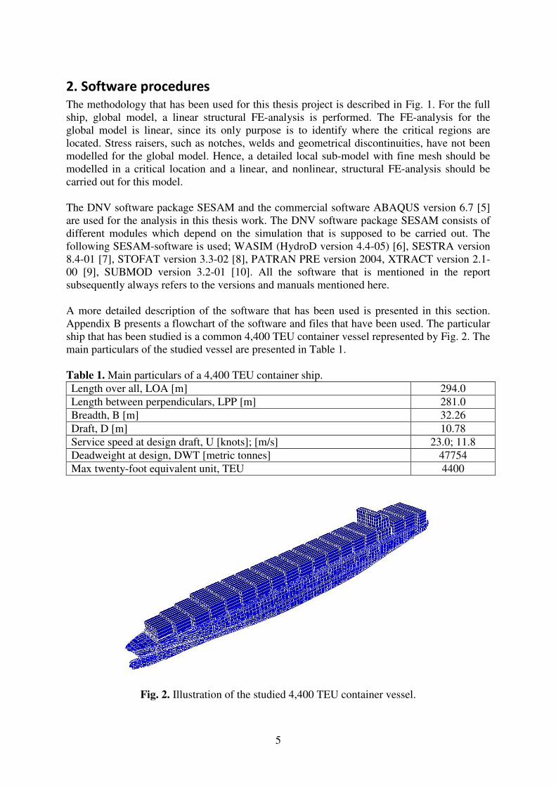
The methodology that has been used for this thesis project is described in Fig. 1. For the full ship, global model, a linear structural FE-analysis is performed. The FE-analysis for the global model is linear, since its only purpose is to identify where the critical regions are located. Stress raisers, such as notches, welds and geometrical discontinuities, have not been modelled for the global model. Hence, a detailed local sub-model with fine mesh should be modelled in a critical location and a linear, and nonlinear, structural FE-analysis should be carried out for this model. The DNV software package SESAM and the commercial software ABAQUS version 6.7 [5] are used for the analysis in this thesis work. The DNV software package SESAM consists of different modules which depend on the simulation that is supposed to be carried out. The following SESAM-software is used; WASIM (HydroD version 4.4-05) [6], SESTRA version 8.4-01 [7], STOFAT version 3.3-02 [8], PATRAN PRE version 2004, XTRACT version 2.1-00 [9], SUBMOD version 3.2-01 [10]. All the software that is mentioned in the report subsequently always refers to the versions and manuals mentioned here. A more detailed description of the software that has been used is presented in this section. Appendix B presents a flowchart of the software and files that have been used. The particular ship that has been studied is a common 4,400 TEU container vessel represented by Fig. 2. The main particulars of the studied vessel are presented in Table 1. Table 1. Main particulars of a 4,400 TEU container ship.

Length over all, LOA [m] 294.0

Length between perpendiculars, LPP [m] 281.0

Breadth, B [m] 32.26

Draft, D [m] 10.78

Service speed at design draft, U [knots]; [m/s] 23.0; 11.8

Deadweight at design, DWT [metric tonnes] 47754

Max twenty-foot equivalent unit, TEU 4400

Fig. 2. Illustration of the studied 4,400 TEU container vessel.

6

2.1. Hydrodynamic simulations

The hydrodynamic simulation has been carried out in WASIM. The simulation is performed for a ship that operates between Europe and North America during the winter season (December to March). In the hydrodynamic analysis it is assumed that the speed of the ship is a constant 23 knots. According to WASIM, the software for the fatigue analysis of the full-ship model requires the wave loads to be described in the frequency domain. For a frequency domain analysis, a Pierson-Moskowitz spectrum with 19 frequencies and 24 wave directions - heading angles - are chosen. The significant wave height is 1.0 m for the frequency domain analysis according to recommendations from DNV. Loads from a time domain analysis in WASIM is used for the linear structural FE-analysis in SESTRA for the local sub-model. The time domain analysis is performed with two significant wave heights, Hs = 6.0 m and Hs = 7.5 m. Significant wave heights that are higher than 7.5 m have not been studied, since the occurrence probability is very low for waves that are higher than 7.5 m.

2.2. Structure response analyses: linear and nonlinear

The linear structural FE-analysis for the full-ship model is performed in SESTRA. Three different analyses are performed for the detailed local sub-model. First, a linear structural FE-analysis was performed in SESTRA followed by a linear structural FE-analysis in ABAQUS. Finally, a nonlinear structural FE-analysis was preformed in ABAQUS in order to find out the amount of plastic deformation. The mesh for the global model and local sub-model was created in PATRAN PRE. The global model consists of 16980 4-node quadrilateral and 4858 3-node triangular thin shell elements. The local sub-model was created by Balatsos [3]. The local sub-model consists of 10850 8-node quadrilateral and 30 6-node triangular thin shell elements. The mesh size for the global model is about 3.0 m and for the local sub-model it is t x t, close to stress-raisers, and 50 x 50 mm in other locations. The main particulars for the global model are presented in Table 1 and the dimensions for the local sub-model are presented in Table 5. The hydrodynamic analysis was performed for the full-ship model in WASIM. The hydrodynamic simulation gives the pressure variations from the wave loads that act on the ship. These pressure variations are directly transferred from WASIM to SESTRA. SESTRA is used for linear structural FE-analysis and the structure response due to wave loading can be obtained. The result from the linear structural FE-analysis in SESTRA is post-processed in the postprocessor XTRACT. The load transfer between different levels of models was done using the sub-modelling facility SUBMOD. Figure 3 presents the local sub-model in contrast to the full ship (global model). The displacements from the full-ship analysis in SESTRA were transferred to the intermediate local model and detailed local model as boundary node displacements in SUBMOD. By using the sub-modelling technique it is possible to obtain the nodal displacements in six degrees of freedom for every node in the boundary region of the local sub-model.

7

Fig. 3. Sub-modelling from full-ship model to intermediate model to detailed local model [3]. The structural FE-analysis in SESTRA can only be used for linear structural FE-analyses. To be able to perform a nonlinear structural FE-analysis, as needed for this thesis project, ABAQUS is used as solver. The features given by SESAM, for example the boundary displacements, are used in the nonlinear structural FE-analysis in ABAQUS. The boundary displacements are implemented in an ABAQUS-script. The script works as an interface between two different solvers, SESTRA and ABAQUS, and the opportunity to change between linear and nonlinear FE-analysis in ABAQUS. The change between linear and nonlinear structural FE-analysis is dependent on the material behaviour, which is discussed in Section 3. The script that has been created for the nonlinear structural FE-analysis in ABAQUS consists of four parts:

• Mesh of the local sub-model given from PATRAN PRE.

• Material modelling for the nonlinear material behaviour.

• Surface pressure loads from internal ballast and external seawater pressure.

• Boundary displacements from the global model to the local sub-model given from SUBMOD.

8

2.3. Fatigue evaluation

The spectral fatigue analysis for fatigue damage calculation of welded plates and shells was performed in STOFAT. STOFAT obtains the principal stresses from SESTRA and calculates the accumulated partial damage [8]. The accumulated partial damage is weighted over sea states and 24 wave directions. The wave directions that are considered are 0, 15 up to 360 degrees. The definition of the wave direction, or heading angle, is presented in Fig. 4.

Fig. 4. Definition of the wave direction (heading angle) in this investigation. The container ship is designed to operate for 20 years in service and is assumed to be in full load condition in 85 per cent of the operational time. The wave climate is represented by a scatter diagram which represents the North Atlantic. Hence, a Pierson-Moskowitz wave spectrum is used and cos2 is the wave-spreading function. DNVC-I [4] for welded joints is used as a stress-life curve, also called SN-curve.

Head 180°

Starboard

Bow 135°

Starboard

Beam 90°

Starboard

Quarter 45°

Following 0°

Port Bow

225°

Port Beam

270°

Port Quarter

315°

9

3. Constitutive material modelling and data

The material behaviour is represented in ABAQUS by a constitutive material model. The material has to behave elastically in order to perform a linear structural FE-analysis. In ABAQUS, an elastic material behaviour can be modelled with Young’s modulus and Poisson’s ratio. These parameters are described in Table 2. The material needs to account for elastic-plastic behaviour for a nonlinear structural FE-analysis. For the elastic-plastic behaviour, there are several constitutive material models depending on the hardening procedure of the material. There are three models available to describe the strain hardening procedure of metals in ABAQUS. These are; isotropic hardening, kinematic hardening and combined hardening. Combined hardening is the hardening procedure that is used for this study. The combined hardening is a nonlinear hardening model, which associates the properties from both an isotropic hardening and a nonlinear kinematic hardening [11]. In order to define this material model in ABAQUS, a stress-strain curve is obtained in Fig. 5. The stress-strain curve in Fig. 5 is obtained from the Ramberg-Osgood relationship [2] and represents mild steel. The material properties for this mild steel are presented in Table 2. Table 2. Material properties for cyclic stress-strain curves [4].

Yield strength [MPa] 277

Young’s modulus, E [GPa] 210

Poisson’s ratio 0.3

Material coefficient, H’ [N/mm2] 602.8

Material coefficient, n’ 0.117

0 2 4 6 8 100

50

100

150

200

250

300

350

400

450

500

Strain, ε [%]

Str

ess,

σ [M

Pa]

Fig. 5. A half-cycle stress-strain curve for mild steel.

10

3.1. Different modes of material response

In this section, the different modes of material response due to cyclic loading from waves are described. The cyclic behaviour can be achieved by implementation of combined hardening in ABAQUS. From a cyclic load analysis in ABAQUS, the material response is obtained as a stress-strain curve. The material response can behave in four different modes; pure elastic, elastic shakedown, plastic shakedown or plastic shakedown followed by ratchetting. The different modes of material responses are presented in Fig. 6.

Fig. 6. Different modes of material response; elastic response (a), elastic shakedown (b), plastic shakedown (c) ratchetting (d) [12].

The different modes of material responses presented in Fig. 6 require some further explanation:

• Elastic response means that the material will deform elastically and return to its original shape in an unloading condition.

• Elastic shakedown is obtained when the load does not exceed the elastic shakedown limit. This occurs when a tensile load is removed and the yielded material around the plastic zone attempts to recover its original shape. When it attempts to recover its original shape, it forces the yielded material into compression and other regions away in tension. There will be a redistribution of stress that sums to zero, as required by equilibrium, and elastic shakedown is achieved [2]. In case of elastic shakedown, a stress-based approach is appropriate to use.

• Plastic shakedown is obtained when the load exceeds the elastic shakedown limit. The loop becomes stabilized with no net accumulation of plastic strain. In case of plastic shakedown, a strain-based approach is appropriate to use.

• Ratchetting occurs when further plastic flow takes place. The result is an incremental loop and the material accumulates a net strain during each cycle.

11

3.2. Kinematic and isotropic strain hardening

In this section, kinematic and isotropic strain hardening is described. These hardening models are necessary in order for the material to deform plastically. The material response when a cyclic load is applied is described in Section 3.1. The material response gives a hint of which fatigue assessment is appropriate to use. The material model has to take into account strain hardening behaviour when the load exceeds the yield stress. The combined hardening model that is used in ABAQUS takes into account both kinematic and isotropic strain hardening behaviour. Figure 7 presents the von Mises yield surface and the difference between kinematic and isotropic hardening. The axes represent the principle stresses in 2-dimensions [13] [14].

Fig. 7. Von Mises yield surface for isotropic (left) and kinematic hardening (right), where the

axes represent the principal stresses in 2-dimensions [14]. Isotropic hardening is illustrated in Fig. 7 (left). It indicates that the yield surface increases outwards from the origin. The kinematic hardening described in Fig. 7 (right) shows that the yield surface is kept constant, but its origin moves in “stress-space”. The dashed line in Fig. 7 is the yield surface and plastic deformation occurs when the stress exceeds this surface. In this study, a combined hardening model is chosen, which allows for both the size and position of the yield surface to change.

13

4. Linear finite element and fatigue analysis of full ship model

The software for fatigue analysis, STOFAT, needs the wave loads to be described in the frequency domain [6]. The wave loads are calculated in the frequency domain in the software for hydrodynamic simulation, WASIM. The ship is assumed to operate in the North Atlantic, between Europe and North America, during the winter season (December to March). Hence, a wave scatter diagram for the North Atlantic provided by DNV [4] is used. The hydrodynamic analysis and fatigue analysis assumes the service speed to be a constant 23 knots. The wave loads calculated in the frequency domain are transferred from WASIM to the linear FE-software, SESTRA, which obtains the structure response due to wave loading. STOFAT obtains the principal stresses from SESTRA and calculates the accumulated partial damage - the usage factor. The SN-curve - the stress-life curve - that is used for the fatigue analysis is DNVC-I. The SN-curve is used for welded joints and the parameters for this curve is presented in Table 3 (where N = number of cycles to failure for stress range, log a = intercept of N-axis by SN-curve, and m = negative inverse slope of the SN-curve [4]). The vessel is assumed to be in service for 20 years. The ship will be in a full load condition in 85 per cent of the time in service. Table 3. Parameters for SN-curve of welded joints [4].

N log a m

≤ 107 12.164 3.0

≥ 107 15.606 5.0

A full-ship model, i.e. global model, is used for linear structural FE-analysis in SESTRA and a fatigue analysis in STOFAT is used to identify critical locations. A critical location is defined as a location where the fatigue damage, i.e. usage factor, is high. The usage factor is defined as the design life - life in service - divided by the calculated fatigue life. For example, if the usage factor is 1.0, it will result in failure after 20 years, or if the usage factor is 0.5, it will result in failure after 40 years. The fatigue evaluation is based on analysis with stress-concentration factors. A stress-concentration factor (SCF) is the ratio between the local stress, which is the increased stress caused by a notch or weld, and the nominal stress. A better explanation of the stress-concentration factor is presented in Section 1.2. Stress-concentration factors are used for the global model in order to take into account stresses that would be caused by geometric discontinuities and welds if they would have been modelled, which they are not, since the mesh is too coarse. Stress-concentration factors are not necessary in case of local models with fine mesh since notches, welds and cut-outs have already been modelled. The stress-concentration factors that are used in the fatigue analysis are presented in Table 4 [6]. Table 4. Stress-concentration factors (SCF) [6].

Geometric stress concentration 1.0

Weld stress concentration 1.5

Eccentricity stress concentration 1.0

The positions of the boundary conditions in the global model are presented in Fig. 8. Point A has fixed translation in all directions, point B in the y-direction and point C in the y- and z-

14

directions. Hence, a linear structural FE-analysis will give numerical errors in points A, B and C. The numerical errors are taken into consideration in this study.

Fig. 8. Boundary conditions for global model.

4.1. Results from fatigue analysis

A fatigue analysis with equal probability, 0.04167 per cent, for all wave directions is performed in STOFAT. The fatigue analysis is performed in order to find critical locations in the ship. STOFAT calculates the usage factor for the full ship (global model). The wave directions 0, 15 up to 180 degrees are studied. See Fig. 4 in Section 2.3 for a definition of the wave direction. The fatigue-critical locations are presented in Fig. 9 for a fatigue analysis with equal probability for all wave directions. Figure 9 shows that the fatigue-critical regions are located in the midshipshatch corners, engine room bulkhead and in the bilge region. However, the fatigue analysis software will underestimate the fatigue-critical locations that are affected by Vlasov torsion such as, for example, those elements that are located in the bilge region. The longitudinal stresses from the vertical and horizontal bending moment are, according to Li [1], incorporated in the fatigue analysis. The influence from warping behaviour from Vlasov torsion is often disregarded. The interest in studying the maximum usage factor as a function of one wave direction was driven by the assumptions that the ship will encounter all wave directions equally many times during the ship’s service life. In this fatigue analysis, one wave direction at a time is studied and the probability for the studied wave direction is defined to 100 per cent. The wave directions from 0, 30 up to 180 degrees are studied. The sea states are described in the scatter diagram for the North Atlantic according to DNV [4]. The SN-curve for welded joints is used and the parameters are presented in Table 3. The fatigue analysis is calculated for a container ship in service for 20 years. The stress-concentration factors are presented in Table 4. The locations of the most critical elements in terms of usage factors are presented in Fig. 10. The usage factor as a function of wave direction for six critical elements is presented in Fig. 11. Figures 10 and 11 are based on the data given in Tables A1-A7 in Appendix A. The Tables A1-A7 in Appendix A present the elements with the maximum usage factors for different wave directions and the calculated fatigue life for these elements. It seems reasonable that the elements that have the maximum usage factors are located in the forward engine room bulkhead for a wave direction of 120 degrees, since the engine room is the maximum loaded region of the ship. The elements that have the maximum usage factors are located in the midships hatch corners due to the vessel’s open cross-sections. The bilge region is not among the critical elements in Fig. 10, since the influence from the warping behaviour in Vlasov torsion is often disregarded. Hence, the usage factor in the bilge region is underestimated.

15

Fig. 9. Critical regions in the ship with maximum usage factors located in the midships hatch

corners (3.8), engine room bulkhead (3.7) and in the bilge region (0.5).

Fig. 10. Critical elements with maximum usage factors and their locations in the ship.

Corners of engine

room bulkhead

Midships hatch

corners

Midships hatch corners: ~3.8

Corners of engine room

bulkhead: ~3.7

Midships hatch corners: ~3.8

Midships bilge region: ~0.5

Above

Below

Usage factor

1.0

0.91

0.82

0.73

0.64

0.55

0.46

0.36

0.27

0.18

0.09

0.0

16

0 20 40 60 80 100 120 140 160 1800

0.5

1

1.5

2

2.5

3

3.5

4

Wave Direction [degrees]

Usa

ge

Fa

cto

r

30122

11970

30177

12044

4183

22229

Fig. 11. Usage factor as a function of wave direction for critical elements (where following sea = 0 degrees and head sea = 180 degrees).

4.2. Results from stress response analysis

The linear structural FE-analysis is performed in order to identify the regions in the ship that have the highest structure response. These regions could be different from those regions with a high usage factor. The wave load analysis is done in frequency domain and is transferred as structural loads to SESTRA. The significant wave height is 1.0 m for the frequency domain analysis and is based on recommendation from DNV. The maximum von Mises stress for an element is based on one frequency (there exist 19 frequencies as described in Section 2.2). It is the frequency that will give the maximum von Mises for one wave direction. It is not obvious if the internal pressure will affect the structure response. The effect from internal ballast pressure is studied for the global model. Figure 12 presents the location of internal ballast pressure that is modelled in the wing-ballast tank. The wing-ballast tank is 13.0 m high and is located 4.4 m from the baseline. Equation 1 represents how the internal ballast pressure is modelled in the global model.

( ) ( )'4.1781.9100010 ZzzgP −××=−= ρ (1)

A linear structural FE-analysis is done with the added internal ballast pressure. The elements that are compared and their locations in the ship are presented in Fig. 13. An effect on the von Mises stress is only found for following sea with a 0 degree heading angle, see Tables A15-A16 in Appendix A. For other wave directions there is no difference in von Mises stress, see Tables A17-A22 in Appendix A. The results from the fatigue analyses are presented in Tables A23 and A24 in Appendix A.

17

The elements with maximum von Mises stress are compared and presented in Tables A8-A14 in Appendix A. The locations of the elements with maximum von Mises in the ship are presented in Figs 14 and 15. The elements in the boundary region are not used for FE-analysis due to numerical error, for example those elements in points A, B and C as described in Fig. 10. Figure 14 presents that the maximum von Mises stress will occur in the hatch corners for wave directions of 30 and 60 degrees. Figure 15 shows that the maximum von Mises stress occurs in the centre of the most forward bulkheads for wave directions of 90, 120, 150 and 180 degrees. The von Mises stresses are very low, since the structure response from only one frequency can be considered in a frequency domain analysis. It is the frequency that gives the maximum von Mises stress for each wave direction that is considered. The von Mises stress would increase if the stress from each frequency is summed, since the structure response consists of a sum of frequencies. The wave load is a sum of frequencies that are in different phases relative to each other. The von Mises stress is not scaled with local stress-concentration factors. The attempt in this study is to compare the difference between the highest fatigued region, and the highest stressed region. For this reason, there is no need to scale the von Mises stresses. The von Mises stress as a function of wave direction, for the elements with the maximum usage factor, is presented in Fig. 16. The maximum von Mises as a function of wave direction, for elements with maximum von Mises stress, is presented in Fig. 17.

Fig. 12. Region between two bulkheads where the internal ballast pressure is applied.

The internal pressure is modelled

in between these two bulkheads

18

Fig. 13. The elements located in the internal pressure region and their position in the ship.

Fig. 14. Elements with maximum von Mises stress in the internal ballast region for a wave direction of 0 degrees, and in hatch corners for wave directions of 30 and 60 degrees.

Internal ballast region: 0°

Midships hatch corners: 30° and 60°

19

Fig. 15. Elements with maximum von Mises stress in forward bulkheads and in engine room bulkheads for wave directions of 90, 120, 150 and 180 degrees.

0 20 40 60 80 100 120 140 160 1800

5

10

15

20

25

30

35


vo

n M

ise

s [

MP

a]

30122

11970

30177

12044

4183

22229

Fig. 16. Von Mises stress as a function of wave direction for elements with maximum usage factor (where following sea = 0 degree and head sea = 180 degrees).

Forward bulkhead: 90°, 120°, 150° and 180°

Engine room bulkhead: 90°, 120°, 150° and 180°

20

0 20 40 60 80 100 120 140 160 1800

5

10

15

20

25

30

35

40

45

50


Maxim

um

von M

ises [M

Pa]

6845

5238

9591

27692

29001

10901

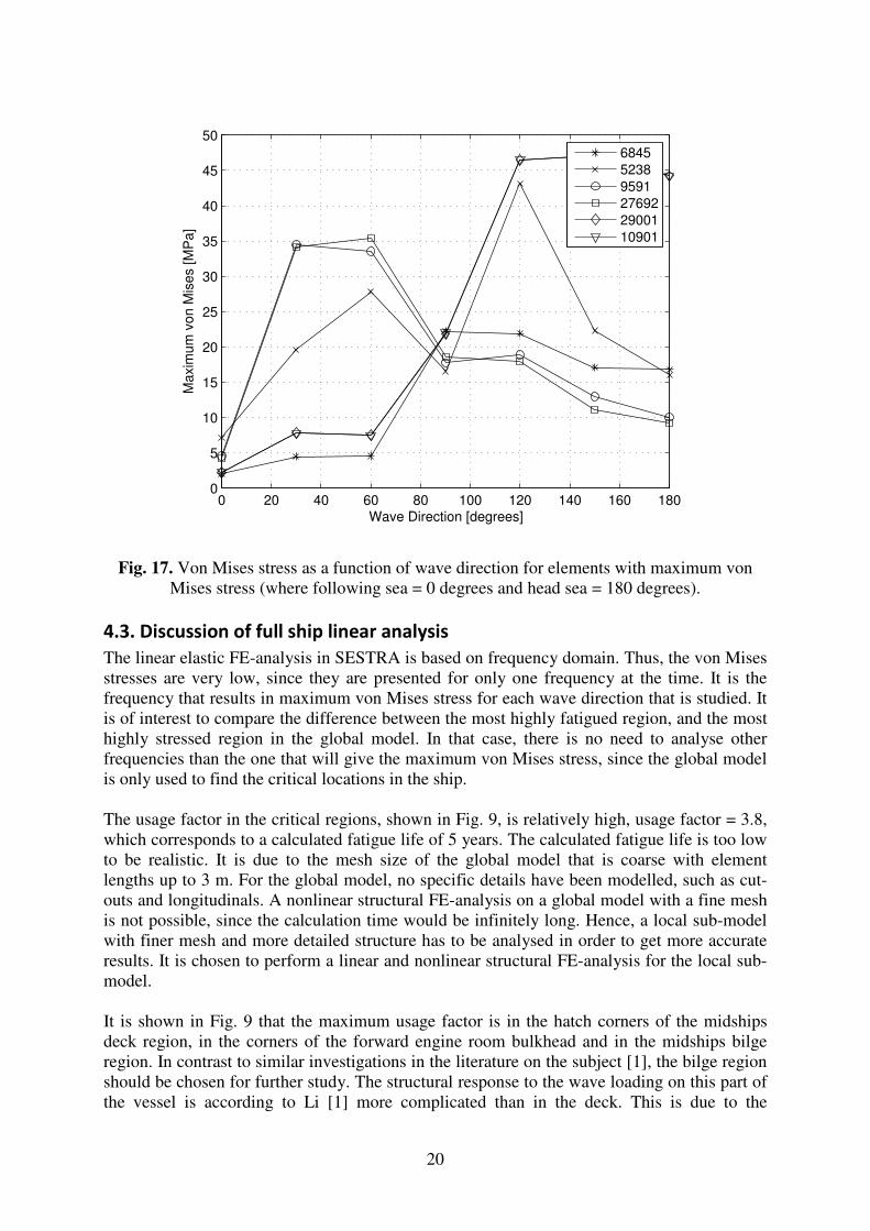
Fig. 17. Von Mises stress as a function of wave direction for elements with maximum von Mises stress (where following sea = 0 degrees and head sea = 180 degrees).

4.3. Discussion of full ship linear analysis

The linear elastic FE-analysis in SESTRA is based on frequency domain. Thus, the von Mises stresses are very low, since they are presented for only one frequency at the time. It is the frequency that results in maximum von Mises stress for each wave direction that is studied. It is of interest to compare the difference between the most highly fatigued region, and the most highly stressed region in the global model. In that case, there is no need to analyse other frequencies than the one that will give the maximum von Mises stress, since the global model is only used to find the critical locations in the ship. The usage factor in the critical regions, shown in Fig. 9, is relatively high, usage factor = 3.8, which corresponds to a calculated fatigue life of 5 years. The calculated fatigue life is too low to be realistic. It is due to the mesh size of the global model that is coarse with element lengths up to 3 m. For the global model, no specific details have been modelled, such as cut-outs and longitudinals. A nonlinear structural FE-analysis on a global model with a fine mesh is not possible, since the calculation time would be infinitely long. Hence, a local sub-model with finer mesh and more detailed structure has to be analysed in order to get more accurate results. It is chosen to perform a linear and nonlinear structural FE-analysis for the local sub-model. It is shown in Fig. 9 that the maximum usage factor is in the hatch corners of the midships deck region, in the corners of the forward engine room bulkhead and in the midships bilge region. In contrast to similar investigations in the literature on the subject [1], the bilge region should be chosen for further study. The structural response to the wave loading on this part of the vessel is according to Li [1] more complicated than in the deck. This is due to the

21

significant contribution from wave-induced warping stress in addition to the stress caused by vertical bending. However, due to the lack of time reserved for this thesis, the location of the local sub-model is based on the thesis by Balatsos [3]. Hence, the local sub-model is located in the side- shell midships region on the port side of the vessel. The local sub-model will be subjected to two different sea states: a moderate sea state with a significant wave height of Hs = 6.0 m and a higher sea state with Hs = 7.5. The stress concentrations are expected to be high for the local sub-model in this location from the wave loads of a high sea state.

23

5. Linear finite element analyses of local details

For the linear structural FE-analysis, a local sub-model in the side shell region on the port side of the vessel is studied. The location of the local sub-model is based on a thesis by Balatsos [3]. Hence, it is convenient to perform the analyses on the same local sub-model as Balatsos studied. In this region of the ship, the structure is especially complex and longitudinals are modelled, which includes cut-outs that can lead to high stress concentrations. The location of the detailed local sub-model, in contrast to the global model, is presented in Fig. 3. An intermediate sub-model exists in between these two levels of models, in order to decrease the difference in mesh size between the global model and local sub-model. Figure 18 represents the detailed local sub-model that is studied in the upcoming analyses. The dimensions of the detailed local sub-model are presented in Table 5. In highly stressed regions, like for example in the cut-out, the mesh size is the same as the thickness. In other regions that are less stressed, like for example in the web frame, the mesh size can be up to 50 x 50 mm.

Fig. 18. The detailed local sub-model.

Table 5. Dimensions of detailed local sub-model.

Length, x∆ [m] 3.40

Width, y∆ [m] 2.10

Height, z∆ [m] 0.90

Below waterline [m] 3.00-3.90

Element size [mm] t x t (or 50 x 50)

Element thickness [mm] 11-17

Cut‐out

Outer side shell

surface

Inner side shell

Longitudinal

24

Two significant wave heights, Hs = 6.0 m and Hs = 7.5 m, are selected to be studied in this thesis. These significant wave heights are the most common during the winter season (December to March). Measurements show that the occurrence probability is low for waves higher than 7.5 m, which is the reason why significant wave heights above 7.5 m have not been studied. The FE-analysis, both linear and nonlinear, for Hs = 6.0 m showed a small amount of von Mises stress. Thus, the effect from the FE-analysis with Hs = 7.5 m was studied in order to obtain higher stresses.

5.1. Linear finite element analyses in SESTRA

In this study, the result from a linear structural FE-analysis in SESTRA is used. The hydrodynamic loads are given from a time-dependent linear analysis in WASIM. The vessel is operating in the North Atlantic, thus, a Pierson-Moskowitz wave spectrum is used in SESTRA. The waves are described by 19 frequencies and 135 degrees wave direction, from a bow sea. The linear FE-analysis is performed with the limitation that the ship has a constant service speed of 23 knots. The linear structural FE-analysis in SESTRA is performed during a period of 2,400 time-steps, where 1 time-step = 0.5 second. Thus, the boundary displacements are time-dependent. The time instant that gives the highest structural response is studied in this thesis, and is obtained in the stress-history from a linear structural FE-analysis. In this study, two significant wave heights, Hs = 6.0 m and Hs = 7.5 m, are studied. The contour plot from a linear FE-analysis, for Hs = 6.0 m, is presented in Fig. 19. The highest stressed region is obtained in the cut-out of the outer side shell surface. Hence, Fig. 20 illustrates the contour plot around the cut-out. It can be seen that element 11,630 suffers the most and high stresses are locally active. The stress-history is studied, for element 11,630, and presented in terms of maximum principal stress. According to DNV [4], the maximum principal stress is considered a significant parameter when analysing fatigue-crack growth. The maximum principal stress-history from the linear FE-analysis, with Hs = 6.0 m, is illustrated in Fig. 21, where the highest response occurs in time-step 1,663. The corresponding stress-history from the linear FE-analysis, with Hs = 7.5 m, is presented in Fig. 22. The maximum principal stress occurs in time-step 2,056 and is higher than for the analysis with Hs = 6.0 m.

25

ContoursAbove4.03e+008

3.69424e+008

3.35848e+008

3.02273e+008

2.68697e+008

2.35121e+008

2.01545e+008

1.67969e+008

1.34393e+008

1.00818e+008

6.72417e+007

3.36658e+007

9000

Below

Fig. 19. Von Mises stress [Pa] for the detailed local sub-model from a linear structural FE-analysis in SESTRA, with Hs = 6.0 m.

ContoursAbove4.03e+008

3.69424e+008

3.35848e+008

3.02273e+008

2.68697e+008

2.35121e+008

2.01545e+008

1.67969e+008

1.34393e+008

1.00818e+008

6.72417e+007

3.36658e+007

9000

Below

Fig. 20. Von Mises stress [Pa] in the cut-out for the detailed local sub-model from a linear structural FE-analysis in SESTRA, with Hs = 6.0.

11629

11628

11627

11625

11626

11630

11624

26

0 500 1000 1500 20000.6

0.8

1

1.2

1.4

1.6

1.8

2

2.2

2.4

2.6

x 108

Number of time−steps

Maxim

um

princip

al str

ess,

σP

1 [P

a]

Fig. 21. Maximum principal stress in element 11630 from a linear structural FE-analysis with Hs = 6.0 m, where 1 time-step = 0.5 sec.

0 500 1000 1500 20000

0.5

1

1.5

2

2.5

3

3.5

x 108


Maxim

um

princip

al str

ess,

σP

1 [P

a]

Fig. 22. Maximum principal stress in element 11630 from a linear structural FE-analysis with Hs = 7.5 m, where 1 time-step = 0.5 sec.

27

5.2. Boundary displacements from sub-modelling - SUBMOD

Sub-modelling is used in order to obtain the boundary displacements for the detailed local sub-model. The sub-modelling technique is described in Section 2.6. A linear FE-analysis is performed for the full ship - the global model - as described in Section 5. The ship speed is 23 knots and the wave direction (heading angle) is 135 degrees. The sub-modelling technique is applied in two steps; first the loads are transferred from the global model to the intermediate sub-model, and, further, to the detailed local sub-model as described in Fig. 3. The boundary displacement from sub-modelling is given in six degrees of freedom for each time-step. A history of 2,400 time-steps is studied. The time-step that gives the highest structure response is selected. That is in time-step 1,663 for Hs = 6.0 m and time-step 2,056 for Hs = 7.5 m. The boundary displacements in these time-steps are applied in the linear, and nonlinear, FE-analysis in ABAQUS for the local sub-model. Figure 23 represents the boundary displacements in six degrees of freedom for a boundary node for Hs = 6.0 m. Figure 24 represents the boundary displacements in six degrees of freedom for a boundary node for Hs = 7.5 m. The time-step that gives the highest structure response is marked as a dotted line in Figs. 23 and 24. It is presented in Figs 23 and 24 that the torsion is severe around the x-axis. Figures 23 and 24 show that the displacement in the z-direction dominates, while the displacement in the longitudinal direction is very small.

1550 1600 1650 1700 1750−0.2

0

0.2

0.4

0.6


Tra

nsla

tion [m

]

∆x

∆y

∆z

1550 1600 1650 1700 1750

−2

−1

0

1

2

x 10−3


Rota

tion [ra

d/s

ec]

φx

φy

φz

Fig. 23. Displacements in six degrees of freedom for one boundary node for Hs = 6.0 m, where 1 time-step = 0.5 sec.

28

1950 2000 2050 2100 2150−0.2

0

0.2

0.4

0.6


Tra

nsla

tion [m

]

∆x

∆y

∆z

1950 2000 2050 2100 2150−5

0

5x 10

−3

Number of time−teps

Rota

tion [ra

d/s

ec]

φx

φy

φz

Fig. 24. Displacements in six degrees of freedom for one boundary node for Hs = 7.5 m, where 1 time-step = 0.5 sec.

5.3. Linear finite element analyses in ABAQUS

A linear FE-analysis was performed in ABAQUS and compared with the linear FE-analysis performed in SESTRA. The same mesh and material properties were used for both FE-analyses in ABAQUS and SESTRA. The material properties, Young’s modulus and Poisson’s ratio, are presented in Table 2. The mesh is presented in Fig. 18. The external sea pressure is included in the FE-analysis in SESTRA, while in ABAQUS, the effect from external sea pressure needs to be modelled. The external sea pressure is given from the linear FE-analysis in SESTRA for the local sub-model. The magnitude of the external sea pressure has to be multiplied with a factor of 4, since there are some differences between the different kinds of software. The factor of 4 is found by changing the input pressure between the analyses in ABAQUS and interpolate between the results to achieve the correct equivalent pressure. The magnitude of the pressure in SESTRA is given independently for each element. The external sea pressure in ABAQUS is simplified as distributed pressure over the surface, since the pressure does not vary that much along the studied surface. Figure 25 represents how the internal and external sea pressures are applied on the local sub-model. Table 6 shows the magnitudes of the external sea pressures that are implemented in the FE-analyses in ABAQUS for the local sub-model. The pressure from internal ballast water is also presented in the table, but it will not be included in this part of the analysis.

29

Table 6. Magnitudes of internal and external sea pressure.

Type of pressure Pressure [kPa]

Internal ballast water 102.5

External sea water (Hs = 6.0 m) 170.0

External sea water (Hs = 7.5 m) 197.0

The boundary displacements are applied on every boundary node for the detailed local sub-model as described in Fig. 26. The linear structural FE-analysis is performed with Hs = 6.0 m, and hence, the boundary displacements in time-step 1,663 are applied. The result from the linear structural FE-analysis is presented in Fig. 27.

Fig. 25. Internal (left and right inner side surface) and external (right outer side surface) sea pressure acting on the surface of the local sub-model.

Internal ballast water External sea water

30

Fig. 26. Boundary displacement applied on every boundary node in the local sub-model.

Fig. 27. Von Mises stress [Pa] around the cut-out from a linear FE-analysis in ABAQUS for

the local sub-model, with Hs = 6.0 m.

11630

11629

11628

11626

11627

11625

31

The contour plot from the linear structural FE-analysis in SESTRA, Fig. 20, is compared with the contour plot from a linear structural FE-analysis in ABAQUS, Fig. 27. The highest von Mises stress in the elements around the cut-out is presented in Table 7. Table 7. Von Mises stress from a linear structural FE-analysis in SESTRA and ABAQUS.

Element

number von Mises from SESTRA [MPa] von Mises from ABAQUS [MPa]

11624 240 310

11625 240 310

11626 220 300

11627 200 270

11628 150 210

11629 150 150

11630 250 250

The result from the linear structural FE-analysis in ABAQUS is almost identical with the result from the linear structural FE-analysis in SESTRA. Hence, the change of solver is performed properly and a further nonlinear structural FE-analysis in ABAQUS can be performed.

33

6. Nonlinear finite element analysis of local detail

The nonlinear structural FE-analysis in this study is performed in the commercial software ABAQUS. A linear structural FE-analysis performed in SESTRA and another analysis is performed in ABAQUS, as described in Section 5. A comparison between the results from the different kinds of software is also presented. The results indicate that there is good agreement between the contour plots, as shown in Figs 20 and 27, and a nonlinear structural FE-analysis can be performed. The same mesh, Fig. 18, is used for the nonlinear structural FE-analysis as for the linear structural FE-analysis in ABAQUS. Table 6 presents the magnitude of the external sea pressure and Fig. 25 shows where the pressure is applied. The modelling of the nonlinear material response is described in Section 3. In ABAQUS, a nonlinear material response for metals can be implemented as a combined, nonlinear kinematic and isotropic hardening model. The combined hardening model requires two vectors as input; the yield stress and plastic strain. The yield stress and plastic strain can be calculated by using the Ramberg-Osgood relationship [2], which uses two material parameters for mild steel, H’ and n’, that are given by DNV [4]. The values of stresses and strains that are implemented in ABAQUS are presented in Table 8. Table 8. Material properties for a nonlinear structural FE-analysis in ABAQUS.

Yield stress [MPa] Plastic strain [%]

277 0.00

278 0.13

370 1.54

400 2.96

418 4.36

432 5.77

443 7.18

452 8.60

460 10.00

603 100.00

The boundary displacements are given from the sub-modelling described in Section 2.6. The full ship, global model, has a forward speed of 23 knots. The wave direction is 135 degrees. For a nonlinear structural FE-analysis, with the significant wave height of Hs = 6.0 m, boundary displacements in time-step 1,663 are applied. For a nonlinear structural FE-analysis, with Hs = 7.5 m, boundary displacements in time-step 2,056 are applied. The time-step that is applied achieves the maximum structural response and is discussed in Section 5.2. The purpose of the upcoming analyses is to study the magnitude of the equivalent plastic strain. A description of the results from the nonlinear FE-analysis of the detailed local sub-model is given in Section 6.1. The part of interest from these simulations is the distribution and the magnitude of von Mises stress and the equivalent plastic strain in the cut-out. The cut-out on the outer side shell surface is of interest, since it is the region where the highest stress concentrations are expected due to a combination of geometric discontinuities, welds and residual stresses.

34

6.1. Nonlinear FE-analysis of local sub-model for two significant wave heights

In this study, two levels of significant wave heights are investigated, Hs = 6.0 m and Hs = 7.5 m. In this section the procedure and the results from the nonlinear structural FE-analysis for both significant wave heights are presented and compared. The mesh, external sea pressure and material model are the same for both nonlinear FE-analyses, but the boundary displacements differ depending on the significant wave height. For the nonlinear structural FE-analysis with Hs = 6.0 m, the boundary displacements are applied for time-step 1,663. Time-step 1,663 is selected according to Fig. 21, since it will result in the highest structural response. For the nonlinear structural FE-analysis with Hs = 7.5 m, the boundary displacements are applied for time-step 2,056. Time-step 2,056 is selected according to Fig. 22, since it will result in the highest structural response when the boundary displacements are applied. The part of interest is the region around the cut-out, where high stress concentrations are expected due to a combination of geometric discontinuities, welds and residual stresses. Hence, the region in the cut-out is presented in the results in Figs 28-31. Figures 28 and 29 show the results from a nonlinear structural FE-analysis with Hs = 6.0 m. The von Mises stress in the cut-out is relatively low and thus the equivalent plastic strain in the local sub-model is negligible. Only a few elements show a small quantity of plastic behaviour. The results from a nonlinear structural FE-analysis, with Hs = 7.5 m, is presented in Figs 30 and 31. The von Mises stress from a nonlinear structural FE-analysis with Hs = 7.5, Fig. 30, is higher than for Hs = 6.0 m, Fig. 28. A higher amount of stress concentrations will result in more equivalent plastic strain. A comparison between the results from the nonlinear structural FE-analyses, for Hs = 6.0 m and Hs = 7.5 m, are presented in Table 9. There are only a few elements around the cut-out where the equivalent plastic strain occurs. Thus, the position of the detailed local sub-model, in combination with the significant wave height of Hs = 6.0 m and Hs = 7.5 m, should not be considered as a strain-based region. The calculated fatigue life can be based on stress-approach. There is no need to analyse the behaviour from a nonlinear structural FE-analysis with cyclic loading. The highest structure load is already applied in the nonlinear structural FE-analysis; hence, no further plasticity will occur by analysing a cyclic load. Table 9. Von Mises stress and equivalent plastic strain for Hs = 6.0 m and Hs = 7.5 m.

Sea state Element von Mises effective

stress [MPa]

von Mises equivalent

plastic strain [%]

Hs = 6.0 m 11624 278 0.03

Hs = 6.0 m 11625 278 0.03

Hs = 6.0 m 11630 251 0.00

Hs = 7.5 m 11624 280 0.11

Hs = 7.5 m 11625 280 0.11

Hs = 7.5 m 11630 279 0.09

35

Fig. 28. Von Mises stress distribution [Pa] in the cut-out from a nonlinear structural FE-analysis in ABAQUS, with Hs = 6.0 m.

Fig. 29. Equivalent plastic strain [m/m] in the cut-out from a nonlinear structural FE-analysis, with Hs = 6.0 m.

36

Fig. 30. Von Mises stress distribution [Pa] in the cut-out from a nonlinear structural FE-analysis, with Hs = 7.5 m.

Fig. 31. Equivalent plastic strain [m/m] in the cut-out, from a nonlinear structural FE-analysis, with Hs = 7.5 m.

11624 11625

11630

37

6.2. Effect from internal and external sea pressure in high sea state

The effect of the internal ballast pressure is studied for the global model analysis, as described in Section 4.2. The results from the global analysis showed a difference in terms of stress only for following sea - a 0 degree heading angle. One may suspect that there is an error in the modelling procedure, and hence the internal pressure from ballast is modelled for the detailed local sub-model. The magnitude of the internal pressure is simplified and calculated for a full-ballast condition as in Equation 1 (where z0 is the height of the ship and z1 is the position of the local sub-model). The magnitude of the internal sea pressure is presented in Table 6. The modelling of the external sea pressure is described in Section 5.3. Figure 25 represents the surfaces of the detailed local sub-model that are affected by the pressures. Four different simulations were performed, for analysis with Hs = 7.5 m, in order to investigate how the internal and external sea pressure affects the results. The von Mises stress and equivalent plastic strain for three elements in the cut-out as described in Fig. 31 are presented in Tables 10-13. It is observed in Tables 10-13 that no plasticity will occur in the analyses in which only the internal sea pressure is applied. The internal sea pressure, which is added on both the inner and outer shell surface as presented in Fig. 25, cancels out the stresses that affect the model. The load will act in the y-direction and the stresses around the cut-out will redistribute. The worst possible case appears when only the external sea pressure is included in the analysis. Hence, the outer pressure is affecting the region around the cut-out. Table 10. Analysis without internal and external pressure.

Element von Mises effective stress

[MPa]

von Mises equivalent plastic

strain [%]

11624 253 0.00

11625 242 0.00

11630 272 0.00

Table 11. Analysis with internal pressure.


[MPa]


strain [%]

11624 180 0.00

11625 167 0.00

11630 240 0.00

Table 12. Analysis with external pressure.


[MPa]


strain [%]

11624 280 0.11

11625 280 0.11

11630 280 0.10

38

Table 13. Analysis with internal and external sea pressure.


[MPa]


strain [%]

11624 278 0.04

11625 278 0.04

11630 278 0.04

6.3. Discussion from a nonlinear FE-analysis on the local sub-model

From a nonlinear structural FE-analysis, with Hs = 7.5 m and the corresponding boundary displacements, the highest magnitude of von Mises stress is found in element 11,630. The result from such an analysis is presented in Fig. 33. Figure 30 presents the region of the cut-out in detail. The result from the nonlinear structural FE-analysis implies that high stress concentrations and high loads are acting in this region. Despite the high stress concentrations, plastic deformation does not expand that much, see Fig. 31, which indicates that the load is not high enough. It would be appropriate to refine the mesh and perform a mesh convergence test in the region in order to achieve more accurate results. Fatigue cracks could initiate and start to grow due to high stress concentrations locally in element 11,630, see Fig. 30. A welded joint exists around this region, but has not been modelled in this study. High stress concentrations could occur where there is a weld [15] [16], since welding is a high-temperature treatment. A weld would introduce tensile residual stresses that would act negatively on the fatigue resistance and life [2]. In this thesis, the modelling of welds and the inclusion of residual stresses belongs to the limitation, as described in Section 1.4. It is of interest to apply a cyclic load in the nonlinear structural FE-analysis to confirm the behaviour of the material, plastic or elastic shakedown as described in Section 3.2. Due to the fact that the stress distribution from a simulation with a static load was significantly small, an analysis with a cyclic load would only result in pure elastic shakedown. In order to obtain plastic shakedown, higher stress concentrations need to be present, i.e. the local detailed sub-model has to be moved to another location where higher stress concentrations are expected.

39

7. Conclusions

The structural response of a container vessel was analysed in this study. First, a global model - a full ship model - was studied followed by a detailed local sub-model. The fatigue analysis and the linear structural FE-analysis was performed for the global model. A linear and a nonlinear structural FE-analysis was performed for the local sub-model. A linear structural FE-analysis and fatigue analysis was performed for the global model in order to localize the critical locations. The analyses showed that the critical regions are located in the midships hatch corner, the engine room bulkhead and in the bilge region. Hence, a local sub-model should be analysed in these locations. Due to the time limitation for this thesis, local sub-models were not created for these regions. Instead, a local sub-model created by Balatsos [3] was used in order to find out if a nonlinear FE-analysis can be carried out. A study on the influence of different wave directions was performed in order to find the most critical wave direction. This study showed that the elements are affected differently depending on the wave direction. For example, the most forward elements in the region of the midships hatch corners are affected by wave directions between a 0 to 60 degrees heading angle. On the other hand, the most aft elements, for example those in the engine room bulkhead on the port side of the ship, will be mostly affected by wave directions between a 90 to 150 degrees heading angle. The side shell region on the port side of the container vessel was studied more in detail with the help of a detailed local sub-model. A linear and nonlinear structural FE-analysis was performed in ABAQUS. The results from the linear structural FE-analysis in ABAQUS were almost identical to the results from the linear structural FE-analysis that was performed in SESTRA. The linear FE-analysis indicated in higher stress concentrations than for the nonlinear structural FE-analysis in ABAQUS. Analyses with two different significant wave heights, Hs = 6.0 m and Hs = 7.5 m, were studied. The nonlinear structural FE-analysis confirmed that the highest stressed region is located in the cut-out in the outer shell of the model. However, the stresses around this region are not significantly high. The conclusion is that the local sub-model should be moved to another location where higher stresses are present. A stress-based approach can be used for the fatigue assessment for the studied local sub-model. The effect from the internal pressure from ballast was investigated for the global model and for the detailed local sub-model. Analyses were performed with and without the effect from internal ballast pressure on both levels of models in order to find out if the pressure from ballast will have an effect on the stress-level. Based on the analyses, the conclusion was that the internal pressure from ballast will have a very small impact on the stress-levels and can therefore be neglected.

41

8. Future work

There are more analyses that could have been performed if there had been more time reserved for this thesis project. This section is a recommendation for future work. Other highly stressed locations can be studied, for example in the midships bilge region on the starboard side of the ship. The accumulated fatigue damage in the midships cross section in the bilge region on the starboard side is, according to the study made by Li [1], much higher than for the port side for wave directions of 0, 45, 90, 135 and 180 degrees. Thus, the bilge region on the starboard side can be studied. Other wave directions - heading angles - can be studied. The wave direction of 135 degrees was studied for this thesis. The most critical wave direction in terms of accumulated fatigue damage is, according to Li [1], for the bilge region on the port side of the ship in a head sea – 180 degrees. In a bow sea - 135 degrees - the accumulated fatigue damage is much higher in the bilge region on the starboard side than for the bilge region on the port side. It is inconvenient to operate a container vessel from a bow sea wave direction. The complex stress pattern close to the welded joints of the local sub-models can be studied, including effects from residual and mean stresses [15, 16]. The welds have not been modelled for this project. Geometrical stress concentrations, such as cut-outs and corners in the base material, are considered. The effect of the weld can be considered since ship structures are commonly built with welded plating. Tensile residual stresses from welding will emphasize the crack-growth, which will decrease the fatigue life. A stress-based approach to fatigue for the studied local detail can be performed, as described in Appendix C. In case of further analysis in other locations, where high stress concentrations are present, a nonlinear analysis with cyclic loading can be performed followed by a strain-based fatigue life calculation.

43

9. References

[1] Z. Li (2011). Direct Calculation of Wave-Induced Loads and Fatigue Damage of Container Vessels. Licentiate thesis, Department of Shipping and Marine Technology, Chalmers University of Technology, Gothenburg, Sweden.

[2] N.E. Dowling (2007). Mechanical Behaviour of Materials. Third edition, Pearson Prentice Hall.

[3] J. Balatsos (2010). Stochastic Fatigue Assessment of a Container Vessel. MSc thesis, Department of Shipping and Marine Technology, Chalmers University of Technology, Gothenburg, Sweden.

[4] DNV [Det Norske Veritas] (2008). Classification Note No. 30.7 Fatigue Assessment of Ship Structure. October 2008, Det Norske Veritas, Hövik, Norway.

[5] Abaqus (2007). Analysis user’s manual, Version 6.7. Available online: http://abaqus.civil.uwa.edu.au/docs/abaqus/v6.7/. [Accessed: 2012-06-15].

[6] DNV [Det Norske Veritas] (2006). SESAM User Manual Wasim: Wave Loads on Vessels with Forward Speed. Version 3.4, Det Norske Veritas, Hövik, Norway.

[7] DNV [Det Norske Veritas] (2007). SESAM User Manual Sestra: Superelement Structure Analysis. Version 8.3, Det Norske Veritas, Hövik, Norway.

[8] DNV [Det Norske Veritas] (2008). SESAM User Manual Stofat: Fatigue Damage Calculation of Welded Plates and Shells. Version 3.3, Det Norske Veritas, Hövik, Norway.

[9] DNV [Det Norske Veritas] (2010). SESAM User Manual Xtract: Postprocessor for Presentation, Animation and Reporting of Results. Version 3.0, Det Norske Veritas, Hövik, Norway.

[10] DNV [Det Norske Veritas] (2004). SESAM User Manual Submod: Transfer Displacement from Global Model to Sub-Model. Version 3.0, Det Norske Veritas, Hövik, Norway.

[11] F. Sabourin and P. Simon (2005). Identification of a Combined Hardening and Application to a “One-Step” Inverse Approach. In: Proceedings of VIII International Conference on Computational Plasticity (COMPLAS VIII), E. Oñate and D.R.J. Owen (Eds), Barcelona, Spain, pp. 4

[12] J.A. Williams (1999). Wear Modelling: Analytical, Computational and Mapping: a Continuum Mechanical Approach. Wear, Vol. 225, No. 1, pp. 1-17.

[13] Autodesk Algor Simulation homepage: http://download.autodesk.com. [Accessed: 2012-06-15].

[14] Applied Mechanics of solid homepage: http://solidmechanics.org. [Accessed: 2012-06-15].

[15] L. Li, B. Zhang and T. Moan (2007). Residual Stress Shakedown in Typical Weld Joints and its Effect on Fatigue of FPSOs (OMAE2007-29285). In: Proceedings of ASME 26th International Conference on Offshore Mechanics and Arctic Engineering (OMAE2007), San Diego, California, USA, pp. 193-201.

[16] B. Zhang and T. Moan (2006). Mean Stress Effect on Fatigue of Welded Joint in FPSOs (OMAE2006-92056). In: Proceedings of ASME 25th International Conference on Offshore Mechanics and Arctic Engineering (OMAE2006), Hamburg, Germany, pp. 403-412.

A1

Appendix A: Global model calculation sheets

This Appendix contains tables with obtained general stresses and usage factors for the most critical elements in the global model.

A3

A.1. Calculation sheets for usage factors and von Mises stress

Table A1. Maximum usage factors and von Mises stress for a wave direction of 0 degrees.

Element Usage factor von Mises

[MPa]

Estimated Life

[years]

Location

30122 3.5 1.8 5.7 hatch corner (SB)

11989 3.5 1.8 5.7 hatch corner (P)

30084 3.3 2.4 6.1 hatch corner (SB)

11951 3.3 2.4 6.1 hatch corner (P)

10130 2.6 1.1 7.7 hatch corner (P)

28230 2.6 1.1 7.7 hatch corner (SB)

11970 2.6 2.1 7.7 hatch corner (P)

30103 2.6 2.1 7.7 hatch corner (SB)

12008 2.2 1.3 9.1 hatch corner (P)

30141 2.2 1.3 9.1 hatch corner (SB)



[MPa]

Estimated Life

[years]

Location

30122 3.8 7.6 5.3 hatch corner (SB)

11989 3.8 7.6 5.3 hatch corner (P)

30084 3.5 7.1 5.7 hatch corner (SB)

11951 3.5 6.2 5.7 hatch corner (P)

10130 3.0 20.5 6.7 hatch corner (P)

11970 2.9 5.9 6.9 hatch corner (P)

30103 2.7 6.5 7.4 hatch corner (SB)

28230 2.7 20.8 7.4 hatch corner (SB)

12243 2.5 45.4 8.0 hatch corner (P)

12008 2.4 6.4 8.3 hatch corner (P)



[MPa]

Estimated Life

[years]

Location

11989 3.7 5.9 5.4 hatch corner (P)

30122 3.6 6.0 5.6 hatch corner (SB)

11951 3.5 5.8 5.7 hatch corner (P)

30084 3.4 5.9 5.9 hatch corner (SB)

10130 3.0 17.8 6.7 hatch corner (P)

11970 2.9 5.3 6.9 hatch corner (P)

30103 2.6 5.4 7.7 hatch corner (SB)

28230 2.6 18.1 7.7 hatch corner (SB)

12243 2.6 33.8 7.7 hatch corner (P)

12008 2.4 5.4 8.3 hatch corner (P)

A4



[MPa]

Estimated Life

[years]

Location

4183 3.1 11.6 6.5 eng. room bulkhead (P)



11951 2.2 3.1 9.1 hatch corner (P)

11989 2.2 3.1 9.1 hatch corner (P)

30084 2.1 3.5 9.5 hatch corner (SB)

30122 2.0 3.1 10.0 hatch corner (SB)


11970 1.8 2.8 11.1 hatch corner (P)


Table A5. Maximum usage factors and von Mises stress for wave directions of 120 degrees.


[MPa]

Estimated Life

[years]

Location







22229 2.0 21.3 10.0 eng. room bulkhead (SB)

23284 1.6 29.3 12.5 eng. room bulkhead SB

30177 1.6 20.9 12.5 hatch corner (SB)

29964 1.6 21.7 12.5 hatch corner (SB)

Table A6. Maximum usage factors and von Mises stress for wave directions of 150 degrees.


[MPa]

Estimated Life

[years]

Location



30177 2.7 21.1 7.4 hatch corner (SB)

29964 2.6 20.2 7.7 hatch corner (SB)


29963 2.4 21.3 8.3 hatch corner (SB)

12044 2.3 21.1 8.7 hatch corner (P)

11830 2.3 20.8 8.7 hatch corner (P)

11831 2.3 20.2 8.7 hatch corner (P)

22229 2.2 15.1 9.1 eng. room bulkhead (SB)

A5



[MPa]

Estimated Life

[years]

Location

30177 3.2 23.0 6.5 hatch corner (SB)

12044 3.1 23.1 6.5 hatch corner (P)

29964 3.1 22.4 6.5 hatch corner (SB)

11831 3.1 22.4 6.5 hatch corner (P)

29963 3.0 23.3 6.7 hatch corner (SB)

11830 2.8 23.1 7.1 hatch corner (P)

29969 2.6 22.9 7.7 hatch corner (SB)

11836 2.6 22.9 7.7 hatch corner (P)

30173 2.6 21.5 7.7 hatch corner (SB)

29960 2.5 21.7 8.0 hatch corner (SB)

Table A8. Maximum von Mises stress for a wave direction of 0 degrees.

Element von Mises [MPa] Location

21037 21.62 internal pressure region (SB)

3854 20.95 internal pressure region (P)




1400 19.55 internal pressure region (centre)

19417 19.55 internal pressure region (centre)




Table A9. Maximum von Mises stress for wave a direction of 30 degrees.


30376 48.39 hatch corner (SB)

12243 45.39 hatch corner (P)









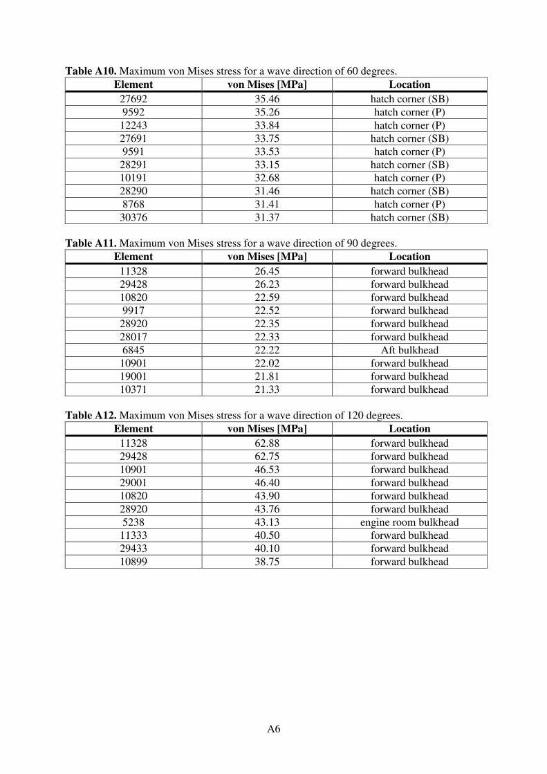
A6















11328 26.45 forward bulkhead






6845 22.22 Aft bulkhead












5238 43.13 engine room bulkhead




A7

























Table A15. The general stresses for a wave direction of 0 degrees for a ship with the effect of internal pressure.

Element SIGXX SIGYY TAUXY VON MISES

2654 4.52 6.11 -4.47 9.50

2655 8.71 10.85 -1.28 10.20

2656 9.58 11.47 0.72 10.73

2657 5.64 7.26 3.74 9.25

7423 9.11 18.81 -1.14 16.41

20671 4.53 6.10 4.48 9.50

20672 8.71 10.85 1.28 10.20

20673 9.57 11.47 -0.71 10.72

20674 5.64 7.28 -3.74 9.26

25523 9.09 18.79 1.16 16.40

A8

Table A16. The general stresses for a wave direction of 0 degrees for a ship without the effect of internal pressure.


2654 3.82 1.10 -1.47 4.25

2655 3.88 0.97 -1.33 4.19

2656 3.79 0.95 -1.18 3.98

2657 3.87 0.96 -0.83 3.77

7423 0.12 0.33 1.86 3.23

20671 3.82 1.10 1.47 4.26

20672 3.88 0.96 1.34 4.20

20673 3.79 0.94 1.18 3.99

20674 3.86 0.94 0.84 3.78

25523 0.00 0.13 -1.81 3.14

It is obvious that the internal pressure will have an effect on the general stresses for a wave direction of 0 degrees. As mentioned before, there will be no difference in general stress for the other wave directions (30, 60, 80, 120, 150 and 180 degrees). The general stresses for the other wave directions can be obtained in Tables A17-A22. Table A17. The general stresses for a wave direction of 30 degrees (the same results for a ship with and without the effect of internal pressure).


2654 22.15 7.10 -1.55 19.77

2655 22.86 7.91 -0.51 20.13

2656 -23.13 -8.32 -0.27 20.30

2657 -23.03 -8.49 -1.20 20.28

7423 15.80 6.22 -0.16 13.79

20671 -21.44 -8.32 -1.76 18.97

20672 -22.39 -9.45 -.030 19.48

20673 22.60 9.56 -0.72 19.69

20674 -21.99 -8.92 1.89 19.43

25523 -17.01 -7.66 0.04 14.75

Table A18. The general stresses for a wave direction of 60 degrees (the same results for a ship with and without the effect of internal pressure).


2654 12.80 3.33 2.01 12.01

2655 12.85 3.53 2.59 12.34

2656 -12.61 -3.63 -2.95 12.35

2657 -12.36 -3.62 -3.38 12.46

7423 -11.59 -0.70 -0.22 11.26

20671 20.61 4.85 2.78 19.28

20672 21.22 4.67 2.26 19.71

20673 21.54 4.78 1.83 19.85

20674 22.07 4.92 0.81 20.11

25523 6.84 3.20 4.86 10.30

A9



2654 -7.42 -0.78 -1.44 7.49

2655 -7.07 -0.30 -1.47 7.38

2656 -6.74 -0.19 -1.51 7.14

2657 6.83 0.33 1.67 7.28

7423 4.20 1.09 -1.25 4.35

20671 -4.90 -1.07 -1.43 5.11

20672 4.82 1.50 -1.85 5.34

20673 -5.43 -1.13 -1.32 5.46

20674 5.66 1.16 1.14 5.54

25523 3.41 3.25 -2.28 5.16



2654 -9.35 -1.43 -1.74 9.22

2655 9.47 1.17 1.86 9.50

2656 -9.81 -1.22 -1.79 9.76

2657 -10.28 -1.49 -1.99 10.22

7423 -11.62 -1.09 2.52 11.94

20671 -21.06 -5.03 -4.29 20.45

20672 21.13 4.51 4.55 20.82

20673 21.68 4.66 4.13 21.02

20674 22.46 4.89 3.04 21.13

25523 -9.25 -2.87 -6.37 13.74



2654 -5.82 -1.43 -2.52 6.83

2655 6.12 1.52 2.71 7.25

2656 -6.36 -1.56 -2.80 7.51

2657 -6.51 -1.49 -3.08 7.96

7423 -7.49 -1.43 -1.78 7.55

20671 14.22 3.14 4.07 14.73

20672 13.91 2.46 4.31 14.86

20673 14.10 2.53 4.06 14.80

20674 14.66 2.77 3.36 14.69

25523 5.32 1.13 5.21 10.25

A10



2654 6.18 1.39 -3.50 8.26

2655 6.25 1.03 -3.37 8.23

2656 5.55 0.75 -3.45 7.93

2657 5.89 0.99 -2.98 7.52

7423 -1.06 -0.14 -3.72 6.52

20671 6.19 1.38 3.53 8.31

20672 6.25 1.01 3.41 8.29

20673 5.54 0.70 3.51 8.01

20674 5.86 0.81 3.03 7.60

25523 -0.95 -0.07 3.68 6.45

Table A23. Usage factors for a set of wave directions, with the effect of internal pressure.

Element 0° 30° 60° 90° 120° 150° 180°

2654 0.37 0.21 0.15 0.07 0.04 0.05 0.14

2655 0.43 0.25 0.17 0.09 0.05 0.06 0.15

2656 0.42 0.25 0.17 0.10 0.05 0.06 0.14

2657 0.39 0.23 0.17 0.10 0.05 0.06 0.14

7423 0.09 0.08 0.08 0.05 0.03 0.02 0.01

20671 0.37 0.59 0.66 0.52 0.35 0.25 0.14

20672 0.43 0.68 0.76 0.60 0.39 0.27 0.15

20673 0.41 0.66 0.75 0.60 0.38 0.26 0.14

20674 0.39 0.63 0.72 0.57 0.37 0.25 0.14

25523 0.08 0.11 0.12 0.09 0.05 0.03 0.01

Table A24. Usage factors for a set of wave directions, without the effect of internal pressure.

Element 0° 30° 60° 90° 120° 150° 180°

2654 0.37 0.22 0.15 0.08 0.04 0.06 0.14

2655 0.42 0.25 0.17 0.09 0.05 0.06 0.15

2656 0.41 0.25 0.18 0.10 0.05 0.06 0.14

2657 0.39 0.23 0.17 0.10 0.05 0.06 0.15

7423 0.08 0.08 0.08 0.06 0.03 0.02 0.02

20671 0.37 0.59 0.66 0.52 0.35 0.25 0.15

20672 0.42 0.68 0.76 0.61 0.40 0.28 0.16

20673 0.41 0.66 0.75 0.60 0.39 0.26 0.14

20674 0.39 0.63 0.72 0.58 0.37 0.25 0.14

25523 0.08 0.11 0.12 0.09 0.05 0.03 0.01

B1

Appendix B: Program interaction

In this appendix it is explained how the different programs and files are connected together through the entire analysis of the global model and local sub-models.

B3

B.1. Flowcharts of software

The programs that have been used are the DNV software package SESAM for linear structural FE-analysis and ABAQUS for linear and nonlinear structural FE-analysis. A flowchart of the software procedure of SESAM is presented in Fig. B1 and procedure for the FE-analysis in ABAQUS is presented in Fig. B2.

Fig. B1. Flowchart of software procedure for the global model.

The various programs of the DNV software package SESAM has been used to perform the linear numerical analyses for the global model. The procedure of the analyses could be explained with the following steps:

• Create a global structural in PATRAN PRE.

• Run a hydrodynamic simulation in the frequency domain (used for wave) on the global panel model in WASIM.

• Run a hydrodynamic simulation in the time domain (used for still water) on the global panel model in WASIM.

• Run a linear FE analysis on the global structural model in SESTRA.

• Merge the results files from the frequency domain and time domain simulations into a common file in PREPOST.

• Run a long-term fatigue analysis on the global structural model in STOFAT.

• Create a local structural model in PATRAN PRE.

• Transfer the displacements from the global model to the local sub-model in SUBMOD.

• Run a nonlinear structural analysis on the local sub-model in ABAQUS (not a part of SESAM).

B4

Fig. B2. Flowchart for the nonlinear FE analysis of local sub-models. The flowchart in Figs B1 and B2 show how the programs and files are used through the entire analysis of the global model and local sub-models. The files that are created are:

• T1.FEM, which contains the finite element mesh of global model.

• L1.FEM, which contains the surface loads.

• S1.FEM, which contains the wave directions.

• R1.SIN and RI.SIF-files, which are the results files that contain the stresses and displacements.

• VTF-files, which are graphical results files used as input to the post-processor XTRACT in order to verify the usage factor.

• T11.FEM, which contains the FE-mesh of the detailed local sub-model.

• R1.SIN*, which contains the result from the global analysis.

• T11.FEM*, which contains the detailed local sub-model including the boundary displacements.

C1

Appendix C: Stress-based approach

This Appendix contains the equations and formulas for calculating the elastic stress-based approach to fatigue, also referred to as the elastic hot-spot stress approach.

C3

C.1. Stress-based approach

A methodology has been developed for fatigue assessment of ship structures by DNV, which is acknowledged as the elastic hot-spot stress approach [2]. The notion of “notch stress” and “hot-spot stress” needs some clarification before starting to explain the elastic hot-spot stress approach.

• Notch stress is the total stress at the weld toe (hot-spot location) and includes the geometric stress and the stress due to the presence of the weld.

• Hot-spot stress is the extrapolation of the structural stress at the hot-spot (weld toe) and excludes the stress due to the presence of the weld. The welds are usually not modelled in the FE-analysis.

Fig. C1. Definition of stress categories. C.1.1. Derivation of hot-spot stress

The hot-spot stress is derived by extrapolation of the structural stress at the hot-spot. Hot-spot stresses are calculated assuming linear material behaviour and using an idealized structural model with no fabrication-related misalignment. There are two procedures of deriving the hot-spot stress for modelling for a 4-node shell element with an element size between 0.5t and t: (1) A linear extrapolation of the stresses to the intersection line from the read-out points at

0.5t and 1.5t from the intersection line. The principal stress at the hot-spot is calculated from the extrapolated component values (principal stress within an angle ± 45 degrees to the normal to the weld).

(2) The hot-spot stress is taken as the stress at the read-out point 0.5t away from the intersection line and multiplied by 1.12.

C4

Fig. C2. Determination of hot-spot stress for a 4-node shell element. C.1.2. Pseudo-elastic hot-spot stress

There is an approach based on the pseudo-elastic hot-spot stress range, which is, in principle, compatible with the hot-spot strain range approach, as the total strain is converted to a pseudo-elastic stress range by using a plasticity correction factor. The plasticity correction factor is used in order to employ the S-N curve instead of a strain-cycle curve [2]. An effective pseudo stress range for calculation of low-cycle fatigue damage can be obtained as:

combeff σλσ ∆⋅=∆ (C1)

Ψ⋅= ekλ (C2)

where λ is a non-linearity correction factor, ek is a plasticity correction factor and Ψ is a

factor due to stress distribution. C.1.3. Plasticity correction factor

There are two methods of finding the pseudo linear elastic hot-spot stress: by calculating the elastic hot-spot stress obtained from linear elastic FE-analysis and using Neuber’s rule in order to obtain the actual stress in the hot-spot, and the Ramberg -Osgood relation to obtain the actual strain in the hot-spot. The second alternative is to use nonlinear FE-analysis in order to obtain the actual stress and strain directly.

elastic

pseudo

ekσ

σ= (C3)

hspseudo E εσ ⋅= (C4)

nhshs

hsKE

1

'

+=

σσε (C5)

C5

nhs

hshsnK

EK

1

2

'

1

+=

σσσσ (C6)

where elasticσ the elastic hot-spot stress is obtained from a linear elastic FE-analysis and

pseudoσ is the pseudo linear elastic hot-spot stress.

global and detailed local fatigue assessment of a...

Documents