ORIGINAL ARTICLE

Glacier response to current climate change and future scenariosin the northwestern Italian Alps

Riccardo Bonanno • Christian Ronchi •

Barbara Cagnazzi • Antonello Provenzale

Received: 25 April 2013 / Accepted: 1 August 2013

� Springer-Verlag Berlin Heidelberg 2013

Abstract We analyze longtime series of annual snout

positions of several valley glaciers in the northwestern

Italian Alps, together with a high-resolution gridded dataset

of temperature and precipitation available for the last

50 years. Glacier snout fluctuations are on average nega-

tive during this time span, albeit with a period of glacier

advance between about 1970 and 1990. To determine

which climatic variables best correlate with glacier snout

fluctuations, we consider a large set of seasonal predictors,

based on our climatic dataset, and determine the most

significant drivers by a stepwise regression technique. This

in-depth screening indicates that the average glacier snout

fluctuations strongly respond to summer temperature and

winter precipitation variations, with a delay of 5 and

10 year, respectively. Snout fluctuations display also a

significant (albeit weak) response to concurrent (same

year) spring temperature and precipitation conditions. A

linear regressive model based on these four climatic vari-

ables explains up to 93 % of the variance, which becomes

89 % when only the two delayed variables are taken into

account. When employed for out-of-sample projections,

the empirical model displays high prediction skill, and it is

thus used to estimate the average glacier response to dif-

ferent climate change scenarios (RCP4.5, RCP8.5, A1B),

using both global and regional climate models. In all cases,

glacier snout fluctuations display a negative trend, and the

glaciers of this region display an accelerated retreat, lead-

ing to a further regression of the snout position. By 2050,

the retreat is estimated to be between about 300 and 400 m

with respect to the current position. Glacier regression is

more intense for the RCP8.5 and A1B scenarios, as it could

be expected from the higher severity of these emission

pathways.

Keywords Glacier retreat � Climate change �Water

resources � Future scenarios � EC-Earth

Introduction

Mountain glaciers store a relevant portion of freshwater

resources. In the densely populated Alpine region, glaciers

are a source of freshwater for domestic, agricultural and

industrial use, and a relevant economic component for

tourism and hydro-electric power production. Modifica-

tions in the glacier storage capacity associated with climate

change can have relevant impact, as glacier melt often

supports the water supply during summer.

The front variations of Alpine glaciers show a general

trend of glacier retreat over the past 150 years, with

intermittent re-advances in the 1890s, 1920s and

1970–1980s (Patzelt 1985; Zemp et al. 2007; Calmanti

et al. 2007; Diolaiuti et al. 2012). Often, the onset of the

post-Little Ice Age retreat and the later periods of inter-

mittent re-advances in the European Alps are attributed to

changes in winter precipitation rather than temperature

(Vincent et al. 2005; Zemp et al. 2007). In the last decades,

glacier retreat in the northwestern Italian Alps has been

extremely evident, owing also to the higher temperature

rise in these mountains when compared to the global

average (Ciccarelli et al. 2008).

R. Bonanno (&) � C. Ronchi � B. Cagnazzi

Arpa Piemonte, 10135 Turin, Italy

e-mail: r.bonanno@arpa.piemonte.it

A. Provenzale

Institute of Atmospheric Sciences and Climate, CNR,

10133 Turin, Italy

123

Reg Environ Change

DOI 10.1007/s10113-013-0523-6

Climate affects glaciers through changes in mass bal-

ance, determined by the difference between accumulation

and ablation (e.g., Paterson 1994; Oerlemans 2001). Thus,

a direct way to study glacier response to climate variability

is to focus on the modifications of the glacier mass balance.

However, mass balance data are available only for a lim-

ited number of glaciers. On the other hand, records of snout

position variations are widely available, and they provide

indirect information on glacier response to climate

fluctuations.

In this work, we use snout position data and consider a

regional viewpoint, trying to assess the overall response of

glaciers in a given area to regional-scale climate variations.

When using a regional perspective, an empirical stochastic

modeling approach relating glacier snout fluctuations to

climate variability can be of value (e.g., Calmanti et al.

2007), as a substitute for detailed dynamical models of

individual glacier behavior (e.g., Jouvet et al. 2009). The

study reported here follows this approach, with the aim of

estimating the overall glacier response in the northwestern

Italian Alps to different climate change scenarios in the

coming decades.

The rest of this paper is organized as follows: In

‘‘Glaciers and climate data’’ section, we introduce the data,

and in ‘‘Glacier response to climate variability’’, section we

explore the sensitivity of Alpine glaciers to fluctuations in

precipitation and temperature. On the basis of these results,

in ‘‘An empirical model for the average glacier response’’

section, we built an empirical statistical model that relates

climatic variability to glacier snout fluctuations. ‘‘Impact of

climate change on average glacier snout fluctuations’’

section is devoted to the study of the impact of the average

response of Alpine glaciers in different climate change

scenarios. Discussions and conclusions are reported in last

section.

Glaciers and climate data

Snout position data

We analyze a set of glacier snout fluctuation data in the

western sector of the Italian Alps, in the area of Piedmont

and Valle d’Aosta. Figure 1 shows a schematic map of the

study area, indicating the locations of the 14 large glaciers

which have been monitored for several decades and have

thus been considered in our analysis.

Glacier snout data are collected by the Comitato Gla-

ciologico Italiano—Consiglio Nazionale delle Ricerche

(GCI) and regularly published in the GCI Bulletin (http://

www.glaciologia.it/). Following Calmanti et al. (2007), to

which we refer for details, we consider the mean annual

snout variation, dXji , which measures the change in the

snout position of the j-th glacier from the previous to the

current year i. To compare the behavior of different gla-

ciers, we use standardized snout fluctuations, dxji defined as:

dxji ¼

dXji � dX j

r jð1Þ

where dX jis the average snout fluctuation and r jis the

standard deviation of snout fluctuations for the j-th glacier.

All snout fluctuation data considered here cover the

period 1958–2009, while the starting date varies with the

individual glaciers. Since glacier behavior can be rather

different in the late stage of retreat, we considered only

glaciers which are presently longer than 1,500 m. For these

glaciers, even in the presence of a forecasted retreat of a

few 100 m, we can assume that the glacier length remains

large enough to justify the use of the empirical model

derived below.

Table 1 reports the main characteristics of the selected

glaciers. Almost all values of dX jare negative, confirming

the overall retreat of Alpine glaciers in this area and the

homogeneity of the regional behavior of large glaciers in

the northwestern Italian Alps (Calmanti et al. 2007). This

homogeneity allows for averaging the standardized time

series of the individual glaciers, to obtain a signal

describing the regional glacier behavior in the period

1958–2009. Before averaging the individual glacier data,

we tested for the possible presence of outliers and we

removed documented anomalies reported in the GCI bul-

letins, such as a residual snow layer at the time of mea-

surement or glacier breakup.

Figure 2 shows the average standardized glacier snout

fluctuations after removal of the documented outliers, dxi.

A 5-year running mean has been applied to the averaged

snout data to smooth out short-term fluctuations and

highlight longer-term trends and cycles.

Climatic data

The local climate in the western sector of the Italian Alps is

characterized by relatively mild winters and warm sum-

mers. The seasonal cycle is characterized by minimum

temperatures in December/January and maximum temper-

atures in July/August. Precipitation has maxima in spring

(May) and fall (November) and minima in July and January

(Regione Piemonte 1998).

Here, we use temperature and precipitation as proxies of

the whole set of climate parameters which can influence

glacier dynamics. In past years, Arpa Piemonte developed

a dataset of gridded temperature and precipitation records,

with spatial resolution 0.125�, by means of a optimal

interpolation (OI) technique (Kalnay 2003) which produces

R. Bonanno et al.

123

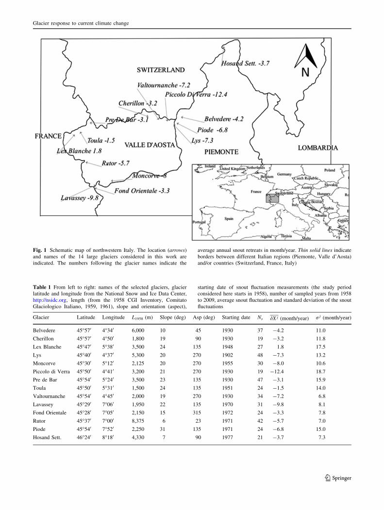
Fig. 1 Schematic map of northwestern Italy. The location (arrows)

and names of the 14 large glaciers considered in this work are

indicated. The numbers following the glacier names indicate the

average annual snout retreats in month/year. Thin solid lines indicate

borders between different Italian regions (Piemonte, Valle d’Aosta)

and/or countries (Switzerland, France, Italy)

Table 1 From left to right: names of the selected glaciers, glacier

latitude and longitude from the National Snow and Ice Data Center,

http://nsidc.org, length (from the 1958 CGI Inventory, Comitato

Glaciologico Italiano, 1959, 1961), slope and orientation (aspect),

starting date of snout fluctuation measurements (the study period

considered here starts in 1958), number of sampled years from 1958

to 2009, average snout fluctuation and standard deviation of the snout

fluctuations

Glacier Latitude Longitude L1958 (m) Slope (deg) Asp (deg) Starting date Ns dX j (month/year) r j (month/year)

Belvedere 45�570 4�340 6,000 10 45 1930 37 -4.2 11.0

Cherillon 45�570 4�500 1,800 19 90 1930 19 -3.2 11.8

Lex Blanche 45�470 5�380 3,500 24 135 1948 27 1.8 17.5

Lys 45�400 4�370 5,300 20 270 1902 48 -7.3 13.2

Moncorve 45�300 5�120 2,125 20 270 1955 30 -8.0 10.6

Piccolo di Verra 45�500 4�410 3,200 21 270 1930 19 -12.4 18.7

Pre de Bar 45�540 5�240 3,500 23 135 1930 47 -3.1 15.9

Toula 45�500 5�310 1,500 24 135 1951 24 -1.5 14.0

Valtournanche 45�540 4�450 2,000 19 270 1930 34 -7.2 6.8

Lavassey 45�290 7�060 1,950 22 135 1970 31 -9.8 8.1

Fond Orientale 45�280 7�050 2,150 15 315 1972 24 -3.3 7.8

Rutor 45�370 7�000 8,375 6 23 1971 42 -5.7 7.0

Piode 45�540 7�520 2,250 31 135 1971 24 -6.8 15.0

Hosand Sett. 46�240 8�180 4,330 7 90 1977 21 -3.7 7.3

Glacier response to current climate change

123

a spatial interpolation of the data provided by an ensemble

of meteorological stations in Piedmont and Valle d’Aosta

(Ronchi et al. 2008) for the period 1958–2009. The OI

technique consists in the assimilation of arbitrarily dis-

placed ground station data on a selected regular three-

dimensional grid map based on a background field (BF).

For temperatures, the background field is obtained by a

linear tridimensional downscaling of the ERA-40 archive

from 1958 to 2001 and of the ECMWF objective analysis

from 2002 to 2009 (for precipitation the BF is obtained

from the station raw data).

In this work, we opted for averaging the meteorological

records provided by OI analysis over a large area (the

whole Piedmont and Valle d’Aosta region) rather than

considering only the single grid point closest to the glacier

location itself (see Calmanti et al. 2007 for a detailed

discussion about this issue) obtaining a mean regional

climatic signal.

Considering standardized variables rather than raw

values helps reducing the bias due to differences in the

altitude and position of the grid points. Therefore, monthly

averages for each grid point are standardized (by sub-

tracting the mean and dividing by the standard deviation)

and then averaged over all the grid points in the study

region. The monthly data are then aggregated to provide

seasonal values. We call the seasonally averaged precipi-

tation and temperature data P(n - m) and T(n - m), where

n and m indicate the months marking the beginning and the

end of the aggregation period.

Glacier response to climate variability

Glacier snout variations respond to climatic fluctuations

with a time delay from years to tens of years (Oerlemans

2001). We estimate the value of the time lag between cli-

matic variables and glacier snout response by systemati-

cally examining the lagged cross-correlations between

individual climatic variables and snout fluctuations. To this

end, for each possible lag s (in years), we generate sys-

tematically aggregated precipitation and temperature vari-

ables covering the whole year, considering increasing

periods of aggregation (n - m) (from 3 to 6 months) and

12 possible starting months: Using precipitation as an

example, we consider Ps(1-3), Ps(1-4), Ps(1-5), Ps(1-6),

Ps(2-4), Ps(2-5), Ps(2-6), Ps(2-7), Ps(3-5) and so on.

By using this technique, we obtain 48 potential lagged

predictors for each of the two main climatic variables (12

starting months times 4 possible durations of the aggre-

gation period). Each time series is then passed through a 5-

year running average. Finally, we compute the cross-cor-

relation r between the aggregated climatic data and the

snout fluctuations dxjand estimate its significance. For each

choice of starting month and aggregation period, the esti-

mated lag between the specific climatic variable and the

glacier response is determined by the value of s associated

with the maximum cross-correlation.

The confidence level for the lagged cross-correlation

coefficient is estimated nonparametrically by employing a

Monte Carlo randomization technique. In addition, an error

bar, dr, associated at each value of r has been calculated by

a jackknife procedure (Tong 1990). These nonparametric

approaches do not require any assumption on the proba-

bility distribution of the data, and they can deal with time

series passed through a running average such as those

considered here.

Table 2 reports the values of the maximum cross-cor-

relation of precipitation (upper panel) and temperature

(lower panel) with snout fluctuations and the corresponding

lags, for each starting month and duration of the aggrega-

tion period. All cross-correlations between snout fluctua-

tions and meteorological variables have been computed in

the whole period 1958–2009.

For precipitation, all cross-correlations are significantly

different from zero, except for the variables with starting

month 4, P0(4-7)–P9(4-9). There are two main periods of

Fig. 2 Average standardized

annual snout variation for the

dataset of 14 glaciers considered

here. Error bars indicate

maximum and minimum snout

fluctuations on the ensemble of

glaciers measured in a given

year

R. Bonanno et al.

123

the year during which precipitation shows strong positive

correlation with snout fluctuations. The strongest signal

comes from the positive correlation with winter precipita-

tion ten years before the measured snout fluctuation,

P10(11-3), and it is consistent with the results of Calmanti

et al. (2007). This effect is associated with the accumula-

tion period, and the estimated lag is typical of Alpine

glaciers with the size considered here. The second is the

spring period (February–May) in the same year of the snout

fluctuation, P0(2-5). A direct effect of weather conditions

on glacier snout measurements is excluded, as snout esti-

mates are obtained in late August–early September. The

strong positive correlation for spring precipitation in the

current year (s = 0) can be interpreted by noting that

abundant spring precipitation can reduce the retreat of the

glacier front, owing to the high snow albedo that protects

the ablation region from solar radiation. On the other hand,

measurements of the snout position could be affected by

the presence of a residual snow layer which survived

summer melt, leading to estimates of the glacier length

which could be larger than the true one.

For temperature, all cross-correlations are significantly

different from zero, and the correlation coefficients are

larger than for precipitation. A period during which tem-

perature is strongly correlated with snout fluctuations is

August to January (T7(8-1), with a lag s = 7 years), and

this is presumably associated with summer ablation. The

period corresponding to the physical ablation period,

approximately from May to October (T7(5-10) in the table),

also has a good correlation with snout fluctuations. How-

ever, there are two other sub-periods which have stronger

correlations: T4(5-8), with a shorter lag s = 4 years and

T8(7-10) with a slightly larger lag.

The strongest negative correlation, however, is found for

spring temperature in the current year, T0(2-5). Higher

spring temperature could indeed favor liquid precipitation,

which tends to accelerate melting of the snow layer cov-

ering the ablation region of the glacier, while lower spring

temperatures favor precipitation in solid form. Addition-

ally, higher spring temperatures can accelerate snow melt,

resulting in a lower protection of the glacier ablation zone.

An empirical model for the average glacier response

Model construction

We introduce a linear empirical model relating N temper-

ature and M precipitation variables, defined in a given

seasonal period in each year, to the glacier snout fluctua-

tions. Since climatic data start in 1958 and some climatic

variables determine glacier snout fluctuations with a lag up

to 10 years, we use the empirical model to reconstruct

glacier fluctuations from 1968 to 2009.

Table 2 Cross-correlations between climatic variables and snout

fluctuations, as a function of the starting month on the horizontal and

of the duration of the aggregation period on the vertical. Darker colors

indicate stronger correlations, whereas light colors and white indicate

progressively weaker correlations. The upper panel is for precipita-

tion; the lower panel is for temperature. In each cell, the upper symbol

indicates the climatic variable and the lower figure is the value of the

cross-correlation (color figure online)

Precipitation

aggr

egat

ion

peri

od

3P7(1-3)

0,58P9(2-4)

0,53P0(3-5)

0,58P0(4-6)

0,22P0(5-7)

0,31P6(6-8)

0,49P6(7-9)

0,28P7(8-10)

0,20P10(9-

11) 0,26P10(10-12)

0,33P10(11-1)

0,51P10(12-2)

0,59

4P9(1-4)

0,48P0(2-5)

0,65P0(3-6)

0,52P0(4-7)

0,14P6(5-8)

0,39P9(6-9)

0,31P7(7-10)

0,29P9(8-11)

0,28P10(9-

12) 0,27P10(10-1)

0,45P10(11-2)

0,65P10(12-3)

0,63

5P0(1-5)

0,57P0(2-6)

0,57P0(3-7)

0,45P0(4-8)

0,30P9(5-9)

0,22P9(6-10)

0,33P9(7-11)

0,32P9(8-12)

0,33P10(9-1)

0,38P10(10-2)

0,64P10(11-3)

0,72P10(12-4)

0,55

6P0(1-6)

0,51P0(2-7)

0,53P0(3-8)

0,52P9(4-9)

0,13P9(5-10)

0,27P9(6-11)

0,39P9(7-12)

0,34P9(8-1)

0,39P10(9-2)

0,58P10(10-3)

0,69P10(11-4)

0,65P10(12-5)

0,50

Temperature

3T2(1-3) -0,57

T0(2-4) -0,74

T0(3-5) -0,77

T0(4-6) -0,62

T3(5-7) -0,54

T5(6-8) -0,67

T6(7-9) -0,68

T8(8-10) -0,70

T9(9-11) -0,63

T9(10-12) -0,67

T6(11-1) -0,60

T4(12-2) -0,60

4T1(1-4) -0,63

T0(2-5) -0,80

T0(3-6) -0,70

T0(4-7) -0,54

T4(5-8) -0,69

T6(6-9) -0,60

T8(7-10) -0,72

T7(8-11) -0,72

T9(9-12) -0,67

T9(10-1) -0,65

T4(11-2) -0,63

T4(12-3) -0,58

5T1(1-5) -0,71

T0(2-6) -0,75

T0(3-7) -0,60

T4(4-8) -0,66

T6(5-9) -0,64

T9(6-10) -0,62

T7(7-11) -0,71

T7(8-12) -0,72

T9(9-1) -0,72

T7(10-2) -0,65

T4(11-3) -0,61

T3(12-4) -0,65

6T0(1-6) -0,73

T0(2-7) -0,70

T4(3-8) -0,65

T5(4-9) -0,60

T7(5-10) -0,62

T7(6-11) -0,61

T7(7-12) -0,71

T7(8-1) -0,74

T7(9-2) -0,68

T7(10-3) -0,64

T4(11-4) -0,66

T3(12-5) -0,69

1 2 3 4 5 6 7 8 9 10 11 12

starting month

Glacier response to current climate change

123

The model takes the form

dxi ¼ F Tni�sT ;n

;Pmi�sP;m

n o� �þ rrWi

¼ a0 þXN

n¼1

aT ;nTni�sT;n

þXMm¼1

aP;mPmi�sP;m

þ rrWi ð2Þ

where dxiis the mean standardized snout fluctuation on year

i, averaged over all glaciers in the sample, Pmi�sP;m

and

Tni�sT ;n

are the standardized precipitation and temperature in

a given seasonal period (symbolically represented by m and

n) on years i - sP,m and i - sT,n, respectively, sP,m and sT,n

are the chosen lags for precipitation and temperature,

respectively, and for ease of notation, we have omitted the

explicit indication of the months over which the climatic

variables are averaged. The function F is the deterministic

part of the model which depends on the ensemble of cli-

matic variables, and here it is taken as a linear combina-

tion. The constant term a0 measures the long-term trend

and the coefficients aT,n and aP,m weight temperature and

precipitation dependencies, respectively. The last term is a

noise term where rr2 is the variance of the stochastic

component, and Wi is Gaussianly distributed white noise

with zero mean and unit variance (Tong, 1990). This is a

‘‘maximally random’’ version of the stochastic term that

ensures that no significant statistical structure is left out of

the model. The model residuals are then estimated as

ri ¼ dxi � F Tni�sT ;n

;Pmi�sP;m

n o� �.

The first step in the construction of the empirical model

is the choice of a proper subset of explanatory variables

among the 96 reported in Table 2. To reduce the number of

possible choices, for each starting month (i.e., for each

column in Table 2), we selected the aggregation period

which has the highest cross-correlation with snout fluctu-

ations. In some cases, cross-correlation values were very

similar, as in the case of T8(7-10), T7(7-11) and T7(7-12) in

the temperature table. In this instance, the underlying

physical process is the same regardless of the cumulating

period length. We thus got 24 variables, 12 for temperature

and 12 for precipitation, respectively.

To further reduce the number of explanatory variables,

we used a backward stepwise algorithm using the AIC

statistics (Akaike Information Criterion) for selecting the

‘‘best’’ models in the sense of explained variance and

parsimony. Applying the backward stepwise procedure to

all 24 predictors, we obtained 12 possibly relevant pre-

dictor variables: T0(1-6), T8(7-10), T3(12-5), T5(6-8), T4(5-

8), T0(2-5), P0(2-5), P6(5-8), P0(4-8), P0(1-5), P0(3-5),

P10(10-3).

To obtain an even more parsimonious model, we focused

on out-of-sample prediction. In this approach, the model

parameters are determined by means of least-square fitting

on a given portion of the data-set, and the model is then be

used to forecast the snout fluctuations in the time period

other than that used to estimate the model parameters.

To assess the combination of variables leading to the

best out-of-sample prediction, we considered all possible

combinations of the 12 significant variables identified by

the backward stepwise regression. For each combination,

we verified the ability of the linear model to perform out-

of-sample predictions, by estimating the model parameters

from the first 20 years of the available data (from 1968 to

1988, defined as the training period) and using the resulting

model to forecast glacier snout fluctuations in the second

portion of the time series, from 1989 to 2009 (verification

period). The procedure was repeated 1,000 times for each

parameter choice. We then computed the root mean

squared error RMSE and correlation coefficient r between

the average model prediction and the snout fluctuation data

in the verification period. Since a good out-of-sample

prediction should have low RMSE and high correlation r,

the models with best out-of-sample prediction ability are

those with the highest ratio between r and RMSE.

Model results

From the above analysis, the model with the best prediction

ability and lowest AIC value has the following 4 predic-

tors: P10(10-3), P0(3-5), T0(2-5) and T5(6-8). The param-

eter values for this model are reported in Table 3. The

results of the randomization test indicate that the null

hypothesis that the values of the model parameters

obtained from the least-square fit are not significantly dif-

ferent from zero must always be rejected.

The two explanatory variables that have the largest

influence in the estimation of the standardized snout fluc-

tuation are P10(10-3) and T5(6-8), followed by the less

relevant T0(2-5) and P0(3-5).

The residuals were tested to verify whether they are

normally distributed with zero mean (Tong 1990; Jacobson

et al. 2004), have constant variance across the observation

period (homoscedasticity, Breusch and Pagan 1979) and

are uncorrelated in time (Durbin and Watson 1971). The

results showed that the selected model was able to produce

residuals which passed the normality and homoscedasticity

tests. Only one time lag (at 5 years) shows a significant

residual correlation.

The upper panel of Fig. 3 shows the standardized annual

snout fluctuations and the in-sample deterministic recon-

struction (hindcast) from the selected lagged-linear model.

The lower panel of Fig. 3 shows the out-of-sample pre-

diction using the training and verification periods discussed

above.

For completeness, we have tested the behavior of a

model obtained considering only the same-year climatic

variables, T0(2-5) and P0(3-5), and of a model obtained by

R. Bonanno et al.

123

Table 3 Model parameter estimates obtained from the out-of-sample

prediction procedure. The first column indicates the predictor, the

second column reports the value of the parameter obtained by fitting

the linear model to the whole data-set, the third column reports the

95 % prediction bounds and the fourth column reports the probability

that the parameter estimate from a random reordering of the data is

larger, in absolute value, than the original parameter. Probabilities

have been estimated from a total of 1,000 random reorderings of the

time series. In the bottom of the table, R2, adjusted R2, AIC and

RMSE = rr are shown. In the lower line, the values in square

brackets refer to a model where only the delayed climatic variables

P10(10-3), T5(6-8) are used

Parameter Estimated value a 95 % prediction bounds P(ar [ |a|)

a0 0.1018 (0.0651, 0.1384) 0.

aP(10-3) 0.5714 (0.0651, 0.7728) 0.

aP(3-5) 0.1835 (-0.0035, 0.3707) 0.002

aT(2-5) -0.2732 (-0.4946, -0.0518) 0.

aT(6-8) -0.4828 (-0.6633, -0.3023) 0.

R2 = 0.93 Adjusted R2 = 0.93 AIC = -185 rr = RMSE = 0.093

[R2 = 0.90] [Adjusted R2 = 0.89] [AIC = -170.6] [rr = RMSE = 0.130]

Fig. 3 Upper panel: in-sample deterministic reconstruction of the

average annual snout variations with the selected empirical lagged-

linear model, which parameters are reported in Table 3. Confidence

bounds for the in-sample estimation are computed by including the

white noise stochastic component (reported in Eq. 2). The procedure

is repeated 1,000 times, and the uncertainty band is defined by the 5th

and 95th percentiles. Lower panel: out-of-sample prediction of the

average annual snout variation. The black solid line represents the

data, the blue solid one the in-sample estimation in the training

period, the red solid one the averages of 1,000 different out-of-sample

predictions obtained by training the stochastic linear model on the

first 21 years of data. The blue band represents the 5th and 95th

percentiles of 1,000 different forecasts

Glacier response to current climate change

123

considering only the delayed variables, P10(10-3) and T5(6-

8). While the former does not satisfactorily reproduce

glacier snout fluctuations (neither in-sample nor out-of-

sample), the model based on the delayed variables only

produces results that are substantially equivalent to those of

the full model, albeit with slightly lower statistical per-

formance. This further indicates that the main drivers of

glacier snout fluctuations are the delayed variables and that

same-year spring variables play a minor role.

Impact of climate change on average glacier snout

fluctuations

EC-Earth and RCP scenarios

The global climate change scenarios considered here are

produced by the EC-Earth model, a recent Earth system model

developed by a consortium of European research institutions

(Hazeleger 2012, see also http://ecearth.knmi.nl/).

For EC-Earth, climate change scenarios have been

simulated using the recently developed representative

concentration pathways (RCP), see Moss et al. (2010). For

this work, two RCPs were selected: a no-climate policy

high forcing scenario (RCP8.5, corresponding to 8.5 W/m2

total anthropogenic forcing in 2100) and a ‘‘stabilization

without overshoot’’ scenario (RCP4.5, corresponding to

4.5 W/m2 total anthropogenic forcing in 2100).

One advantage of the EC-Earth consortium is that, in the

framework of the international program CMIP5, several

members of an ensemble of climatic simulations have been

made available. All simulations were obtained with the

same model and the same parameterizations, and differed

simply by the choice of the initial conditions, which were

randomly extracted, after the end of the transient phase,

from a 700-year-long spin-up simulation with constant

radiative forcing at the 1,850 level. For each scenario, the

different members of the ensemble provide an estimate of

the intrinsic climate variability of the model. The different

simulations are publicly available on the ‘‘Climate

Explorer’’ Web site (http://climexp.knmi.nl/). Here, we

consider eight members of the ensemble of EC-Earth

model projections for each RCP scenario.

In order to avoid potential biases deriving by a dissim-

ilar representation of ground height between EC-Earth

climate model and the OI analysis, first we upscaled the OI

dataset to match the model horizontal resolution and then

we calculated, for each model grid point, the average dif-

ferences between the climate historical runs and the up-

scaled OI dataset during the period 1958–2009, both for

monthly mean temperature and precipitation. The results

show an average model bias of -1.8 �C and a mean model

precipitation difference ranging from -7 % to ?7 % dur-

ing Autumn and Spring. On this basis, we removed the

calculated bias from the temperatures produced by EC-

Earth for the future scenarios. No bias correction was

applied to the EC-Earth precipitation time series.

After removal of the temperature bias, the temperature

and precipitation series for each EC-Earth grid point were

standardized by using the mean and standard deviation

from the upscaled OI data in the period 1958–2009, and

used to drive the best-performing empirical glacier model

for the period 2010–2100.

Multimodel SuperEnsemble and SRES A1B scenario

The Multimodel SuperEnsemble method (Krishnamurti

et al. 1999) is based on averaging several model outputs,

which are individually weighted by an adequate set of

weights determined by comparison with observations dur-

ing a suitably defined training period. The technique first

interpolates the output of each model run on the OI grid by

bilinear interpolation. For each grid point, the multimodel

average S is defined as

S ¼ OþXN

i¼1

ai Fi � Fi

� �ð3Þ

where N is the number of models in the ensemble, ai are

weights to be determined by the procedure, Fi is the output

of the individual i-th model, Fi is the mean model value in

the training period and O is the mean of the observations in

the training period. The weights ai are obtained with a

Gauss–Jordan minimization on the difference between the

average multimodel average S and the observations O over

the whole set of grid points considered. Once the set of

weights is determined, the same weights are used to

average the model outputs in the forecast period (thus

assuming stationarity of the weights). This technique has

been applied to a large number of weather parameters in

Piedmont, with a significant reduction in forecast error

(Cane and Milelli 2006, 2010).

For our study, we used the outputs of several regional

climate models from the ENSEMBLES project for the

SRES A1B scenario runs. We use 1961–2009 as a training

period and 2010–2088 for the future scenario period (this is

the period over which the ENSEMBLES projections are

available). For the time series of temperature and precipi-

tation obtained with the Multimodel SuperEnsemble tech-

nique, bias correction is not necessary as the weights

applied to the individual model outputs are determined

explicitly to reproduce the observations in the training

R. Bonanno et al.

123

period and the model average is imposed to be equal to that

of the observations.

The average temperature and precipitation A1B Multi-

model SuperEnsemble projections were then standardized

using the mean and standard deviation from the upscaled

OI data in the training period, and used to drive the

empirical glacier model identified in the previous section

for the period 2010–2088.

Simulation of future snout fluctuations

For each scenario (and for each ensemble member in case

of EC-Earth), we generated the time series of monthly

precipitation and bias-corrected temperature, from which

we obtained the seasonally averaged signals used to drive

the glacier model. For the future projections, we adopted

the best-performing model determined in the previous

section. All the parameters of the glacier model were

estimated from the training period 1958–2009.

Figure 4 shows the standardized annual snout fluctua-

tions over the period 1958–2100, for the RCP4.5 and

RCP8.5 scenarios with the EC-Earth global model, and for

the A1B scenario with the Multimodel SuperEnsemble

approach. When different members of the EC-Earth model

ensemble are used, the uncertainty bands overlap with each

other and the colored envelope provides an indication of

the joint climatic and glacier model uncertainty for a given

scenario.

Fig. 4 Standardized annual snout fluctuations over the period

1958–2100. For each climate run, 1,000 realizations of the glacier

models were generated to provide an estimate of the uncertainty

bands, defined by the 5th and 95th percentiles of the distribution of

values produced by the glacier model. The first portion with white

uncertainty bounds refers to the training period 1958–2009 used to

determine the parameters of the glacier model; the second portion

with green uncertainty bounds refers to the simulation of the snout

variations over the period 2010–2100 (or 2088) from the climate

scenarios. Upper panel: EC-Earth for RCP8.5; middle panel: EC-

Earth for RCP4.5; lower panel: Multimodel SuperEnsemble for A1B.

The colored curves refer to the average of the glacier model runs; for

each EC-Earth scenario, eight different climate simulations with the

same model are used

Fig. 5 Snout positions in the period 1958–2100 for the three

scenarios RCP8.5, RCP4.5 and A1B. Same details as in Fig. 4

Glacier response to current climate change

123

Figure 5 shows an estimate of the cumulated snout

positions in the period 1958–2100 for the three scenarios.

To obtain the estimated glacier snout position, we con-

verted the non-dimensional standardized snout fluctuations

into dimensional values. To this end, the standardized

annual mean snout fluctuation dxi was multiplied by the

square root of the average of the variances used to stan-

dardize the glacier fluctuations in the period 1958–2009

and added to the average of the mean fluctuation of each

glacier. The snout position is always referred to the value

measured in 1968, when we start simulating the glacier

length fluctuations. For all scenarios, the results indicate a

continuing retreat of the glacier snout position.

Discussion and conclusions

In this work, we have analyzed the 1958–2009 time series

of snout fluctuations for an ensemble of fourteen large

valley glaciers in the northwestern Italian Alps, searching

for empirical correlations with the variability of tempera-

ture and precipitation recorded in this area. We have built a

best-performing empirical regressive model which relates

year-to-year snout fluctuations, averaged over the ensemble

of glaciers, to temperature and precipitation variability as

provided by a new gridded climatic data-set for the area

under study, obtained by optimal interpolation methods

from raw ground station data. The empirical model was

then driven by the temperature and precipitation data

provided by different scenarios for future climate condi-

tions, obtaining a set of ensemble predictions of the pos-

sible average response of the large glaciers considered here

to climate change in the coming decades. Such procedure

can, of course, be applied to any other mountain area where

snout fluctuation data and meteo-climatic conditions are

available.

In our approach, temperature and precipitation must be

considered as proxies for the much more complex set of

meteorological and environmental conditions which affect

glacier dynamics. Incoming solar radiation and cloudiness,

for example, can play major roles, but their direct effect was

ignored here, mainly because we were looking for a sim-

plified empirical model that uses the most commonly

available data such as temperature and precipitation. Despite

these limitations, the best-performing empirical model

derived here explains up to 93 % of explained variance.

From the analysis of the glacier and climatic data con-

sidered here, we detected a significant dependence of snout

fluctuations on summer temperatures and winter precipi-

tation, with a temporal delay of, respectively, 5 and

10 years. These delays are consistent with the earlier

results of Calmanti et al. (2007) and represent the time

taken by the climatic signal, through modifications of the

glacier mass balance, to affect the snout position. Precipi-

tation variations take a longer time to affect snout position

than temperature fluctuations, presumably owing to the

more rapid response to melting, which acts mainly on the

lower portion of the glacier, than to an increase in ice mass,

which happens mainly in the upper part of the glaciers and

requires some time to propagate to the snout.

In addition to the delayed response, we also detected a

strong and rapid (i.e., same year) response of the glacier

snout position to temperature and precipitation in spring.

Higher spring temperatures could accelerate melting of the

snow layer covering the ablation region of the glacier,

resulting in lower albedo and favoring snout retreat. Higher

temperatures also favor precipitation in liquid form, which

further contributes to the washing out of the snow layer

protecting the glacier. Instead, spring precipitation has a

positive effect, possibly due to the fact that abundant snow

precipitation in spring can increase the albedo on the lower

portion of the glacier and protect the ablation region from

solar radiation. On the other hand, a spurious effect of spring

climatic variables cannot be excluded, as snout position

measurements in late summer could be biassed by the pres-

ence of a residual snow layer, leading to a larger estimate of

the glacier length. In any case, a model including only the

two delayed variables produces results which are very sim-

ilar to those of the full four-variable model, indicating that

spring conditions do not seem to play a crucial role.

The empirical snout fluctuation model obtained from the

data analysis was then driven by the temperature and pre-

cipitation records provided by the global climate model

EC-Earth for the RCP4.5 and RCP8.5 scenarios in the

period 2010–2100, and by a Multimodel SuperEnsemble

mean of regional climate models from the ENSEMBLES

dataset, for the SRES A1B scenario in the period

2010–2088. Using several members of an ensemble of

climate simulations for EC-Earth and an ensemble of 1,000

replicates of the empirical glacier models, we were able to

provide a confidence interval for the average snout fluc-

tuations and glacier retreat expected in the coming decades.

In all cases, the glacier model indicates a strong retreat

of the glacier snouts in the northwestern Italian Alps, with

retreats between about 300 and 400 m with respect to the

current position by 2050. In general, the RCP8.5 and A1B

multimodel scenarios indicate slightly larger retreats than

RCP4.5, as could be expected from the different severity of

these emission pathways.

In the estimation of future glacier behavior, we have

used the best-performing model defined from the data

analysis, which uses a total of four explanatory variables:

summer temperature with a delay of 5 year, winter pre-

cipitation with a delay of 10 year, and same-year spring

temperature and precipitation. To provide estimates of the

maximal uncertainty associated with the imperfect

R. Bonanno et al.

123

knowledge of the proper proxies for glacier response to

climate variability, we have run the whole set of empirical

models with four explanatory variables considered in the

analysis, thus using all possible groups of four randomly

selected precipitation and temperature combinations. In

this case (not shown for the sake of conciseness), the 95 %

uncertainty bars become obviously much larger, but they

nevertheless clearly indicate significant glacier retreat by

the end of the century.

The modeling approach developed here is very simple,

and its results confirm in a rigorous way the common view

that summer temperatures and winter precipitation are

good proxies, at least in a statistical sense, of the climatic

drivers of glacier length fluctuations (see, e.g., Belloni

et al. 1985 for an early study of Italian glaciers). The fact

that a purely statistical approach quantitatively identifies

the main climatic variables affecting glacier dynamics

gives confidence in the analysis procedure and in its use for

future projections of glacier snout fluctuations. The

approach adopted here also allowed for determining the

average time delays characterizing glacier response and

indicated a possible role of same-year spring variables

which should be further analyzed in the future.

The model discussed here is appropriate for describing

the average response of (moderately) large Alpine glaciers

and can be applied whenever glacier snout fluctuations,

temperature and precipitation time series are available.

When the glaciers shrink to smaller and smaller lengths,

the model could cease to be applicable, and thus in prin-

ciple, it cannot be used to predict when glaciers will dis-

appear. For such cases, as well as for the description of

smaller glaciers, a physically based minimal model (Oer-

lemans 2011) should probably be preferred.

Acknowledgments We acknowledge useful discussions with Nic-

ola Loglisci and Renata Pelosini of ARPA Piemonte, Marco Turco of

CMCC and Sandro Calmanti of ENEA. We are grateful to Jost von

Hardenberg of CNR-ISAC for help with the EC-Earth climatic sim-

ulations and to two anonymous reviewers who helped us to improve

the presentation of the results. This work was partially funded by the

EU FP7 Integrated Project ACQWA (www.acqwa.ch) and by the

Project of Interest NextData (www.nextdataproject.it) of the Italian

Ministry for Education, University and Research (MIUR).

References

Belloni S, Catasta G, Smiraglia C (1985) Climatic parameters and

glacial fluctuations in the period 1950–1982. Geogr Fis Dinam

Quat 8:97–123

Breusch TS, Pagan AR (1979) Simple test for heteroscedasticity and

random coefficient variation. Econometrica 47:1287–1294

Calmanti S, Motta L, Turco M, Provanzale A (2007) Impact of

climate variability on Alpine glaciers in northwestern Italy. Int J

Climatol 27:2041–2053

Cane D, Milelli M (2006) Weather forecasts obtained with a

Multimodel SuperEnsemble Technique in a complex orography

region. Meteorol Z 15:207–214

Cane D, Milelli M (2010) Can a Multimodel SuperEnsemble

technique be used for precipitation forecasts? Adv Geosci

25:17–22

Ciccarelli N, von Hardenberg J, Provenzale A, Ronchi C, Vargiu A,

Pelosini R (2008) Climate variability in north-western Italy

during the second half of the 20th century. Glob Planet Chang

63:185–195

Diolaiuti GA, Bocchiola D, Vagliasindi M, D’Agata C, Smiraglia C

(2012) The 1975–2005 glacier changes in Aosta Valley (Italy)

and the relations with climate evolution. Progr Phys Geogr.

doi:10.1177/0309133312456413

Durbin J, Watson GS (1971) Testing for serial correlation in least

squares regression III. Biometrika 58:1–19

Hazeleger W (2012) EC-Earth v2.2: description and validation of a

new seamless earth system prediction model. Clim Dyn

39:2611–2629

Jacobson AR, Provenzale A, von Hardenberg A, Bassano B, Festa-

Bianchet M (2004) Climate forcing and density dependence in a

mountain ungulate population. Ecology 85:1598–1610

Jouvet G, Huss M, Blatter H, Picasso M, Rappaz J (2009) Numerical

simulation of Rhonegletscher from 1874 to 2100. J Comp Phys

228:6426–6439

Kalnay E (2003) Atmospheric modeling, data assimilation and

predictability. Cambridge University Press, Cambridge

Krishnamurti TN, Kishtawal CM, LaRow TE, Bachiochi DR, Zhang

Z, Williford CE, Gadgil S, Surendran S (1999) Improved

weather and seasonal climate forecasts from Multimodel Supe-

rEnsemble. Science 285:1548–1550

Moss RH et al (2010) The next generation of scenarios for climate

change research and assessment. Nature 463:747–756. doi:10.

1038/nature08823

Oerlemans J (2001) Glaciers and climate change. Balkema Publishers,

Lisse

Oerlemans J (2011) Minimal glacier models. Second print. Igitur,

Utrecht Publishing & Archiving Services, Universi-

teitsbibliotheek Utrecht. ISBN 978-90-6701-022-1

Paterson WSB (1994) The physics of glaciers, 3rd edn. Pergamon

Press, Oxford

Patzelt G (1985) The period of glacier advances in the Alps, 1965 to

1980. Z Gletscherk Glazialgeol 21:403–407

Regione Piemonte (1998) Distribuzione regionale di piogge e

temperature. Collana Studi Climatologici in Piemonte, vol 1

Ronchi C, De Luigi C, Ciccarelli N, Loglisci N (2008) Development

of a daily gridded climatological air temperature dataset based

on a optimal interpolation of ERA-40 reanalysis downscaling

and a local high resolution thermometers network. Dissertation,

8th EMS annual meeting & 7th European conference on applied

climatology, Amsterdam

Tong H (1990) Nonlinear time series: a dynamical system approach.

Oxford University Press, Oxford

Vincent C, Le Meur E, Six D, Funk M (2005) Solving the paradox of

the end of the Little Ice Age in the Alps. Geophys Res Lett

32:L09706. doi:10.1029/2005GL022552

Zemp M, Paul F, Hoelzle M, Haeberli W (2007) Glacier fluctuations

in the European Alps 1850–2000: an overview and spatio-

temporal analysis of available data. In: Orlove B, Wiegandt E,

Luckman B (eds) The darkening peaks: Glacial retreat in

scientific and social context. University of California Press,

Berkeley, pp 152–167

Glacier response to current climate change

123