F L U I D K I N E M AT I C S

Fluid kinematics deals with describing the motion of fluids without nec-

essarily considering the forces and moments that cause the motion. In

this chapter, we introduce several kinematic concepts related to flow-

ing fluids. We discuss the material derivative and its role in transforming

the conservation equations from the Lagrangian description of fluid flow

(following a fluid particle) to the Eulerian description of fluid flow (pertain-

ing to a flow field). We then discuss various ways to visualize flow fields—

streamlines, streaklines, pathlines, timelines, and optical methods schlieren

and shadowgraph—and we describe three ways to plot flow data—profile

plots, vector plots, and contour plots. We explain the four fundamental kine-

matic properties of fluid motion and deformation—rate of translation, rate

of rotation, linear strain rate, and shear strain rate. The concepts of vortic-

ity, rotationality, and irrotationality in fluid flows are also discussed.

Finally, we discuss the Reynolds transport theorem (RTT), emphasizing its

role in transforming the equations of motion from those following a system

to those pertaining to fluid flow into and out of a control volume. The anal-

ogy between material derivative for infinitesimal fluid elements and RTT for

finite control volumes is explained.

•

121

CHAPTER

4OBJECTIVES

When you finish reading this chapter, you

should be able to

� Understand the role of the

material derivative in

transforming between

Lagrangian and Eulerian

descriptions

� Distinguish between various

types of flow visualizations

and methods of plotting the

characteristics of a fluid flow

� Have an appreciation for the

many ways that fluids move

and deform

� Distinguish between rotational

and irrotational regions of flow

based on the flow property

vorticity

� Understand the usefulness of

the Reynolds transport theorem

cen72367_ch04.qxd 10/29/04 2:23 PM Page 121

4–1 � LAGRANGIAN AND EULERIAN DESCRIPTIONS

The subject called kinematics concerns the study of motion. In fluid

dynamics, fluid kinematics is the study of how fluids flow and how to

describe fluid motion. From a fundamental point of view, there are two dis-

tinct ways to describe motion. The first and most familiar method is the one

you learned in high school physics class—to follow the path of individual

objects. For example, we have all seen physics experiments in which a ball

on a pool table or a puck on an air hockey table collides with another ball or

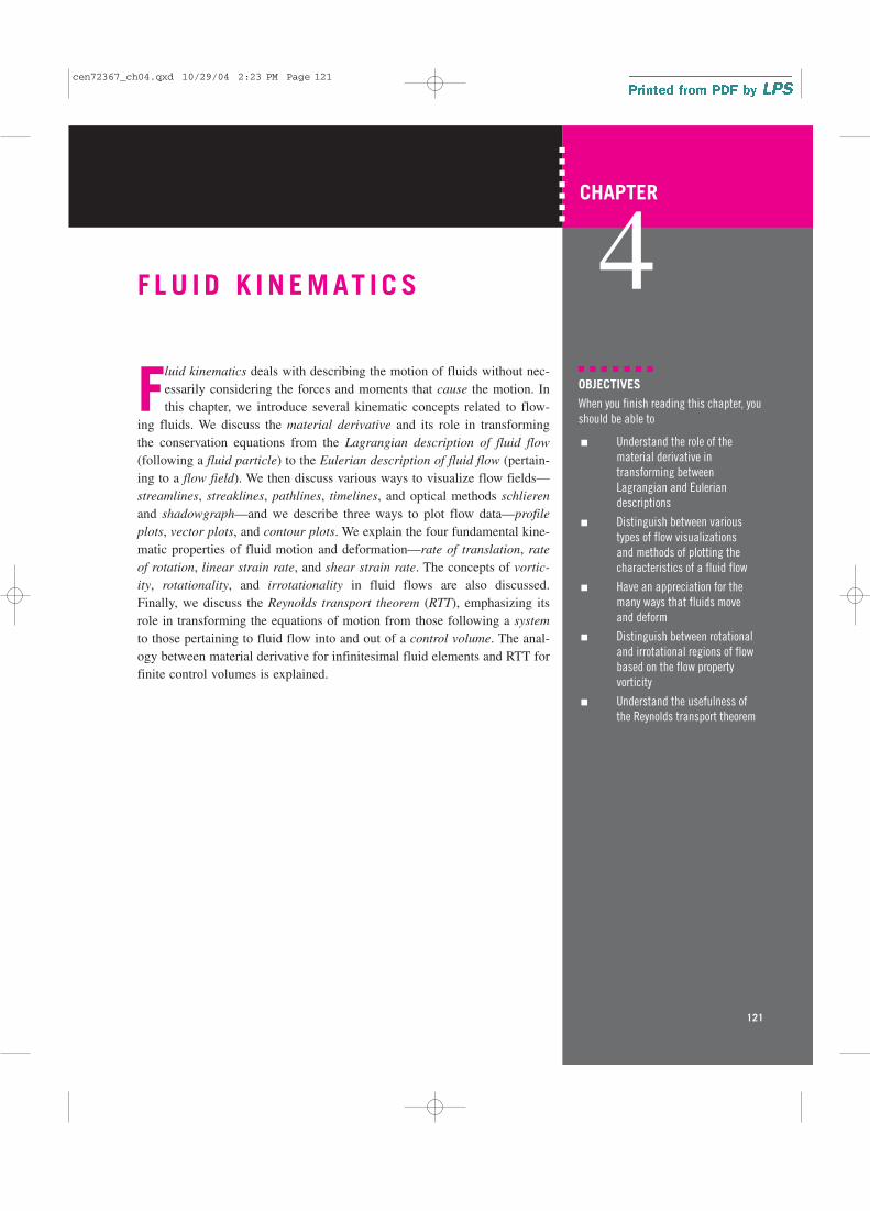
puck or with the wall (Fig. 4–1). Newton’s laws are used to describe the

motion of such objects, and we can accurately predict where they go and

how momentum and kinetic energy are exchanged from one object to another.

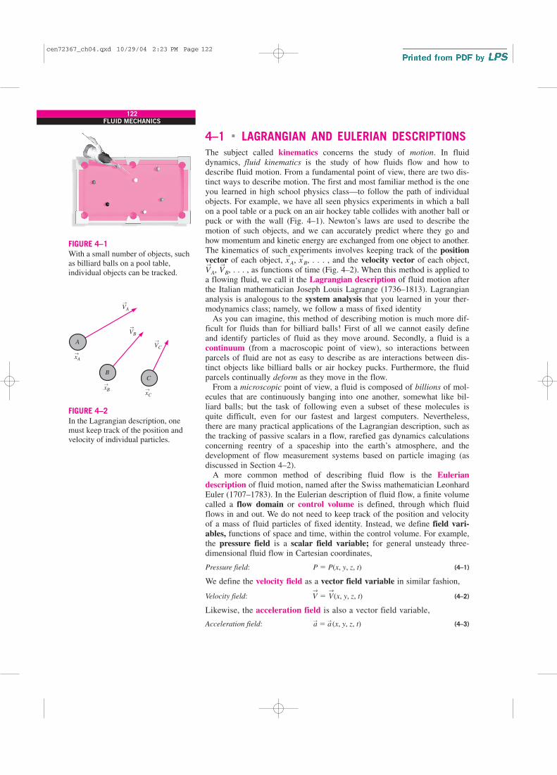
The kinematics of such experiments involves keeping track of the positionvector of each object, x

→

A, x→

B, . . . , and the velocity vector of each object,

V→

A, V→

B, . . . , as functions of time (Fig. 4–2). When this method is applied to

a flowing fluid, we call it the Lagrangian description of fluid motion after

the Italian mathematician Joseph Louis Lagrange (1736–1813). Lagrangian

analysis is analogous to the system analysis that you learned in your ther-

modynamics class; namely, we follow a mass of fixed identity

As you can imagine, this method of describing motion is much more dif-

ficult for fluids than for billiard balls! First of all we cannot easily define

and identify particles of fluid as they move around. Secondly, a fluid is a

continuum (from a macroscopic point of view), so interactions between

parcels of fluid are not as easy to describe as are interactions between dis-

tinct objects like billiard balls or air hockey pucks. Furthermore, the fluid

parcels continually deform as they move in the flow.

From a microscopic point of view, a fluid is composed of billions of mol-

ecules that are continuously banging into one another, somewhat like bil-

liard balls; but the task of following even a subset of these molecules is

quite difficult, even for our fastest and largest computers. Nevertheless,

there are many practical applications of the Lagrangian description, such as

the tracking of passive scalars in a flow, rarefied gas dynamics calculations

concerning reentry of a spaceship into the earth’s atmosphere, and the

development of flow measurement systems based on particle imaging (as

discussed in Section 4–2).

A more common method of describing fluid flow is the Euleriandescription of fluid motion, named after the Swiss mathematician Leonhard

Euler (1707–1783). In the Eulerian description of fluid flow, a finite volume

called a flow domain or control volume is defined, through which fluid

flows in and out. We do not need to keep track of the position and velocity

of a mass of fluid particles of fixed identity. Instead, we define field vari-ables, functions of space and time, within the control volume. For example,

the pressure field is a scalar field variable; for general unsteady three-

dimensional fluid flow in Cartesian coordinates,

Pressure field: (4–1)

We define the velocity field as a vector field variable in similar fashion,

Velocity field: (4–2)

Likewise, the acceleration field is also a vector field variable,

Acceleration field: (4–3)a→

� a→

(x, y, z, t)

V→

� V→

(x, y, z, t)

P � P(x, y, z, t)

122FLUID MECHANICS

FIGURE 4–1

With a small number of objects, such

as billiard balls on a pool table,

individual objects can be tracked.

VB

VC

xA

xBxC

A

BC

VA

→

→

→

→

→

→

FIGURE 4–2

In the Lagrangian description, one

must keep track of the position and

velocity of individual particles.

cen72367_ch04.qxd 10/29/04 2:23 PM Page 122

Collectively, these (and other) field variables define the flow field. The

velocity field of Eq. 4–2 can be expanded in Cartesian coordinates (x, y, z),

(i→

, j→

, k→

) as

(4–4)

A similar expansion can be performed for the acceleration field of Eq. 4–3.

In the Eulerian description, all such field variables are defined at any loca-

tion (x, y, z) in the control volume and at any instant in time t (Fig. 4–3). In

the Eulerian description we don’t really care what happens to individual

fluid particles; rather we are concerned with the pressure, velocity, accelera-

tion, etc., of whichever fluid particle happens to be at the location of interest

at the time of interest.

The difference between these two descriptions is made clearer by imagin-

ing a person standing beside a river, measuring its properties. In the

Lagrangian approach, he throws in a probe that moves downstream with the

water. In the Eulerian approach, he anchors the probe at a fixed location in

the water.

While there are many occasions in which the Lagrangian description is

useful, the Eulerian description is often more convenient for fluid mechanics

applications. Furthermore, experimental measurements are generally more

suited to the Eulerian description. In a wind tunnel, for example, velocity or

pressure probes are usually placed at a fixed location in the flow, measuring

V→

(x, y, z, t) or P(x, y, z, t). However, whereas the equations of motion in the

Lagrangian description following individual fluid particles are well known

(e.g., Newton’s second law), the equations of motion of fluid flow are not so

readily apparent in the Eulerian description and must be carefully derived.

EXAMPLE 4–1 A Steady Two-Dimensional Velocity Field

A steady, incompressible, two-dimensional velocity field is given by

(1)

where the x- and y-coordinates are in meters and the magnitude of velocity

is in m/s. A stagnation point is defined as a point in the flow field where the

velocity is identically zero. (a) Determine if there are any stagnation points in

this flow field and, if so, where? (b) Sketch velocity vectors at several loca-

tions in the domain between x � �2 m to 2 m and y � 0 m to 5 m; quali-

tatively describe the flow field.

SOLUTION For the given velocity field, the location(s) of stagnation point(s)

are to be determined. Several velocity vectors are to be sketched and the

velocity field is to be described.

Assumptions 1 The flow is steady and incompressible. 2 The flow is two-

dimensional, implying no z-component of velocity and no variation of u or v

with z.

Analysis (a) Since V→

is a vector, all its components must equal zero in

order for V→

itself to be zero. Using Eq. 4–4 and setting Eq. 1 equal to zero,

Stagnation point:

Yes. There is one stagnation point located at x � �0.625 m, y � 1.875 m.

v � 1.5 � 0.8y � 0 → y � 1.875 m

u � 0.5 � 0.8x � 0 → x � �0.625 m

V→

� (u, v) � (0.5 � 0.8x) i→

� (1.5 � 0.8y) j→

V→

� (u, v, w) � u(x, y, z, t) i→

� v(x, y, z, t) j→

� w(x, y, z, t)k→

123CHAPTER 4

Control volume

V(x, y, z, t)

P(x, y, z, t)

(x, y ,z)

→

FIGURE 4–3

In the Eulerian description, one

defines field variables, such as the

pressure field and the velocity field, at

any location and instant in time.

cen72367_ch04.qxd 10/29/04 2:23 PM Page 123

(b) The x- and y-components of velocity are calculated from Eq. 1 for several

(x, y) locations in the specified range. For example, at the point (x � 2 m, y

� 3 m), u � 2.10 m/s and v � �0.900 m/s. The magnitude of velocity (the

speed) at that point is 2.28 m/s. At this and at an array of other locations,

the velocity vector is constructed from its two components, the results of

which are shown in Fig. 4–4. The flow can be described as stagnation point

flow in which flow enters from the top and bottom and spreads out to the

right and left about a horizontal line of symmetry at y � 1.875 m. The stag-

nation point of part (a) is indicated by the blue circle in Fig. 4–4.

If we look only at the shaded portion of Fig. 4–4, this flow field models a

converging, accelerating flow from the left to the right. Such a flow might be

encountered, for example, near the submerged bell mouth inlet of a hydro-

electric dam (Fig. 4–5). The useful portion of the given velocity field may be

thought of as a first-order approximation of the shaded portion of the physi-

cal flow field of Fig. 4–5.

Discussion It can be verified from the material in Chap. 9 that this flow

field is physically valid because it satisfies the differential equation for con-

servation of mass.

Acceleration FieldAs you should recall from your study of thermodynamics, the fundamental

conservation laws (such as conservation of mass and the first law of thermo-

dynamics) are expressed for a system of fixed identity (also called a closed

system). In cases where analysis of a control volume (also called an open

system) is more convenient than system analysis, it is necessary to rewrite

these fundamental laws into forms applicable to the control volume. The

same principle applies here. In fact, there is a direct analogy between sys-

tems versus control volumes in thermodynamics and Lagrangian versus

Eulerian descriptions in fluid dynamics. The equations of motion for fluid

flow (such as Newton’s second law) are written for an object of fixed iden-

tity, taken here as a small fluid parcel, which we call a fluid particle or

material particle. If we were to follow a particular fluid particle as it

moves around in the flow, we would be employing the Lagrangian descrip-

tion, and the equations of motion would be directly applicable. For example,

we would define the particle’s location in space in terms of a material posi-tion vector (xparticle(t), yparticle(t), zparticle(t)). However, some mathematical

manipulation is then necessary to convert the equations of motion into

forms applicable to the Eulerian description.

Consider, for example, Newton’s second law applied to our fluid particle,

Newton’s second law: (4–5)

where F→

particle is the net force acting on the fluid particle, mparticle is its mass,

and a→

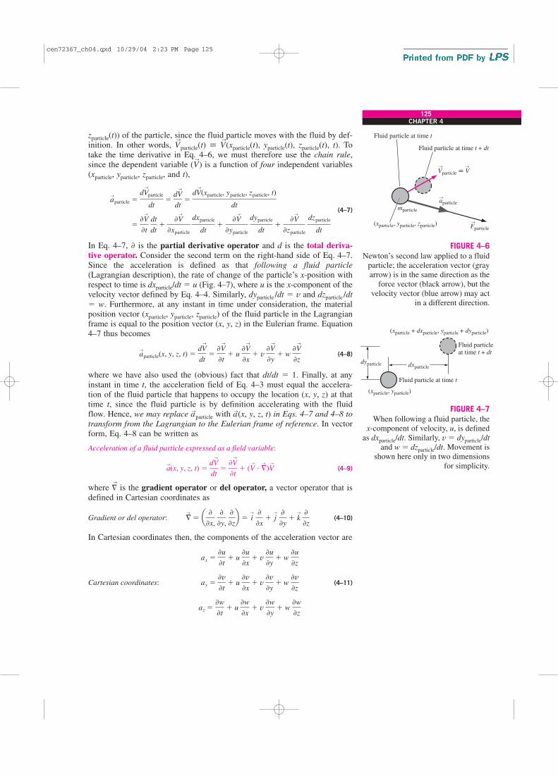
particle is its acceleration (Fig. 4–6). By definition, the acceleration of

the fluid particle is the time derivative of the particle’s velocity,

Acceleration of a fluid particle: (4–6)

However, at any instant in time t, the velocity of the particle is the same

as the local value of the velocity field at the location (xparticle(t), yparticle(t),

a→

particle �dV

→

particle

dt

F→

particle � mparticlea→

particle

124FLUID MECHANICS

Scale:

5

4

3

2y

1

0

–1

–3 –2 –1 0

x

1 2 3

10 m/s

FIGURE 4–4

Velocity vectors for the velocity field

of Example 4–1. The scale is shown

by the top arrow, and the solid black

curves represent the approximate

shapes of some streamlines, based on

the calculated velocity vectors. The

stagnation point is indicated by the

blue circle. The shaded region

represents a portion of the flow field

that can approximate flow into an inlet

(Fig. 4–5).

Region in which thevelocity field is modeled

Streamlines

FIGURE 4–5

Flow field near the bell mouth inlet of

a hydroelectric dam; a portion of the

velocity field of Example 4–1 may be

used as a first-order approximation of

this physical flow field. The shaded

region corresponds to that of Fig. 4–4.

cen72367_ch04.qxd 10/29/04 2:23 PM Page 124

zparticle(t)) of the particle, since the fluid particle moves with the fluid by def-

inition. In other words, V→

particle(t) � V→

(xparticle(t), yparticle(t), zparticle(t), t). To

take the time derivative in Eq. 4–6, we must therefore use the chain rule,

since the dependent variable (V→

) is a function of four independent variables

(xparticle, yparticle, zparticle, and t),

(4–7)

In Eq. 4–7, � is the partial derivative operator and d is the total deriva-tive operator. Consider the second term on the right-hand side of Eq. 4–7.

Since the acceleration is defined as that following a fluid particle

(Lagrangian description), the rate of change of the particle’s x-position with

respect to time is dxparticle/dt � u (Fig. 4–7), where u is the x-component of the

velocity vector defined by Eq. 4–4. Similarly, dyparticle /dt � v and dzparticle /dt

� w. Furthermore, at any instant in time under consideration, the material

position vector (xparticle, yparticle, zparticle) of the fluid particle in the Lagrangian

frame is equal to the position vector (x, y, z) in the Eulerian frame. Equation

4–7 thus becomes

(4–8)

where we have also used the (obvious) fact that dt/dt � 1. Finally, at any

instant in time t, the acceleration field of Eq. 4–3 must equal the accelera-

tion of the fluid particle that happens to occupy the location (x, y, z) at that

time t, since the fluid particle is by definition accelerating with the fluid

flow. Hence, we may replace a→

particle with a→(x, y, z, t) in Eqs. 4–7 and 4–8 to

transform from the Lagrangian to the Eulerian frame of reference. In vector

form, Eq. 4–8 can be written as

Acceleration of a fluid particle expressed as a field variable:

(4–9)

where �→

is the gradient operator or del operator, a vector operator that is

defined in Cartesian coordinates as

Gradient or del operator: (4–10)

In Cartesian coordinates then, the components of the acceleration vector are

Cartesian coordinates: (4–11)

az ��w

�t� u

�w

�x� v

�w

�y� w

�w

�z

ay ��v

�t� u

�v

�x� v

�v

�y� w

�v

�z

ax ��u

�t� u

�u

�x� v

�u

�y� w

�u

�z

§→

� a �

�x,

�

�y, �

�zb � i

→

�

�x� j

→

�

�y� k

→

�

�z

a→

(x, y, z, t) �dV

→

dt�

�V→

�t� (V

→

� §→

)V→

a→

particle(x, y, z, t) �dV

→

dt�

�V→

�t� u

�V→

�x� v

�V→

�y� w

�V→

�z

��V

→

�t dt

dt�

�V→

�xparticle

dxparticle

dt�

�V→

�yparticle

dyparticle

dt�

�V→

�zparticle

dzparticle

dt

a→

particle �dV

→

particle

dt�

dV→

dt�

dV→

(xparticle, yparticle, zparticle, t)

dt

125CHAPTER 4

Vparticle � V

Fparticle

aparticle

mparticle

(xparticle, yparticle, zparticle)

Fluid particle at time t

Fluid particle at time t + dt

→ →

→

→

FIGURE 4–6

Newton’s second law applied to a fluid

particle; the acceleration vector (gray

arrow) is in the same direction as the

force vector (black arrow), but the

velocity vector (blue arrow) may act

in a different direction.

Fluid particle at time t

Fluid particleat time t + dt

(xparticle, yparticle)

(xparticle + dxparticle, yparticle + dyparticle)

dyparticle dxparticle

FIGURE 4–7

When following a fluid particle, the

x-component of velocity, u, is defined

as dxparticle/dt. Similarly, v � dyparticle/dt

and w � dzparticle/dt. Movement is

shown here only in two dimensions

for simplicity.

cen72367_ch04.qxd 10/29/04 2:23 PM Page 125

The first term on the right-hand side of Eq. 4–9, �V→

/�t, is called the localacceleration and is nonzero only for unsteady flows. The second term,

(V→

· �→

)V→

, is called the advective acceleration (sometimes the convectiveacceleration); this term can be nonzero even for steady flows. It accounts

for the effect of the fluid particle moving (advecting or convecting) to a new

location in the flow, where the velocity field is different. For example, con-

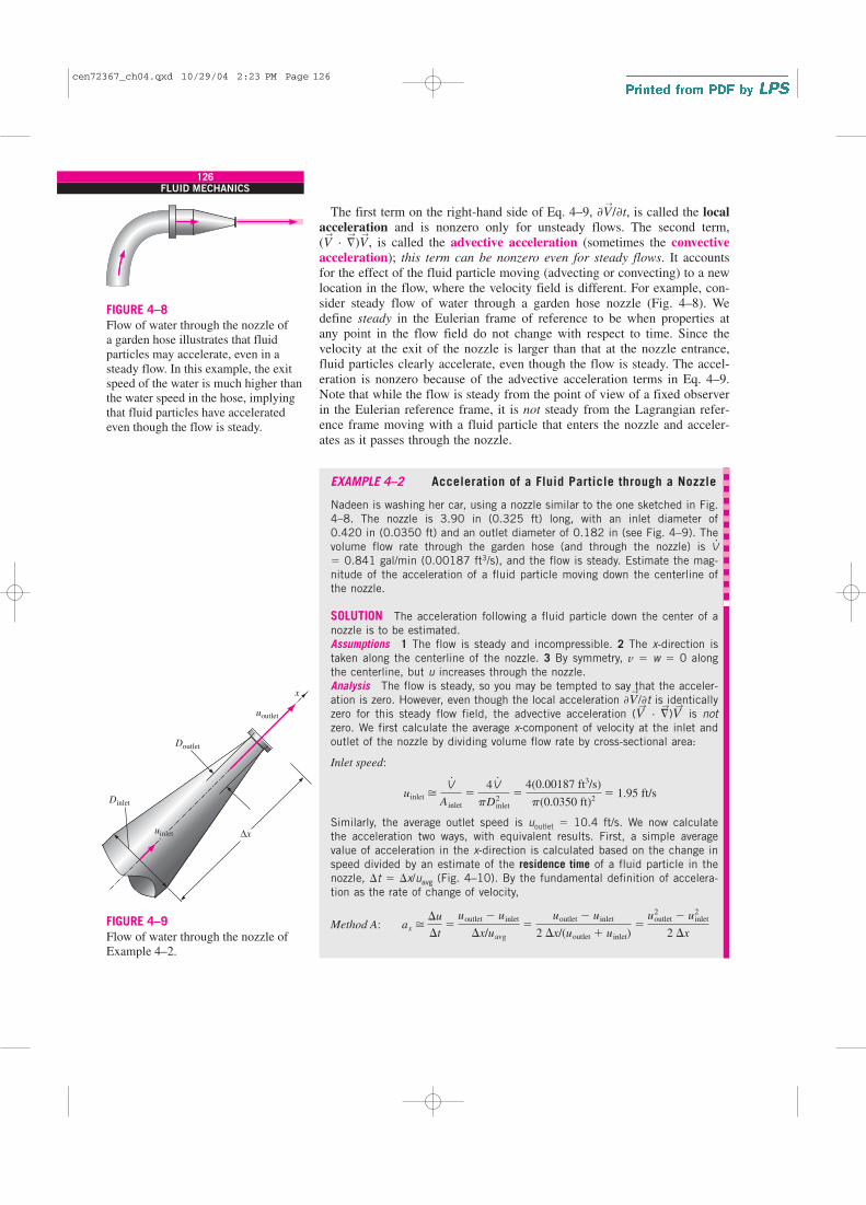
sider steady flow of water through a garden hose nozzle (Fig. 4–8). We

define steady in the Eulerian frame of reference to be when properties at

any point in the flow field do not change with respect to time. Since the

velocity at the exit of the nozzle is larger than that at the nozzle entrance,

fluid particles clearly accelerate, even though the flow is steady. The accel-

eration is nonzero because of the advective acceleration terms in Eq. 4–9.

Note that while the flow is steady from the point of view of a fixed observer

in the Eulerian reference frame, it is not steady from the Lagrangian refer-

ence frame moving with a fluid particle that enters the nozzle and acceler-

ates as it passes through the nozzle.

EXAMPLE 4–2 Acceleration of a Fluid Particle through a Nozzle

Nadeen is washing her car, using a nozzle similar to the one sketched in Fig.

4–8. The nozzle is 3.90 in (0.325 ft) long, with an inlet diameter of

0.420 in (0.0350 ft) and an outlet diameter of 0.182 in (see Fig. 4–9). The

volume flow rate through the garden hose (and through the nozzle) is V.

� 0.841 gal/min (0.00187 ft3/s), and the flow is steady. Estimate the mag-

nitude of the acceleration of a fluid particle moving down the centerline of

the nozzle.

SOLUTION The acceleration following a fluid particle down the center of a

nozzle is to be estimated.

Assumptions 1 The flow is steady and incompressible. 2 The x-direction is

taken along the centerline of the nozzle. 3 By symmetry, v � w � 0 along

the centerline, but u increases through the nozzle.

Analysis The flow is steady, so you may be tempted to say that the acceler-

ation is zero. However, even though the local acceleration �V→

/�t is identically

zero for this steady flow field, the advective acceleration (V→

· �→

)V→

is not

zero. We first calculate the average x-component of velocity at the inlet and

outlet of the nozzle by dividing volume flow rate by cross-sectional area:

Inlet speed:

Similarly, the average outlet speed is uoutlet � 10.4 ft/s. We now calculate

the acceleration two ways, with equivalent results. First, a simple average

value of acceleration in the x-direction is calculated based on the change in

speed divided by an estimate of the residence time of a fluid particle in the

nozzle, �t � �x/uavg (Fig. 4–10). By the fundamental definition of accelera-

tion as the rate of change of velocity,

Method A: ax ��u

�t�

uoutlet � uinlet

�x/uavg

�uoutlet � uinlet

2 �x/(uoutlet � uinlet)�

uoutlet2 � uinlet

2

2 �x

uinlet �V#

Ainlet

�4V#

pD2inlet

�4(0.00187 ft3/s)

p(0.0350 ft)2� 1.95 ft/s

126FLUID MECHANICS

FIGURE 4–8

Flow of water through the nozzle of

a garden hose illustrates that fluid

particles may accelerate, even in a

steady flow. In this example, the exit

speed of the water is much higher than

the water speed in the hose, implying

that fluid particles have accelerated

even though the flow is steady.

Doutlet

Dinlet

uoutlet

x

∆xuinlet

FIGURE 4–9

Flow of water through the nozzle of

Example 4–2.

cen72367_ch04.qxd 10/29/04 2:23 PM Page 126

The second method uses the equation for acceleration field components in

Cartesian coordinates, Eq. 4–11,

Method B:

Steady v � 0 along centerline w � 0 along centerline

Here we see that only one advective term is nonzero. We approximate the

average speed through the nozzle as the average of the inlet and outlet

speeds, and we use a first-order finite difference approximation (Fig. 4–11) for

the average value of derivative �u/�x through the centerline of the nozzle:

The result of method B is identical to that of method A. Substitution of the

given values yields

Axial acceleration:

Discussion Fluid particles are accelerated through the nozzle at nearly five

times the acceleration of gravity (almost five g’s)! This simple example

clearly illustrates that the acceleration of a fluid particle can be nonzero,

even in steady flow. Note that the acceleration is actually a point function,

whereas we have estimated a simple average acceleration through the entire

nozzle.

Material DerivativeThe total derivative operator d/dt in Eq. 4–9 is given a special name, the

material derivative; some authors also assign to it a special notation, D/Dt,

in order to emphasize that it is formed by following a fluid particle as it

moves through the flow field (Fig. 4–12). Other names for the material

derivative include total, particle, Lagrangian, Eulerian, and substantialderivative.

Material derivative: (4–12)

When we apply the material derivative of Eq. 4–12 to the velocity field, the

result is the acceleration field as expressed by Eq. 4–9, which is thus some-

times called the material acceleration.

Material acceleration: (4–13)

Equation 4–12 can also be applied to other fluid properties besides velocity,

both scalars and vectors. For example, the material derivative of pressure

can be written as

Material derivative of pressure: (4–14)DP

Dt�

dP

dt�

�P

�t� (V

→

� §→

)P

a→

(x, y, z, t) �DV

→

Dt�

dV→

dt�

�V→

�t� (V

→

� §→

)V→

D

Dt�

d

dt�

�

�t� (V

→

� §→

)

ax �u2

outlet � u2inlet

2 �x�

(10.4 ft/s)2 � (1.95 ft/s)2

2(0.325 ft)� 160 ft/s2

ax �uoutlet � uinlet

2 uoutlet � uinlet

�x�

uoutlet2 � uinlet

2

2 �x

ax ��u

�t� u

�u

�x� v

�u

�y � w

�u

�z � uavg

�u

�x

127CHAPTER 4

Fluid particle

at time t + ∆t

Fluid particle

at time t

x

∆x

FIGURE 4–10

Residence time �t is defined as the

time it takes for a fluid particle to

travel through the nozzle from inlet

to outlet (distance �x).

q

x

∆x

≅ ∆q

∆x

dq

dx

∆q

FIGURE 4–11

A first-order finite difference

approximation for derivative dq/dx

is simply the change in dependent

variable (q) divided by the change

in independent variable (x).

t

t + dt

t + 2 dt

t + 3 dt

FIGURE 4–12

The material derivative D/Dt is

defined by following a fluid particle

as it moves throughout the flow field.

In this illustration, the fluid particle is

accelerating to the right as it moves

up and to the right.

F 0 0 0— — —

cen72367_ch04.qxd 10/29/04 2:23 PM Page 127

Equation 4–14 represents the time rate of change of pressure following a

fluid particle as it moves through the flow and contains both local

(unsteady) and advective components (Fig. 4–13).

EXAMPLE 4–3 Material Acceleration of a Steady Velocity Field

Consider the steady, incompressible, two-dimensional velocity field of Example

4–1. (a) Calculate the material acceleration at the point (x � 2 m, y � 3 m).

(b) Sketch the material acceleration vectors at the same array of x- and y-

values as in Example 4–1.

SOLUTION For the given velocity field, the material acceleration vector is to

be calculated at a particular point and plotted at an array of locations in the

flow field.

Assumptions 1 The flow is steady and incompressible. 2 The flow is two-

dimensional, implying no z-component of velocity and no variation of u or v

with z.

Analysis (a) Using the velocity field of Eq. 1 of Example 4–1 and the equa-

tion for material acceleration components in Cartesian coordinates (Eq.

4–11), we write expressions for the two nonzero components of the accelera-

tion vector:

and

At the point (x � 2 m, y � 3 m), ax � 1.68 m/s2 and ay � 0.720 m/s2.

(b) The equations in part (a) are applied to an array of x- and y-values in the

flow domain within the given limits, and the acceleration vectors are plotted

in Fig. 4–14.

Discussion The acceleration field is nonzero, even though the flow is

steady. Above the stagnation point (above y � 1.875 m), the acceleration

vectors plotted in Fig. 4–14 point upward, increasing in magnitude away

from the stagnation point. To the right of the stagnation point (to the right of

x � �0.625 m), the acceleration vectors point to the right, again increasing

in magnitude away from the stagnation point. This agrees qualitatively with

the velocity vectors of Fig. 4–4 and the streamlines sketched in Fig. 4–14;

namely, in the upper-right portion of the flow field, fluid particles are accel-

erated in the upper-right direction and therefore veer in the counterclockwise

direction due to centripetal acceleration toward the upper right. The flow

below y � 1.875 m is a mirror image of the flow above this symmetry line,

and flow to the left of x � �0.625 m is a mirror image of the flow to the

right of this symmetry line.

� 0 � (0.5 � 0.8x)(0) � (1.5 � 0.8y)(�0.8) � 0 � (�1.2 � 0.64y) m/s2

ay ��v

�t � u

�v

�x � v

�v

�y � w

�v

�z

� 0 � (0.5 � 0.8x)(0.8) � (15 � 0.8y)(0) � 0 � (0.4 � 0.64x) m/s2

ax ��u

�t � u

�u

�x � v

�u

�y � w

�u

�z

128FLUID MECHANICS

Local

Dt

Materialderivative

V � �

Advective

FIGURE 4–13

The material derivative D/Dt is

composed of a local or unsteady part

and a convective or advective part.

Scale:

5

4

3

2y

1

0

–1

–3 –2 –1 0

x

1 2 3

10 m/s2

FIGURE 4–14

Acceleration vectors for the velocity

field of Examples 4–1 and 4–3. The

scale is shown by the top arrow,

and the solid black curves represent

the approximate shapes of some

streamlines, based on the calculated

velocity vectors (see Fig. 4–4). The

stagnation point is indicated by the

blue circle.

cen72367_ch04.qxd 10/29/04 2:23 PM Page 128

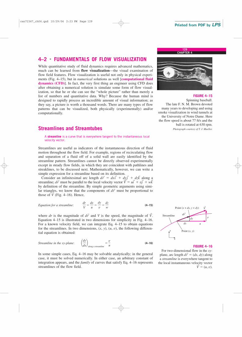
4–2 � FUNDAMENTALS OF FLOW VISUALIZATION

While quantitative study of fluid dynamics requires advanced mathematics,

much can be learned from flow visualization—the visual examination of

flow field features. Flow visualization is useful not only in physical experi-

ments (Fig. 4–15), but in numerical solutions as well [computational fluiddynamics (CFD)]. In fact, the very first thing an engineer using CFD does

after obtaining a numerical solution is simulate some form of flow visual-

ization, so that he or she can see the “whole picture” rather than merely a

list of numbers and quantitative data. Why? Because the human mind is

designed to rapidly process an incredible amount of visual information; as

they say, a picture is worth a thousand words. There are many types of flow

patterns that can be visualized, both physically (experimentally) and/or

computationally.

Streamlines and Streamtubes

A streamline is a curve that is everywhere tangent to the instantaneous localvelocity vector.

Streamlines are useful as indicators of the instantaneous direction of fluid

motion throughout the flow field. For example, regions of recirculating flow

and separation of a fluid off of a solid wall are easily identified by the

streamline pattern. Streamlines cannot be directly observed experimentally

except in steady flow fields, in which they are coincident with pathlines and

streaklines, to be discussed next. Mathematically, however, we can write a

simple expression for a streamline based on its definition.

Consider an infinitesimal arc length dr→

� dxi→

� dyj→

� dzk→

along a

streamline; dr→

must be parallel to the local velocity vector V→

� ui→

� vj→

� wk→

by definition of the streamline. By simple geometric arguments using simi-

lar triangles, we know that the components of dr→

must be proportional to

those of V→

(Fig. 4–16). Hence,

Equation for a streamline: (4–15)

where dr is the magnitude of dr→

and V is the speed, the magnitude of V→

.

Equation 4–15 is illustrated in two dimensions for simplicity in Fig. 4–16.

For a known velocity field, we can integrate Eq. 4–15 to obtain equations

for the streamlines. In two dimensions, (x, y), (u, v), the following differen-

tial equation is obtained:

Streamline in the xy-plane: (4–16)

In some simple cases, Eq. 4–16 may be solvable analytically; in the general

case, it must be solved numerically. In either case, an arbitrary constant of

integration appears, and the family of curves that satisfy Eq. 4–16 represents

streamlines of the flow field.

ady

dxb

along a streamline

�v

u

dr

V�

dx

u�

dy

v

�dz

w

129CHAPTER 4

FIGURE 4–15

Spinning baseball.

The late F. N. M. Brown devoted

many years to developing and using

smoke visualization in wind tunnels at

the University of Notre Dame. Here

the flow speed is about 77 ft/s and the

ball is rotated at 630 rpm.

Photograph courtesy of T. J. Mueller.

y

x

Point (x, y)

Streamline

Point (x + dx, y + dy)

dx

dy

u

v

V

dr→

→

FIGURE 4–16

For two-dimensional flow in the xy-

plane, arc length dr→

� (dx, dy) along

a streamline is everywhere tangent to

the local instantaneous velocity vector

V→

� (u, v).

cen72367_ch04.qxd 10/29/04 2:23 PM Page 129

EXAMPLE 4–4 Streamlines in the xy-Plane—An Analytical

Solution

For the steady, incompressible, two-dimensional velocity field of Example

4–1, plot several streamlines in the right half of the flow (x � 0) and com-

pare to the velocity vectors plotted in Fig. 4–4.

SOLUTION An analytical expression for streamlines is to be generated and

plotted in the upper-right quadrant.

Assumptions 1 The flow is steady and incompressible. 2 The flow is two-

dimensional, implying no z-component of velocity and no variation of u or v

with z.

Analysis Equation 4–16 is applicable here; thus, along a streamline,

We solve this differential equation by separation of variables:

After some algebra (which we leave to the reader), we solve for y as a func-

tion of x along a streamline,

where C is a constant of integration that can be set to various values in order

to plot the streamlines. Several streamlines of the given flow field are shown

in Fig. 4–17.

Discussion The velocity vectors of Fig. 4–4 are superimposed on the

streamlines of Fig. 4–17; the agreement is excellent in the sense that the

velocity vectors point everywhere tangent to the streamlines. Note that speed

cannot be determined directly from the streamlines alone.

A streamtube consists of a bundle of streamlines (Fig. 4–18), much like

a communications cable consists of a bundle of fiber-optic cables. Since

streamlines are everywhere parallel to the local velocity, fluid cannot cross a

streamline by definition. By extension, fluid within a streamtube must

remain there and cannot cross the boundary of the streamtube. You must

keep in mind that both streamlines and streamtubes are instantaneous quan-

tities, defined at a particular instant in time according to the velocity field at

that instant. In an unsteady flow, the streamline pattern may change signifi-

cantly with time. Nevertheless, at any instant in time, the mass flow rate

passing through any cross-sectional slice of a given streamtube must remain

the same. For example, in a converging portion of an incompressible flow

field, the diameter of the streamtube must decrease as the velocity increases

so as to conserve mass (Fig. 4–19a). Likewise, the streamtube diameter

increases in diverging portions of the incompressible flow (Fig. 4–19b).

Pathlines

A pathline is the actual path traveled by an individual fluid particle over sometime period.

y �C

0.8(0.5 � 0.8x)� 1.875

dy

1.5 � 0.8y�

dx

0.5 � 0.8x → � dy

1.5 � 0.8y� � dx

0.5 � 0.8x

dy

dx�

1.5 � 0.8y

0.5 � 0.8x

130FLUID MECHANICS

5

4

3

2y

1

0

–1

0 1 2 3

x

4 5

FIGURE 4–17

Streamlines (solid black curves) for

the velocity field of Example 4–4;

velocity vectors of Fig. 4–4 (blue

arrows) are superimposed for

comparison.

Streamlines

Streamtube

FIGURE 4–18

A streamtube consists of a bundle of

individual streamlines.

cen72367_ch04.qxd 10/29/04 2:23 PM Page 130

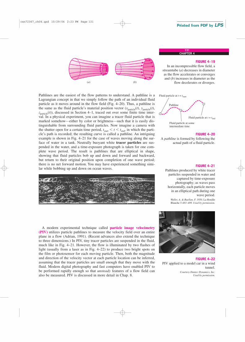
Pathlines are the easiest of the flow patterns to understand. A pathline is a

Lagrangian concept in that we simply follow the path of an individual fluid

particle as it moves around in the flow field (Fig. 4–20). Thus, a pathline is

the same as the fluid particle’s material position vector (xparticle(t), yparticle(t),

zparticle(t)), discussed in Section 4–1, traced out over some finite time inter-

val. In a physical experiment, you can imagine a tracer fluid particle that is

marked somehow—either by color or brightness—such that it is easily dis-

tinguishable from surrounding fluid particles. Now imagine a camera with

the shutter open for a certain time period, tstart t tend, in which the parti-

cle’s path is recorded; the resulting curve is called a pathline. An intriguing

example is shown in Fig. 4–21 for the case of waves moving along the sur-

face of water in a tank. Neutrally buoyant white tracer particles are sus-

pended in the water, and a time-exposure photograph is taken for one com-

plete wave period. The result is pathlines that are elliptical in shape,

showing that fluid particles bob up and down and forward and backward,

but return to their original position upon completion of one wave period;

there is no net forward motion. You may have experienced something simi-

lar while bobbing up and down on ocean waves.

131CHAPTER 4

(b)(a)

FIGURE 4–19

In an incompressible flow field, a

streamtube (a) decreases in diameter

as the flow accelerates or converges

and (b) increases in diameter as the

flow decelerates or diverges.

A modern experimental technique called particle image velocimetry(PIV) utilizes particle pathlines to measure the velocity field over an entire

plane in a flow (Adrian, 1991). (Recent advances also extend the technique

to three dimensions.) In PIV, tiny tracer particles are suspended in the fluid,

much like in Fig. 4–21. However, the flow is illuminated by two flashes of

light (usually from a laser as in Fig. 4–22) to produce two bright spots on

the film or photosensor for each moving particle. Then, both the magnitude

and direction of the velocity vector at each particle location can be inferred,

assuming that the tracer particles are small enough that they move with the

fluid. Modern digital photography and fast computers have enabled PIV to

be performed rapidly enough so that unsteady features of a flow field can

also be measured. PIV is discussed in more detail in Chap. 8.

Fluid particle at t = tstart

Fluid particle at t = tend

Fluid particle at someintermediate time

Pathline

FIGURE 4–20

A pathline is formed by following the

actual path of a fluid particle.

FIGURE 4–22

PIV applied to a model car in a wind

tunnel.

Courtesy Dantec Dynamics, Inc.

Used by permission.

FIGURE 4–21

Pathlines produced by white tracer

particles suspended in water and

captured by time-exposure

photography; as waves pass

horizontally, each particle moves

in an elliptical path during one

wave period.

Wallet, A. & Ruellan, F. 1950, La Houille

Blanche 5:483–489. Used by permission.

cen72367_ch04.qxd 10/29/04 2:23 PM Page 131

Pathlines can also be calculated numerically for a known velocity field.

Specifically, the location of the tracer particle is integrated over time from

some starting location x→

start and starting time tstart to some later time t.

Tracer particle location at time t: (4–17)

When Eq. 4–17 is calculated for t between tstart and tend, a plot of x→

(t) is the

pathline of the fluid particle during that time interval, as illustrated in Fig.

4–20. For some simple flow fields, Eq. 4–17 can be integrated analytically.

For more complex flows, we must perform a numerical integration.

If the velocity field is steady, individual fluid particles will follow stream-

lines. Thus, for steady flow, pathlines are identical to streamlines.

Streaklines

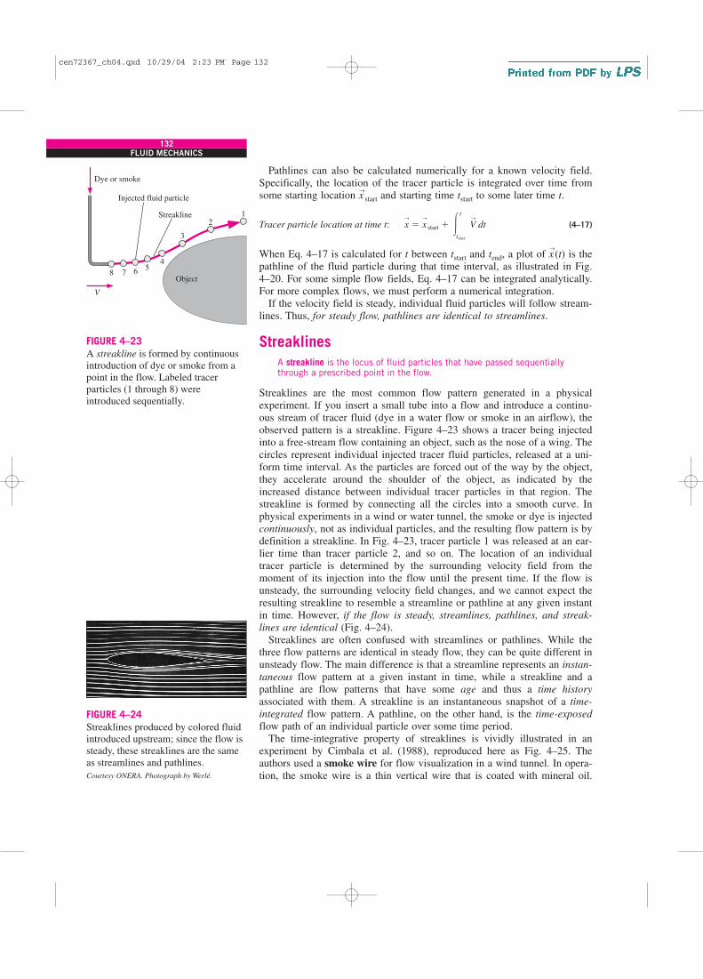
A streakline is the locus of fluid particles that have passed sequentiallythrough a prescribed point in the flow.

Streaklines are the most common flow pattern generated in a physical

experiment. If you insert a small tube into a flow and introduce a continu-

ous stream of tracer fluid (dye in a water flow or smoke in an airflow), the

observed pattern is a streakline. Figure 4–23 shows a tracer being injected

into a free-stream flow containing an object, such as the nose of a wing. The

circles represent individual injected tracer fluid particles, released at a uni-

form time interval. As the particles are forced out of the way by the object,

they accelerate around the shoulder of the object, as indicated by the

increased distance between individual tracer particles in that region. The

streakline is formed by connecting all the circles into a smooth curve. In

physical experiments in a wind or water tunnel, the smoke or dye is injected

continuously, not as individual particles, and the resulting flow pattern is by

definition a streakline. In Fig. 4–23, tracer particle 1 was released at an ear-

lier time than tracer particle 2, and so on. The location of an individual

tracer particle is determined by the surrounding velocity field from the

moment of its injection into the flow until the present time. If the flow is

unsteady, the surrounding velocity field changes, and we cannot expect the

resulting streakline to resemble a streamline or pathline at any given instant

in time. However, if the flow is steady, streamlines, pathlines, and streak-

lines are identical (Fig. 4–24).

Streaklines are often confused with streamlines or pathlines. While the

three flow patterns are identical in steady flow, they can be quite different in

unsteady flow. The main difference is that a streamline represents an instan-

taneous flow pattern at a given instant in time, while a streakline and a

pathline are flow patterns that have some age and thus a time history

associated with them. A streakline is an instantaneous snapshot of a time-

integrated flow pattern. A pathline, on the other hand, is the time-exposed

flow path of an individual particle over some time period.

The time-integrative property of streaklines is vividly illustrated in an

experiment by Cimbala et al. (1988), reproduced here as Fig. 4–25. The

authors used a smoke wire for flow visualization in a wind tunnel. In opera-

tion, the smoke wire is a thin vertical wire that is coated with mineral oil.

x→

� x→

start � �t

tstart

V→

dt

132FLUID MECHANICS

V

Streakline

Object8 7 6

54

3

21

Injected fluid particle

Dye or smoke

FIGURE 4–23

A streakline is formed by continuous

introduction of dye or smoke from a

point in the flow. Labeled tracer

particles (1 through 8) were

introduced sequentially.

FIGURE 4–24

Streaklines produced by colored fluid

introduced upstream; since the flow is

steady, these streaklines are the same

as streamlines and pathlines.

Courtesy ONERA. Photograph by Werlé.

cen72367_ch04.qxd 10/29/04 2:23 PM Page 132

The oil breaks up into beads along the length of the wire due to surface ten-

sion effects. When an electric current heats the wire, each little bead of oil

produces a streakline of smoke. In Fig. 4–25a, streaklines are introduced

from a smoke wire located just downstream of a circular cylinder of diameter

D aligned normal to the plane of view. (When multiple streaklines are intro-

duced along a line, as in Fig. 4–25, we refer to this as a rake of streaklines.)

The Reynolds number of the flow is Re � rVD/m � 93. Because of unsteady

vortices shed in an alternating pattern from the cylinder, the smoke collects

into a clearly defined pattern called a Kármán vortex street.From Fig. 4–25a alone, one may think that the shed vortices continue to

exist to several hundred diameters downstream of the cylinder. However, the

streakline pattern of this figure is misleading! In Fig. 4–25b, the smoke wire

is placed 150 diameters downstream of the cylinder. The resulting streaklines

are straight, indicating that the shed vortices have in reality disappeared by

this downstream distance. The flow is steady and parallel at this location, and

there are no more vortices; viscous diffusion has caused adjacent vortices of

opposite sign to cancel each other out by around 100 cylinder diameters. The

patterns of Fig. 4–25a near x/D � 150 are merely remnants of the vortex

street that existed upstream. The streaklines of Fig. 4–25b, however, show

the correct features of the flow at that location. The streaklines generated at

x/D � 150 are identical to streamlines or pathlines in that region of the

flow—straight, nearly horizontal lines—since the flow is steady there.

For a known velocity field, a streakline can be generated numerically,

although with some difficulty. One needs to follow the paths of a continuous

stream of tracer particles from the time of their injection into the flow until

the present time, using Eq. 4–17. Mathematically, the location of a tracer

particle is integrated over time from the time of its injection tinject to the

present time tpresent. Equation 4–17 becomes

Integrated tracer particle location: (4–18)x→

� x→

injection � �tpresent

tinject

V→

dt

133CHAPTER 4

(a)

(b)

0 50

Cylinder

x/D

100 150 200 250

Cylinder

FIGURE 4–25

Smoke streaklines introduced by a smoke wire at two different locations in the

wake of a circular cylinder: (a) smoke wire just downstream of the cylinder and

(b) smoke wire located at x/D = 150. The time-integrative nature of streaklines

is clearly seen by comparing the two photographs.

Photos by John M. Cimbala.

cen72367_ch04.qxd 10/29/04 2:23 PM Page 133

134FLUID MECHANICS

5

4

3

2y

1

0

–1

0

x

1 2

Streamlines at t = 2 s

3 4 5

Pathlines for 0 < t < 2 s

Streaklines for 0 < t < 2 s

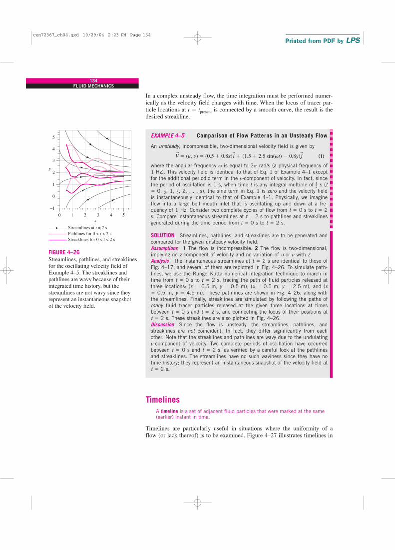
FIGURE 4–26

Streamlines, pathlines, and streaklines

for the oscillating velocity field of

Example 4–5. The streaklines and

pathlines are wavy because of their

integrated time history, but the

streamlines are not wavy since they

represent an instantaneous snapshot

of the velocity field.

In a complex unsteady flow, the time integration must be performed numer-

ically as the velocity field changes with time. When the locus of tracer par-

ticle locations at t � tpresent is connected by a smooth curve, the result is the

desired streakline.

EXAMPLE 4–5 Comparison of Flow Patterns in an Unsteady Flow

An unsteady, incompressible, two-dimensional velocity field is given by

(1)

where the angular frequency v is equal to 2p rad/s (a physical frequency of

1 Hz). This velocity field is identical to that of Eq. 1 of Example 4–1 except

for the additional periodic term in the v-component of velocity. In fact, since

the period of oscillation is 1 s, when time t is any integral multiple of s (t

� 0, , 1, , 2, . . . s), the sine term in Eq. 1 is zero and the velocity field

is instantaneously identical to that of Example 4–1. Physically, we imagine

flow into a large bell mouth inlet that is oscillating up and down at a fre-

quency of 1 Hz. Consider two complete cycles of flow from t � 0 s to t � 2

s. Compare instantaneous streamlines at t � 2 s to pathlines and streaklines

generated during the time period from t � 0 s to t � 2 s.

SOLUTION Streamlines, pathlines, and streaklines are to be generated and

compared for the given unsteady velocity field.

Assumptions 1 The flow is incompressible. 2 The flow is two-dimensional,

implying no z-component of velocity and no variation of u or v with z.

Analysis The instantaneous streamlines at t � 2 s are identical to those of

Fig. 4–17, and several of them are replotted in Fig. 4–26. To simulate path-

lines, we use the Runge–Kutta numerical integration technique to march in

time from t � 0 s to t � 2 s, tracing the path of fluid particles released at

three locations: (x � 0.5 m, y � 0.5 m), (x � 0.5 m, y � 2.5 m), and (x

� 0.5 m, y � 4.5 m). These pathlines are shown in Fig. 4–26, along with

the streamlines. Finally, streaklines are simulated by following the paths of

many fluid tracer particles released at the given three locations at times

between t � 0 s and t � 2 s, and connecting the locus of their positions at

t � 2 s. These streaklines are also plotted in Fig. 4–26.

Discussion Since the flow is unsteady, the streamlines, pathlines, and

streaklines are not coincident. In fact, they differ significantly from each

other. Note that the streaklines and pathlines are wavy due to the undulating

v-component of velocity. Two complete periods of oscillation have occurred

between t � 0 s and t � 2 s, as verified by a careful look at the pathlines

and streaklines. The streamlines have no such waviness since they have no

time history; they represent an instantaneous snapshot of the velocity field at

t � 2 s.

Timelines

A timeline is a set of adjacent fluid particles that were marked at the same(earlier) instant in time.

Timelines are particularly useful in situations where the uniformity of a

flow (or lack thereof) is to be examined. Figure 4–27 illustrates timelines in

32

12

12

V→

� (u, v) � (0.5 � 0.8x) i→

� (1.5 � 2.5 sin(vt) � 0.8y) j→

cen72367_ch04.qxd 10/29/04 2:23 PM Page 134

a channel flow between two parallel walls. Because of friction at the walls,

the fluid velocity there is zero (the no-slip condition), and the top and bot-

tom of the timeline are anchored at their starting locations. In regions of the

flow away from the walls, the marked fluid particles move at the local fluid

velocity, deforming the timeline. In the example of Fig. 4–27, the speed

near the center of the channel is fairly uniform, but small deviations tend to

amplify with time as the timeline stretches. Timelines can be generated

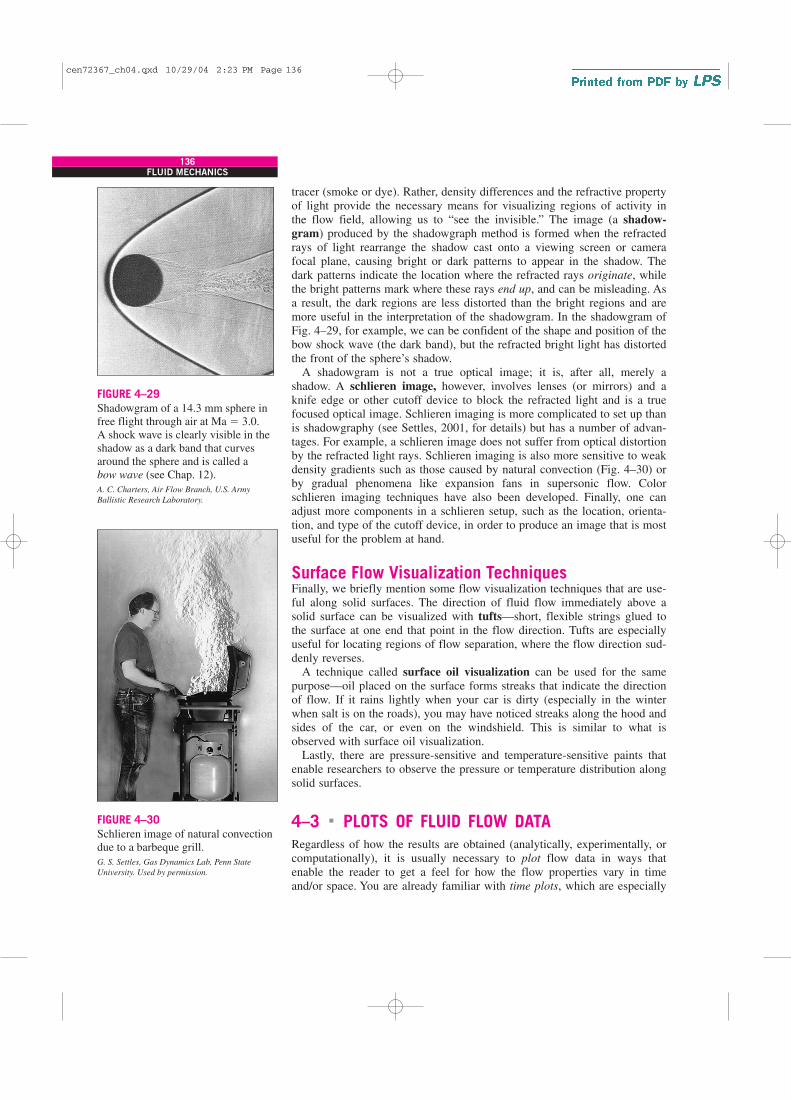
experimentally in a water channel through use of a hydrogen bubble wire.When a short burst of electric current is sent through the cathode wire, elec-

trolysis of the water occurs and tiny hydrogen gas bubbles form at the wire.

Since the bubbles are so small, their buoyancy is nearly negligible, and the

bubbles follow the water flow nicely (Fig. 4–28).

Refractive Flow Visualization TechniquesAnother category of flow visualization is based on the refractive propertyof light waves. As you recall from your study of physics, the speed of light

through one material may differ somewhat from that in another material, or

even in the same material if its density changes. As light travels through one

fluid into a fluid with a different index of refraction, the light rays bend

(they are refracted).

There are two primary flow visualization techniques that utilize the fact

that the index of refraction in air (or other gases) varies with density. They

are the shadowgraph technique and the schlieren technique (Settles,

2001). Interferometry is a visualization technique that utilizes the related

phase change of light as it passes through air of varying densities as the

basis for flow visualization and is not discussed here (see Merzkirch, 1987).

All these techniques are useful for flow visualization in flow fields where

density changes from one location in the flow to another, such as natural

convection flows (temperature differences cause the density variations),

mixing flows (fluid species cause the density variations), and supersonic

flows (shock waves and expansion waves cause the density variations).

Unlike flow visualizations involving streaklines, pathlines, and timelines,

the shadowgraph and schlieren methods do not require injection of a visible

135CHAPTER 4

Timeline at t = 0

Timeline at t = t1

Timeline at t = t2

Timeline at t = t3

Flow

FIGURE 4–27

Timelines are formed by marking a

line of fluid particles, and then

watching that line move (and deform)

through the flow field; timelines are

shown at t � 0, t1, t2, and t3.

FIGURE 4–28

Timelines produced by a hydrogen

bubble wire are used to visualize the

boundary layer velocity profile shape.

Flow is from left to right, and the

hydrogen bubble wire is located to the

left of the field of view. Bubbles near

the wall reveal a flow instability that

leads to turbulence.

Bippes, H. 1972 Sitzungsber, Heidelb. Akad. Wiss.

Math. Naturwiss. Kl., no. 3, 103–180; NASA TM-

75243, 1978.

cen72367_ch04.qxd 10/29/04 2:23 PM Page 135

tracer (smoke or dye). Rather, density differences and the refractive property

of light provide the necessary means for visualizing regions of activity in

the flow field, allowing us to “see the invisible.” The image (a shadow-gram) produced by the shadowgraph method is formed when the refracted

rays of light rearrange the shadow cast onto a viewing screen or camera

focal plane, causing bright or dark patterns to appear in the shadow. The

dark patterns indicate the location where the refracted rays originate, while

the bright patterns mark where these rays end up, and can be misleading. As

a result, the dark regions are less distorted than the bright regions and are

more useful in the interpretation of the shadowgram. In the shadowgram of

Fig. 4–29, for example, we can be confident of the shape and position of the

bow shock wave (the dark band), but the refracted bright light has distorted

the front of the sphere’s shadow.

A shadowgram is not a true optical image; it is, after all, merely a

shadow. A schlieren image, however, involves lenses (or mirrors) and a

knife edge or other cutoff device to block the refracted light and is a true

focused optical image. Schlieren imaging is more complicated to set up than

is shadowgraphy (see Settles, 2001, for details) but has a number of advan-

tages. For example, a schlieren image does not suffer from optical distortion

by the refracted light rays. Schlieren imaging is also more sensitive to weak

density gradients such as those caused by natural convection (Fig. 4–30) or

by gradual phenomena like expansion fans in supersonic flow. Color

schlieren imaging techniques have also been developed. Finally, one can

adjust more components in a schlieren setup, such as the location, orienta-

tion, and type of the cutoff device, in order to produce an image that is most

useful for the problem at hand.

Surface Flow Visualization TechniquesFinally, we briefly mention some flow visualization techniques that are use-

ful along solid surfaces. The direction of fluid flow immediately above a

solid surface can be visualized with tufts—short, flexible strings glued to

the surface at one end that point in the flow direction. Tufts are especially

useful for locating regions of flow separation, where the flow direction sud-

denly reverses.

A technique called surface oil visualization can be used for the same

purpose—oil placed on the surface forms streaks that indicate the direction

of flow. If it rains lightly when your car is dirty (especially in the winter

when salt is on the roads), you may have noticed streaks along the hood and

sides of the car, or even on the windshield. This is similar to what is

observed with surface oil visualization.

Lastly, there are pressure-sensitive and temperature-sensitive paints that

enable researchers to observe the pressure or temperature distribution along

solid surfaces.

4–3 � PLOTS OF FLUID FLOW DATA

Regardless of how the results are obtained (analytically, experimentally, or

computationally), it is usually necessary to plot flow data in ways that

enable the reader to get a feel for how the flow properties vary in time

and/or space. You are already familiar with time plots, which are especially

136FLUID MECHANICS

FIGURE 4–29

Shadowgram of a 14.3 mm sphere in

free flight through air at Ma � 3.0.

A shock wave is clearly visible in the

shadow as a dark band that curves

around the sphere and is called a

bow wave (see Chap. 12).

A. C. Charters, Air Flow Branch, U.S. Army

Ballistic Research Laboratory.

FIGURE 4–30

Schlieren image of natural convection

due to a barbeque grill.

G. S. Settles, Gas Dynamics Lab, Penn State

University. Used by permission.

cen72367_ch04.qxd 10/29/04 2:23 PM Page 136

useful in turbulent flows (e.g., a velocity component plotted as a function of

time), and xy-plots (e.g., pressure as a function of radius). In this section,

we discuss three additional types of plots that are useful in fluid mechan-

ics—profile plots, vector plots, and contour plots.

Profile Plots

A profile plot indicates how the value of a scalar property varies along somedesired direction in the flow field.

Profile plots are the simplest of the three to understand because they are like

the common xy-plots that you have generated since grade school. Namely,

you plot how one variable y varies as a function of a second variable x. In

fluid mechanics, profile plots of any scalar variable (pressure, temperature,

density, etc.) can be created, but the most common one used in this book is

the velocity profile plot. We note that since velocity is a vector quantity, we

usually plot either the magnitude of velocity or one of the components of

the velocity vector as a function of distance in some desired direction.

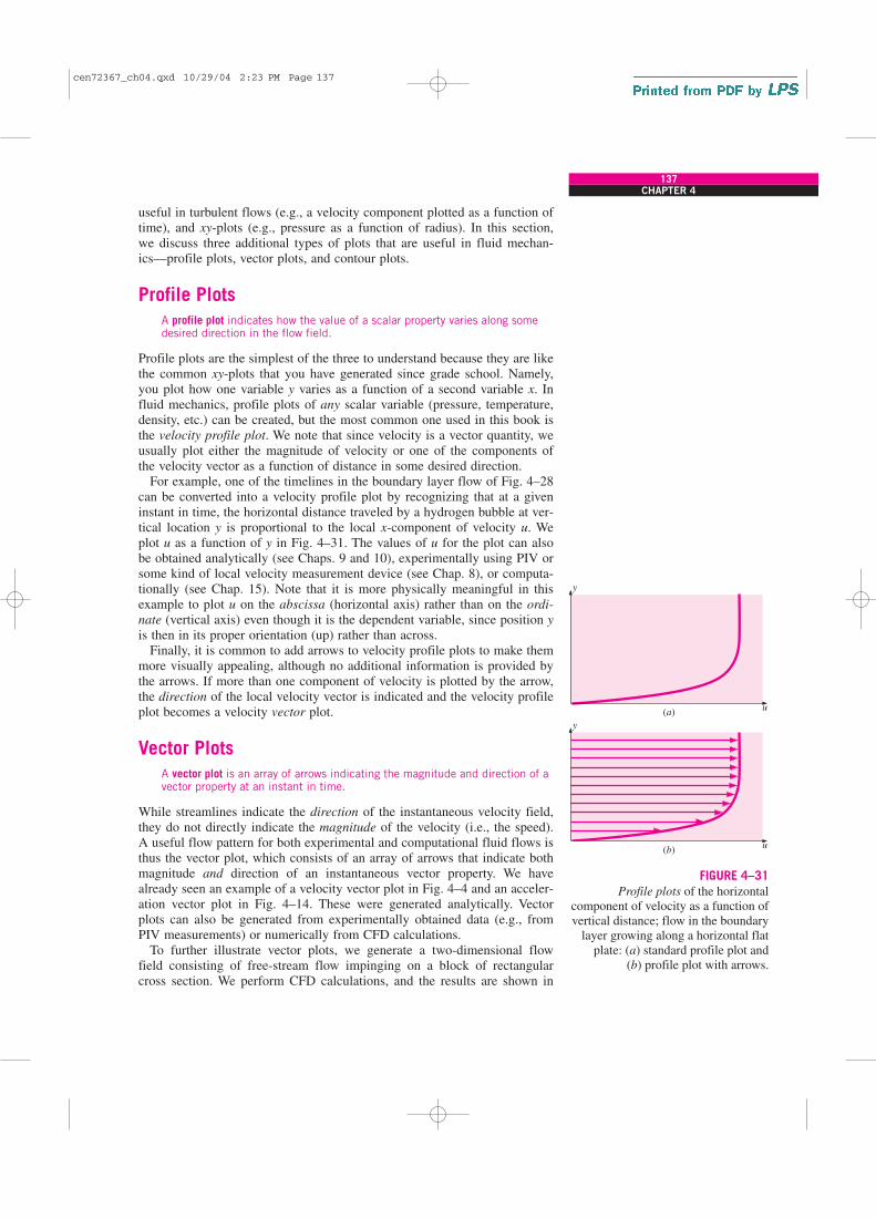
For example, one of the timelines in the boundary layer flow of Fig. 4–28

can be converted into a velocity profile plot by recognizing that at a given

instant in time, the horizontal distance traveled by a hydrogen bubble at ver-

tical location y is proportional to the local x-component of velocity u. We

plot u as a function of y in Fig. 4–31. The values of u for the plot can also

be obtained analytically (see Chaps. 9 and 10), experimentally using PIV or

some kind of local velocity measurement device (see Chap. 8), or computa-

tionally (see Chap. 15). Note that it is more physically meaningful in this

example to plot u on the abscissa (horizontal axis) rather than on the ordi-

nate (vertical axis) even though it is the dependent variable, since position y

is then in its proper orientation (up) rather than across.

Finally, it is common to add arrows to velocity profile plots to make them

more visually appealing, although no additional information is provided by

the arrows. If more than one component of velocity is plotted by the arrow,

the direction of the local velocity vector is indicated and the velocity profile

plot becomes a velocity vector plot.

Vector Plots

A vector plot is an array of arrows indicating the magnitude and direction of avector property at an instant in time.

While streamlines indicate the direction of the instantaneous velocity field,

they do not directly indicate the magnitude of the velocity (i.e., the speed).

A useful flow pattern for both experimental and computational fluid flows is

thus the vector plot, which consists of an array of arrows that indicate both

magnitude and direction of an instantaneous vector property. We have

already seen an example of a velocity vector plot in Fig. 4–4 and an acceler-

ation vector plot in Fig. 4–14. These were generated analytically. Vector

plots can also be generated from experimentally obtained data (e.g., from

PIV measurements) or numerically from CFD calculations.

To further illustrate vector plots, we generate a two-dimensional flow

field consisting of free-stream flow impinging on a block of rectangular

cross section. We perform CFD calculations, and the results are shown in

137CHAPTER 4

y

(a)u

y

(b)u

FIGURE 4–31

Profile plots of the horizontal

component of velocity as a function of

vertical distance; flow in the boundary

layer growing along a horizontal flat

plate: (a) standard profile plot and

(b) profile plot with arrows.

cen72367_ch04.qxd 10/29/04 2:23 PM Page 137

Fig. 4–32. Note that this flow is by nature turbulent and unsteady, but only

the long-time averaged results are calculated and displayed here. Stream-

lines are plotted in Fig. 4–32a; a view of the entire block and a large portion

of its wake is shown. The closed streamlines above and below the symmetry

plane indicate large recirculating eddies, one above and one below the line

of symmetry. A velocity vector plot is shown in Fig. 4–32b. (Only the upper

half of the flow is shown because of symmetry.) It is clear from this plot

that the flow accelerates around the upstream corner of the block, so much

so in fact that the boundary layer cannot negotiate the sharp corner and sep-

arates off the block, producing the large recirculating eddies downstream of

the block. (Note that these velocity vectors are time-averaged values; the

instantaneous vectors change in both magnitude and direction with time as

vortices are shed from the body, similar to those of Fig. 4–25a.) A close-up

view of the separated flow region is plotted in Fig. 4–32c, where we verify

the reverse flow in the lower half of the large recirculating eddy.

Modern CFD codes and postprocessors can add color to a vector plot. For

example, the vectors can be colored according to some other flow property

such as pressure (red for high pressure and blue for low pressure) or tem-

perature (red for hot and blue for cold). In this manner, one can easily visu-

alize not only the magnitude and direction of the flow, but other properties

as well, simultaneously.

Contour Plots

A contour plot shows curves of constant values of a scalar property (ormagnitude of a vector property) at an instant in time.

If you do any hiking, you are familiar with contour maps of mountain trails.

The maps consist of a series of closed curves, each indicating a constant

elevation or altitude. Near the center of a group of such curves is the

mountain peak or valley; the actual peak or valley is a point on the map

showing the highest or lowest elevation. Such maps are useful in that not

only do you get a bird’s-eye view of the streams and trails, etc., but you can

also easily see your elevation and where the trail is flat or steep. In fluid

mechanics, the same principle is applied to various scalar flow properties;

contour plots (also called isocontour plots) are generated of pressure, tem-

perature, velocity magnitude, species concentration, properties of turbu-

lence, etc. A contour plot can quickly reveal regions of high (or low) values

of the flow property being studied.

A contour plot may consist simply of curves indicating various levels of

the property; this is called a contour line plot. Alternatively, the contours

can be filled in with either colors or shades of gray; this is called a filledcontour plot. An example of pressure contours is shown in Fig. 4–33 for

the same flow as in Fig. 4–32. In Fig. 4–33a, filled contours are shown

using shades of gray to identify regions of different pressure levels—dark

regions indicate low pressure and light regions indicate high pressure. It is

clear from this figure that the pressure is highest at the front face of the

block and lowest along the top of the block in the separated zone. The pres-

sure is also low in the wake of the block, as expected. In Fig. 4–33b, the

same pressure contours are shown, but as a contour line plot with labeled

levels of gage pressure in units of pascals.

138FLUID MECHANICS

Recirculating eddy

Symmetry plane

(a)

(b)

(c)

Symmetry plane

Block

Block

FLOW

Block

FLOW

FIGURE 4–32

Results of CFD calculations of flow

impinging on a block; (a) streamlines,

(b) velocity vector plot of the upper

half of the flow, and (c) velocity vector

plot, close-up view revealing more

details.

cen72367_ch04.qxd 10/29/04 2:23 PM Page 138

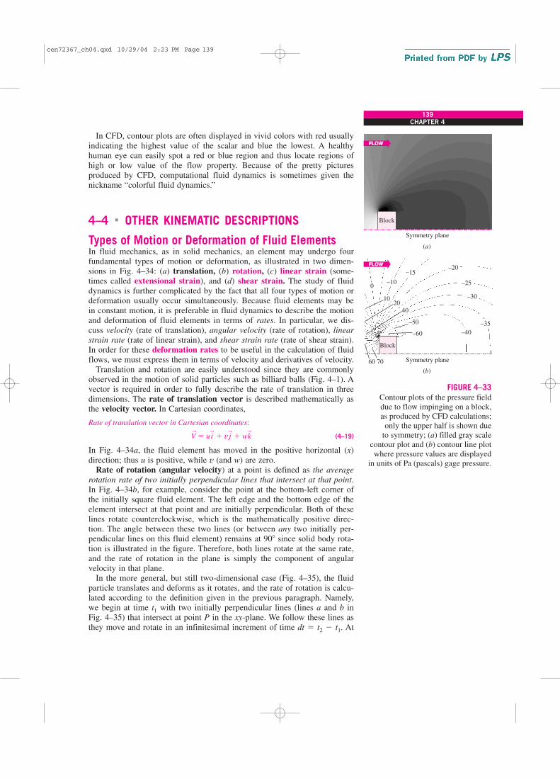
In CFD, contour plots are often displayed in vivid colors with red usually

indicating the highest value of the scalar and blue the lowest. A healthy

human eye can easily spot a red or blue region and thus locate regions of

high or low value of the flow property. Because of the pretty pictures

produced by CFD, computational fluid dynamics is sometimes given the

nickname “colorful fluid dynamics.”

4–4 � OTHER KINEMATIC DESCRIPTIONS

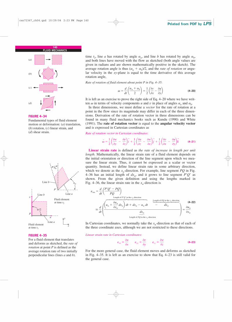
Types of Motion or Deformation of Fluid ElementsIn fluid mechanics, as in solid mechanics, an element may undergo four

fundamental types of motion or deformation, as illustrated in two dimen-

sions in Fig. 4–34: (a) translation, (b) rotation, (c) linear strain (some-

times called extensional strain), and (d) shear strain. The study of fluid

dynamics is further complicated by the fact that all four types of motion or

deformation usually occur simultaneously. Because fluid elements may be

in constant motion, it is preferable in fluid dynamics to describe the motion

and deformation of fluid elements in terms of rates. In particular, we dis-

cuss velocity (rate of translation), angular velocity (rate of rotation), linear

strain rate (rate of linear strain), and shear strain rate (rate of shear strain).

In order for these deformation rates to be useful in the calculation of fluid

flows, we must express them in terms of velocity and derivatives of velocity.

Translation and rotation are easily understood since they are commonly

observed in the motion of solid particles such as billiard balls (Fig. 4–1). A

vector is required in order to fully describe the rate of translation in three

dimensions. The rate of translation vector is described mathematically as

the velocity vector. In Cartesian coordinates,

Rate of translation vector in Cartesian coordinates:

(4–19)

In Fig. 4–34a, the fluid element has moved in the positive horizontal (x)

direction; thus u is positive, while v (and w) are zero.

Rate of rotation (angular velocity) at a point is defined as the average

rotation rate of two initially perpendicular lines that intersect at that point.

In Fig. 4–34b, for example, consider the point at the bottom-left corner of

the initially square fluid element. The left edge and the bottom edge of the

element intersect at that point and are initially perpendicular. Both of these

lines rotate counterclockwise, which is the mathematically positive direc-

tion. The angle between these two lines (or between any two initially per-

pendicular lines on this fluid element) remains at 90 since solid body rota-

tion is illustrated in the figure. Therefore, both lines rotate at the same rate,

and the rate of rotation in the plane is simply the component of angular

velocity in that plane.

In the more general, but still two-dimensional case (Fig. 4–35), the fluid

particle translates and deforms as it rotates, and the rate of rotation is calcu-

lated according to the definition given in the previous paragraph. Namely,

we begin at time t1 with two initially perpendicular lines (lines a and b in

Fig. 4–35) that intersect at point P in the xy-plane. We follow these lines as

they move and rotate in an infinitesimal increment of time dt � t2 � t1. At

V→

� ui→

� v j→

� wk→

139CHAPTER 4

Block

Block

Symmetry plane

Symmetry plane

FLOW

FLOW

(a)

(b)

0–10

–15–20

–25

–30

–35

–40–60

60 70

–50

1020

40

FIGURE 4–33

Contour plots of the pressure field

due to flow impinging on a block,

as produced by CFD calculations;

only the upper half is shown due

to symmetry; (a) filled gray scale

contour plot and (b) contour line plot

where pressure values are displayed

in units of Pa (pascals) gage pressure.

cen72367_ch04.qxd 10/29/04 2:23 PM Page 139

time t2, line a has rotated by angle aa, and line b has rotated by angle ab,

and both lines have moved with the flow as sketched (both angle values are

given in radians and are shown mathematically positive in the sketch). The

average rotation angle is thus (aa � ab)/2, and the rate of rotation or angu-

lar velocity in the xy-plane is equal to the time derivative of this average

rotation angle,

Rate of rotation of fluid element about point P in Fig. 4–35:

(4–20)

It is left as an exercise to prove the right side of Eq. 4–20 where we have writ-

ten v in terms of velocity components u and v in place of angles aa and ab.

In three dimensions, we must define a vector for the rate of rotation at a

point in the flow since its magnitude may differ in each of the three dimen-

sions. Derivation of the rate of rotation vector in three dimensions can be

found in many fluid mechanics books such as Kundu (1990) and White

(1991). The rate of rotation vector is equal to the angular velocity vectorand is expressed in Cartesian coordinates as

Rate of rotation vector in Cartesian coordinates:

(4–21)

Linear strain rate is defined as the rate of increase in length per unit

length. Mathematically, the linear strain rate of a fluid element depends on

the initial orientation or direction of the line segment upon which we mea-

sure the linear strain. Thus, it cannot be expressed as a scalar or vector

quantity. Instead, we define linear strain rate in some arbitrary direction,

which we denote as the xa-direction. For example, line segment PQ in Fig.

4–36 has an initial length of dxa, and it grows to line segment P�Q� as

shown. From the given definition and using the lengths marked in

Fig. 4–36, the linear strain rate in the xa-direction is

Length of P�Q� in the xa-direction

(4–22)

In Cartesian coordinates, we normally take the xa-direction as that of each of

the three coordinate axes, although we are not restricted to these directions.

Linear strain rate in Cartesian coordinates:

(4–23)

For the more general case, the fluid element moves and deforms as sketched

in Fig. 4–35. It is left as an exercise to show that Eq. 4–23 is still valid for

the general case.

exx ��u

�x eyy �

�v

�y ezz �

�w

�z

�d

dt §aua �

�ua

�xa dxab dt � dxa � ua dt � dxa

dxa¥ �

�ua

�xa

eaa �d

dt aP�Q� � PQ

PQb

v→

�1

2 a�w

�y �

�v

�zb i

→

�1

2 a�u

�z �

�w

�xb j

→

�1

2 a�v

�x �

�u

�ybk

→

v�d

dt ¢aa � ab

2≤ �

1

2 a�v

�x�

�u

�yb

140FLUID MECHANICS

Length of PQ in the xa-direction

Length of PQ in the xa-direction

(a)

(c)

(d)

(b)

FIGURE 4–34

Fundamental types of fluid element

motion or deformation: (a) translation,

(b) rotation, (c) linear strain, and

(d) shear strain.

y

x

Fluid elementat time t2

Fluid elementat time t1

Line a

Line b

Line b

Line a

P�

u

P

v

�b

p/2

�a

FIGURE 4–35

For a fluid element that translates

and deforms as sketched, the rate of

rotation at point P is defined as the

average rotation rate of two initially

perpendicular lines (lines a and b).

cen72367_ch04.qxd 10/29/04 2:23 PM Page 140

Solid objects such as wires, rods, and beams stretch when pulled. You

should recall from your study of engineering mechanics that when such an

object stretches in one direction, it usually shrinks in direction(s) normal to

that direction. The same is true of fluid elements. In Fig. 4–34c, the origi-

nally square fluid element stretches in the horizontal direction and shrinks

in the vertical direction. The linear strain rate is thus positive horizontally

and negative vertically.

If the flow is incompressible, the net volume of the fluid element must

remain constant; thus if the element stretches in one direction, it must

shrink by an appropriate amount in other direction(s) to compensate. The

volume of a compressible fluid element, however, may increase or decrease

as its density decreases or increases, respectively. (The mass of a fluid ele-

ment must remain constant, but since r � m/V, density and volume are

inversely proportional.) Consider for example a parcel of air in a cylinder

being compressed by a piston (Fig. 4–37); the volume of the fluid element

decreases while its density increases such that the fluid element’s mass is

conserved. The rate of increase of volume of a fluid element per unit vol-

ume is called its volumetric strain rate or bulk strain rate. This kinematic

property is defined as positive when the volume increases. Another syn-

onym of volumetric strain rate is rate of volumetric dilatation, which is

easy to remember if you think about how the iris of your eye dilates

(enlarges) when exposed to dim light. It turns out that the volumetric strain

rate is the sum of the linear strain rates in three mutually orthogonal direc-

tions. In Cartesian coordinates (Eq. 4–23), the volumetric strain rate is thus

Volumetric strain rate in Cartesian coordinates:

(4–24)

In Eq. 4–24, the uppercase D notation is used to stress that we are talking

about the volume following a fluid element, that is to say, the material vol-

ume of the fluid element, as in Eq. 4–12.

The volumetric strain rate is zero in an incompressible flow.

Shear strain rate is a more difficult deformation rate to describe and

understand. Shear strain rate at a point is defined as half of the rate of

decrease of the angle between two initially perpendicular lines that inter-

sect at the point. (The reason for the half will become clear later when we

combine shear strain rate and linear strain rate into one tensor.) In Fig.

4–34d, for example, the initially 90 angles at the lower-left corner and

upper-right corner of the square fluid element decrease; this is by definition

a positive shear strain. However, the angles at the upper-left and lower-right

corners of the square fluid element increase as the initially square fluid ele-

ment deforms; this is a negative shear strain. Obviously we cannot describe

the shear strain rate in terms of only one scalar quantity or even in terms of

one vector quantity for that matter. Rather, a full mathematical description

of shear strain rate requires its specification in any two mutually perpendic-

ular directions. In Cartesian coordinates, the axes themselves are the most

obvious choice, although we are not restricted to these. Consider a fluid ele-

ment in two dimensions in the xy-plane. The element translates and deforms

with time as sketched in Fig. 4–38. Two initially mutually perpendicular

1

V DV

Dt�

1

V dV

dt� exx � eyy � ezz �

�u

�x�

�v

�y�

�w

�z

141CHAPTER 4

y

x

x�

u�

PP�

Q�

Q

u� dx�

∂u�

∂x�

+

u� dx�

∂u�

∂x�

+ dt( )u� dt

dx�

FIGURE 4–36

Linear strain rate in some arbitrary

direction xa is defined as the rate of

increase in length per unit length in

that direction. Linear strain rate would

be negative if the line segment length

were to decrease. Here we follow the

increase in length of line segment

PQ into line segment P�Q�, which

yields a positive linear strain rate.

Velocity components and distances are

truncated to first-order since dxaand dt are infinitesimally small.

Air parcel

Time t1 Time t2

FIGURE 4–37

Air being compressed by a piston

in a cylinder; the volume of a fluid

element in the cylinder decreases,

corresponding to a negative rate

of volumetric dilatation.

cen72367_ch04.qxd 10/29/04 2:23 PM Page 141

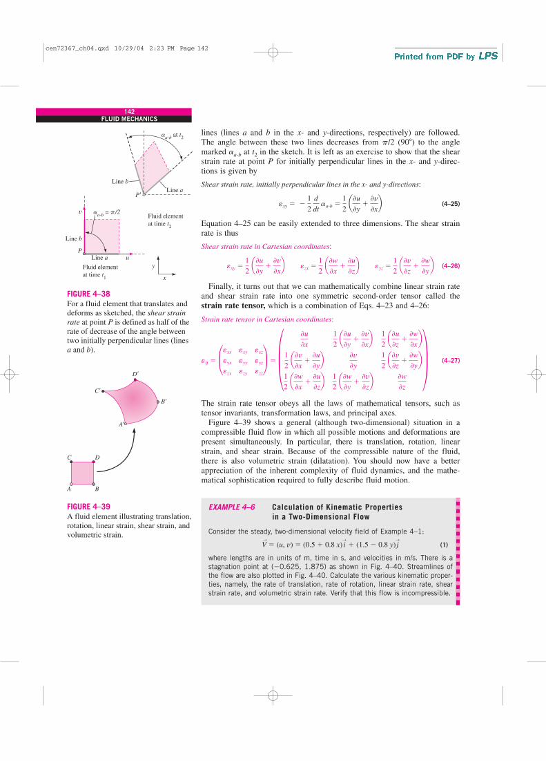
lines (lines a and b in the x- and y-directions, respectively) are followed.

The angle between these two lines decreases from p/2 (90) to the angle

marked aa-b at t2 in the sketch. It is left as an exercise to show that the shear

strain rate at point P for initially perpendicular lines in the x- and y-direc-

tions is given by

Shear strain rate, initially perpendicular lines in the x- and y-directions:

(4–25)

Equation 4–25 can be easily extended to three dimensions. The shear strain

rate is thus

Shear strain rate in Cartesian coordinates:

(4–26)

Finally, it turns out that we can mathematically combine linear strain rate

and shear strain rate into one symmetric second-order tensor called the

strain rate tensor, which is a combination of Eqs. 4–23 and 4–26:

Strain rate tensor in Cartesian coordinates:

(4–27)

The strain rate tensor obeys all the laws of mathematical tensors, such as

tensor invariants, transformation laws, and principal axes.

Figure 4–39 shows a general (although two-dimensional) situation in a

compressible fluid flow in which all possible motions and deformations are

present simultaneously. In particular, there is translation, rotation, linear

strain, and shear strain. Because of the compressible nature of the fluid,

there is also volumetric strain (dilatation). You should now have a better

appreciation of the inherent complexity of fluid dynamics, and the mathe-

matical sophistication required to fully describe fluid motion.

EXAMPLE 4–6 Calculation of Kinematic Properties

in a Two-Dimensional Flow

Consider the steady, two-dimensional velocity field of Example 4–1:

(1)

where lengths are in units of m, time in s, and velocities in m/s. There is a

stagnation point at (�0.625, 1.875) as shown in Fig. 4–40. Streamlines of

the flow are also plotted in Fig. 4–40. Calculate the various kinematic proper-

ties, namely, the rate of translation, rate of rotation, linear strain rate, shear

strain rate, and volumetric strain rate. Verify that this flow is incompressible.

V→

� (u, v) � (0.5 � 0.8 x) i→

� (1.5 � 0.8 y) j→

eij � £exx

eyx

ezx

exy

eyy

ezy

exz

eyz

ezz

≥ � ¶ �u

�x

1

2 a�v

�x�

�u

�yb

1

2 a�w

�x�

�u

�zb

1

2 a�u

�y�

�v

�xb

�v

�y

1

2 a�w

�y�

�v

�zb

1

2 a�u

�z�

�w

�xb

1

2 a�v

�z�

�w

�yb

�w

�z

∂

exy �1

2 a�u

�y�

�v

�xb ezx �

1

2 a�w

�x�

�u

�zb eyz �

1

2 a�v

�z�

�w

�yb

exy � �1

2 d

dt aa-b �

1

2 a�u

�y�

�v

�xb

142FLUID MECHANICS

aa-b

at t2

Line a

Line a u

v

y

x

Fluid element

at time t2

Fluid element

at time t1

Line b

Line b

P�

P

aa-b

= p/2

FIGURE 4–38

For a fluid element that translates and

deforms as sketched, the shear strain

rate at point P is defined as half of the

rate of decrease of the angle between

two initially perpendicular lines (lines

a and b).

C D

A B

C�

D�

A�

B�

FIGURE 4–39

A fluid element illustrating translation,

rotation, linear strain, shear strain, and

volumetric strain.

cen72367_ch04.qxd 10/29/04 2:23 PM Page 142

SOLUTION We are to calculate several kinematic properties of a given

velocity field and verify that the flow is incompressible.

Assumptions 1 The flow is steady. 2 The flow is two-dimensional, implying

no z-component of velocity and no variation of u or v with z.

Analysis By Eq. 4–19, the rate of translation is simply the velocity vector

itself, given by Eq. 1. Thus,

Rate of translation: (2)

The rate of rotation is found from Eq. 4–21. In this case, since w � 0

everywhere, and since neither u nor v vary with z, the only nonzero compo-

nent of rotation rate is in the z-direction. Thus,

Rate of rotation: (3)

In this case, we see that there is no net rotation of fluid particles as they

move about. (This is a significant piece of information, to be discussed in

more detail later in this chapter and also in Chap. 10.)

Linear strain rates can be calculated in any arbitrary direction using Eq.

4–22. In the x-, y-, and z-directions, the linear strain rates of Eq. 4–23 are

(4)

Thus, we predict that fluid particles stretch in the x-direction (positive linear

strain rate) and shrink in the y-direction (negative linear strain rate). This is

illustrated in Fig. 4–41, where we have marked an initially square parcel of

fluid centered at (0.25, 4.25). By integrating Eqs. 2 with time, we calculate

the location of the four corners of the marked fluid after an elapsed time of

1.5 s. Indeed this fluid parcel has stretched in the x-direction and has

shrunk in the y-direction as predicted.

Shear strain rate is determined from Eq. 4–26. Because of the two-

dimensionality, nonzero shear strain rates can occur only in the xy-plane.

Using lines parallel to the x- and y-axes as our initially perpendicular lines,

we calculate exy from Eq. 4–26:

(5)

Thus, there is no shear strain in this flow, as also indicated by Fig. 4–41.

Although the sample fluid particle deforms, it remains rectangular; its initially

90 corner angles remain at 90 throughout the time period of the calculation.

Finally, the volumetric strain rate is calculated from Eq. 4–24:

(6)

Since the volumetric strain rate is zero everywhere, we can say definitively

that fluid particles are neither dilating (expanding) nor shrinking (compress-

ing) in volume. Thus, we verify that this flow is indeed incompressible. In Fig.

4–41, the area of the shaded fluid particle remains constant as it moves and

deforms in the flow field.

Discussion In this example it turns out that the linear strain rates (exx and eyy)

are nonzero, while the shear strain rates (exy and its symmetric partner eyx)

1

V D V

Dt� exx � eyy � ezz � (0.8 � 0.8 � 0) s�1 � 0

exy �1

2 a�u

�y�

�v

�xb �

1

2 (0 � 0) � 0

exx ��u

�x� 0.8 s�1 eyy �

�v

�y� �0.8 s�1 ezz � 0

v→

�1

2 a�v

�x�

�u

�ybk

→

�1

2 (0 � 0)k

→

� 0

u � 0.5 � 0.8x v � 1.5 � 0.8y w � 0

143CHAPTER 4

4

3

2y

1

0

–1

–3 –2 –1 0

x

1

FIGURE 4–40

Streamlines for the velocity field

of Example 4–6. The stagnation

point is indicated by the circle at

x � �0.625 m and y � 1.875 m.

6

5

4y

3

2

1

–1 0 1 2

x

3

FIGURE 4–41

Deformation of an initially square

parcel of marked fluid subjected to

the velocity field of Example 4–6 for

a time period of 1.5 s. The stagnation

point is indicated by the circle at x �

�0.625 m and y � 1.875 m, and

several streamlines are plotted.

cen72367_ch04.qxd 10/29/04 2:23 PM Page 143

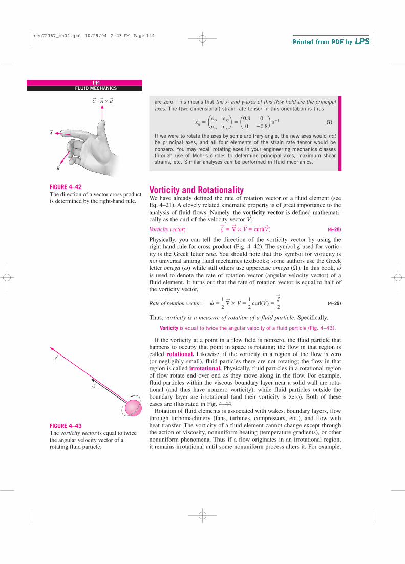
are zero. This means that the x- and y-axes of this flow field are the principal

axes. The (two-dimensional) strain rate tensor in this orientation is thus

(7)

If we were to rotate the axes by some arbitrary angle, the new axes would not

be principal axes, and all four elements of the strain rate tensor would be

nonzero. You may recall rotating axes in your engineering mechanics classes

through use of Mohr’s circles to determine principal axes, maximum shear

strains, etc. Similar analyses can be performed in fluid mechanics.

Vorticity and RotationalityWe have already defined the rate of rotation vector of a fluid element (see

Eq. 4–21). A closely related kinematic property is of great importance to the

analysis of fluid flows. Namely, the vorticity vector is defined mathemati-

cally as the curl of the velocity vector V→

,

Vorticity vector: (4–28)

Physically, you can tell the direction of the vorticity vector by using the

right-hand rule for cross product (Fig. 4–42). The symbol z used for vortic-

ity is the Greek letter zeta. You should note that this symbol for vorticity is

not universal among fluid mechanics textbooks; some authors use the Greek

letter omega (v) while still others use uppercase omega ( ). In this book, v→

is used to denote the rate of rotation vector (angular velocity vector) of a

fluid element. It turns out that the rate of rotation vector is equal to half of

the vorticity vector,

Rate of rotation vector: (4–29)

Thus, vorticity is a measure of rotation of a fluid particle. Specifically,

Vorticity is equal to twice the angular velocity of a fluid particle (Fig. 4–43).

If the vorticity at a point in a flow field is nonzero, the fluid particle that

happens to occupy that point in space is rotating; the flow in that region is

called rotational. Likewise, if the vorticity in a region of the flow is zero

(or negligibly small), fluid particles there are not rotating; the flow in that

region is called irrotational. Physically, fluid particles in a rotational region

of flow rotate end over end as they move along in the flow. For example,

fluid particles within the viscous boundary layer near a solid wall are rota-

tional (and thus have nonzero vorticity), while fluid particles outside the

boundary layer are irrotational (and their vorticity is zero). Both of these

cases are illustrated in Fig. 4–44.

Rotation of fluid elements is associated with wakes, boundary layers, flow

through turbomachinery (fans, turbines, compressors, etc.), and flow with

heat transfer. The vorticity of a fluid element cannot change except through

the action of viscosity, nonuniform heating (temperature gradients), or other

nonuniform phenomena. Thus if a flow originates in an irrotational region,

it remains irrotational until some nonuniform process alters it. For example,

v→

�1

2 §

→

� V→

�1

2 curl(V

→

) �z→

2

z→

� §→

� V→

� curl(V→

)

eij � aexx

eyx

exy

eyy

b � a0.8

0

0

�0.8b s�1

144FLUID MECHANICS

C = A � B

A

B

→ →→

→

→

FIGURE 4–42

The direction of a vector cross product

is determined by the right-hand rule.

z

v→

→

FIGURE 4–43

The vorticity vector is equal to twice

the angular velocity vector of a

rotating fluid particle.

cen72367_ch04.qxd 10/29/04 2:23 PM Page 144

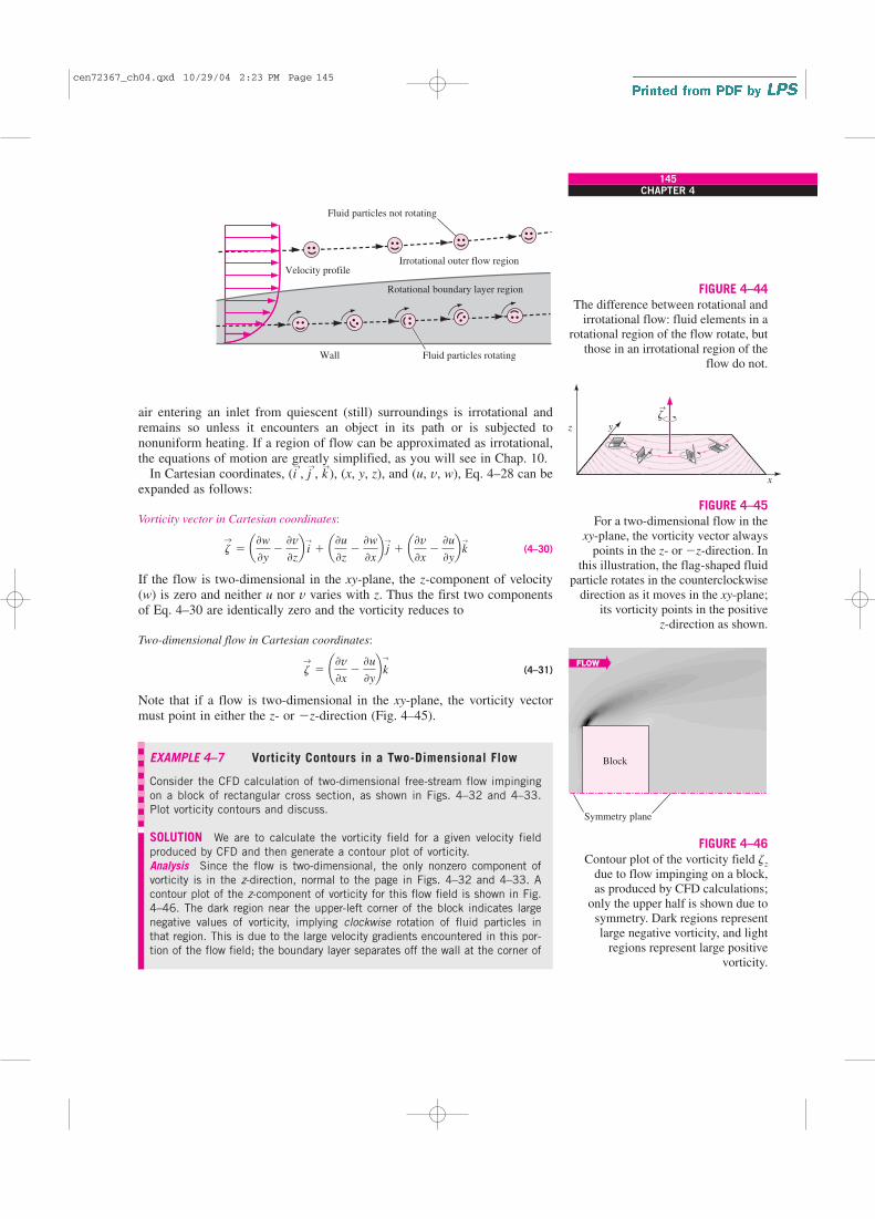
air entering an inlet from quiescent (still) surroundings is irrotational and

remains so unless it encounters an object in its path or is subjected to

nonuniform heating. If a region of flow can be approximated as irrotational,

the equations of motion are greatly simplified, as you will see in Chap. 10.

In Cartesian coordinates, (i→

, j→

, k→

), (x, y, z), and (u, v, w), Eq. 4–28 can be

expanded as follows:

Vorticity vector in Cartesian coordinates:

(4–30)

If the flow is two-dimensional in the xy-plane, the z-component of velocity

(w) is zero and neither u nor v varies with z. Thus the first two components

of Eq. 4–30 are identically zero and the vorticity reduces to

Two-dimensional flow in Cartesian coordinates:

(4–31)

Note that if a flow is two-dimensional in the xy-plane, the vorticity vector

must point in either the z- or �z-direction (Fig. 4–45).

EXAMPLE 4–7 Vorticity Contours in a Two-Dimensional Flow

Consider the CFD calculation of two-dimensional free-stream flow impinging

on a block of rectangular cross section, as shown in Figs. 4–32 and 4–33.

Plot vorticity contours and discuss.

SOLUTION We are to calculate the vorticity field for a given velocity field

produced by CFD and then generate a contour plot of vorticity.

Analysis Since the flow is two-dimensional, the only nonzero component of

vorticity is in the z-direction, normal to the page in Figs. 4–32 and 4–33. A

contour plot of the z-component of vorticity for this flow field is shown in Fig.

4–46. The dark region near the upper-left corner of the block indicates large

negative values of vorticity, implying clockwise rotation of fluid particles in

that region. This is due to the large velocity gradients encountered in this por-

tion of the flow field; the boundary layer separates off the wall at the corner of

z→

� ¢�v

�x�

�u

�y≤k

→

z→

� a�w

�y�

�v

�zb i

→

� a�u

�z�

�w

�xb j

→

� a�v

�x�

�u

�ybk

→

145CHAPTER 4

Fluid particles not rotating

Velocity profileIrrotational outer flow region

Rotational boundary layer region

Fluid particles rotatingWall

FIGURE 4–44

The difference between rotational and

irrotational flow: fluid elements in a

rotational region of the flow rotate, but

those in an irrotational region of the

flow do not.

yz

x

z→

FIGURE 4–45

For a two-dimensional flow in the

xy-plane, the vorticity vector always

points in the z- or �z-direction. In

this illustration, the flag-shaped fluid

particle rotates in the counterclockwise

direction as it moves in the xy-plane;

its vorticity points in the positive

z-direction as shown.

Block

Symmetry plane

FLOW

FIGURE 4–46

Contour plot of the vorticity field zz

due to flow impinging on a block,

as produced by CFD calculations;

only the upper half is shown due to

symmetry. Dark regions represent

large negative vorticity, and light

regions represent large positive

vorticity.

cen72367_ch04.qxd 10/29/04 2:23 PM Page 145

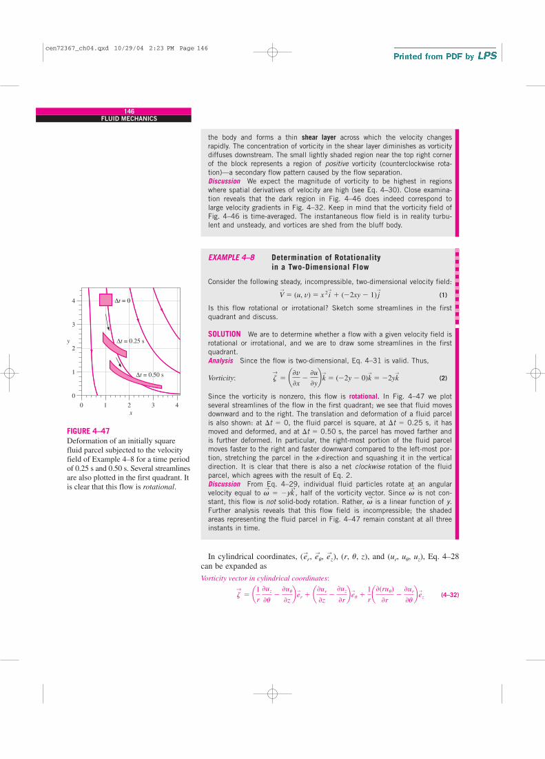
146FLUID MECHANICS

4

3

y

2

1

0

0 1 2 3

x

4

∆t = 0

∆t = 0.25 s

∆t = 0.50 s

FIGURE 4–47

Deformation of an initially square

fluid parcel subjected to the velocity

field of Example 4–8 for a time period

of 0.25 s and 0.50 s. Several streamlines

are also plotted in the first quadrant. It

is clear that this flow is rotational.

the body and forms a thin shear layer across which the velocity changes

rapidly. The concentration of vorticity in the shear layer diminishes as vorticity

diffuses downstream. The small lightly shaded region near the top right corner

of the block represents a region of positive vorticity (counterclockwise rota-

tion)—a secondary flow pattern caused by the flow separation.

Discussion We expect the magnitude of vorticity to be highest in regions

where spatial derivatives of velocity are high (see Eq. 4–30). Close examina-

tion reveals that the dark region in Fig. 4–46 does indeed correspond to

large velocity gradients in Fig. 4–32. Keep in mind that the vorticity field of

Fig. 4–46 is time-averaged. The instantaneous flow field is in reality turbu-

lent and unsteady, and vortices are shed from the bluff body.

EXAMPLE 4–8 Determination of Rotationality

in a Two-Dimensional Flow

Consider the following steady, incompressible, two-dimensional velocity field:

(1)

Is this flow rotational or irrotational? Sketch some streamlines in the first

quadrant and discuss.

SOLUTION We are to determine whether a flow with a given velocity field is

rotational or irrotational, and we are to draw some streamlines in the first

quadrant.

Analysis Since the flow is two-dimensional, Eq. 4–31 is valid. Thus,

Vorticity: (2)

Since the vorticity is nonzero, this flow is rotational. In Fig. 4–47 we plot

several streamlines of the flow in the first quadrant; we see that fluid moves

downward and to the right. The translation and deformation of a fluid parcel

is also shown: at �t � 0, the fluid parcel is square, at �t � 0.25 s, it has

moved and deformed, and at �t � 0.50 s, the parcel has moved farther and

is further deformed. In particular, the right-most portion of the fluid parcel

moves faster to the right and faster downward compared to the left-most por-

tion, stretching the parcel in the x-direction and squashing it in the vertical

direction. It is clear that there is also a net clockwise rotation of the fluid

parcel, which agrees with the result of Eq. 2.

Discussion From Eq. 4–29, individual fluid particles rotate at an angular

velocity equal to v→

� �yk→, half of the vorticity vector. Since v

→is not con-

stant, this flow is not solid-body rotation. Rather, v→

is a linear function of y.

Further analysis reveals that this flow field is incompressible; the shaded

areas representing the fluid parcel in Fig. 4–47 remain constant at all three

instants in time.

In cylindrical coordinates, (e→

r, e→

u, e→

z), (r, u, z), and (ur, uu, uz), Eq. 4–28

can be expanded as

Vorticity vector in cylindrical coordinates:

(4–32)z→

� a1r �uz

�u�

�uu

�zbe

→

r � a�ur

�z�

�uz

�rbe

→

u �1

ra�(ruu)

�r�

�ur

�ube

→

z

z→

� ¢�v

�x�

�u

�y≤k

→

� (�2y � 0)k→

� �2yk→

V→

� (u, v) � x 2 i→

� (�2xy � 1) j→

cen72367_ch04.qxd 10/29/04 2:23 PM Page 146

For two-dimensional flow in the ru-plane, Eq. 4–32 reduces to

Two-dimensional flow in cylindrical coordinates:

(4–33)

where k→

is used as the unit vector in the z-direction in place of e→

z. Note that

if a flow is two-dimensional in the ru-plane, the vorticity vector must point

in either the z- or �z-direction (Fig. 4–48).

Comparison of Two Circular FlowsNot all flows with circular streamlines are rotational. To illustrate this point,

we consider two incompressible, steady, two-dimensional flows, both of

which have circular streamlines in the ru-plane:

Flow A—solid-body rotation: (4–34)

Flow B—line vortex: (4–35)

where v and K are constants. (Alert readers will note that uu in Eq. 4–35 is

infinite at r � 0, which is of course physically impossible; we ignore the

region close to the origin to avoid this problem.) Since the radial component

of velocity is zero in both cases, the streamlines are circles about the origin.

The velocity profiles for the two flows, along with their streamlines, are

sketched in Fig. 4–49. We now calculate and compare the vorticity field for

each of these flows, using Eq. 4–33.

Flow A—solid-body rotation: (4–36)

Flow B—line vortex: (4–37)

Not surprisingly, the vorticity for solid-body rotation is nonzero. In fact, it is

a constant of magnitude twice the angular velocity and pointing in the same

direction. (This agrees with Eq. 4–29.) Flow A is rotational. Physically, this

means that individual fluid particles rotate as they revolve around the origin

(Fig. 4–49a). By contrast, the vorticity of the line vortex is identically zero

everywhere (except right at the origin, which is a mathematical singularity).

Flow B is irrotational. Physically, fluid particles do not rotate as they

revolve in circles about the origin (Fig. 4–49b).

A simple analogy can be made between flow A and a merry-go-round or

roundabout, and flow B and a Ferris wheel (Fig. 4–50). As children revolve

around a roundabout, they also rotate at the same angular velocity as that of

the ride itself. This is analogous to a rotational flow. In contrast, children on

a Ferris wheel always remain oriented in an upright position as they trace

out their circular path. This is analogous to an irrotational flow.

z→

�1

ra�(K)

�r� 0bk

→

� 0

z→

�1

ra�(vr 2)

�r� 0bk

→

� 2vk→

ur � 0 and uu �K

r

ur � 0 and uu � vr

z→

�1

ra�(ruu)

�r�

�ur

�ubk

→

147CHAPTER 4

y

z

x

ru

z→

FIGURE 4–48

For a two-dimensional flow in the

ru-plane, the vorticity vector always

points in the z (or �z) direction. In

this illustration, the flag-shaped fluid

particle rotates in the clockwise

direction as it moves in the ru-plane;

its vorticity points in the �z-direction

as shown.

Flow A uu

uu = vr

r

(a)

Flow B uu

r

(b)

uu = rK

FIGURE 4–49

Streamlines and velocity profiles for

(a) flow A, solid-body rotation and

(b) flow B, a line vortex. Flow A is

rotational, but flow B is irrotational

everywhere except at the origin.

cen72367_ch04.qxd 10/29/04 2:23 PM Page 147

EXAMPLE 4–9 Determination of Rotationality of a Line Sink

A simple two-dimensional velocity field called a line sink is often used to

simulate fluid being sucked into a line along the z-axis. Suppose the volume

flow rate per unit length along the z-axis, V./L, is known, where V

.is a nega-

tive quantity. In two dimensions in the ru-plane,

Line sink: (1)

Draw several streamlines of the flow and calculate the vorticity. Is this flow

rotational or irrotational?

SOLUTION Streamlines of the given flow field are to be sketched and the

rotationality of the flow is to be determined.

Analysis Since there is only radial flow and no tangential flow, we know

immediately that all streamlines must be rays into the origin. Several stream-

lines are sketched in Fig. 4–51. The vorticity is calculated from Eq. 4–33:

(2)

Since the vorticity vector is everywhere zero, this flow field is irrotational.

Discussion Many practical flow fields involving suction, such as flow into

inlets and hoods, can be approximated quite accurately by assuming irrota-

tional flow (Heinsohn and Cimbala, 2003).

4–5 � THE REYNOLDS TRANSPORT THEOREM

In thermodynamics and solid mechanics we often work with a system (also

called a closed system), defined as a quantity of matter of fixed identity. In

fluid dynamics, it is more common to work with a control volume (also

z→

�1

ra�(ruu)

�r�

�

�u urb k

→

�1

ra0 �

�

�u a V#

2pL 1

rbb k

→

� 0

ur �V#

2pL 1

r and uu � 0

148FLUID MECHANICS

FIGURE 4–50

A simple analogy: (a) rotational circular flow is analogous to a roundabout,

while (b) irrotational circular flow is analogous to a Ferris wheel.

© Robb Gregg/PhotoEdit

y

x

Streamlines

u

r

FIGURE 4–51

Streamlines in the ru-plane for the

case of a line sink.

(a) (b)

cen72367_ch04.qxd 10/29/04 2:23 PM Page 148

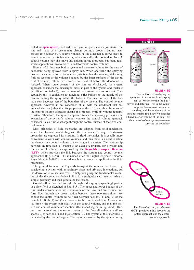
called an open system), defined as a region in space chosen for study. The

size and shape of a system may change during a process, but no mass

crosses its boundaries. A control volume, on the other hand, allows mass to

flow in or out across its boundaries, which are called the control surface. A

control volume may also move and deform during a process, but many real-

world applications involve fixed, nondeformable control volumes.

Figure 4–52 illustrates both a system and a control volume for the case of

deodorant being sprayed from a spray can. When analyzing the spraying

process, a natural choice for our analysis is either the moving, deforming

fluid (a system) or the volume bounded by the inner surfaces of the can (a

control volume). These two choices are identical before the deodorant is

sprayed. When some contents of the can are discharged, the system

approach considers the discharged mass as part of the system and tracks it

(a difficult job indeed); thus the mass of the system remains constant. Con-

ceptually, this is equivalent to attaching a flat balloon to the nozzle of the

can and letting the spray inflate the balloon. The inner surface of the bal-

loon now becomes part of the boundary of the system. The control volume

approach, however, is not concerned at all with the deodorant that has

escaped the can (other than its properties at the exit), and thus the mass of

the control volume decreases during this process while its volume remains

constant. Therefore, the system approach treats the spraying process as an

expansion of the system’s volume, whereas the control volume approach

considers it as a fluid discharge through the control surface of the fixed con-

trol volume.

Most principles of fluid mechanics are adopted from solid mechanics,

where the physical laws dealing with the time rates of change of extensive

properties are expressed for systems. In fluid mechanics, it is usually more

convenient to work with control volumes, and thus there is a need to relate

the changes in a control volume to the changes in a system. The relationship

between the time rates of change of an extensive property for a system and

for a control volume is expressed by the Reynolds transport theorem(RTT), which provides the link between the system and control volume

approaches (Fig. 4–53). RTT is named after the English engineer, Osborne

Reynolds (1842–1912), who did much to advance its application in fluid

mechanics.

The general form of the Reynolds transport theorem can be derived by

considering a system with an arbitrary shape and arbitrary interactions, but

the derivation is rather involved. To help you grasp the fundamental mean-

ing of the theorem, we derive it first in a straightforward manner using a

simple geometry and then generalize the results.

Consider flow from left to right through a diverging (expanding) portion

of a flow field as sketched in Fig. 4–54. The upper and lower bounds of the

fluid under consideration are streamlines of the flow, and we assume uni-

form flow through any cross section between these two streamlines. We

choose the control volume to be fixed between sections (1) and (2) of the

flow field. Both (1) and (2) are normal to the direction of flow. At some ini-

tial time t, the system coincides with the control volume, and thus the sys-

tem and control volume are identical (the shaded region in Fig. 4–54). Dur-

ing time interval �t, the system moves in the flow direction at uniform

speeds V1 at section (1) and V2 at section (2). The system at this later time is

indicated by the hatched region. The region uncovered by the system during

149CHAPTER 4

(a)

Sprayed mass

(b)

System

CV

FIGURE 4–52

Two methods of analyzing the

spraying of deodorant from a spray

can: (a) We follow the fluid as it

moves and deforms. This is the system

approach—no mass crosses the

boundary, and the total mass of the

system remains fixed. (b) We consider

a fixed interior volume of the can. This

is the control volume approach—mass

crosses the boundary.

Control

volume

RTT

System

FIGURE 4–53

The Reynolds transport theorem

(RTT) provides a link between the

system approach and the control

volume approach.

cen72367_ch04.qxd 10/29/04 2:23 PM Page 149

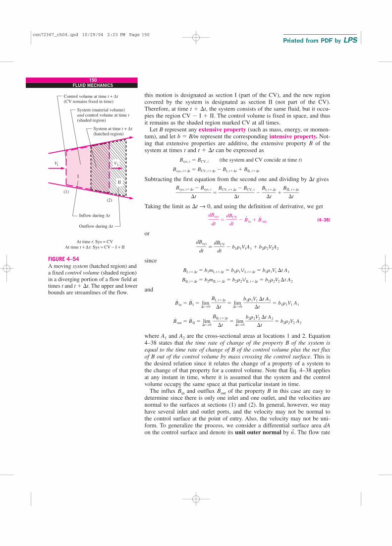
this motion is designated as section I (part of the CV), and the new region

covered by the system is designated as section II (not part of the CV).

Therefore, at time t � �t, the system consists of the same fluid, but it occu-

pies the region CV � I � II. The control volume is fixed in space, and thus

it remains as the shaded region marked CV at all times.

Let B represent any extensive property (such as mass, energy, or momen-

tum), and let b � B/m represent the corresponding intensive property. Not-

ing that extensive properties are additive, the extensive property B of the

system at times t and t � �t can be expressed as

Subtracting the first equation from the second one and dividing by �t gives

Taking the limit as �t → 0, and using the definition of derivative, we get

(4–38)

or

since

and

where A1 and A2 are the cross-sectional areas at locations 1 and 2. Equation

4–38 states that the time rate of change of the property B of the system is

equal to the time rate of change of B of the control volume plus the net flux

of B out of the control volume by mass crossing the control surface. This is

the desired relation since it relates the change of a property of a system to

the change of that property for a control volume. Note that Eq. 4–38 applies

at any instant in time, where it is assumed that the system and the control

volume occupy the same space at that particular instant in time.

The influx B.in and outflux B

.out of the property B in this case are easy to

determine since there is only one inlet and one outlet, and the velocities are

normal to the surfaces at sections (1) and (2). In general, however, we may

have several inlet and outlet ports, and the velocity may not be normal to

the control surface at the point of entry. Also, the velocity may not be uni-

form. To generalize the process, we consider a differential surface area dA

on the control surface and denote its unit outer normal by n→

. The flow rate

B#

out � B#

II � lim�t→0

BII, t��t

�t� lim

�t→0 b2r2V2 �t A2

�t� b2r2V2 A2

B#

in � B#

I � lim�t→0

BI, t��t

�t� lim

�t→0 b1r1V1 �t A1

�t� b1r1V1 A1

BII, t��t � b2mII, t��t � b2r2V II, t��t � b2r2V2 �t A2

BI, t��t � b1mI, t��t � b1r1V I, t��t � b1r1V1 �t A1

dBsys

dt�

dBCV

dt� b1r1V1A1 � b2r2V2A2

dBsys

dt�

dBCV

dt� B#

in � B#

out

Bsys, t��t � Bsys, t

�t�

BCV, t��t � BCV, t

�t�

BI, t��t

�t�

B�, t��t

�t

Bsys, t��t � BCV, t��t � BI, t��t � BII, t��t

Bsys, t � BCV, t (the system and CV concide at time t)

150FLUID MECHANICS

V2

II

Control volume at time t + ∆t

(CV remains fixed in time)

At time t: Sys = CV

At time t + t: Sys = CV � I + II

System (material volume) and control volume at time t (shaded region)

System at time t + ∆t

(hatched region)

Outflow during ∆t

Inflow during ∆t

I

(1)

(2)

V1

∆

FIGURE 4–54

A moving system (hatched region) and

a fixed control volume (shaded region)

in a diverging portion of a flow field at

times t and t � �t. The upper and lower

bounds are streamlines of the flow.

cen72367_ch04.qxd 10/29/04 2:23 PM Page 150

of property b through dA is rbV→

· n→

dA since the dot product V→

· n→

gives the

normal component of the velocity. Then the net rate of outflow through the

entire control surface is determined by integration to be (Fig. 4–55)

(4–39)

An important aspect of this relation is that it automatically subtracts the

inflow from the outflow, as explained next. The dot product of the velocity

vector at a point on the control surface and the outer normal at that point is

, where u is the angle between the velocity

vector and the outer normal, as shown in Fig. 4–56. For u 90, we have

cos u � 0 and thus V→

· n→

� 0 for outflow of mass from the control volume,

and for u � 90, we have cos u 0 and thus V→

· n→

0 for inflow of mass

into the control volume. Therefore, the differential quantity rbV→

· n→

dA is

positive for mass flowing out of the control volume, and negative for mass

flowing into the control volume, and its integral over the entire control sur-

face gives the rate of net outflow of the property B by mass.

The properties within the control volume may vary with position, in gen-

eral. In such a case, the total amount of property B within the control vol-

ume must be determined by integration:

(4–40)

The term dBCV/dt in Eq. 4–38 is thus equal to , and represents

the time rate of change of the property B content of the control volume. A

positive value for dBCV/dt indicates an increase in the B content, and a neg-

ative value indicates a decrease. Substituting Eqs. 4–39 and 4–40 into Eq.

4–38 yields the Reynolds transport theorem, also known as the system-to-

control-volume transformation for a fixed control volume:

RTT, fixed CV: (4–41)

Since the control volume is not moving or deforming with time, the time

derivative on the right-hand side can be moved inside the integral, since the

domain of integration does not change with time. (In other words, it is irrel-

evant whether we differentiate or integrate first.) But the time derivative in

that case must be expressed as a partial derivative (�/�t) since density and

the quantity b may depend on the position within the control volume. Thus,

an alternate form of the Reynolds transport theorem for a fixed control vol-

ume is

Alternate RTT, fixed CV: (4–42)

Equation 4–41 was derived for a fixed control volume. However, many

practical systems such as turbine and propeller blades involve nonfixed con-

trol volumes. Fortunately, Eq. 4–41 is also valid for moving and/or deform-

ing control volumes provided that the absolute fluid velocity V→

in the last

term be replaced by the relative velocity V→

r ,

dBsys

dt� �

CV

�

�t (rb) d V � �

CS

rbV→

� n→ dA

dBsys

dt�

d

dt �

CV

rb dV � �CS

rbV→

� n→ dA

d

dt �

CV

rb dV

BCV � �CV

rb d V

V→

� n→

� �V→

��n→� cos u � �V→

� cos u

B#

net � B#

out � B#

in � �CS

rbV→

� n→

dA (inflow if negative)

151CHAPTER 4

Bnet = Bout – Bin = �CS

rbV � n dA· · ·

Control volume

nMass

entering

outwardnormal

Massleaving

Massleaving

→ →

→

n→

n→

n→

n =→

FIGURE 4–55

The integral of brV→

� n→

dA over the

control surface gives the net amount

of the property B flowing out of the

control volume (into the control

volume if it is negative) per unit time.

If u < 90°, then cos u > 0 (outflow).

If u > 90°, then cos u < 0 (inflow).

If u = 90°, then cos u = 0 (no flow).

n

Outflow:u < 90°

dAn

Inflow:u > 90°

dA

� n = | || n | cos u = V cos u

→

V→

→ →

V

V V

uu

→→

→→

FIGURE 4–56

Outflow and inflow of mass across the

differential area of a control surface.

cen72367_ch04.qxd 10/29/04 2:23 PM Page 151

Relative velocity: (4–43)

where V→

CS is the local velocity of the control surface (Fig. 4–57). The most

general form of the Reynolds transport theorem is thus

RTT, nonfixed CV: (4–44)

Note that for a control volume that moves and/or deforms with time, the

time derivative must be applied after integration, as in Eq. 4–44. As a simple

example of a moving control volume, consider a toy car moving at a con-

stant absolute velocity V→

car � 10 km/h to the right. A high-speed jet of water

(absolute velocity � V→

jet � 25 km/h to the right) strikes the back of the car

and propels it (Fig. 4–58). If we draw a control volume around the car, the

relative velocity is V→

r � 25 � 10 � 15 km/h to the right. This represents

the velocity at which an observer moving with the control volume (moving

with the car) would observe the fluid crossing the control surface. In other

words, V→

r is the fluid velocity expressed relative to a coordinate system

moving with the control volume.

Finally, by application of the Leibnitz theorem, it can be shown that the

Reynolds transport theorem for a general moving and/or deforming control

volume (Eq. 4–44) is equivalent to the form given by Eq. 4–42, which is

repeated here:

Alternate RTT, nonfixed CV: (4–45)

In contrast to Eq. 4–44, the velocity vector V→

in Eq. 4–45 must be taken as

the absolute velocity (as viewed from a fixed reference frame) in order to

apply to a nonfixed control volume.

During steady flow, the amount of the property B within the control vol-

ume remains constant in time, and thus the time derivative in Eq. 4–44

becomes zero. Then the Reynolds transport theorem reduces to

RTT, steady flow: (4–46)

Note that unlike the control volume, the property B content of the system

may still change with time during a steady process. But in this case the

change must be equal to the net property transported by mass across the

control surface (an advective rather than an unsteady effect).

In most practical engineering applications of the RTT, fluid crosses the

boundary of the control volume at a finite number of well-defined inlets and

outlets (Fig. 4–59). In such cases, it is convenient to cut the control surface

directly across each inlet and outlet and replace the surface integral in Eq.

4–44 with approximate algebraic expressions at each inlet and outlet based

on the average values of fluid properties crossing the boundary. We define

ravg, bavg, and Vr, avg as the average values of r, b, and Vr, respectively, across

an inlet or outlet of cross-sectional area A [e.g., ]. The bavg � (1�A) �

A

b dA

dBsys

dt� �

CS

rbV→

r�n→ dA

dBsys

dt� �

CV

��t (rb) dV��

CS

rbV→�n→ dA

dBsys

dt�

d

dt �

CV

rb dV��CS

rbV→

r�n→ dA

V→

r � V→

� V→

CS

152FLUID MECHANICS

CS

= –r

–

→

CSV

→

CSV

→

CS

→

V

→

VV→

V

FIGURE 4–57

Relative velocity crossing a control

surface is found by vector addition

of the absolute velocity of the fluid

and the negative of the local velocity

of the control surface.

Control volume

Absolute reference frame:

Vjet Vcar

Control volume

Relative reference frame:

Vr = Vjet – Vcar

→ →

→→ →

FIGURE 4–58

Reynolds transport theorem applied to

a control volume moving at constant

velocity.

cen72367_ch04.qxd 10/30/04 3:28 PM Page 152

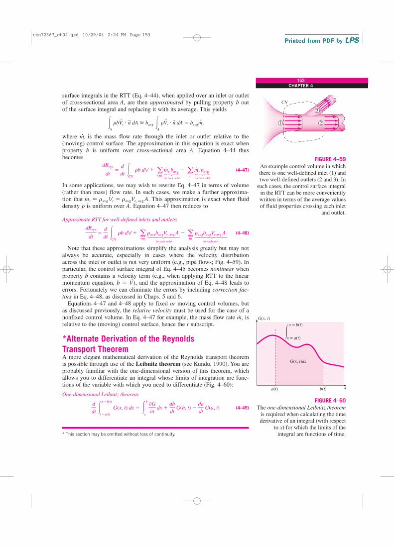
surface integrals in the RTT (Eq. 4–44), when applied over an inlet or outlet

of cross-sectional area A, are then approximated by pulling property b out

of the surface integral and replacing it with its average. This yields

where m.r is the mass flow rate through the inlet or outlet relative to the

(moving) control surface. The approximation in this equation is exact when

property b is uniform over cross-sectional area A. Equation 4–44 thus

becomes

(4–47)

In some applications, we may wish to rewrite Eq. 4–47 in terms of volume

(rather than mass) flow rate. In such cases, we make a further approxima-

tion that . This approximation is exact when fluid

density r is uniform over A. Equation 4–47 then reduces to

Approximate RTT for well-defined inlets and outlets:

(4–48)

Note that these approximations simplify the analysis greatly but may not

always be accurate, especially in cases where the velocity distribution

across the inlet or outlet is not very uniform (e.g., pipe flows; Fig. 4–59). In

particular, the control surface integral of Eq. 4–45 becomes nonlinear when

property b contains a velocity term (e.g., when applying RTT to the linear

momentum equation, b � V→

), and the approximation of Eq. 4–48 leads to

errors. Fortunately we can eliminate the errors by including correction fac-

tors in Eq. 4–48, as discussed in Chaps. 5 and 6.

Equations 4–47 and 4–48 apply to fixed or moving control volumes, but

as discussed previously, the relative velocity must be used for the case of a

nonfixed control volume. In Eq. 4–47 for example, the mass flow rate m.

r is

relative to the (moving) control surface, hence the r subscript.

*Alternate Derivation of the Reynolds

Transport TheoremA more elegant mathematical derivation of the Reynolds transport theorem

is possible through use of the Leibnitz theorem (see Kundu, 1990). You are

probably familiar with the one-dimensional version of this theorem, which

allows you to differentiate an integral whose limits of integration are func-

tions of the variable with which you need to differentiate (Fig. 4–60):

One-dimensional Leibnitz theorem:

(4–49)d

dt �

x�b(t)

x�a(t)

G(x, t) dx � �b

a

�G

�t dx �

db

dt G(b, t) �

da

dt G(a, t)

dBsys

dt�

d

dt �

CV

rb dV � aout

ravgbavgVr, avg A � ain

ravgbavgVr,avg A

m#

r � ravgV#

r � ravgVr, avg A

dBsys

dt�

d

dt �

CV

rb dV � aout

m#

r ˛

bavg � ain

m#

r˛ bavg

�A

rbV→

r � n→ dA � bavg �

A

rV→

r � n→ dA � bavgm

#

r

153CHAPTER 4

CV

1 2

3

FIGURE 4–59

An example control volume in which

there is one well-defined inlet (1) and

two well-defined outlets (2 and 3). In

such cases, the control surface integral

in the RTT can be more conveniently

written in terms of the average values

of fluid properties crossing each inlet

and outlet.

for each outlet for each inlet

for each outlet for each inlet

G(x, t)

xb(t)a(t)

x = b(t)

x = a(t)�

G(x, t)dx

FIGURE 4–60

The one-dimensional Leibnitz theorem

is required when calculating the time

derivative of an integral (with respect

to x) for which the limits of the

integral are functions of time.* This section may be omitted without loss of continuity.

cen72367_ch04.qxd 10/29/04 2:24 PM Page 153

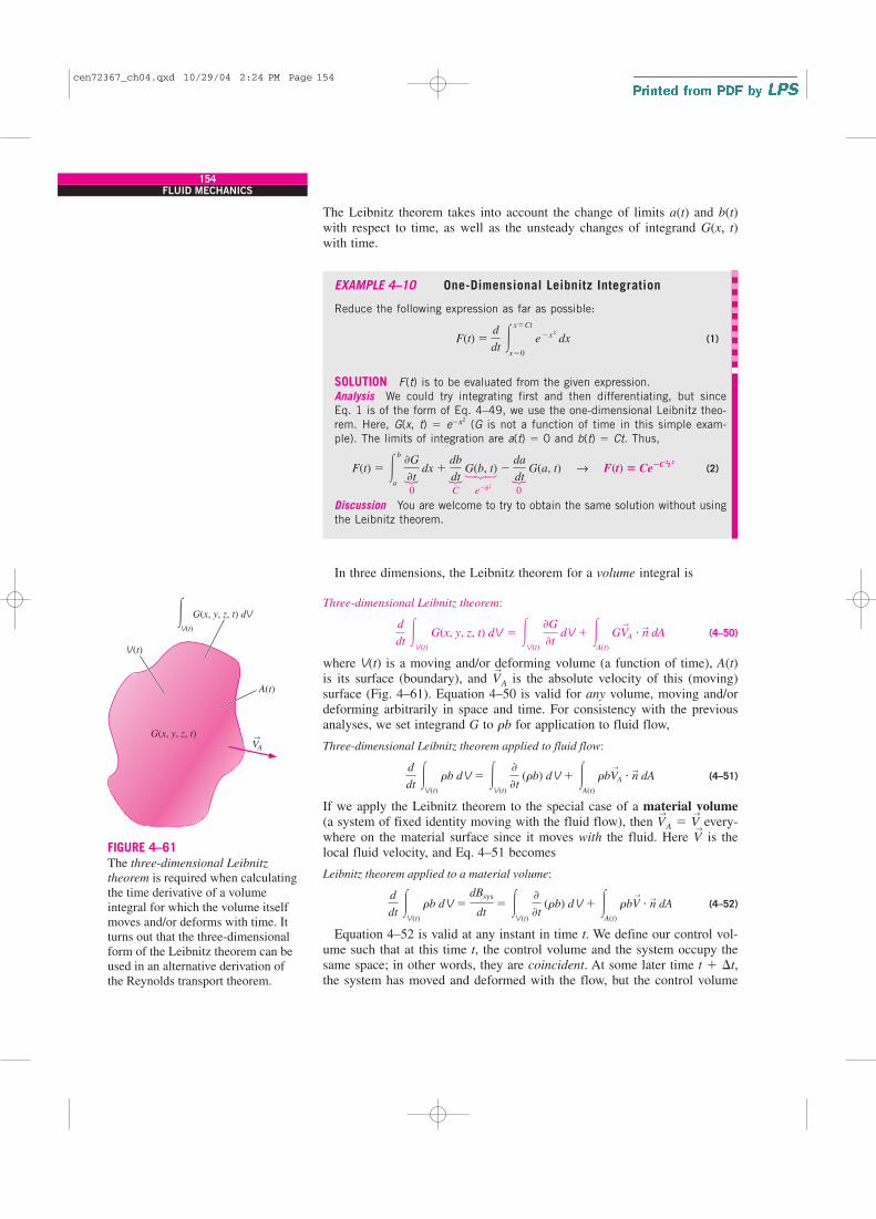
The Leibnitz theorem takes into account the change of limits a(t) and b(t)

with respect to time, as well as the unsteady changes of integrand G(x, t)

with time.

EXAMPLE 4–10 One-Dimensional Leibnitz Integration

Reduce the following expression as far as possible:

(1)

SOLUTION F(t) is to be evaluated from the given expression.

Analysis We could try integrating first and then differentiating, but since

Eq. 1 is of the form of Eq. 4–49, we use the one-dimensional Leibnitz theo-

rem. Here, G(x, t) � e�x2

(G is not a function of time in this simple exam-

ple). The limits of integration are a(t) � 0 and b(t) � Ct. Thus,

(2)

Discussion You are welcome to try to obtain the same solution without using

the Leibnitz theorem.

In three dimensions, the Leibnitz theorem for a volume integral is

Three-dimensional Leibnitz theorem:

(4–50)

where V(t) is a moving and/or deforming volume (a function of time), A(t)

is its surface (boundary), and V→

A is the absolute velocity of this (moving)

surface (Fig. 4–61). Equation 4–50 is valid for any volume, moving and/or

deforming arbitrarily in space and time. For consistency with the previous

analyses, we set integrand G to rb for application to fluid flow,

Three-dimensional Leibnitz theorem applied to fluid flow:

(4–51)

If we apply the Leibnitz theorem to the special case of a material volume(a system of fixed identity moving with the fluid flow), then V

→

A � V→

every-

where on the material surface since it moves with the fluid. Here V→

is the

local fluid velocity, and Eq. 4–51 becomes

Leibnitz theorem applied to a material volume:

(4–52)

Equation 4–52 is valid at any instant in time t. We define our control vol-

ume such that at this time t, the control volume and the system occupy the

same space; in other words, they are coincident. At some later time t � �t,

the system has moved and deformed with the flow, but the control volume

d

dt �

V(t)

rb dV �dBsys

dt� �

V(t)

�

�t (rb) dV � �

A(t)

rbV→

� n→ dA

d

dt �

V(t)

rb dV � �V(t)

�

�t (rb) dV � �

A(t)

rbV→

A � n→ dA

d

dt �

V(t)

G(x, y, z, t) dV � �V(t)

�G

�t dV � �

A(t)

GV→

A � n→ dA

F(t) � �b

a

�G

�t dx �

db

dt G(b, t) �

da

dt G(a, t) → F(t) � Ce�C˛˛

2t 2

F(t) �d

dt �

x�Ct

x�0

e�x2

dx

154FLUID MECHANICS

0 C e�b2

0

F F F

A(t)

V(t)

G(x, y, z, t) d V

G(x, y, z, t)VA

→

V(t)

�

FIGURE 4–61

The three-dimensional Leibnitz

theorem is required when calculating

the time derivative of a volume

integral for which the volume itself

moves and/or deforms with time. It

turns out that the three-dimensional

form of the Leibnitz theorem can be

used in an alternative derivation of

the Reynolds transport theorem.

cen72367_ch04.qxd 10/29/04 2:24 PM Page 154

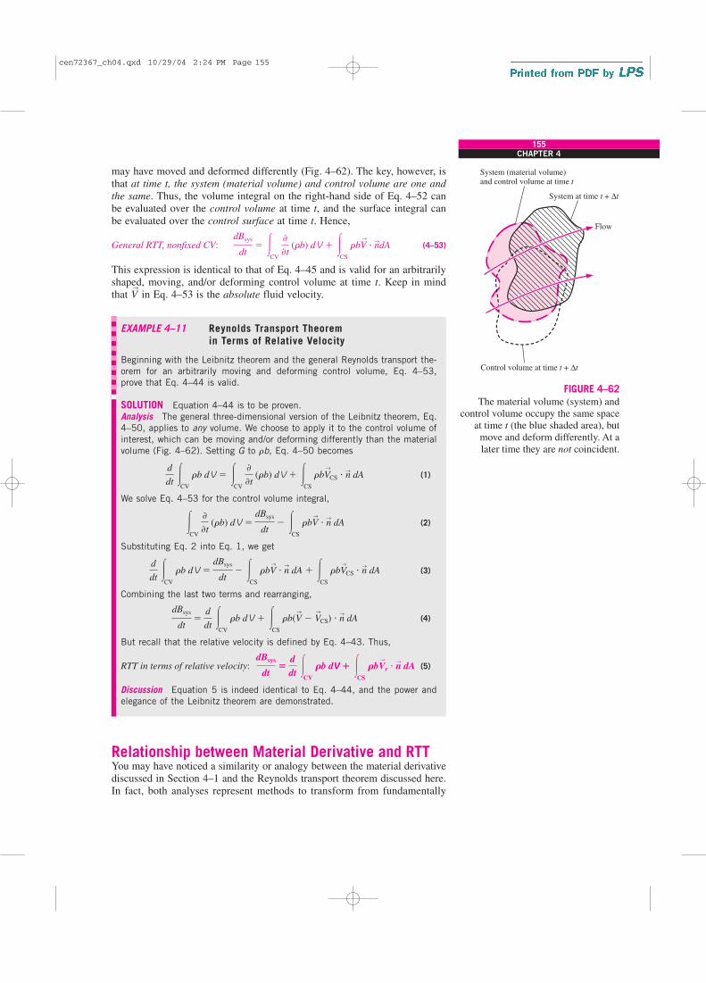
may have moved and deformed differently (Fig. 4–62). The key, however, is

that at time t, the system (material volume) and control volume are one and

the same. Thus, the volume integral on the right-hand side of Eq. 4–52 can

be evaluated over the control volume at time t, and the surface integral can

be evaluated over the control surface at time t. Hence,

General RTT, nonfixed CV: (4–53)

This expression is identical to that of Eq. 4–45 and is valid for an arbitrarily

shaped, moving, and/or deforming control volume at time t. Keep in mind

that V→

in Eq. 4–53 is the absolute fluid velocity.

EXAMPLE 4–11 Reynolds Transport Theorem

in Terms of Relative Velocity

Beginning with the Leibnitz theorem and the general Reynolds transport the-

orem for an arbitrarily moving and deforming control volume, Eq. 4–53,

prove that Eq. 4–44 is valid.

SOLUTION Equation 4–44 is to be proven.

Analysis The general three-dimensional version of the Leibnitz theorem, Eq.

4–50, applies to any volume. We choose to apply it to the control volume of

interest, which can be moving and/or deforming differently than the material

volume (Fig. 4–62). Setting G to rb, Eq. 4–50 becomes

(1)

We solve Eq. 4–53 for the control volume integral,

(2)

Substituting Eq. 2 into Eq. 1, we get

(3)

Combining the last two terms and rearranging,

(4)

But recall that the relative velocity is defined by Eq. 4–43. Thus,

RTT in terms of relative velocity: (5)

Discussion Equation 5 is indeed identical to Eq. 4–44, and the power and

elegance of the Leibnitz theorem are demonstrated.

Relationship between Material Derivative and RTTYou may have noticed a similarity or analogy between the material derivative

discussed in Section 4–1 and the Reynolds transport theorem discussed here.

In fact, both analyses represent methods to transform from fundamentally

dBsys

dt�

d

dt �

CV

Rb dV � �CS

RbV→

r � n→

dA

dBsys

dt�

d

dt �

CV

rb dV � �CS

rb(V→

� V→

CS) � n→ dA

d

dt �

CV

rb dV �dBsys

dt� �

CS

rbV→

� n→

dA � �CS

rbV→

CS � n→ dA

�CV

�

�t (rb) dV �

dBsys

dt� �

CS

rbV→

� n→ dA

d

dt �

CV

rb dV � �CV

�

�t (rb) dV � �

CS

rbV→

CS � n→ dA

dBsys

dt� �

CV

�

�t (rb) dV � �

CS

rbV→

� n→dA

155CHAPTER 4

Flow

System (material volume)and control volume at time t

Control volume at time t + ∆t

System at time t + ∆t

FIGURE 4–62

The material volume (system) and

control volume occupy the same space

at time t (the blue shaded area), but

move and deform differently. At a

later time they are not coincident.

cen72367_ch04.qxd 10/29/04 2:24 PM Page 155

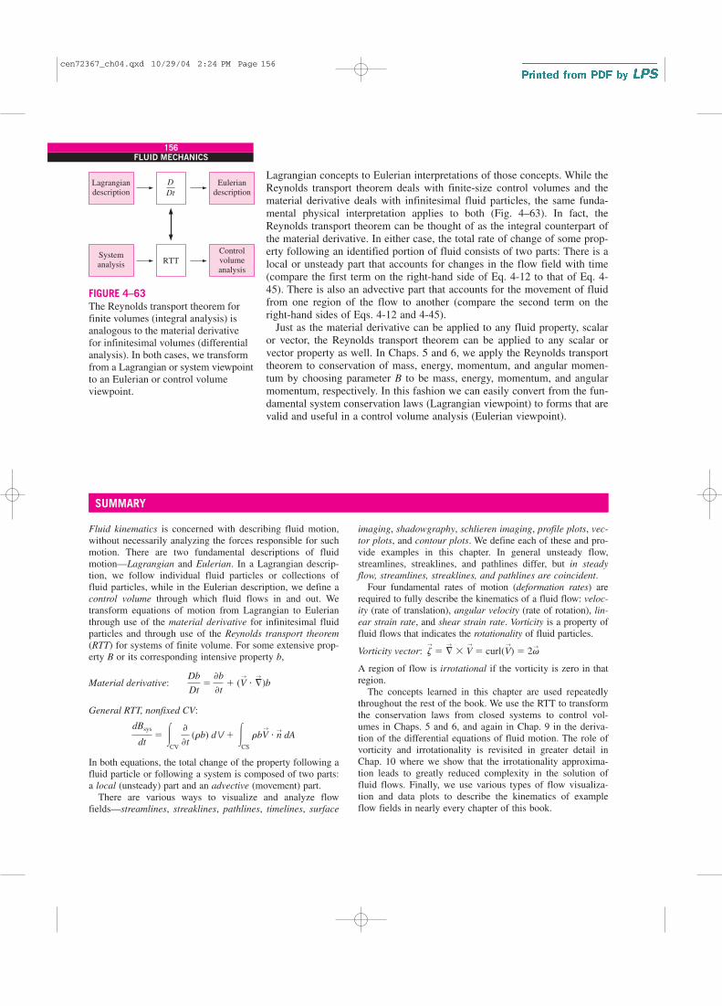
Lagrangian concepts to Eulerian interpretations of those concepts. While the

Reynolds transport theorem deals with finite-size control volumes and the

material derivative deals with infinitesimal fluid particles, the same funda-

mental physical interpretation applies to both (Fig. 4–63). In fact, the

Reynolds transport theorem can be thought of as the integral counterpart of

the material derivative. In either case, the total rate of change of some prop-

erty following an identified portion of fluid consists of two parts: There is a

local or unsteady part that accounts for changes in the flow field with time

(compare the first term on the right-hand side of Eq. 4-12 to that of Eq. 4-

45). There is also an advective part that accounts for the movement of fluid

from one region of the flow to another (compare the second term on the

right-hand sides of Eqs. 4-12 and 4-45).

Just as the material derivative can be applied to any fluid property, scalar

or vector, the Reynolds transport theorem can be applied to any scalar or

vector property as well. In Chaps. 5 and 6, we apply the Reynolds transport

theorem to conservation of mass, energy, momentum, and angular momen-

tum by choosing parameter B to be mass, energy, momentum, and angular

momentum, respectively. In this fashion we can easily convert from the fun-

damental system conservation laws (Lagrangian viewpoint) to forms that are

valid and useful in a control volume analysis (Eulerian viewpoint).

156FLUID MECHANICS

Lagrangiandescription

Euleriandescription

Systemanalysis RTT

Controlvolumeanalysis

D

Dt

FIGURE 4–63

The Reynolds transport theorem for

finite volumes (integral analysis) is

analogous to the material derivative

for infinitesimal volumes (differential

analysis). In both cases, we transform

from a Lagrangian or system viewpoint

to an Eulerian or control volume

viewpoint.

SUMMARY

Fluid kinematics is concerned with describing fluid motion,

without necessarily analyzing the forces responsible for such

motion. There are two fundamental descriptions of fluid

motion—Lagrangian and Eulerian. In a Lagrangian descrip-

tion, we follow individual fluid particles or collections of

fluid particles, while in the Eulerian description, we define a

control volume through which fluid flows in and out. We

transform equations of motion from Lagrangian to Eulerian

through use of the material derivative for infinitesimal fluid

particles and through use of the Reynolds transport theorem

(RTT) for systems of finite volume. For some extensive prop-

erty B or its corresponding intensive property b,

Material derivative:

General RTT, nonfixed CV:

In both equations, the total change of the property following a

fluid particle or following a system is composed of two parts:

a local (unsteady) part and an advective (movement) part.

There are various ways to visualize and analyze flow

fields—streamlines, streaklines, pathlines, timelines, surface

dBsys

dt� �

CV

�

�t (rb) dV � �

CS

rbV→

� n→ dA

Db

Dt�

�b

�t� (V

→

� §→

)b

imaging, shadowgraphy, schlieren imaging, profile plots, vec-

tor plots, and contour plots. We define each of these and pro-

vide examples in this chapter. In general unsteady flow,

streamlines, streaklines, and pathlines differ, but in steady

flow, streamlines, streaklines, and pathlines are coincident.

Four fundamental rates of motion (deformation rates) are

required to fully describe the kinematics of a fluid flow: veloc-

ity (rate of translation), angular velocity (rate of rotation), lin-

ear strain rate, and shear strain rate. Vorticity is a property of

fluid flows that indicates the rotationality of fluid particles.

Vorticity vector:

A region of flow is irrotational if the vorticity is zero in that

region.

The concepts learned in this chapter are used repeatedly

throughout the rest of the book. We use the RTT to transform

the conservation laws from closed systems to control vol-

umes in Chaps. 5 and 6, and again in Chap. 9 in the deriva-

tion of the differential equations of fluid motion. The role of

vorticity and irrotationality is revisited in greater detail in

Chap. 10 where we show that the irrotationality approxima-

tion leads to greatly reduced complexity in the solution of

fluid flows. Finally, we use various types of flow visualiza-

tion and data plots to describe the kinematics of example

flow fields in nearly every chapter of this book.

z→

� §→

� V→

� curl(V→

) � 2v→

cen72367_ch04.qxd 10/29/04 2:24 PM Page 156

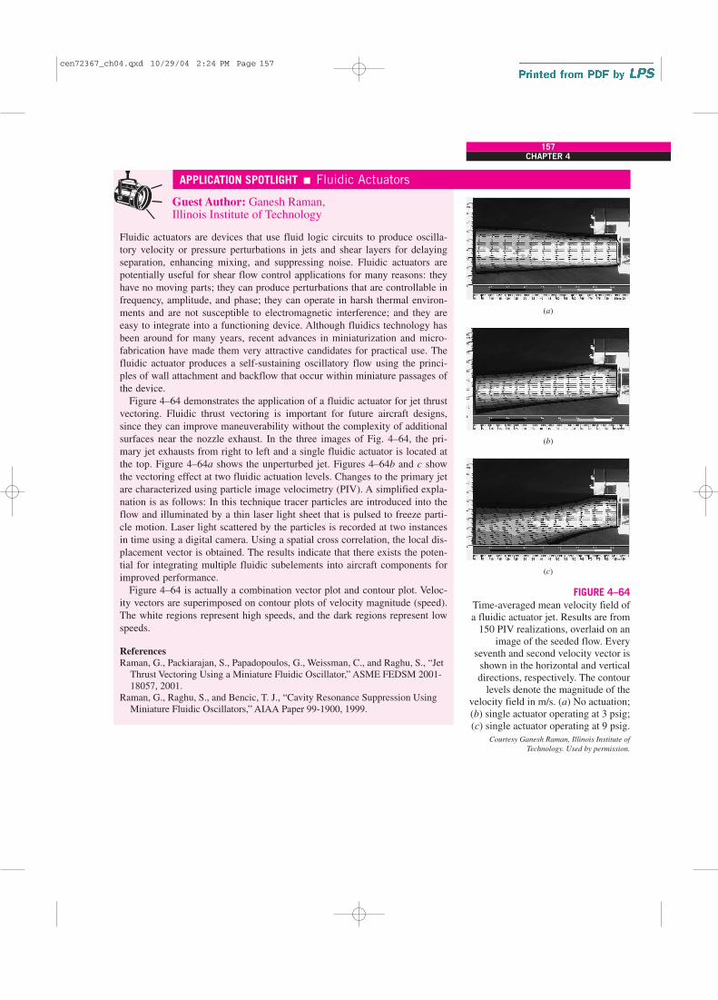
157CHAPTER 4

Guest Author: Ganesh Raman,Illinois Institute of Technology

Fluidic actuators are devices that use fluid logic circuits to produce oscilla-

tory velocity or pressure perturbations in jets and shear layers for delaying

separation, enhancing mixing, and suppressing noise. Fluidic actuators are

potentially useful for shear flow control applications for many reasons: they

have no moving parts; they can produce perturbations that are controllable in

frequency, amplitude, and phase; they can operate in harsh thermal environ-

ments and are not susceptible to electromagnetic interference; and they are

easy to integrate into a functioning device. Although fluidics technology has

been around for many years, recent advances in miniaturization and micro-

fabrication have made them very attractive candidates for practical use. The

fluidic actuator produces a self-sustaining oscillatory flow using the princi-

ples of wall attachment and backflow that occur within miniature passages of

the device.

Figure 4–64 demonstrates the application of a fluidic actuator for jet thrust

vectoring. Fluidic thrust vectoring is important for future aircraft designs,

since they can improve maneuverability without the complexity of additional

surfaces near the nozzle exhaust. In the three images of Fig. 4–64, the pri-

mary jet exhausts from right to left and a single fluidic actuator is located at

the top. Figure 4–64a shows the unperturbed jet. Figures 4–64b and c show

the vectoring effect at two fluidic actuation levels. Changes to the primary jet

are characterized using particle image velocimetry (PIV). A simplified expla-

nation is as follows: In this technique tracer particles are introduced into the

flow and illuminated by a thin laser light sheet that is pulsed to freeze parti-

cle motion. Laser light scattered by the particles is recorded at two instances

in time using a digital camera. Using a spatial cross correlation, the local dis-

placement vector is obtained. The results indicate that there exists the poten-

tial for integrating multiple fluidic subelements into aircraft components for

improved performance.

Figure 4–64 is actually a combination vector plot and contour plot. Veloc-

ity vectors are superimposed on contour plots of velocity magnitude (speed).

The white regions represent high speeds, and the dark regions represent low

speeds.

References

Raman, G., Packiarajan, S., Papadopoulos, G., Weissman, C., and Raghu, S., “Jet

Thrust Vectoring Using a Miniature Fluidic Oscillator,” ASME FEDSM 2001-

18057, 2001.

Raman, G., Raghu, S., and Bencic, T. J., “Cavity Resonance Suppression Using

Miniature Fluidic Oscillators,” AIAA Paper 99-1900, 1999.

APPLICATION SPOTLIGHT � Fluidic Actuators

FIGURE 4–64

Time-averaged mean velocity field of

a fluidic actuator jet. Results are from

150 PIV realizations, overlaid on an

image of the seeded flow. Every

seventh and second velocity vector is

shown in the horizontal and vertical

directions, respectively. The contour

levels denote the magnitude of the

velocity field in m/s. (a) No actuation;

(b) single actuator operating at 3 psig;

(c) single actuator operating at 9 psig.

Courtesy Ganesh Raman, Illinois Institute of

Technology. Used by permission.

(a)

(b)

(c)

cen72367_ch04.qxd 10/29/04 2:24 PM Page 157

158FLUID MECHANICS

REFERENCES AND SUGGESTED READING

1. R. J. Adrian. “Particle-Imaging Technique for

Experimental Fluid Mechanics,” Annual Reviews

in Fluid Mechanics, 23, pp. 261–304, 1991.

2. J. M. Cimbala, H. Nagib, and A. Roshko. “Large

Structure in the Far Wakes of Two-Dimensional Bluff

Bodies,” Journal of Fluid Mechanics, 190, pp. 265–298,

1988.

3. R. J. Heinsohn and J. M. Cimbala. Indoor Air Quality

Engineering. New York: Marcel-Dekker, 2003.

4. P. K. Kundu. Fluid Mechanics. San Diego, CA: Academic

Press, 1990.

5. W. Merzkirch. Flow Visualization, 2nd ed. Orlando, FL:

Academic Press, 1987.

6. G. S. Settles. Schlieren and Shadowgraph Techniques:

Visualizing Phenomena in Transparent Media.

Heidelberg: Springer-Verlag, 2001.

7. M. Van Dyke. An Album of Fluid Motion. Stanford, CA:

The Parabolic Press, 1982.

8. F. M. White. Viscous Fluid Flow, 2nd ed. New York:

McGraw-Hill, 1991.

PROBLEMS*

Introductory Problems

4–1C What does the word kinematics mean? Explain what

the study of fluid kinematics involves.

4–2 Consider steady flow of water through an axisymmetric

garden hose nozzle (Fig. P4–2). Along the centerline of the

nozzle, the water speed increases from uentrance to uexit as

sketched. Measurements reveal that the centerline water

speed increases parabolically through the nozzle. Write an

equation for centerline speed u(x), based on the parameters

given here, from x � 0 to x � L.

4–3 Consider the following steady, two-dimensional veloc-

ity field:

Is there a stagnation point in this flow field? If so, where is it?

Answer: x � �0.417, y � �1.67

4–4 Consider the following steady, two-dimensional veloc-

ity field:

Is there a stagnation point in this flow field? If so, where is it?

Lagrangian and Eulerian Descriptions

4–5C What is the Lagrangian description of fluid motion?

4–6C Is the Lagrangian method of fluid flow analysis more

similar to study of a system or a control volume? Explain.

4–7C What is the Eulerian description of fluid motion?

How does it differ from the Lagrangian description?

4–8C A stationary probe is placed in a fluid flow and mea-

sures pressure and temperature as functions of time at one

V→

� (u, v) � (a2 � (b � cx)2) i→

� (�2cby � 2c2xy) j→

V→

� (u, v) � (0.5 � 1.2x) i→

� (�2.0 � 1.2y) j→

* Problems designated by a “C” are concept questions, and

students are encouraged to answer them all. Problems designated

by an “E” are in English units, and the SI users can ignore them.

Problems with the icon are solved using EES, and complete

solutions together with parametric studies are included on the

enclosed DVD. Problems with the icon are comprehensive in

nature and are intended to be solved with a computer, preferably

using the EES software that accompanies this text.

DexitDentrance

uexituentrance

u(x)

x = Lx = 0

FIGURE P4–2

Flow

Probe

FIGURE P4–8C

cen72367_ch04.qxd 10/29/04 2:24 PM Page 158

CHAPTER 4

159

location in the flow (Fig. P4–8C). Is this a Lagrangian or an

Eulerian measurement? Explain.

4–9C A tiny neutrally buoyant electronic pressure probe is

released into the inlet pipe of a water pump and transmits

2000 pressure readings per second as it passes through the

pump. Is this a Lagrangian or an Eulerian measurement?

Explain.

4–10C A weather balloon is launched into the atmosphere

by meteorologists. When the balloon reaches an altitude

where it is neutrally buoyant, it transmits information about

weather conditions to monitoring stations on the ground (Fig.

P4–10C). Is this a Lagrangian or an Eulerian measurement?

Explain.

4–13C Define a steady flow field in the Eulerian reference

frame. In such a steady flow, is it possible for a fluid particle

to experience a nonzero acceleration?

4–14C List at least three other names for the material deriv-

ative, and write a brief explanation about why each name is

appropriate.

4–15 Consider steady, incompressible, two-dimensional

flow through a converging duct (Fig. P4–15). A simple

approximate velocity field for this flow is

where U0 is the horizontal speed at x � 0. Note that this

equation ignores viscous effects along the walls but is a rea-

sonable approximation throughout the majority of the flow

field. Calculate the material acceleration for fluid particles

passing through this duct. Give your answer in two ways:

(1) as acceleration components ax and ay and (2) as accelera-

tion vector a→

.

V→

� (u, v) � (U0 � bx) i→

� byj→

159CHAPTER 4

Helium-filledweather balloon

Transmittinginstrumentation

FIGURE P4–10C

4–11C A Pitot-static probe can often be seen protruding

from the underside of an airplane (Fig. P4–11C). As the air-

plane flies, the probe measures relative wind speed. Is this a

Lagrangian or an Eulerian measurement? Explain.

Probe

FIGURE P4–11C

4–12C Is the Eulerian method of fluid flow analysis more

similar to study of a system or a control volume? Explain.

y

x

U0

FIGURE P4–15

4–16 Converging duct flow is modeled by the steady,

two-dimensional velocity field of Prob. 4–15. The pressure

field is given by

where P0 is the pressure at x � 0. Generate an expression for

the rate of change of pressure following a fluid particle.

4–17 A steady, incompressible, two-dimensional velocity

field is given by the following components in the xy-plane:

Calculate the acceleration field (find expressions for accelera-

tion components ax and ay), and calculate the acceleration at

the point (x, y) � (�2, 3). Answers: ax � �9.233, ay � 14.37

4–18 A steady, incompressible, two-dimensional velocity

field is given by the following components in the xy-plane:

u � 0.20 � 1.3x � 0.85y v � �0.50 � 0.95x � 1.3y

u � 1.1 � 2.8x � 0.65y v � 0.98 � 2.1x � 2.8y

P � P0 �r

2 B2U0 bx � b2(x 2 � y 2)R

cen72367_ch04.qxd 10/29/04 2:24 PM Page 159

Calculate the acceleration field (find expressions for accelera-

tion components ax and ay) and calculate the acceleration at

the point (x, y) � (1, 2).

4–19 For the velocity field of Prob. 4–2, calculate the fluid

acceleration along the nozzle centerline as a function of x and

the given parameters.

4–20 Consider steady flow of air through the diffuser por-

tion of a wind tunnel (Fig. P4–20). Along the centerline of

the diffuser, the air speed decreases from uentrance to uexit as

sketched. Measurements reveal that the centerline air speed

decreases parabolically through the diffuser. Write an equa-

tion for centerline speed u(x), based on the parameters given

here, from x � 0 to x � L.

160FLUID MECHANICS

4–26C What is the definition of a pathline? What do path-

lines indicate?

4–27C What is the definition of a streakline? How do

streaklines differ from streamlines?

4–28C Consider the visualization of flow over a 15 delta

wing in Fig. P4–28C. Are we seeing streamlines, streaklines,

pathlines, or timelines? Explain.

Dexit

Dentrance

uentrance

u(x)

x = Lx = 0

uexit

FIGURE P4–20

4–21 For the velocity field of Prob. 4–20, calculate the fluid

acceleration along the diffuser centerline as a function of x

and the given parameters. For L � 2.0 m, uentrance � 30.0 m/s,

and uexit � 5.0 m/s, calculate the acceleration at x � 0 and

x � 1.0 m. Answers: 0, �297 m/s2

Flow Patterns and Flow Visualization

4–22C What is the definition of a streamline? What do

streamlines indicate?

4–23 Converging duct flow (Fig. P4–15) is modeled by the

steady, two-dimensional velocity field of Prob. 4–15. Generate

an analytical expression for the flow streamlines.

Answer: y � C/(U0 � bx)

4–24E Converging duct flow is modeled by the steady, two-

dimensional velocity field of Prob. 4–15. For the case in

which U0 � 5.0 ft/s and b � 4.6 s�1, plot several streamlines

from x � 0 ft to 5 ft and y � �3 ft to 3 ft. Be sure to show

the direction of the streamlines.

4–25C Consider the visualization of flow over a 12 cone

in Fig. P4–25C. Are we seeing streamlines, streaklines, path-

lines, or timelines? Explain.

FIGURE P4–25C

Visualization of flow over a 12° cone at a 16° angle of

attack at a Reynolds number of 15,000. The visualization

is produced by colored fluid injected into water from ports

in the body.

Courtesy ONERA. Photograph by Werlé.

FIGURE P4–28C

Visualization of flow over a 15° delta wing at a 20° angle

of attack at a Reynolds number of 20,000. The

visualization is produced by colored fluid injected into

water from ports on the underside of the wing.

Courtesy ONERA. Photograph by Werlé.

4–29C Consider the visualization of ground vortex flow in

Fig. P4–29C. Are we seeing streamlines, streaklines, path-

lines, or timelines? Explain.

cen72367_ch04.qxd 10/29/04 2:24 PM Page 160

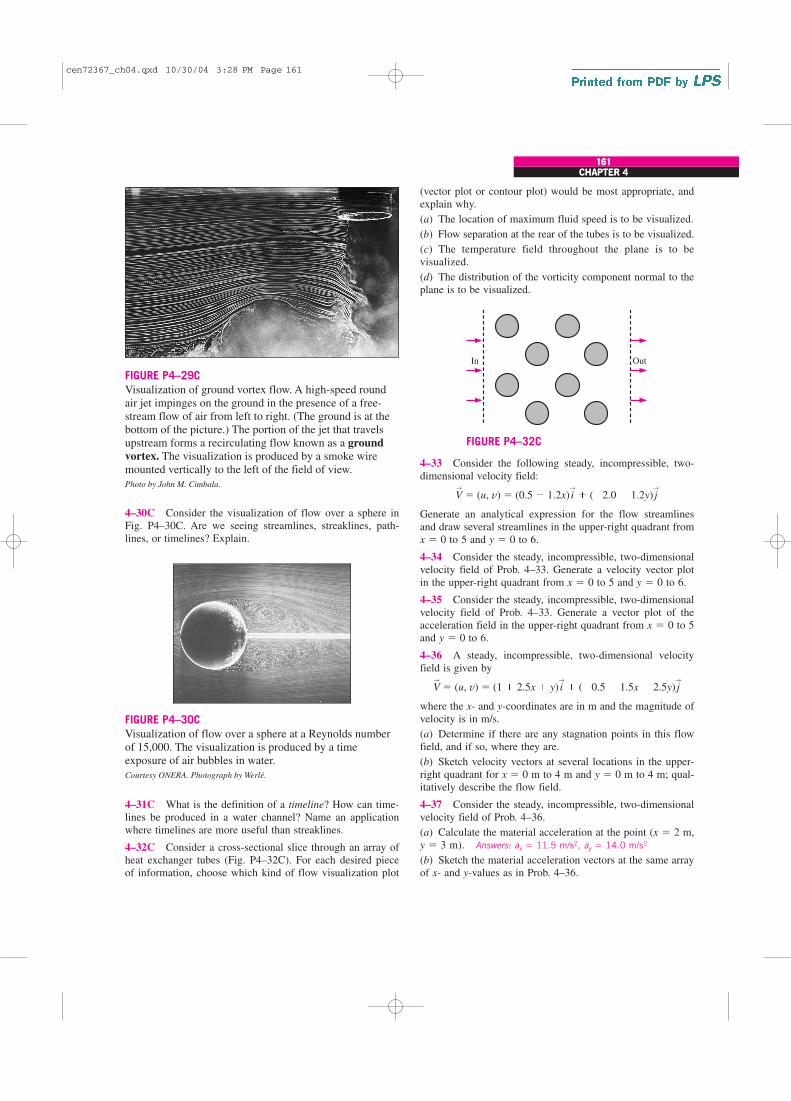
CHAPTER 4

161

4–30C Consider the visualization of flow over a sphere in

Fig. P4–30C. Are we seeing streamlines, streaklines, path-

lines, or timelines? Explain.

(vector plot or contour plot) would be most appropriate, and

explain why.

(a) The location of maximum fluid speed is to be visualized.

(b) Flow separation at the rear of the tubes is to be visualized.

(c) The temperature field throughout the plane is to be

visualized.

(d) The distribution of the vorticity component normal to the

plane is to be visualized.

161CHAPTER 4

FIGURE P4–29C

Visualization of ground vortex flow. A high-speed round

air jet impinges on the ground in the presence of a free-

stream flow of air from left to right. (The ground is at the

bottom of the picture.) The portion of the jet that travels

upstream forms a recirculating flow known as a ground

vortex. The visualization is produced by a smoke wire

mounted vertically to the left of the field of view.

Photo by John M. Cimbala.

FIGURE P4–30C

Visualization of flow over a sphere at a Reynolds number

of 15,000. The visualization is produced by a time

exposure of air bubbles in water.

Courtesy ONERA. Photograph by Werlé.

4–31C What is the definition of a timeline? How can time-

lines be produced in a water channel? Name an application

where timelines are more useful than streaklines.

4–32C Consider a cross-sectional slice through an array of

heat exchanger tubes (Fig. P4–32C). For each desired piece

of information, choose which kind of flow visualization plot

OutIn

FIGURE P4–32C

4–33 Consider the following steady, incompressible, two-

dimensional velocity field:

Generate an analytical expression for the flow streamlines

and draw several streamlines in the upper-right quadrant from

x � 0 to 5 and y � 0 to 6.

4–34 Consider the steady, incompressible, two-dimensional

velocity field of Prob. 4–33. Generate a velocity vector plot

in the upper-right quadrant from x � 0 to 5 and y � 0 to 6.

4–35 Consider the steady, incompressible, two-dimensional

velocity field of Prob. 4–33. Generate a vector plot of the

acceleration field in the upper-right quadrant from x � 0 to 5

and y � 0 to 6.

4–36 A steady, incompressible, two-dimensional velocity

field is given by

where the x- and y-coordinates are in m and the magnitude of

velocity is in m/s.

(a) Determine if there are any stagnation points in this flow

field, and if so, where they are.

(b) Sketch velocity vectors at several locations in the upper-

right quadrant for x � 0 m to 4 m and y � 0 m to 4 m; qual-

itatively describe the flow field.

4–37 Consider the steady, incompressible, two-dimensional

velocity field of Prob. 4–36.

(a) Calculate the material acceleration at the point (x � 2 m,

y � 3 m). Answers: ax � 11.5 m/s2, ay � 14.0 m/s2

(b) Sketch the material acceleration vectors at the same array

of x- and y-values as in Prob. 4–36.

V→

� (u, v) � (1�2.5x�y) i→�(�0.5�1.5x�2.5y) j

→

V→

� (u, v) � (0.5�1.2x) i→�(�2.0�1.2y) j

→

cen72367_ch04.qxd 10/30/04 3:28 PM Page 161

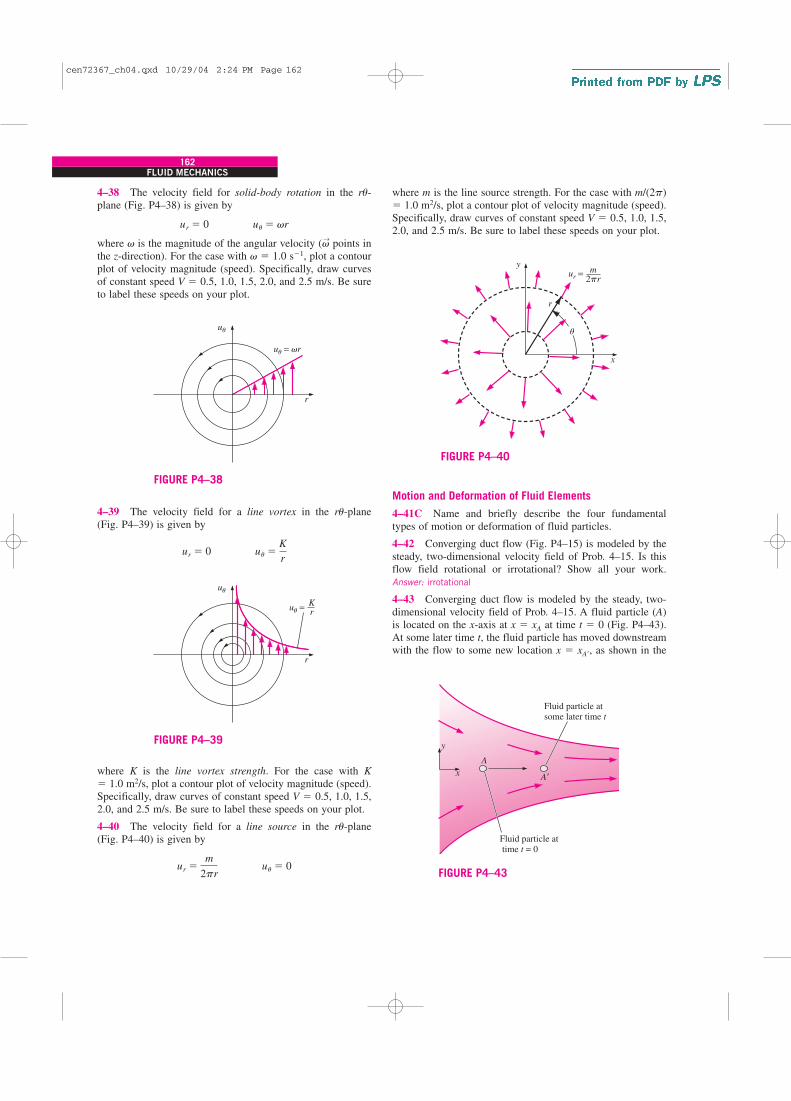
4–38 The velocity field for solid-body rotation in the ru-

plane (Fig. P4–38) is given by

where v is the magnitude of the angular velocity (v→

points in

the z-direction). For the case with v � 1.0 s�1, plot a contour

plot of velocity magnitude (speed). Specifically, draw curves

of constant speed V � 0.5, 1.0, 1.5, 2.0, and 2.5 m/s. Be sure

to label these speeds on your plot.

ur � 0 uu � vr

162FLUID MECHANICS

where m is the line source strength. For the case with m/(2p)

� 1.0 m2/s, plot a contour plot of velocity magnitude (speed).

Specifically, draw curves of constant speed V � 0.5, 1.0, 1.5,

2.0, and 2.5 m/s. Be sure to label these speeds on your plot.

uu

uu = vr

r

FIGURE P4–38

uu

r

uu =Kr

FIGURE P4–39

4–39 The velocity field for a line vortex in the ru-plane

(Fig. P4–39) is given by

ur � 0 uu �K

r

y

x

ur = m 2pr

u

r

FIGURE P4–40

Motion and Deformation of Fluid Elements

4–41C Name and briefly describe the four fundamental

types of motion or deformation of fluid particles.

4–42 Converging duct flow (Fig. P4–15) is modeled by the

steady, two-dimensional velocity field of Prob. 4–15. Is this

flow field rotational or irrotational? Show all your work.

Answer: irrotational

4–43 Converging duct flow is modeled by the steady, two-

dimensional velocity field of Prob. 4–15. A fluid particle (A)

is located on the x-axis at x � xA at time t � 0 (Fig. P4–43).

At some later time t, the fluid particle has moved downstream

with the flow to some new location x � xA�, as shown in the

Fluid particle atsome later time t

Fluid particle at time t = 0

y

A

xA�

FIGURE P4–43

where K is the line vortex strength. For the case with K

� 1.0 m2/s, plot a contour plot of velocity magnitude (speed).

Specifically, draw curves of constant speed V � 0.5, 1.0, 1.5,

2.0, and 2.5 m/s. Be sure to label these speeds on your plot.

4–40 The velocity field for a line source in the ru-plane

(Fig. P4–40) is given by

ur �m

2pr uu � 0

cen72367_ch04.qxd 10/29/04 2:24 PM Page 162

CHAPTER 4

163

figure. Since the flow is symmetric about the x-axis, the fluid

particle remains on the x-axis at all times. Generate an ana-

lytical expression for the x-location of the fluid particle at

some arbitrary time t in terms of its initial location xA and

constants U0 and b. In other words, develop an expression for

xA�. (Hint: We know that u � dxparticle/dt following a fluid par-

ticle. Plug in u, separate variables, and integrate.)

4–44 Converging duct flow is modeled by the steady, two-

dimensional velocity field of Prob. 4–15. Since the flow is

symmetric about the x-axis, line segment AB along the x-axis

remains on the axis, but stretches from length j to length j

� �j as it flows along the channel centerline (Fig. P4–44).

Generate an analytical expression for the change in length of

the line segment, �j. (Hint: Use the result of Prob. 4–43.)

Answer: (xB � xA)(ebt � 1)

163CHAPTER 4

y

A BB�

A�

x

j + ∆jj

FIGURE P4–44

4–45 Using the results from Prob. 4–44 and the fundamen-

tal definition of linear strain rate (the rate of increase in

length per unit length), develop an expression for the linear

strain rate in the x-direction (exx) of fluid particles located on

the centerline of the channel. Compare your result to the gen-

eral expression for exx in terms of the velocity field, i.e., exx

� �u/�x. (Hint: Take the limit as time t → 0. You may need

to apply a truncated series expansion for ebt.) Answer: b

4–46 Converging duct flow is modeled by the steady, two-

dimensional velocity field of Prob. 4–15. A fluid particle (A)

is located at x � xA and y � yA at time t � 0 (Fig. P4–46). At

some later time t, the fluid particle has moved downstream

with the flow to some new location x � xA�, y � yA�, as

shown in the figure. Generate an analytical expression for

the y-location of the fluid particle at arbitrary time t in

terms of its initial y-location yA and constant b. In other

words, develop an expression for yA�. (Hint: We know that v

� dyparticle/dt following a fluid particle. Substitute the equa-

tion for v, separate variables, and integrate.) Answer: yAe�bt

Fluid particle atsome later time t

Fluid particle at time t = 0

yA

A�

x

FIGURE P4–46

h + ∆h

y

A

A�

B�

B

x

h

FIGURE P4–47

4–47 Converging duct flow is modeled by the steady, two-

dimensional velocity field of Prob. 4–15. As vertical line seg-

ment AB moves downstream it shrinks from length h to

length h � �h as sketched in Fig. P4–47. Generate an ana-

lytical expression for the change in length of the line seg-

ment, �h. Note that the change in length, �h, is negative.

(Hint: Use the result of Prob. 4–46.)

4–48 Using the results of Prob. 4–47 and the fundamental

definition of linear strain rate (the rate of increase in length

per unit length), develop an expression for the linear strain

rate in the y-direction (eyy) of fluid particles moving down the

channel. Compare your result to the general expression for

eyy in terms of the velocity field, i.e., eyy � �v/�y. (Hint: Take

the limit as time t → 0. You may need to apply a truncated

series expansion for e�bt.)

4–49E Converging duct flow is modeled by the steady,

two-dimensional velocity field of Prob. 4–15.

For the case in which U0 � 5.0 ft/s and b � 4.6 s�1, consider

an initially square fluid particle of edge dimension 0.5 ft,

centered at x � 0.5 ft and y � 1.0 ft at t � 0 (Fig. P4–49E).

cen72367_ch04.qxd 10/29/04 2:24 PM Page 163

Carefully calculate and plot where the fluid particle will be

and what it will look like at time t � 0.2 s later. Comment on

the fluid particle’s distortion. (Hint: Use the results of Probs.

4–43 and 4–46.)

164FLUID MECHANICS

4–58 Consider steady, incompressible, two-dimensional shear

flow for which the velocity field is

where a and b are constants. Sketched in Fig. P4–58 is a

small rectangular fluid particle of dimensions dx and dy at

time t. The fluid particle moves and deforms with the flow

such that at a later time (t � dt), the particle is no longer rec-

tangular, as also shown in the figure. The initial location of

each corner of the fluid particle is labeled in Fig. P4–58. The

lower-left corner is at (x, y) at time t, where the x-component

of velocity is u � a � by. At the later time, this corner

moves to (x � u dt, y), or

(a) In similar fashion, calculate the location of each of the

other three corners of the fluid particle at time t � dt.

(b) From the fundamental definition of linear strain rate (the

rate of increase in length per unit length), calculate linear

strain rates exx and eyy. Answers: 0, 0

(c) Compare your results with those obtained from the equa-

tions for exx and eyy in Cartesian coordinates, i.e.,

exx ��u

�x eyy �

�v

�y

(x � (a � by) dt, y)

V→

� (u, v) � (a � by) i→

� 0 j→

Initially square fluid particle at t = 0

Unknown shape and location of fluid particle at later time t

y

x?

FIGURE P4–49E

4–50E Based on the results of Prob. 4–49E, verify that the

converging duct flow field is indeed incompressible.

4–51 Converging duct flow is modeled by the steady, two-

dimensional velocity field of Prob. 4–15. Use the equation

for volumetric strain rate to verify that this flow field is

incompressible.

4–52 A general equation for a steady, two-dimensional

velocity field that is linear in both spatial directions (x and y) is

where U and V and the coefficients are constants. Their

dimensions are assumed to be appropriately defined. Calcu-

late the x- and y-components of the acceleration field.

4–53 For the velocity field of Prob. 4–52, what relationship

must exist between the coefficients to ensure that the flow

field is incompressible? Answer: a1 � b2 � 0

4–54 For the velocity field of Prob. 4–52, calculate the lin-

ear strain rates in the x- and y-directions. Answers: a1, b2

4–55 For the velocity field of Prob. 4–52, calculate the

shear strain rate in the xy-plane.

4–56 Combine your results from Probs. 4–54 and 4–55 to

form the two-dimensional strain rate tensor eij in the xy-plane,

Under what conditions would the x- and y-axes be principal

axes? Answer: b1 � a2 � 0

4–57 For the velocity field of Prob. 4–52, calculate the vor-

ticity vector. In which direction does the vorticity vector

point? Answer: (a2 � b1)k→

eij � ¢exx exy

eyx eyy

≤

V→

� (u, v) � (U � a1x � b1y) i→

� (V � a2x � b2y) j→

Particle at time tParticle attime t + dt

y

x

(x + dx, y + dy)

u = a + by

dy

(x + dx, y)

(x, y + dy)

(x, y)

dx dx

dx dx

FIGURE P4–58

4–59 Use two methods to verify that the flow of Prob. 4–58

is incompressible: (a) by calculating the volume of the fluid

particle at both times, and (b) by calculating the volumetric

strain rate. Note that Prob. 4–58 should be completed before

this problem.

4–60 Consider the steady, incompressible, two-dimensional

flow field of Prob. 4–58. Using the results of Prob. 4–58(a),

do the following:

(a) From the fundamental definition of shear strain rate

(half of the rate of decrease of the angle between two initially

perpendicular lines that intersect at a point), calculate shear

cen72367_ch04.qxd 10/29/04 2:24 PM Page 164

CHAPTER 4

165

strain rate exy in the xy-plane. (Hint: Use the lower edge and

the left edge of the fluid particle, which intersect at 90 at the

lower-left corner of the particle at the initial time.)

(b) Compare your results with those obtained from the equa-

tion for exy in Cartesian coordinates, i.e.,

Answers: (a) b/2, (b) b/2

4–61 Consider the steady, incompressible, two-dimensional

flow field of Prob. 4–58. Using the results of Prob. 4–58(a),

do the following:

(a) From the fundamental definition of the rate of rotation

(average rotation rate of two initially perpendicular lines that

intersect at a point), calculate the rate of rotation of the fluid

particle in the xy-plane, vz. (Hint: Use the lower edge and the

left edge of the fluid particle, which intersect at 90 at the

lower-left corner of the particle at the initial time.)

(b) Compare your results with those obtained from the equa-

tion for vz in Cartesian coordinates, i.e.,

Answers: (a) �b/2, (b) �b/2

4–62 From the results of Prob. 4–61,

(a) Is this flow rotational or irrotational?

(b) Calculate the z-component of vorticity for this flow field.

4–63 A two-dimensional fluid element of dimensions dx

and dy translates and distorts as shown in Fig. P4–63 during

the infinitesimal time period dt � t2 � t1. The velocity com-

vz �1

2 ¢�v

�x�

�u

�y≤

exy �1

2 ¢�u

�y�

�v

�x≤

ponents at point P at the initial time are u and v in the x- and

y-directions, respectively. Show that the magnitude of the rate

of rotation (angular velocity) about point P in the xy-plane is

4–64 A two-dimensional fluid element of dimensions dx

and dy translates and distorts as shown in Fig. P4–63 during

the infinitesimal time period dt � t2 � t1. The velocity com-

ponents at point P at the initial time are u and v in the x- and

y-directions, respectively. Consider the line segment PA in

Fig. P4–63, and show that the magnitude of the linear strain

rate in the x-direction is

4–65 A two-dimensional fluid element of dimensions dx

and dy translates and distorts as shown in Fig. P4–63 during

the infinitesimal time period dt � t2 � t1. The velocity com-

ponents at point P at the initial time are u and v in the x- and

y-directions, respectively. Show that the magnitude of the

shear strain rate about point P in the xy-plane is

4–66 Consider a steady, two-dimensional, incompressible

flow field in the xy-plane. The linear strain rate in the x-

direction is 2.5 s�1. Calculate the linear strain rate in the y-

direction.

4–67 A cylindrical tank of water rotates in solid-body rota-

tion, counterclockwise about its vertical axis (Fig. P4–67) at

angular speed n.

� 360 rpm. Calculate the vorticity of fluid

particles in the tank. Answer: 75.4 k→

rad/s

exy �1

2 ¢�u

�y�

�v

�x≤

exx ��u

�x

vz �1

2 ¢�v

�x�

�u

�y≤165

CHAPTER 4

y

x

Fluid elementat time t2

Fluid elementat time t1

Line a

Line b

Line b

Line a

P�

B�

B

dy

dx

A

u

P

v

ab

p/2

aa

A�

FIGURE P4–63

n⋅

Liquid

Free surface

zrrim

r

FIGURE P4–67

cen72367_ch04.qxd 10/29/04 2:24 PM Page 165

4–68 A cylindrical tank of water rotates about its vertical

axis (Fig. P4–67). A PIV system is used to measure the vor-

ticity field of the flow. The measured value of vorticity in the

z-direction is �55.4 rad/s and is constant to within �0.5 per-

cent everywhere that it is measured. Calculate the angular

speed of rotation of the tank in rpm. Is the tank rotating

clockwise or counterclockwise about the vertical axis?

4–69 A cylindrical tank of radius rrim � 0.35 m rotates about

its vertical axis (Fig. P4–67). The tank is partially filled with

oil. The speed of the rim is 2.6 m/s in the counterclockwise

direction (looking from the top), and the tank has been spin-

ning long enough to be in solid-body rotation. For any fluid

particle in the tank, calculate the magnitude of the component

of vorticity in the vertical z-direction. Answer: 15.0 rad/s

4–70C Explain the relationship between vorticity and rota-

tionality.

4–71 Consider a two-dimensional, incompressible flow

field in which an initially square fluid particle moves and

deforms. The fluid particle dimension is a at time t and is

aligned with the x- and y-axes as sketched in Fig. P4–71. At

some later time, the particle is still aligned with the x- and y-

axes, but has deformed into a rectangle of horizontal length

2a. What is the vertical length of the rectangular fluid particle

at this later time?

166FLUID MECHANICS

4–74 Consider fully developed Couette flow—flow between

two infinite parallel plates separated by distance h, with the

top plate moving and the bottom plate stationary as illustrated

in Fig. P4–74. The flow is steady, incompressible, and two-

dimensional in the xy-plane. The velocity field is given by

Is this flow rotational or irrotational? If it is rotational, calcu-

late the vorticity component in the z-direction. Do fluid parti-

cles in this flow rotate clockwise or counterclockwise?

Answers: yes, �V/h, clockwise

V→

� (u, v) � V y

h i

→

� 0 j→

y

x

a

a

FIGURE P4–71

x

yh u =V

y

h

V

FIGURE P4–74

4–75 For the Couette flow of Fig. P4–74, calculate the lin-

ear strain rates in the x- and y-directions, and calculate the

shear strain rate exy.

4–76 Combine your results from Prob. 4–75 to form the

two-dimensional strain rate tensor eij,

Are the x- and y-axes principal axes?

Reynolds Transport Theorem

4–77C True or false: For each statement, choose whether

the statement is true or false and discuss your answer briefly.

(a) The Reynolds transport theorem is useful for transform-

ing conservation equations from their naturally occurring

control volume forms to their system forms.

(b) The Reynolds transport theorem is applicable only to

nondeforming control volumes.

(c) The Reynolds transport theorem can be applied to both

steady and unsteady flow fields.

(d) The Reynolds transport theorem can be applied to both

scalar and vector quantities.

4–78 Consider the general form of the Reynolds transport

theorem (RTT) given by

dBsys

dt�

d

dt �

CV

rb dV � �CS

rbV→

r � n→

dA

eij � ¢exx exy

eyx eyy ≤

4–72 Consider a two-dimensional, compressible flow field

in which an initially square fluid particle moves and deforms.

The fluid particle dimension is a at time t and is aligned with

the x- and y-axes as sketched in Fig. P4–71. At some later

time, the particle is still aligned with the x- and y-axes but

has deformed into a rectangle of horizontal length 1.06a and

vertical length 0.931a. (The particle’s dimension in the z-

direction does not change since the flow is two-dimensional.)

By what percentage has the density of the fluid particle

increased or decreased?

4–73 Consider the following steady, three-dimensional veloc-

ity field:

Calculate the vorticity vector as a function of space (x, y, z).

� (3.0 � 2.0x � y) i→

� (2.0x � 2.0y) j→

� (0.5xy)k→

V→

� (u, v, w)

cen72367_ch04.qxd 10/29/04 2:24 PM Page 166

CHAPTER 4

167

where V→

r is the velocity of the fluid relative to the control

surface. Let Bsys be the mass m of a system of fluid particles.

We know that for a system, dm/dt � 0 since no mass can

enter or leave the system by definition. Use the given equa-

tion to derive the equation of conservation of mass for a con-

trol volume.

4–79 Consider the general form of the Reynolds transport

theorem (RTT) given by Prob. 4–78. Let Bsys be the linear

momentum mV→

of a system of fluid particles. We know that

for a system, Newton’s second law is

Use the equation of Prob. 4–78 and this equation to derive

the equation of conservation of linear momentum for a con-

trol volume.

4–80 Consider the general form of the Reynolds transport

theorem (RTT) given in Prob. 4–78. Let Bsys be the angular

momentum H→

� r→

� mV→

of a system of fluid particles,

where r→

is the moment arm. We know that for a system, con-

servation of angular momentum can be expressed as

where � M→

is the net moment applied to the system. Use the

equation given in Prob. 4–78 and this equation to derive the

equation of conservation of angular momentum for a control

volume.

4–81 Reduce the following expression as far as possible:

(Hint: Use the one-dimensional Leibnitz theorem.) Answer:

Review Problems

4–82 Consider fully developed two-dimensional Poiseuille

flow—flow between two infinite parallel plates separated by

distance h, with both the top plate and bottom plate station-

ary, and a forced pressure gradient dP/dx driving the flow as

illustrated in Fig. P4–82. (dP/dx is constant and negative.)

Be�B2t2

� Ae�A2t2

F(t) �d

dt �

x�Bt

x�At

e�2x2

dx

aM→

�d

dt H→

sys

a F→

� ma→

� mdV

→

dt�

d

dt (mV

→

)sys

The flow is steady, incompressible, and two-dimensional in

the xy-plane. The velocity components are given by

where m is the fluid’s viscosity. Is this flow rotational or irro-

tational? If it is rotational, calculate the vorticity component

in the z-direction. Do fluid particles in this flow rotate clock-

wise or counterclockwise?

4–83 For the two-dimensional Poiseuille flow of Prob. 4–82,

calculate the linear strain rates in the x- and y-directions, and

calculate the shear strain rate exy.

4–84 Combine your results from Prob. 4–83 to form the

two-dimensional strain rate tensor eij in the xy-plane,

Are the x- and y-axes principal axes?

4–85 Consider the two-dimensional Poiseuille flow of

Prob. 4–82. The fluid between the plates is water

at 40C. Let the gap height h � 1.6 mm and the pressure gra-

dient dP/dx � �230 N/m3. Calculate and plot seven path-

lines from t � 0 to t � 10 s. The fluid particles are released

at x � 0 and at y � 0.2, 0.4, 0.6, 0.8, 1.0, 1.2, and 1.4 mm.

4–86 Consider the two-dimensional Poiseuille flow of

Prob. 4–82. The fluid between the plates is

water at 40C. Let the gap height h � 1.6 mm and the pres-

sure gradient dP/dx � �230 N/m3. Calculate and plot seven

streaklines generated from a dye rake that introduces dye

streaks at x � 0 and at y � 0.2, 0.4, 0.6, 0.8, 1.0, 1.2, and

1.4 mm (Fig. P4–86). The dye is introduced from t � 0 to

t � 10 s, and the streaklines are to be plotted at t � 10 s.

eij � ¢exx exy

eyx eyy ≤

u �1

2m dP

dx (y 2 � hy) v � 0

167CHAPTER 4

x

y

u(y)

h

FIGURE P4–82

4–87 Repeat Prob. 4–86 except that the dye is intro-

duced from t � 0 to t � 10 s, and the streaklines

are to be plotted at t � 12 s instead of 10 s.

4–88 Compare the results of Probs. 4–86 and 4–87

and comment about the linear strain rate in the

x-direction.

4–89 Consider the two-dimensional Poiseuille flow of

Prob. 4–82. The fluid between the plates is water

x

y

u(y)Dye rake

h

FIGURE P4–86

cen72367_ch04.qxd 10/29/04 2:24 PM Page 167

at 40C. Let the gap height h � 1.6 mm and the pressure gra-

dient dP/dx � �230 N/m3. Imagine a hydrogen bubble wire

stretched vertically through the channel at x � 0 (Fig. P4–89).

The wire is pulsed on and off such that bubbles are produced

periodically to create timelines. Five distinct timelines are

generated at t � 0, 2.5, 5.0, 7.5, and 10.0 s. Calculate and plot

what these five timelines look like at time t � 12.5 s.

168FLUID MECHANICS

4–92 Combine your results from Prob. 4–91 to form the

axisymmetric strain rate tensor eij,

Are the x- and r-axes principal axes?

4–93 We approximate the flow of air into a vacuum cleaner

attachment by the following velocity components in the cen-

terplane (the xy-plane):

and

where b is the distance of the attachment above the floor, L is

the length of the attachment, and V.

is the volume flow rate of

air being sucked up into the hose (Fig. P4–93). Determine the

location of any stagnation point(s) in this flow field. Answer:

at the origin

v ��V#

y

pL

x 2 � y 2 � b2

x 4 � 2x 2y 2 � 2x 2b2 � y 4 � 2y 2b2 � b4

u ��V#x

pL

x 2 � y 2 � b2

x 4 � 2x 2y 2 � 2x 2b2 � y 4 � 2y 2b2 � b4

eij � aerr

exr

erx

exx

b

x

u(y)H2 wire

hy

FIGURE P4–89

u(r)

D

R

u

r

x

FIGURE P4–90

4–90 Consider fully developed axisymmetric Poiseuille

flow—flow in a round pipe of radius R (diameter D � 2R),

with a forced pressure gradient dP/dx driving the flow as

illustrated in Fig. P4–90. (dP/dx is constant and negative.)

The flow is steady, incompressible, and axisymmetric about

the x-axis. The velocity components are given by

where m is the fluid’s viscosity. Is this flow rotational or irro-

tational? If it is rotational, calculate the vorticity component

in the circumferential (u) direction and discuss the sign of the

rotation.

u �1

4m dP

dx (r 2 � R2) ur � 0 uu � 0

4–91 For the axisymmetric Poiseuille flow of Prob. 4–90,

calculate the linear strain rates in the x- and r-directions, and

calculate the shear strain rate exr. The strain rate tensor in

cylindrical coordinates (r, u, x) and (ur, uu, ux), is

� ¶ �ur

�r

1

2 ar

�

�r auu

rb �

1

r �ur

�ub

1

2 a�ur

�x�

�ux

�rb

1

2 ar

�

�r auu

rb �

1

r �ur

�ub

1

r �uu

�u�

ur

r

1

2 a1

r �ux

�u�

�uu

�xb

1

2 a�ur

�x�

�ux

�rb

1

2 a1

r �ux

�u�

�uu

�xb

�ux

�x

∂ eij � £err

eur

exr

eru

euu

exu

erx

eux

exx

≥

Floor

V

y

L

z x

b

·

FIGURE P4–93

4–94 Consider the vacuum cleaner of Prob. 4–93. For the

case where b � 2.0 cm, L � 35 cm, and V.

� 0.1098 m3/s,

create a velocity vector plot in the upper half of the xy-plane

from x � �3 cm to 3 cm and from y � 0 cm to 2.5 cm. Draw

as many vectors as you need to get a good feel of the flow

field. Note: The velocity is infinite at the point (x, y) � (0,

2.0 cm), so do not attempt to draw a velocity vector at that

point.

4–95 Consider the approximate velocity field given for the

vacuum cleaner of Prob. 4–93. Calculate the flow speed

along the floor. Dust particles on the floor are most likely to

be sucked up by the vacuum cleaner at the location of maxi-

cen72367_ch04.qxd 10/29/04 2:24 PM Page 168

CHAPTER 4

169

mum speed. Where is that location? Do you think the vacuum

cleaner will do a good job at sucking up dust directly below

the inlet (at the origin)? Why or why not?

4–96 Consider a steady, two-dimensional flow field in the

xy-plane whose x-component of velocity is given by

where a, b, and c are constants with appropriate dimensions.

Of what form does the y-component of velocity need to be in

order for the flow field to be incompressible? In other words,

generate an expression for v as a function of x, y, and the

constants of the given equation such that the flow is incom-

pressible. Answer: �2b(x � c)y � f(x)

4–97 There are numerous occasions in which a fairly uni-

form free-stream flow encounters a long circular cylinder

aligned normal to the flow (Fig. P4–97). Examples include air

flowing around a car antenna, wind blowing against a flag

pole or telephone pole, wind hitting electrical wires, and

ocean currents impinging on the submerged round beams that

support oil platforms. In all these cases, the flow at the rear of

the cylinder is separated and unsteady, and usually turbulent.

However, the flow in the front half of the cylinder is much

more steady and predictable. In fact, except for a very thin

boundary layer near the cylinder surface, the flow field may

be approximated by the following steady, two-dimensional

velocity components in the xy- or ru-plane:

ur � V cos ua1 �a2

r 2b uu � �V sin ua1 �

a2

r 2b

u � a � b(x � c)2

4–99 Consider the upstream half (x 0) of the flow

field of Prob. 4–97 (flow over a circular cylin-

der). We introduce a parameter called the stream function c,

which is constant along streamlines in two-dimensional

flows such as the one being considered here (Fig. P4–99).

The velocity field of Prob. 4–97 corresponds to a stream

function given by

(a) Setting c to a constant, generate an equation for a

streamline. (Hint: Use the quadratic rule to solve for r as a

function of u.)

(b) For the particular case in which V � 1.00 m/s and cylinder

radius a � 10.0 cm, plot several streamlines in the upstream

half of the flow (90 u 270). For consistency, plot in

the range �0.4 m x 0 m, �0.2 m y 0.2 m, with

stream function values evenly spaced between �0.16 m2/s

and 0.16 m2/s.

c� V sin uar �a2

rb

169CHAPTER 4

Vy

r = a

r

u

x

FIGURE P4–97

4–100 Consider the flow field of Prob. 4–97 (flow over a

circular cylinder). Calculate the two linear strain rates in the

ru-plane; i.e., calculate err and euu. Discuss whether fluid line

segments stretch (or shrink) in this flow field. (Hint: The

strain rate tensor in cylindrical coordinates is given in Prob.

4–91.)

4–101 Based on your results of Prob. 4–100, discuss the

compressibility (or incompressibility) of this flow. Answer:

flow is incompressible

4–102 Consider the flow field of Prob. 4–97 (flow over a

circular cylinder). Calculate eru, the shear strain rate in the

ru-plane. Discuss whether fluid particles in this flow deform

with shear or not. (Hint: The strain rate tensor in cylindrical

coordinates is given in Prob. 4–91.)

Streamlines

y

x

c4

c3

c2

c1

FIGURE P4–99

Is this flow field rotational or irrotational? Explain.

4–98 Consider the flow field of Prob. 4–97 (flow over a cir-

cular cylinder). Consider only the front half of the flow (x

0). There is one stagnation point in the front half of the

flow field. Where is it? Give your answer in both cylindrical

(r, u) coordinates and Cartesian (x, y) coordinates.

cen72367_ch04.qxd 10/29/04 2:24 PM Page 169

cen72367_ch04.qxd 10/29/04 2:24 PM Page 170