13 February 2017 1

Getting Student Financing Right in the USA:

Lessons from Australia and England1

Nicholas Barr, London School of Economics and Political Science

Bruce Chapman, Australian National University

Lorraine Dearden, University College London and Institute for Fiscal Studies

Susan Dynarski, University of Michigan and NBER

1 Background

The US student loan system has major problems. As Dynarski (2016) points out, US graduates

owe $1.3 trillion in student loans, seven million borrowers are in default and even more are in

arrears. The impact on borrowers is catastrophic. Those of us with experience of the English

or Australian approaches find aspects of the US college loan arrangements difficult to

understand. In contrast, the systems in England and Australia are fundamentally sound because

those countries have taken seriously the principles advocated by US economists such as Milton

Friedman and James Tobin in designing a loan system suitable for students. The answer they

propose is Income Contingent (in US parlance, income-based) Loans (ICLs), the system

adopted successfully in Australia in 1989, New Zealand in 1992 and England in 1998.

Though the income-contingent systems in Australia, New Zealand and England are not perfect,

design problems are largely the result of last-minute political interference and could be easily

fixed. The problems with these systems, however, are small compared with those in the current

US system (Dynarski 2016). This note draws on British and Australian experience over the last

25 years and offers an income-contingent solution to the most serious problems of the current

US student loan system.

Section 2 explains why ICLs are the right model. Section 3 briefly describes the systems in

Australia and England, and section 4 draws out the strengths of those arrangements. That

discussion sets the scene for section 5 which considers the key design elements in an ICL loan

and the considerations that underpin the choice of the parameters of the system. Readers

prepared to take the arguments for income-contingent repayments on trust can proceed directly

to section 5. Section 6 looks at the distributional implications of possible ICL systems and

illustrates one of these systems for graduates at different points of the earnings distribution,

and compares the repayment profiles of these graduates to what occurs under Stafford Loans.

A particular challenge in the US is a high default rate among borrowers who do not graduate

with a BA, either because they drop out or attend sub-baccalaureate institutions. Only about

sixty per cent of students who enrol at a public, baccalaureate-granting institution in the US

have a degree within eight years (see Figure S-4 in Shapiro, et al, 2016). Borrowers who do

not complete a degree earn far less than graduates and are far more likely to default on their

loans. This problem is largely absent in Australia and England, where university admission is

far more selective and it is therefore comparatively rare for students to drop out.

1 We are grateful for helpful comments from participants at two conferences: Restructuring Student Loans:

Lessons from Abroad, Washington DC, 13 June 2016 and the Higher Education Finance Workship, Tongji

University, October 20 2016. Bruce Chapman wishes to acknowledge financial assistance from the Australian

Research Council and the Research School of Economics at the Australian National University.

13 February 2017 2

The benefits of income-contingent loans are greatest for these borrowers, since ICL protects

them from extremely high repayment burdens during times of low earnings.2 While they benefit

from the consumption smoothing aspect of ICLs, the lower repayment rate of these borrowers

adds relatively little to overall costs, since non-graduates borrow far less than graduates.

In Australia and England, student loans are not used to finance sub-baccalaureate education in

either country [SD: YES?].3 In both settings, there are distinct mechanisms for funding students

in baccalaureate and sub-baccalaureate education. While the US could continue to offer loans

for sub-baccalaureate education, it should do so with an expectation of low repayment rates.

2 Why income contingent repayments for student loans?4

INCOME CONTINGENT REPAYMENTS ARE VERY DIFFERENT. We all understand how

conventional mortgage style loans work: they involve a nominal repayment of $X per month

for n years. With a mortgage style loan:

An increase in the interest rates raises monthly nominal repayments.

What is fixed is the duration of the loan; the variable component is the fraction of a

person’s income absorbed by repayments (referred to as the repayment burden).

Because repayments stay the same (in the absence of interest rates changes), the

repayment burden increases if income falls.

In an system income-contingent system, repayments instead are x% of the borrower’s current

income until he/she has repaid the loan. Further, in virtually all ICL systems payments are

taken only after income reaches a threshold (to protect those facing financial stress). Hence, in

an ICL system the variable component is the duration of the loan, which is longer for borrowers

with lower incomes.

Income-contingency turns many standard understandings about student loans upside down:

An increase in the interest rate has no effect on monthly repayments; what changes is

the duration of the loan.

What is fixed is the fraction of a person’s income absorbed by loan repayments.

If a person’s income rises, their repayments increase but their repayment burden cannot

exceed the repayment rate defined in the policy.

For the reasons set out below, an income contingent design is a better fit than a

conventional loan for borrowing to finance human capital.

WHY NOT CONVENTIONAL LOANS? In a prescient and highly readable account, Friedman

(1955) identified the fundamental reason why conventional mortgage-type loans work well

for home loans but not for investment in skills. Friedman identifies two strategic problems in

the market for student loans:

There is a lack of collateral: in contrast with home loans, there is nothing for a bank to

2 Their repayment trajectories will most closely resemble those of the low-income graduates we analyse in the

paper. 3 Australia recently experimented with expanding its loan program to include students at sub-baccalureate

technical institutes. In the wake of extremely high default rates, [BRUCE INSERT] 4 For fuller discussion, see Barr (2012a, Ch. 12; 2012b).

13 February 2017 3

sell if a student defaults on his/her loan; and, again unlike home loans, students can

emigrate, leaving no forwarding address. In addition,

There is asymmetric information: students are better informed than lenders about

whether they aspire to careers in say financial markets or the arts.

The first problem implies excessive risk for borrowers; both problems imply excessive risk for

lenders. As a result, with conventional mortgage-type loans, investment in human capital is too

low. The deterrent applies to all students, but particularly to those from poorer backgrounds

who tend to be (a) less well informed and (b) less able to absorb financial risk.

These market failures imply that to achieve an efficient level of investment in human capital a

loan system needs two elements:

Consumption smoothing: the loan needs to be large enough to provide consumption

smoothing over the course of the loan; and

Insurance: if consumption smoothing is to be effective (that is, people borrow enough

to finance the efficient amount of investment in human capital), the loan needs to

provide an element of insurance against low earnings.

LOANS WITH INCOME CONTINGENT REPAYMENTS. Having identified the capital market

imperfections outlined above, Friedman goes on to point out that,

‘The device adopted to meet the corresponding problem for other risky investments is

equity investment plus limited liability on the part of shareholders. The counterpart for

education would be to “buy” a share in an individual's earning prospects: to advance him

the funds needed to finance his training on condition that he agree to pay the lender a

specified fraction of his future earnings’ (1955, p. 138)

On that basis he advocates loans from government, in return for which

‘The individual would agree in return to pay to the government in each future year x per

cent of his earnings in excess of y dollars for each $1,000 that he gets in this way. This

payment could easily be combined with payment of income tax and so involve a minimum

of additional administrative expense’ (p. 140).

Based on similar thinking, Yale University introduced a system of ICLs in the 1970s. The main

reason why that system failed was that a university lacks a sufficiently robust capacity to collect

repayments, particularly of an income contingent form.

The operation of student loans is analogous to social security and should operate on the same

principles. Pensions redistribute from a person’s younger to her older self; student loans

redistribute from middle years to earlier years.5

DIFFERENT INCOME CONTINGENT DESIGNS. An income contingent mechanism has two

generic forms:

With a graduate tax (as in Friedman), borrowers repay a fraction of their earnings for

life or (say) till retirement. This is equity finance: repayments are contingent on lifetime

income; thus people with higher lifetime earnings repay more in present-value terms.

5 For an early UK proposal in which student loan repayments are linked to social security contributions, see Barr

(1989).

13 February 2017 4

With loans, repayment continues until the borrower has repaid some specified amount,

for example, 100 per cent of the amount borrowed in present value terms. In this design,

income contingency affects the time path of repayments but, except for the lifetime

poor, not the total repayment.

In what follows we concentrate on loan finance since graduate taxes have problems (Barr

2010) and in effect impose an infinite interest rate on the loans of graduates while they work.

DIFFERENT WAYS OF IMPLEMENTING INCOME CONTINGENT REPAYMENTS. Repayments can

be organised in different ways.

Based on current income, as in Australia, New Zealand and the UK. Since repayments

adjust automatically to current earnings, this is the best method so long as a country has

the institutional capacity to implement it effectively;

Based on past income, as in Hungary; and

Through a hybrid arrangement, as in the Netherlands. The Netherlands has a traditional

mortgage-like system, but if a person’s earnings are low, he/she can contact the student

loans administration and request a lower repayment rate. This lacks the benefits of

automaticity.

KEY ELEMENTS IN DESIGN. The core elements of an ICL are:

The repayment rate(s), that is, repayments as a percent of a person’s current income;

The repayment threshold, that is, the level of income at which repayments start;

The interest rate and/or loan surcharge/administrative charge;

A cap on total and/or annual borrowing from the student loan system;

The maximum number of years of repayment, that is, forgiveness after n years;

Conditions for early repayment;

A robust collection mechanism.

We discuss these elements both individually and in terms of their interactions in section 5.

3 How the English and Australian student loan systems work: Tuition6

Universities in the UK and Australia operate in the public sector with tuition charges set by

government. Fee levels have changed considerably over the last 20 years and are currently:

(i) A maximum of GBP 9,000 (USD 12,000) per full-time student year in England,

irrespective of subject, with over 95 per cent of institutions charging this amount;

and

(ii) Between about AUD 6,000 (USD 5,500) and AUD 9,000 (USD 7,000) per full-time

student year in Australia depending on the course studied, there being three tiers

6 What follows considers the case for tuition debts only although the British arrangement also provides means-

tested loans to cover living costs. The administrative arrangements are identical although policy concerns with

respect to interest rate subsidies are more important in a system that covers living costs because the resulting

debt is larger, hence the distortion caused by an interest subsidy greater.

13 February 2017 5

(for example, law and medicine are in the top and arts and humanities the bottom

tiers).

Upon enrolment, domestic students choose between paying tuition up-front or deferring their

obligation through an ICL system. The vast majority (85 per cent in Australia, 90 per cent in

UK) choose to defer, and a student’s debt is recorded and linked to his/her unique social

security/tax file number. When a borrower starts work, employers withhold loan repayments

based on the borrower’s current income in the same way that they withhold social security

payments and income tax. Outstanding debt is recorded and reconciled within a government

agency, which can be the tax authorities or a separate loans administration, such as the UK

Student Loans Company.

In both Australia and the UK, borrowers have no repayment obligation unless their incomes

exceed a certain amount, GBP 21,000 per year (USD 30,000) in Britain and AUD about 57,000

(USD 42,000) per year in Australia. Above these thresholds loan repayments are an increasing

proportion of income, but cannot exceed 9 and 8 per cent of incomes, respectively in Britain

and Australia. When the loans has been fully repaid, employers are informed and repayment

collections cease; the median duration is about 8 years in Australia and about 27 years in Britain

(where average debts are much larger), although the variance is considerable; in Britain all

outstanding loans are forgiven after 30 years, but there is no maximum repayment period in

Australia. Both systems charge interest, and both include an element of interest subsidies, an

issue considered in more depth below.

4 Key conceptual features of the UK and Australian ICL systems

Several critical features of the British and Australian loan arrangements contrast with those in

the USA. The most important are:

REPAYMENT BURDENS. A critical concept is that of the “repayment burden” (RB), the

proportion of a borrower’s income required for loan payments. The most important benefit of

the British and Australian ICL systems is that by design there is a maximum RB of 8 or 9 per

cent. This feature contrasts sharply with the typical situation in the USA, where RBs for an

individual borrower can fluctuate widely and also differ considerably between student debtors,

as noted in Dynarski (2016).

RBs are a crucial aspect of student loan design because they reflect the difficulty or ease of

meeting repayment obligations. With non-ICL systems, for example standard Stafford loans, a

borrower is required to repay a fixed amount each month for 10 years, irrespective of their

financial capacity to do so. Thus borrowers experiencing unemployment or low earnings

through non-graduation (a particularly likely outcome for borrowers who did not complete their

degree from the for-profit sector), face high RBs, causing hardship and in many cases leading

to default. This cannot happen with an ICL loan system and this is the main benefit of such

arrangements.

Chapman and Dearden (2016) present calculations of RBs for BA graduates in the US at

different percentiles in the US earnings distribution. Though most graduates do not experience

difficulties, those in the 10th and 20th centile face serious problems, particularly early in their

careers. With hypothetical illustrations, Chapman and Dearden report RBs of over 100 per cent

for young men and women in the 10th centile of BA earnings at the age of 22; and even those

in the 20th centile face high RBs of over 30% for men and 40% for women early in their career.

13 February 2017 6

These can seriously distort both labour market decisions (whether to work in the public or

private sector, do volunteering, look after family members) and decisions about family

formation (partnership and when to have children) in ways that are neither efficient nor

equitable. Chapman and Dearden (2016) illustrate this with the example of a young female

teacher who has a child.

A central characteristic of ICL loans in the UK and Australia is that such difficulties are ruled

out by design, since both systems provide automatic insurance against low earnings. As a result,

there are no adverse consequences in terms of damaged credit reputation – a major cost for

debtors in the US system. Furthermore, an ICL system minimises (and for some designs

eliminates) the perverse labour market and family formation incentives that face low earners

in the US system.

ADMINISTRATIVE SIMPLICITY. As Dynarski (2016) stresses, while US borrowers can choose

an income-based repayment stream from the plethora of loan options available, the system is

complex for the user and administratively burdensome. For example, being part of the US

income-based arrangement must be negotiated on an annual basis and requires a fairly

sophisticated understanding of the present value of expected loan repayments of different

repayment options. In the UK and Australian systems, in contrast, repayments adjust

automatically; borrowers are not required to navigate through the myriad rules, nor to make

complex decisions about their loan strategies.

Stiglitz (2014) has labelled these advantages “transactional efficiencies” and promotes this

aspect of the British and Australian policies as one of the most important benefits of ICL. The

resulting benefits take two forms:

The marginal cost of collection is small because the system builds on an existing

administrative income-contingent collection apparatus7.

As noted, the benefit for the borrower is that repayments automatically adjust to

financial circumstances.

ACCURACY IN ADJUSTING REPAYMENTS TO CURRENT FINANCIAL CIRCUMSTANCES. ICL

repayments in the UK or Australia accurately reflect a borrower’s current capacity to repay,

since repayments are collected on the basis of the borrower’s current weekly, fortnightly or

monthly income. This aspect is important for the insurance element built into ICLs. This is not

the case in the US variant of income-based repayment since repayments are based on the

previous year’s income rather than current income (Dynarski, 2016).

The distinction between past and current income would be immaterial with stable and

predictable incomes, but that is not the way the world works for borrowers. The incomes of

young people are least stable, and depend significantly on the state of the labour market when

first seeking full-time employment. Thus the US income-based arrangements are not income

contingent for the most important subset of borrowers – those with unstable employment and

income and/or hours of work. Unemployment benefits and tax credits are rightly based on

current circumstance; for the same reasons, the insurance element in ICLs requires repayments

based on current earnings not past earnings.

7 Administrative costs in the Australian and UK systems are about 3 or 4 per cent of the annual revenue

collected (Chapman, 2014).

13 February 2017 7

ICLS GUARANTEE THAT THE REPAYMENT PERIOD IS OPTIMUM FOR ALL GRADUATES. An

implication of the UK and Australian ICLs is that the repayment period for higher-earning

income borrowers will generally be shorter and for low-earning graduates longer.

There is no good economic argument for having a fixed 10 (or indeed 20 or 30 year) term for

student loans. Indeed, the typical US term of 10 years is an outlier compared with student

loans in other countries; for example, in the Canadian mortgage-style student loan system the

repayment period is 18 years. It is efficient if the lifetime of a loan is related to the lifetime of

the asset, hence 3-year car loans and 25-year home loans. Since the benefits of higher

education last throughout a person’s working life, the option of a long repayment duration is

efficient, as well as reducing the risk of default. Note that, as discussed below, a well-

designed ICL allows early repayment if that is what the borrower wishes.

MINIMISING TAXPAYER SUBSIDIES WITH ICL. The extent of taxpayer subsidy associated with

an ICL depends on its design, discussed in section 5.

It is always possible to design an ICL system that is cost neutral. Key variables include a

combination of low loans, real interest rates above the government cost of borrowing, loan

surcharges, lower thresholds, higher repayment rates, longer loan terms, and a healthy labour

market with good earnings growth. Some of these variables can be controlled, others cannot.

A good ICL system should be transparent, easy to understand, with high take up (essential for

the insurance mechanism), easy to access, easy to administer, placing low burden on borrowers

once they enter the labour market, and basing repayments on current earnings.

The UK and Australian experience points to the following conclusions.

ICLs deliver major benefits in terms of consumption smoothing and insurance,

because they eliminate concerns with high repayment burdens and hence largely

eliminate defaults;

Repayments through employer withholding based on current income is the simplest

and cheapest approach for both lender and borrowers;

A system without the complications of reapplication has significant administrative

and conceptual benefits both for government and borrowers; and

The parameters of an ICL are critical design issues, to which we now turn.

5 Designing an ICL system

This section discusses in turn the elements in an income-contingent system noted earlier: the

repayment function (that is, the repayment rate(s) and repayment threshold); the interest rate

on the loan and/or the loan surcharge; the cap on borrowing from the system; forgiveness after

n years; conditions for early repayment; and the collection mechanism.

Student loans have multiple objectives, including consumption smoothing and social mobility

(hence avoiding high repayment burdens), and fiscal parsimony (thus allowing loans to be large

enough to provide good consumption smoothing, and sufficiently widely available to bring

about the efficient level of investment in skills). The choice of parameter values will depend

on:

The relative weights given to these different objectives;

13 February 2017 8

The choice of the other parameters, i.e. the parameters interact with each other;

The size of the loan;

The level, distribution and projected rate of change of graduate earnings;

The tax and benefit regime operating in a country and the tax base;

Political sensitivity connected with real interest rates and surcharges.

THE CHOICE OF REPAYMENT RATE.

In the UK, the 9 percent repayment rate applies only to earnings above the threshold of

GBP 21,000 per year; thus the repayment for someone earning GBP 22,000 per year is

GBP 90, i.e. 9% of GBP 1,000. In Australia, once a borrower’s earnings cross the

threshold of AUD 54,000, a 4% repayment rate applies to all earnings; thus the

repayment for someone earning AUD 55,000 is AUD 2,200, i.e. 4% of AUD 55,000.

Other things equal, the Australian system can have a lower starting repayment rate, but

at the expense of a ‘cliff edge’ as earnings cross the threshold. Australian evidence

suggests that this has behavioural tax reporting effects in the short run (a bunching of

earnings just below the threshold) but this quickly disappears (after just one year).

A higher repayment rate brings in more repayments faster, but creates a larger potential

distortion to labour supply, as labour supply is affected by the marginal tax rate. In the

UK, the repayment rates of 9% means that the increase in the marginal tax rate above

the threshold is 9% for all graduates (until the loan is repaid). In the Australian system

the increase in the marginal tax rate for a $1 increase in salary is extremely high, as

much as several hundred thousand percent under particular assumptions concerning

eventual repayment. This ‘cliff edge’ can be reduced by having more thresholds with

smaller changes in the repayment rates.

THE CHOICE OF REPAYMENT THRESHOLD.

Other things equal, a lower repayment threshold increases repayments, making it

possible, for example, to have a lower repayment rate.

The case for a higher threshold is to avoid the high marginal tax rates faced by many

low earning recipients of income-tested benefits, and to reduce financial stress on low

earners. A higher threshold disentangles student loan repayments from the welfare

system, with both efficiency and equity gains, but reduces revenue.

The choice of threshold depends on the balance between repayment flows and social

concerns, and will depend crucially on the median level of income in a country, the

extent of income inequality, its tax and benefit systems and the efficiency of the tax

collection/employer withholding system.

THE CHOICE OF INTEREST RATE

If a policy aim is to keep taxpayer subsidies small, one approach is an interest rate on

the loan not below the government’s cost of borrowing. An interest rate below the

cost of finance means that no borrower repays in full in present value terms. The

outcome can be expensive in fiscal terms (especially if the government cost of

borrowing is high). However, a lower interest rate may be politically more palatable,

13 February 2017 9

reduce adverse selection8 and is also more progressive in terms of the proportion of

the loan paid by the cohort of borrowers in present value terms across the earnings

distribution. We return to the issue in section 5.2.

If the interest rate is set above the government’s cost of borrowing, borrowers who

repay their loan in full repay more than the cost of their loan in present value terms.

However this is no longer necessarily progressive within the cohort of borrowers

(since the richest graduates repay their loan faster and hence contribute less

proportionately in present value terms).

THE CHOICE OF SURCHARGE

An alternative to a positive real interest rate, or an option alongside a real interest rate,

is a loan surcharge9 A surcharge has the advantage of transparency (unlike compound

real interest rates) and can help to maintain progressivity within the cohort of

borrowers by allowing a real interest rates in a revenue neutral way (due to the

increased revenue from the surcharge).

A disadvantage is that the surcharge, particularly a large surcharge, invites adverse

selection.

THE CHOICE OF CAP ON BORROWING. Loans should be capped for two reasons.

To prevent people borrowing more than they can realistically repay. Thus the choice of

cap should be heavily influenced by the level and expected rate of growth of average

earnings.

To help to contain fee inflation – a relevant consideration if a country (like the US, in

contrast with Australia and the UK) has no cap on tuition fees. In the UK in 2012, when

fees were allowed to rise to GBP9,000 and student loans were allowed to rise

commensurately, virtually all fees went up to GBP9,00010. This was repeated in 2016

when fees for 2017 were allowed to rise to GBP9,250 and all but a handful of

universities raised fees to the maximum level.11

MAXIMUM NUMBER OF YEARS OF REPAYMENT.

In a system with a positive real interest rate, a lower maximum repayment duration is

more progressive (since lower earners are increasingly protected), but at the expense of

less revenue.

The UK, has a maximum repayment duration of 30 years, i.e. any outstanding loan

balance after 30 years is forgiven. In Australia, by contrast, there is no maximum period

of repayment but implicitly is set to be the death of a debtor.

CONDITIONS FOR EARLY REPAYMENT. In a well-designed system, borrowers should be able

to repay early, in part or fully, with no penalty, so that nobody is forced to take longer than

8 See Barr (2012b, pp 485-7). In Australia, the interest rate is 0% real, in New Zealand is is 0% nominal – so

below the government cost of borrowing. Conversely in the UK the interest rate is 3% real and above the

government cost of borrowing.

9 The US Stafford Loan system currently has a loan surcharge of 1.67 percent..

10 See Haroon Chowdry et al. (2012b) and Lorraine Dearden et al. (2014).

11 See https://www.offa.org.uk/access-agreements/.

13 February 2017 10

they wish to repay. A well designed system should have no incentives to repay early and/or

ensure that there is no loss of revenue if there is early repayment.

A ROBUST COLLECTION MECHANISM. As discussed earlier, employer withholding on the basis

of current earnings is (a) cheap, (b) robust in a country like the USA, and (c) essential if the

insurance element in the loan is to be effective. A system as suggested by Dynarski (2016) in

which employer-withholding is done in the same way as is done for social security

contributions, would be ideal.

FUTURE PROOF: A well-designed ICL should be transparent and, as far as possible, future

proof and not easily subjected to political manipulation.

In sum, a good loan scheme has the characteristics summarised in Box 1.

Box 1 Characteristics of a good loan design

INCOME-CONTINGENT REPAYMENTS based on current earnings.

A WRITE-OFF after n years, or at retirement or death.

REPAYMENT THRESHOLD AND REPAYMENT RATE chosen so such that:

A graduate with ‘good’ earnings repays (in PV terms) 100%, or for high earners

perhaps more than 100%, in the latter case with a cap on maximum overpayment (in

present value terms) by any individual.

As far as possible seeks to avoid distortions, e.g. large cliff edges or wedges.

Such a loan is designed to make a loss on people with low lifetime earnings but should seek

to keep the loss on other borrowers low.

Fiscal parsimony of loan design matters, not out of a sense of the purity of the loan, but

because loans that make avoidable losses reduce their capacity to fulfill their core purpose of

facilitating investment in human capital. Expensive loans restrict one or more of:

The number of loans that are made available;

The size of loans;

Student numbers;

The breadth of the loan system, e.g. not covering living costs, or excluding part-time

students, postgraduate students and students in sub-degree tertiary education.

Spending on more powerful pro-access policies, including earlier in the system.

All these problems are particularly detrimental to students from disadvantaged backgrounds

with less access to family support.

FINANCING NON-REPAYMENT. The design question is where the loss on low-earning

borrowers should fall: (a) on the taxpayer, or on the cohort of borrowers through (b) a cohort

risk premium or (c) a surcharge.

With a small loan any of these methods can work.

13 February 2017 11

The larger the loan the greater the marginal loss (the marginal loss on a $10 loan may

be zero, on a $1m loan close to 100%). If loans are large, excessive reliance on any

one method is generally suboptimal.

Taxpayer subsidy: a large fiscal cost (as in the UK loan until 2012), as just

discussed, creates downward pressure on the number and/or size of loans, and

crowds out other beneficial activities;

Risk premium: a large loss requires a substantial risk premium, that is, an

interest rate significantly above the government’s cost of borrowing, risking

adverse selection and creating potential political problems;

Surcharge: a large loss requires a substantial surcharge, again raising the

prospect of adverse selection.

This line of argument suggests that the loss should be covered by a mix of the three

mechanisms, the mix depending on the size of the loan and country specifics.

6 Empirical illustrations for the US

How might such a system work in the USA? In order to assess this, we requires good earning

simulations of future graduates throughout their (simulated) lifetimes. This is the only way to

work out the full cost implications of different ICL designs and the full distributional

implications for borrowers. In the UK, the Department for Education provides simulated

earnings profiles for male and female graduates, which allow anyone to calculate the

implications of different ICL systems for different types of graduates and on government

finances12 under different assumptions. It is very similar to models developed at the Institute

for Fiscal Studies since 200213. In the USA, it would be easy for the government to replicate

these simulated earnings since they have the best sources of longitudinal data (e.g. see Looney

and Yanellis (2014)).

Instead for this paper we take the latest data from the 2015 Current Population Survey. We

focus on Bachelor of Arts (BA) graduates who do not pursue further post-graduate

qualifications. We put these data in 2016 prices and assume real earnings growth of 1% real

per year for all these graduates.

We assume all BA graduates stay in the same earnings percentile throughout their life. This is

simply for illustrative purposes and in no way reflects a typical earnings path for BA

graduates and will exaggerate differences in earnings across the BA graduate distribution but

should be reasonably accurate in comparing the likely broad taxpayer subsidies involved with

different types of ICL systems.14 We begin by looking at the implications of an example ICL

scheme across the distribution of all BA graduates.

12 See https://www.gov.uk/government/publications/simplified-student-loan-repayment-model.

13 See Haroon Chowdrey et al. (2012a).

14 Note that using example individuals and/or assuming that somebody stays in the same centile of the earnings

distribution is not remotely realistic. Studies that have analysed the PSID and/or SIPP data in the US show that

individuals experience transitory and permanent employment and earnings shocks throughout their lives, e.g.

see Low et al. (2010). Moreover, the largest differences between the two systems are for people with the

weakest labour market outcomes. The aim of the example graduates we use in this section is to show that that a

well designed ICL can make a difference in important ways even for a moderately successful graduate. We also

show, that for a successful graduate, revenue streams can accrue faster than with a mortgage-type loan.

13 February 2017 12

We start with (a) a system with a zero real interest rate, and consider its distributional impact

within the cohort of borrowers and the overall taxpayer subsidy. We then show the

distributional implications of reducing taxpayer subsidies via (b) a real interest rate only or

(c) a real interest rate in combination with a loan surcharge.

We then illustrate the essential differences of our ICL system with a Stafford style mortgage

loan using two examples of graduates: a female BA graduate who is assumed to earn around

the 20th centile of the earnings distribution throughout her life, and a male graduate who is

assumed to earn around the 90th centile of the male earnings distribution throughout his life.

These very different experiences have been chosen to illustrate the range of likely earnings

and ICL experiences.

CASE 1: AN EXAMPLE ICL WITH ZERO REAL INTEREST RATE

How might an ICL system work in the US, and what would be the distributional and taxpayer

subsidies involved? As an illustration only, we draw on Chapman et al. (2016) and start with

the following possible ICL parameters for a US system:

(i) A first income repayment threshold of $25,000 per year, and a second threshold

of $40,000 (in reality these would both uprated annually with inflation);

(ii) A flat 3 percent repayment rate on total income above the first threshold and 6

percent for earnings above the second threshold;

(iii) A zero real interest rate (i.e., debt increases with inflation only);

(iv) A loan write-off after 25 years compared to no write-off.

In order to compare the full distributional implications of this ICL as well as the size of the

taxpayer subsidy, we undertake calculate the quantiles of the earnings distribution at every

age using data from the CPS for BA graduates, and smooth these using polynomials in age

(see Chapman and Dearden (2016)). We use these smoothed quantile estimates by age to

estimate the impact across the entire income distribution of BA graduates. For calculating the

taxpayer subsidy, we pool the male and female results using current BA enrolment

proportions taken from the Digest of Education Statistics for 2014.15 We assume 1% real

earnings growth, 1% inflation and that the government cost of borrowing is the 10-year bond

rate plus ¼ of a point.16

A zero real interest rate in an ICL system is always progressive within the cohort of debtors -

it helps the lowest graduate earners the most. This is because those with lower incomes repay

their loans for longer, and the longer a loan with a subsidized interest rate is not fully repaid,

the bigger is the subsidy.

Figure 1 shows the distributional impact (by deciles of the male and female college earning

distribution) of a zero interest rate for our baseline scenario for men and women. We show

the differences when there is debt write off (after 25 years) and no debt write off.

15 Currently 57% of conferred BA students are female and 43% male. See Table 322.20

http://nces.ed.gov/programs/digest/d15/tables/dt15_322.20.asp?current=yes

16 The Stafford interest rate of 3.78 percent per annum nominal is the government cost of borrowing plus 2.05%

points and hence 1.78% points higher than a real interest rate of one percent (assumed in our ICL example) with

one percent inflation.

13 February 2017 13

Figure 1: Proportion of ICL Loan Repaid by Decile of Lifetime Earnings:

zero real interest rate

Overall, this baseline scheme involves a 24% taxpayer subsidy with a write-off, and a 20%

subsidy with no write off. All graduates receive a taxpayer subsidy because there is a zero

(subsidized) real interest rate while at college and below the first threshold from which every

graduate benefits. On average women repay between 72% and 77% in present valua terms,

and men between 82% and 85%. Having a write-off makes the scheme more progressive for

the cohort of borrowers but only affects the bottom three deciles for women and bottom

decile for men.

Having explained earlier the ill effects of excessive taxpayer subsidies, we now consider two

ways of reducing these subsidies and highlight the regressivity with respect to all taxpayers:

increasing the real interest rate above the government cost of borrowing and applying it for

the duration of the loan (including while at college and when earning below the first

threshold); and introducing a loan surcharge.

CASE 2: RAISING THE REAL INTEREST RATE

Figure 2 shows the relationship between the real interest rate and the extent of taxpayer

subsidies for the ICL described above. In contrast with Case 1, the real interest rate applies

from the moment the student takes out the loan, with no subsidy during college or below the

first threshold17. The figure shows that the taxpayer subsidy falls as the real interest rate

increases. From the graph we can see the level of real interest necessary to make this baseline

ICL system cost neutral. This is identified where the lines cross the x axis.

For the loan with no write off it would be 1.7 % real or 2.7% nominal, and with a 25 year

write-off 2.7% real or 3.7% nominal.18 In what follows this is what we define as involving no

17 In Chapman et al. (2016) we also carry out this exercise with a zero real interest rate applying below the

threshold and during college. This increases the 10% taxpayer subsidy real interest rates to 1.5% (no write-off)

and 2.5% (write-off) and the 0% taxpayer subsidy real interest rates to 2.7% (no write-off) and 3.8% (write-off).

This system is more progressive for the cohort of borrowers than the interest rate system illustrated in this paper.

18 This is almost identical to the current Stafford Loan rate of 3.78% nominal.

0

20

40

60

80

1001 2 3 4 5 6 7 8 9

10

All

Per

cen

tage

Rep

aid

Decile of lifetime earnings

Females

Write Off No Write Off

0

20

40

60

80

100

1 2 3 4 5 6 7 8 9

10

All

Per

cen

tage

Rep

aid

Decile of lifetime earnings

Males

Write Off No Write Off

13 February 2017 14

overall taxpayer subsidy.19 It is also easy to see what interest rate would require an average

taxpayer subsidy of 10% (or indeed any other taxpayer subsidy): for this example the real

interest rate could remain at the government cost of borrowing if there is no write-off, or

1.7% real or 2.7% nominal with write-off after 25 years.

Figure 2: Real Interest Rates and Taxpayer subsidies

Note: The real interest rate is assumed to apply as soon as the loan is taken out.

What are the distributional implications of varying the real interest rate? In Figure 3, we

compare the distributional implications of a 10% taxpayer subsidy and 0% taxpayer subsidy

induced by variation in the interest rate.

19 Of course, this ignores administrative and other costs of implementing an ICL system and ignores non-

completers and two year college students. Hence no taxpayer subsidy for the BA group will necessarily involve

a taxpayer subsidy for the student loan system as a whole. It also ignores direct government funding for teaching

and grants.

-0.4

-0.3

-0.2

-0.1

0

0.1

0.2

0.3

0 0.5 1 1.5 2 2.5 3 3.5 4

Su

bsi

dy

Interest Rate

No write off

Write off

13 February 2017 15

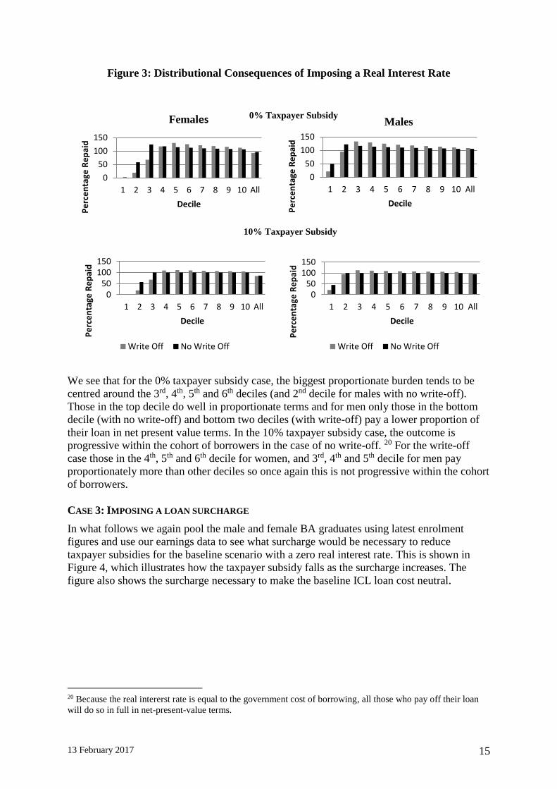
Figure 3: Distributional Consequences of Imposing a Real Interest Rate

We see that for the 0% taxpayer subsidy case, the biggest proportionate burden tends to be

centred around the 3rd, 4th, 5th and 6th deciles (and 2nd decile for males with no write-off).

Those in the top decile do well in proportionate terms and for men only those in the bottom

decile (with no write-off) and bottom two deciles (with write-off) pay a lower proportion of

their loan in net present value terms. In the 10% taxpayer subsidy case, the outcome is

progressive within the cohort of borrowers in the case of no write-off. 20 For the write-off

case those in the 4th, 5th and 6th decile for women, and 3rd, 4th and 5th decile for men pay

proportionately more than other deciles so once again this is not progressive within the cohort

of borrowers.

CASE 3: IMPOSING A LOAN SURCHARGE

In what follows we again pool the male and female BA graduates using latest enrolment

figures and use our earnings data to see what surcharge would be necessary to reduce

taxpayer subsidies for the baseline scenario with a zero real interest rate. This is shown in

Figure 4, which illustrates how the taxpayer subsidy falls as the surcharge increases. The

figure also shows the surcharge necessary to make the baseline ICL loan cost neutral.

20 Because the real intererst rate is equal to the government cost of borrowing, all those who pay off their loan

will do so in full in net-present-value terms.

0

50

100

150

1 2 3 4 5 6 7 8 9 10 All

Pe

rce

nta

ge R

ep

aid

Decile

Females

Write Off No Write Off

050

100150

1 2 3 4 5 6 7 8 9 10 All

Pe

rce

nta

ge R

ep

aid

Decile

Female

Write Off No Write Off

0

50

100

150

1 2 3 4 5 6 7 8 9 10 All

Pe

rce

nta

ge R

ep

aid

Decile

Males

Write Off No Write Off

050

100150

1 2 3 4 5 6 7 8 9 10 All

Pe

rce

nta

ge R

ep

aid

Decile

Male

Write Off No Write Off

0% Taxpayer Subsidy

10% Taxpayer Subsidy

13 February 2017 16

Figure 4: Loan Surcharge and Taxpayer Subsidies: zero real interest rate

Figure 4 shows that a surcharge of around 27% is necessary to avoid any taxpayer subsidy

with no write off, and around 35% with a write off. Alternatively, a surcharge of around 13%

with no write off and 20% with a write-off would require a 10% taxpayer subsidy.

Figure 5: Distributional Consequences of Imposing a Surcharge

-40%

-30%

-20%

-10%

0%

10%

20%

30%

0 5 10 15 20 25 30 35 40 45 50 55 60 65 70 75 80

Su

bsi

dy

Surcharge Percent

Write Off

No Write Off

0

100

200

1 2 3 4 5 6 7 8 9 10 All

Pe

rcen

tage

Re

pai

d

Decile of lifteime earnings

Female

Write Off No Write Off

0

100

200

1 2 3 4 5 6 7 8 9 10 All

Pe

rcen

tage

Re

pai

d

Decile of lifetime earnings

Male

Write Off No Write Off

050

100150

1 2 3 4 5 6 7 8 9 10 All

Pe

rcen

tage

Re

pai

d

Decile

Female 10%

Write Off No Write Off

050

100150

1 2 3 4 5 6 7 8 9 10 All

Pe

rce

nta

ge R

ep

aid

Decile

Male

Write Off No Write Off

0% Taxpayer Subsidy

10% Taxpayer Subsidy

13 February 2017 17

Figure 5 shows the distributional implications of these two surcharges and shows that they

are both progressive within the cohort of borrowers i.e. as we move up the deciles of the

income distribution, graduates pay proportionately more. For each taxpayer subsidy they are

more progressive than the fiscally equivalent interest rate scenario illustrated above. With a

surcharge, the richest graduates pay around 127% of their loan in NPV terms in the case with

no taxpayer subsidy and 113% with a 10% taxpayer subsidy. For a Stafford Loan for the

same amount, the equivalent figure is 114% but this applies to all graduates regardless of

earnings and ignoring default.

Finally, in Figure 6, we show the implications of a hybrid scheme which charges a real

interest rate of 1% above the threshold combined with a surcharge to make up the shortfall.

For a 0% taxpayer subsidy, the surcharge needs to be 16% with no write-off and 25% with a

write off. Alternatively, a surcharge of around 4% with no write off and 10% with a write-off

requires a taxpayer subsidy of 10%.

In these examples, we have shown the implications only of changing real interest rates and

surcharges. However, as highlighted earlier, these are not the only parameters that can be

changed. The implications of changing other parameters are shown in Chapman et. al.

(2016). Importantly, the economic and political implications of charging a surcharge vs

higher real interest rates are different and may differently affect student’s borrowing and

decisions about university. It also depends on how they interact with other components of the

ICL design, the tax and benefit system, the private loan market, and the moral hazard and

adverse selection issues associated with the ICL design.

Figure 6: Distributional Consequences of Imposing a Surcharge: 1% interest rate above

threshold

0

50

100

150

1 2 3 4 5 6 7 8 9 10 All

Pe

rce

nta

ge R

ep

aid

Decile

Females

Write Off No Write Off

0

50

100

150

1 2 3 4 5 6 7 8 9 10 All

Pe

rce

nta

ge R

ep

aid

Decile

Female

Write Off No Write Off

0

50

100

150

1 2 3 4 5 6 7 8 9 10 All

Pe

rce

nta

ge R

ep

aid

Decile

Males

Write Off No Write Off

0

50

100

150

1 2 3 4 5 6 7 8 9 10 All

Pe

rce

nta

ge R

ep

aid

Decile

Male

Write Off No Write Off

0% Taxpayer Subsidy

10% Taxpayer Subsidy

13 February 2017 18

Figure 6 shows the distributional implications of these two surcharges and shows that they

are both progressive within the cohort of borrowers i.e. as we move up the deciles of the

income distribution, graduates pay proportionately more. With a surcharge, the richest

graduates pay around 120% of their loan in present value terms in the case with no taxpayer

subsidy and 108% with a 10% taxpayer subsidy.

COMPARING ICL AND STAFFORD STUDENT LOANS REPAYMENT SCHEDULES AND BURDENS

FOR EXAMPLE GRADUATES

In this section we compare repayment burdens for different types of borrowers under the

various ICL schemes discussed in the previous section and Stafford mortgage style loans

(Stafford ML).

We do this by comparing the situation of a female BA graduate who remains in the 20th centile

of female BA earnings all her working life with that of a 90th centile male BA graduate. As

with our earlier examples, we assume a debt of $35,000 in 2016 prices and a 10 year Stafford

ML with a nominal interest rate of 3.78%, the rate applying for those taking out loans in 2016.

We compare the yearly repayments and repayment burdens for a Stafford Loan with the ICLs

delivering a 10% taxpayer subsidy that we discussed in our distributional analysis above. 21

In Figure 7, we show our estimate of the earnings of this female BA graduate in $2016. We

have assumed 1% real earnings growth throughout her lifetime. Chapman and Dearden (2016)

show that a BA graduate in the 20th centile of the earnings distribution receive about one half

only of the median income of a female BA graduates.

Figure 7: Female BA Graduate 20th Centile of Earnings throughout Lifetime

(Annual Earnings in 2016 $US)

21 With the current Stafford MLs the government underwrites defaults on these loans and current estimates

suggest that this subsidy is well in excess of 10% of the total value of Stafford MLs (see Looney and Yannelis

(2015)).

0

5000

10000

15000

20000

25000

30000

35000

40000

45000

22 24 26 28 30 32 34 36 38 40 42 44 46 48 50 52 54 56 58 60 62 64

An

nu

al

Inco

me

(2016 $

US

)

Age

13 February 2017 19

For both of our example graduates, we will assume that they borrow $35,000 over 4 years, the

same as was assumed in the previous section. We consider the following types of loans:

1. Stafford ML with a repayment term of 10 years and an interest rate of 3.78%.22

2. An ICL with 1% real interest rate and no-write off

3. An ICL with a 1.7% real interest rate and a write-off after 25 years

4. An ICL with a loan surcharge of 4%, 1% interest rate above the threshold and no write-

off

5. An ICL with a loan surcharge of 10%, 1% interest rate above the threshold and a write-

off after 25 years.

6. An ICL with a loan surcharge of 13%, 0% real interest rate and no write-off

7. An ICL with a loan surcharge of 20%, 0% real interest rate and write-off after 25 years.

From the previous section, we saw that all of these ICL schemes involve a taxpayer subsidy or

around 10%. Currently Stafford MLs are costing the government a much higher proportion of

subsidy due to high default rates so this seems a fair comparison. For all scenarios we assume

a 1% rate of inflation and a government cost of borrowing/of 1% (as we did in the previous

section).

Figure 8 shows us the annual repayment schedule in $2016 for these schemes. For our

example, low-income female BA, the repayment schedule is identical for all schemes

involving write-off as they do not repay their loan within 25 years.

Figure 8: Female BA Graduate 20th Centile of Earnings: Repayment Schedule ($ per

year in 2016 prices) for $35,000 loan

22 The average student debt in 2015 was $30,100 but this included all debt including private debt. See

http://ticas.org/sites/default/files/pub_files/classof2015.pdf.

0

1000

2000

3000

4000

5000

22 24 26 28 30 32 34 36 38 40 42 44 46 48 50 52 54 56 58 60 62 64

$ p

er y

ear

(2016 p

rice

s)

AgeStafford ML

ICL with write off (all schemes)

ICL 4% surcharge, 1% interest rate above theshhold, no write-off

ICL interest rate of 1% throughout term, no write-off

Zero real interest rate, 13% surcharge, no write-off

13 February 2017 20

Figure 8 shows that, with the Stafford loan, around $4,100 to $4,500 per year (in 2016 $US)

must be repaid for the ten-year period from when the graduate is age 22 to 31, after which

there are no further repayments. With the ICL, the repayment streams and levels are quite

different. Up until the age of 28, no repayments are made at all as income is below $25,000.

Repayments then slowly rise as income rises and in a scheme with a write-off repayments

stop after 25 years with the loan not fully repaid. In the schemes with no write-off, there is a

jump in repayments at the age of 57 when her income goes above the second threshold of

$40,000.

In the schemes with the surcharge our hypothetical woman finally repays her loan when she

is 62/64 and in the schemes with a real interest rate at the age of 65, so after just over 40

years. Annual repayment amounts never exceed $2,500 per year and never come close to

approaching Stafford levels, even when this graduates earnings are relatively healthy.

Combining the data from Figures 7 and Figure 8 allows the calculation of the RBs for each of

the loan systems. The results are shown in Figure 9.

Figure 9: Female BA Graduate 20th Centile of Earnings: Average Burden

(Repayment/Income) for $35,000 loan

Figure 9 reveals very different repayment experiences under the Stafford ML and the ICLs

for our low-income female graduate. Because the Stafford loan system constrains repayment

to be concluded within ten years, the RBs begin at a daunting 71 percent of income, fall then

to around 15 by the end of the 10 year period (still a relatively high proportion of income).

The RB averages around 27 percent of income for the ten years. In contrast, with the ICL,

RBs do not exceed 6 percent per annum, and up until the age of 29 are zero and up until the

age of 46 (with write-off) and 57 (no write-off) only 3%. The graduate only pays around 40

per cent of her loan with the write off and 95 per cent maximum without the write-off (in net

0

0.1

0.2

0.3

0.4

0.5

0.6

0.7

22 24 26 28 30 32 34 36 38 40 42 44 46 48 50 52 54 56 58 60 62 64

Rep

aym

ent

Bu

rden

AgeStafford MLICL with write off (all schemes)ICL 4% surcharge, 1% interest rate above theshhold, no write-offICL interest rate of 1% throughout term, no write-offZero real interest rate, 13% surcharge, no write-off

13 February 2017 21

present value terms) which is less than the 114 per cent she would pay with the Stafford loan

(presuming she doesn't default).

However, with such high RBs this graduate considered above is very likely to default or

experience financial distress. This has implications for calculating taxpayer subsidies as the

ICL schemes offer insurance to taxpayers, since debtors are more likely to remain solvent and

able to repay their debt in full.

In our final example we consider the implications of the different schemes for a high earning

male graduate in the 90th centile of the earnings distribution. Figure 10 shows the earnings of

this graduate from the age of 22 to 40. A male graduate in the 90th centile is earning around

50 per cent more than median earnings by the age of 40.

Figure 10: Male BA Graduate 90th Centile of Earnings during Lifetime (Annual Earnings

in 2016 $US)

Figure 11 shows annual repayments under the various loan schemes. As was the case for our

female BA graduate (and indeed all graduates), under the Stafford loan, our male graduate

must pay around $4,100 to $4,500 per year (in 2016 $US) over the ten-year period after

which there are no further repayments. With the ICL schemes, the repayment streams and

levels are quite different and from 2 years after graduation are larger than the Stafford

repayments which means the loan gets paid between 2 to 3 years faster. The high earning

graduate pays most with the 20% surcharge scheme and zero real interest rate (around 112%

of the loan value which is similar to the 114% under the Stafford ML). The loan takes slightly

longer than the scheme under which this graduate pays the least (the 1% real interest ICL

with no write-off where he pays off 100% of the loan value) which results in the quickest

repayment of the debt. The ICL with a 13% surcharge, 1% real interest rate above the

0

20000

40000

60000

80000

100000

120000

140000

160000

180000

200000

22 23 24 25 26 27 28 29 30 31 32 33 34 35 36 37 38 39 40

An

nu

al

Inco

me

(2016 $

US

)

Age

13 February 2017 22

threshold and no-write off is almost identical to the 1.7% real interest rate scheme with write-

off for 90th centile men so is not shown. Once again, combining the data from Figures 10 and

Figure 11 allows the calculation of the RBs for each of the loan systems. The results are

shown in Figure 12.

Figure 11: Male BA Graduate 90th Centile of Earnings: Repayment Schedule ($ per year

in 2016 prices)

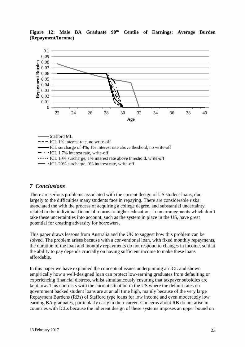
From Figure 12, we see that even this high earning male graduate is protected from having a

RB above 6 percent under an ICL compared to a Stafford ML (where the RB is around 8% in

the first year after graduation). This high earning graduate pays 6% of earnings every year until

the loan is paid back. He pays back two to almost three years faster than under a Stafford ML

depending on which ICL loan scheme is adopted.

0

1000

2000

3000

4000

5000

6000

7000

8000

22 24 26 28 30 32 34 36 38 40

$ p

er y

ear

(2016 p

rice

s)

AgeStafford MLICL 1% interest rate, no write-offICL surcharge of 4%, 1% interest rate above theshold, no write-offICL 1.7% interest rate, write-offICL 10% surcharge, 1% interest rate above threshold, write-offICL 20% surcharge, 0% interest rate, write-off

13 February 2017 23

Figure 12: Male BA Graduate 90th Centile of Earnings: Average Burden

(Repayment/Income)

7 Conclusions

There are serious problems associated with the current design of US student loans, due

largely to the difficulties many students face in repaying. There are considerable risks

associated the with the process of acquiring a college degree, and substantial uncertainty

related to the individual financial returns to higher education. Loan arrangements which don’t

take these uncertainties into account, such as the system in place in the US, have great

potential for creating adversity for borrowers.

This paper draws lessons from Australia and the UK to suggest how this problem can be

solved. The problem arises because with a conventional loan, with fixed monthly repayments,

the duration of the loan and monthly repayments do not respond to changes in income, so that

the ability to pay depends crucially on having sufficient income to make these loans

affordable.

In this paper we have explained the conceptual issues underpinning an ICL and shown

empirically how a well-designed loan can protect low-earning graduates from defaulting or

experiencing financial distress, whilst simultaneously ensuring that taxpayer subsidies are

kept low. This contrasts with the current situation in the US where the default rates on

government backed student loans are at an all time high, mainly because of the very large

Repayment Burdens (RBs) of Stafford type loans for low income and even moderately low

earning BA graduates, particularly early in their career. Concerns about RB do not arise in

countries with ICLs because the inherent design of these systems imposes an upper bound on

0

0.01

0.02

0.03

0.04

0.05

0.06

0.07

0.08

0.09

0.1

22 24 26 28 30 32 34 36 38 40

Rep

ay

men

t B

urd

en

Age

Stafford ML

ICL 1% interest rate, no write-off

ICL surcharge of 4%, 1% interest rate above theshold, no write-off

ICL 1.7% interest rate, write-off

ICL 10% surcharge, 1% interest rate above threshold, write-off

ICL 20% surcharge, 0% interest rate, write-off

13 February 2017 24

RBs and hence avoid repayment problems. ICLs ensure consumption smoothing and provide

insurance against the adverse exigencies that can lead to default.

Using current data, we show that a well-designed ICL system with the characteristics

summarised in Box 1 can overcome virtually all these problems in a simple, efficient,

equitable and cost effective way.

References

Nicholas Barr (1989),‘Alternative Proposals for Student Loans in the United Kingdom’, in

Maureen Woodhall (ed.), Financial Support for Students: Grants, Loans or Graduate

Tax?, Kogan Page, pp. 110-121.

Nicholas Barr (2010), ‘A properly designed ‘graduate contribution’ could work well for UK

students and higher education – even though the original “graduate tax” proposal is a

terrible idea’, LSE British Politics and Policy, 20 August 2010,

http://blogs.lse.ac.uk/politicsandpolicy/a-properly-designed-%E2%80%98graduate-

contribution%E2%80%99-could-work-well-for-uk-students-and-higher-education-even-

though-the-original-%E2%80%98graduate-tax%E2%80%99-proposal-is-a-terrible-idea/

Nicholas Barr (2012a), The Economics of the Welfare State, 5th edition, Oxford and New

York: Oxford University Press.

Nicholas Barr (2012b), ‘The Higher Education White Paper: The good, the bad, the

unspeakable – and the next White Paper’, Social Policy and Administration, Vol. 46, No.

5, October, pp. 483–508.

Bruce Chapman (2014), “Income Contingent Loans: Background” in Bruce Chapman,

Timothy Higgins and Joseph E. Stiglitz (eds), Income Contingent loans: Theory, practice

and prospects, Palgrave McMillan; New York: 11-19.

Bruce Chapman and Lorraine Dearden (2016), “Conceptual and Empirical Issues for

Alternative Student Loan Designs: The Significance of Loan Repayment Burdens for the

US”, forthcoming Annals.

Bruce Chapman, Lorraine Dearden and Louis Hodge (2016), “The distributional and fiscal

implications of different income contingent loan systems for the US”, forthcoming IFS

Working Paper.

Bruce Chapman and Andrew Leigh (2009) “Do Very High Tax Rates Induce Bunching?

Implications for the Design of Income Contingent Loan Schemes”, Economic Record,

Vol. 85 (270) (September): 276-289.

Haroon Chowdry,, Lorraine Dearden, Alissa Goodman and Wenchao Jin. (2012a), The

Distributional Impact of the 2012–13 Higher Education Funding Reforms in England.

Fiscal Studies, 33: 211–236. doi: 10.1111/j.1475-5890.

Haroon Chowdry, Lorraine Dearden, Wenchao Jin and Barnaby Lloyd, November

(2012b), Fees and student support under the new higher education funding regime: what

are different universities doing?, IFS Briefing Notes , BN134,

http://www.ifs.org.uk/bns/bn134.pdf.

Lorraine Dearden, Louis Hodge, Wenchao Jin, Alexander Levine and Laura Williams (2014),

“Financial support for HE students since 2012”, IFS Briefing Notes, BN152,

http://www.ifs.org.uk/bns/bn152.pdf.

13 February 2017 25

Susan Dynarski (2016), “How to – and How Not to – Manage Student Debt”, The Milken

Institute Review, 2nd Quarter.

Milton Friedman (1955). ‘The Role of Government in Education’, in Solo, Robert A. (ed.),

Economics and the Public Interest, New Brunswick, New Jersey: Rutgers University

Press, pp. 123-44.

Johnson, Shane (2016), Bruce Chasing this up.

Adam Looney and Constantine Yannelis (2015). “A crisis in student loans? How changes in

the characteristics of borrowers and in the institutions they attended contributed to rising

loan defaults”. Brookings Papers on Economic Activity Fall, Washington, DC.

Hamish Low, Costas Meghir and Luigi Pistaferri. (2010). "Wage Risk and Employment Risk

over the Life Cycle." American Economic Review, 100(4): 1432-67.

Shapiro, D., Dundar, A., Wakhungu, P.K., Yuan, X., Nathan, A. & Hwang, Y. (2016,

November). Completing College: A National View of Student Attainment Rates – Fall

2010 Cohort (Signature Report No. 12). Herndon, VA: National Student Clearinghouse

Research Center.

Joseph E. Stiglitz (2014), “Remarks on income contingent loans mitigating risk” in Bruce

Chapman, Timothy Higgins and Joseph E. Stiglitz (eds), Income Contingent loans:

Theory, practice and prospects, Palgrave McMillan; New York: 29-37.