getting started modeling processes with solidsprofsite.um.ac.ir/~fanaei/_private/solids 8_4.pdf ·...
TRANSCRIPT
Getting Started Modeling Processes with Solids
Aspen Plus

Version Number: V8.4November 2013
Copyright (c) 1981-2013 by Aspen Technology, Inc. All rights reserved.
Aspen Plus, aspenONE, the aspen leaf logo and Plantelligence and Enterprise Optimization are trademarks orregistered trademarks of Aspen Technology, Inc., Burlington, MA.
All other brand and product names are trademarks or registered trademarks of their respective companies.
This software includes NIST Standard Reference Database 103b: NIST Thermodata Engine Version 7.1
This document is intended as a guide to using AspenTech's software. This documentation contains AspenTech
proprietary and confidential information and may not be disclosed, used, or copied without the prior consent ofAspenTech or as set forth in the applicable license agreement. Users are solely responsible for the proper use ofthe software and the application of the results obtained.
Although AspenTech has tested the software and reviewed the documentation, the sole warranty for the softwaremay be found in the applicable license agreement between AspenTech and the user. ASPENTECH MAKES NOWARRANTY OR REPRESENTATION, EITHER EXPRESSED OR IMPLIED, WITH RESPECT TO THIS DOCUMENTATION,ITS QUALITY, PERFORMANCE, MERCHANTABILITY, OR FITNESS FOR A PARTICULAR PURPOSE.
Aspen Technology, Inc.200 Wheeler RoadBurlington, MA 01803-5501USAPhone: (1) (781) 221-6400Toll Free: (1) (888) 996-7100URL: http://www.aspentech.com

Contents iii
Contents
Who Should Read this Guide ...................................................................................1
Introducing Aspen Plus ...........................................................................................3
Why Use Solids Simulation ................................................................................4
Sessions in this Book ........................................................................................4
Using Backup Files ...........................................................................................4
Related Documentation.....................................................................................5
Technical Support ............................................................................................5
1 Modeling Coal Drying ...........................................................................................7
Coal Drying Flowsheet ......................................................................................7
To Start Aspen Plus ................................................................................8
To Specify the Template for the New Run..................................................8
Specifying Components.....................................................................................9
Defining Properties ......................................................................................... 10
Specifying Nonconventional Solid Physical Property Models.................................. 11
Drawing the Graphical Simulation Flowsheet...................................................... 13
Specifying Title, Stream Properties, and Global Options ...................................... 14
Stream Classes and Substreams ............................................................ 15
To Review the Report Options Specified in the Selected Template ............... 15
Entering Stream Data ..................................................................................... 16
Specifying the Nitrogen Stream.............................................................. 16
Specifying the Wet Coal Feed Stream ..................................................... 17
Specifying Blocks ........................................................................................... 19
Specifying the Flash2 Block ................................................................... 19
Specifying the RStoic Block ................................................................... 19
To Enter the Reaction Stoichiometry ....................................................... 20
Updating the Moisture Content............................................................... 21
Using a Calculator Block to Control Drying......................................................... 21
Creating the H2OIN Variable.................................................................. 22
Creating the Other Variables.................................................................. 23
Calculating the Conversion Variable........................................................ 24
Specifying When the Calculator Block Should Run .................................... 24
Viewing the Calculator Block on the Flowsheet ......................................... 25
Running the Simulation................................................................................... 26
Examining Simulation Results .......................................................................... 26
To View the Stream Results................................................................... 26
To View the Block Results...................................................................... 27
Exiting Aspen Plus .......................................................................................... 28
2 Modeling Coal Combustion .................................................................................29
Coal Combustion Flowsheet ............................................................................. 29
Starting Aspen Plus ........................................................................................ 30
Opening an Existing Run ................................................................................. 30
If You Completed the Simulation in Chapter 1 and Saved the Simulation..... 30

iv Contents
If Your Saved File Solid1.apw is Not Displayed ......................................... 30
To Access the Examples Folder .............................................................. 31
Saving a Run Under a New Name ..................................................................... 31
Modifying the Flowsheet.................................................................................. 31
Changing the Stream Class.............................................................................. 32
To Change the Global Stream Class ........................................................ 32
Adding Components to the Model ..................................................................... 33
Defining Properties ......................................................................................... 34
Change the Heat of Combustion Method for Coal...................................... 35
Specify Methods for Calculating Ash Properties ........................................ 35
Specify the Heat of Combustion for Coal ................................................. 36
Specifying the Air Stream................................................................................ 36
Specifying Unit Operation Models ..................................................................... 37
Specify the RGibbs Reactor Model .......................................................... 37
Specify the RYield Reactor Model............................................................ 39
Specify the Particle Size Distributions ..................................................... 41
Specify the Component Attributes for Ash ............................................... 42
Specify the Splits for the SSplit Block ..................................................... 43
Defining a Calculator Block .............................................................................. 43
Create the Calculator Block ................................................................... 43
Define the Calculator Variables .............................................................. 44
Specify the Calculations to be Performed................................................. 45
Specify When the Calculator Block Should be Run .................................... 45
Running the Simulation................................................................................... 46
Examining Results .......................................................................................... 46
View the Stream Results ....................................................................... 46
View the Block Results .......................................................................... 48
Exiting Aspen Plus .......................................................................................... 49
3 Modeling Gas-Solid Separators...........................................................................51
Gas-Solid Separation Flowsheet ....................................................................... 51
Starting Aspen Plus ........................................................................................ 52
Opening an Existing Run ................................................................................. 52
If You Completed the Simulation in Chapter 2 and Saved the Simulation..... 52
If Your Saved File Solid2.apw is Not Displayed ......................................... 52
To Access the Examples Folder .............................................................. 52
Saving a Run Under a New Name ..................................................................... 53
Modifying the Flowsheet.................................................................................. 53
Changing the Default Particle Size Distribution................................................... 54
To Update the Title for This Simulation ................................................... 54
To Modify the Particle Size Distribution Intervals ...................................... 54
Updating Particle Size Distributions Previously Entered ............................. 55
Specifying the Solids-Handling Blocks ............................................................... 56
To Learn About the Cyclone Model Using Help.......................................... 58
Running the Simulation................................................................................... 59
Examining Results .......................................................................................... 60
To View the Stream Results................................................................... 60
To View the Block Results...................................................................... 61
Exiting Aspen Plus .......................................................................................... 62
4 Modeling Polymer Recovery ...............................................................................63
Polymer Recovery Flowsheet ........................................................................... 63

Contents v
Starting Aspen Plus ........................................................................................ 64
To Specify the Template for the New Run................................................ 64
Specifying Components................................................................................... 65
Defining Properties ......................................................................................... 65
Select a Property Method ...................................................................... 65
Specify Nonconventional Component Property Methods............................. 66
Specify Parameters Used to Calculate POLYMER Properties ........................ 67
Drawing the Flowsheet.................................................................................... 69
To Change the Stream Class for the Simulation........................................ 69
Specifying Title, Stream Properties, and Global Options ...................................... 70
To Review the Report Options Specified in the Selected Template ............... 71
Defining Stream Conditions ............................................................................. 72
Entering Block Specifications ........................................................................... 74
Enter Specifications for the CCD Model.................................................... 74
To Learn More about the Cyclone Model Using Help .................................. 75
Enter Specifications for the Cyclone Model............................................... 76
To Specify That the Mixer Block DRIER Operates at 15 psia ....................... 76
Enter Specifications for the HyCyc Model................................................. 77
Running the Simulation................................................................................... 78
Examining Results .......................................................................................... 79
To View the Stream Results................................................................... 79
To View the Block Results...................................................................... 80
Exiting Aspen Plus .......................................................................................... 83

vi Contents
Who Should Read this Guide 1
Who Should Read this Guide
This guide is suitable for Aspen Plus users who want to model processes
containing solids. Users should be familiar with the procedures covered in
Aspen Plus Getting Started Building and Running a Process Model before
starting these examples.

2 Who Should Read this Guide
Introducing Aspen Plus 3
Introducing Aspen Plus
Aspen Plus can be used to model many processes involving solids. Some of
the solids processing applications that have been modeled with Aspen Plus
include:
Bayer process
Cement kiln
Coal gasification.
Hazardous waste incineration
Iron ore reduction
Zinc smelting/roasting
All of the unit operation models (except Extract) and flowsheeting tools are
available for use in modeling solids processing applications.
This book guides you in introducing solids to a simulation in Aspen Plus. The
four sessions demonstrate the following concepts:
Defining solid components
Changing the global stream class
Defining physical property methods for solid components
Defining component attributes for solid components
Defining a particle size distribution
Modifying the default particle size distribution
Accessing component attributes in a Fortran block
Modifying component attributes in a block
Using solids unit operation models
Getting Started Modeling Processes with Solids assumes that you have an
installed copy of the Aspen Plus software, and that you have done the
sessions in Getting Started Building and Running a Process Model so that you
are familiar with the basics of how to use Aspen Plus.
4 Introducing Aspen Plus
Why Use Solids SimulationThe introduction of solids to a chemical process can affect the process in
many ways. In all cases, the heat and mass balances of the process are
changed, even if the solid essentially passes through the process as an inert
component.
Simulation of the heat and mass balances of a solids process requires physical
property models suitable for solid components. The physical property models
used to characterize a liquid may not be relevant for solids.
In addition to specialized physical property models for solid components,
accurate representation of the solids particle size distribution is required for
some processes. For example, the separation efficiency of a cyclone is highly
dependent on the size of the particles entrained in the feed gas.
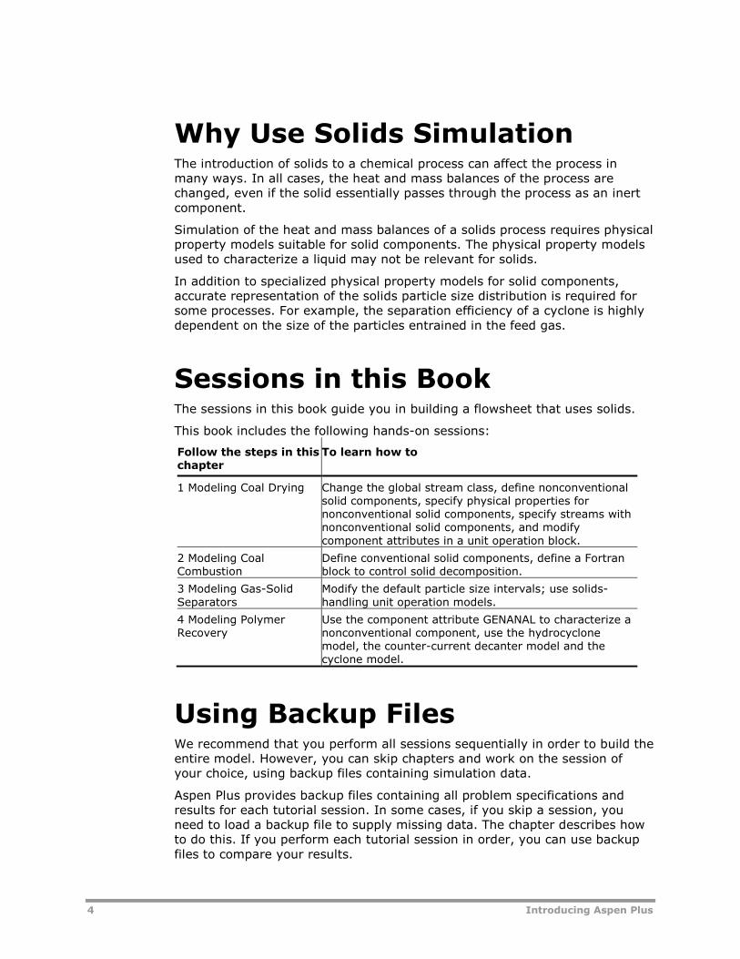
Sessions in this BookThe sessions in this book guide you in building a flowsheet that uses solids.
This book includes the following hands-on sessions:
Follow the steps in this
chapter
To learn how to
1 Modeling Coal Drying Change the global stream class, define nonconventional
solid components, specify physical properties for
nonconventional solid components, specify streams with
nonconventional solid components, and modify
component attributes in a unit operation block.
2 Modeling Coal
Combustion
Define conventional solid components, define a Fortran
block to control solid decomposition.
3 Modeling Gas-Solid
Separators
Modify the default particle size intervals; use solids-
handling unit operation models.
4 Modeling Polymer
Recovery
Use the component attribute GENANAL to characterize a
nonconventional component, use the hydrocyclone
model, the counter-current decanter model and the
cyclone model.
Using Backup FilesWe recommend that you perform all sessions sequentially in order to build the
entire model. However, you can skip chapters and work on the session of
your choice, using backup files containing simulation data.
Aspen Plus provides backup files containing all problem specifications and
results for each tutorial session. In some cases, if you skip a session, you
need to load a backup file to supply missing data. The chapter describes how
to do this. If you perform each tutorial session in order, you can use backup
files to compare your results.
Introducing Aspen Plus 5
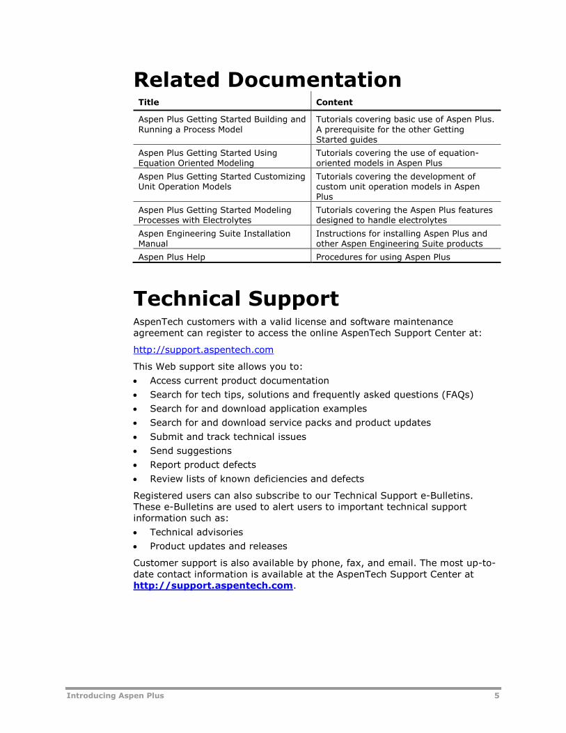
Related DocumentationTitle Content
Aspen Plus Getting Started Building and
Running a Process Model
Tutorials covering basic use of Aspen Plus.
A prerequisite for the other Getting
Started guides
Aspen Plus Getting Started Using
Equation Oriented Modeling
Tutorials covering the use of equation-
oriented models in Aspen Plus
Aspen Plus Getting Started Customizing
Unit Operation Models
Tutorials covering the development of
custom unit operation models in Aspen
Plus
Aspen Plus Getting Started Modeling
Processes with Electrolytes
Tutorials covering the Aspen Plus features
designed to handle electrolytes
Aspen Engineering Suite Installation
Manual
Instructions for installing Aspen Plus and
other Aspen Engineering Suite products
Aspen Plus Help Procedures for using Aspen Plus
Technical SupportAspenTech customers with a valid license and software maintenance
agreement can register to access the online AspenTech Support Center at:
http://support.aspentech.com
This Web support site allows you to:
Access current product documentation
Search for tech tips, solutions and frequently asked questions (FAQs)
Search for and download application examples
Search for and download service packs and product updates
Submit and track technical issues
Send suggestions
Report product defects
Review lists of known deficiencies and defects
Registered users can also subscribe to our Technical Support e-Bulletins.
These e-Bulletins are used to alert users to important technical support
information such as:
Technical advisories
Product updates and releases
Customer support is also available by phone, fax, and email. The most up-to-
date contact information is available at the AspenTech Support Center at
http://support.aspentech.com.

6 Introducing Aspen Plus
1 Modeling Coal Drying 7
1 Modeling Coal Drying
In this simulation you will simulate a coal drying process.
You will:
Define nonconventional solid components.
Specify physical properties for nonconventional solid components.
Change the global stream class.
Specify streams with nonconventional solid components.
Modify component attributes in a unit operation block.
Analyze the results.
Allow about 30 minutes to complete this simulation.
Coal Drying FlowsheetThe process flow diagram and operating conditions for this simulation are
shown in the following figure. A wet coal stream and a nitrogen stream are
fed to a drier. There are two products from the drier: a stream of dried coal
and a stream of moist nitrogen.

8 1 Modeling Coal Drying
To Start Aspen Plus1 From your desktop, click Start and then select Programs.
2 Select AspenTech | Process Modeling <version> | Aspen Plus |
Aspen Plus <version>. The Start Using Aspen Plus window appears
within the Aspen Plus main window.
On this window, Aspen Plus displays links for commands and cases so that
you can quickly enter information or make a selection before proceeding.
In this simulation, start a new case using an Aspen Plus template.
3 Click New on the Start Using Aspen Plus window.
The New dialog box appears. Use this dialog box to specify the template
for the new run. With the template, Aspen Plus automatically sets various
defaults appropriate to your application.
To Specify the Template for the New Run1 Under Installed Templates in the panel on the left side of the New
dialog box, click Solids, then click the Solids with English Units
template.
Information for unit sets, property method, etc. that were pre-defined in
the template is shown on the right side, in the Preview field.
DRIER
Temp = 77 FPres = 14.7 PSICoal Flow = 10000 lb/hrWater Content = 25 wt%
IsobaricAdiabatic
Temp = 270 FPres = 14.7 PSIMass Flow = 50000 lb/hrMole Fraction N2 = 0.999Mole Fraction O2 = 0.001
WET COAL
NITROGEN
EXHAUST
DRY COAL
Water Content = 10 wt%

1 Modeling Coal Drying 9
2 Click Create to apply this template.
It takes a few seconds for Aspen Plus to apply these options.
Specifying ComponentsThe Components - Specifications | Selection sheet is used to enter the
components present in the simulation. The components in this simulation areOH2 , 2N , 2O , and coal.
1 In the first four Component ID fields, enter H2O, N2, O2, and COAL.
Because H2O, N2, and O2 are present in the databanks, WATER,
NITROGEN, and OXYGEN appear in the Component name field. Aspen
Plus does not recognize COAL. Coal is actually a mixture of different
compounds, but for this simulation it will be treated as a single
component.
By default, Aspen Plus assumes all components are of the type
Conventional, indicating that they participate in phase equilibrium
calculations. However, in this simulation, coal will be modeled as a
nonconventional solid.
2 From the COAL Type field, click and select Nonconventional.
The Components - Specifications | Selection sheet is now complete:

10 1 Modeling Coal Drying
3 From the Navigation Pane, select Methods | Specifications.
The Methods - Specifications | Global sheet appears.
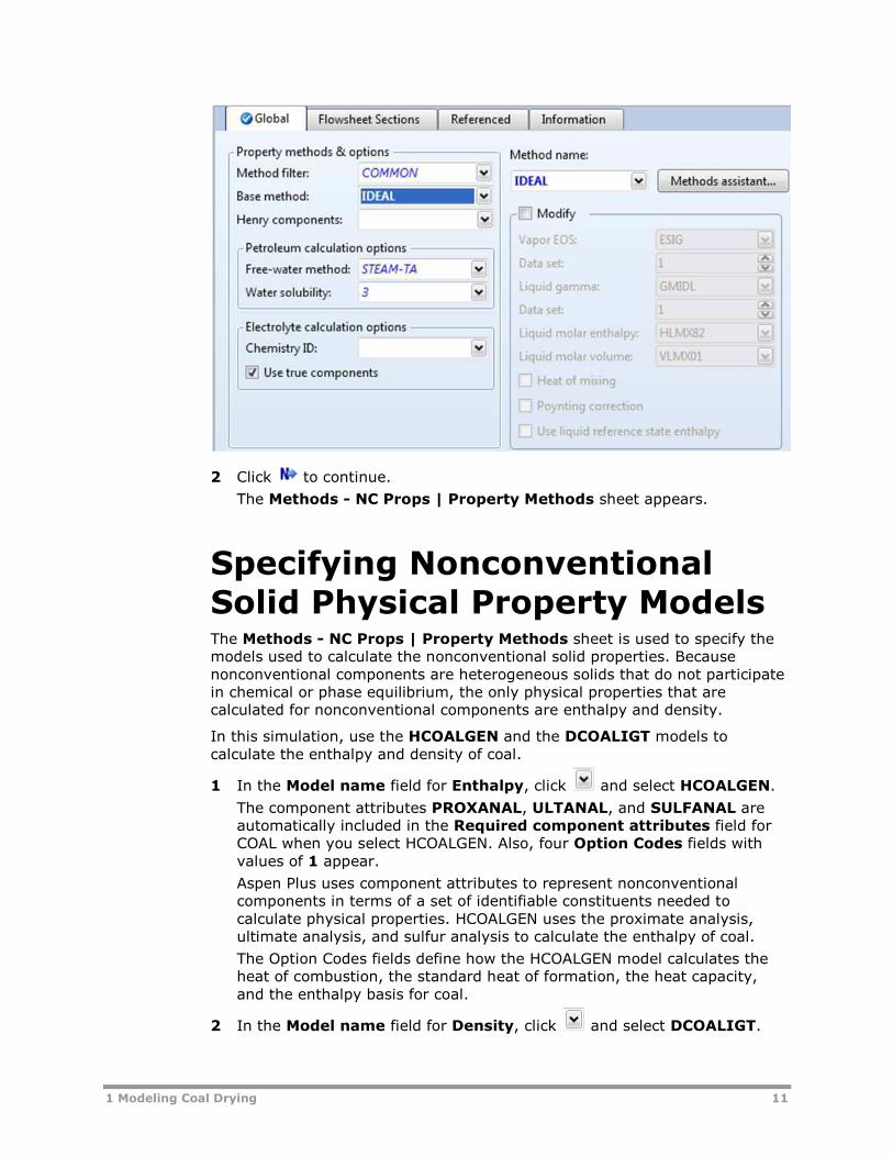
Defining PropertiesThe Methods - Specifications | Global sheet is used to select the
thermodynamic methods used to calculate properties such as K-values,
enthalpy, and density. Property methods in Aspen Plus are categorized into
various process types.
Because the physical property methods for solid components are the same for
all property methods, select a property method based on the conventional
components in the simulation.
The IDEAL property method (Ideal gas and Raoult's Law, as the prompt
indicates) is a good choice for this simulation, since the process involves theconventional components OH2 , 2N , and 2O , at low pressure.
1 In the Base method field, click and select IDEAL.
1 Modeling Coal Drying 11
2 Click to continue.
The Methods - NC Props | Property Methods sheet appears.
Specifying Nonconventional
Solid Physical Property ModelsThe Methods - NC Props | Property Methods sheet is used to specify the
models used to calculate the nonconventional solid properties. Because
nonconventional components are heterogeneous solids that do not participate
in chemical or phase equilibrium, the only physical properties that are
calculated for nonconventional components are enthalpy and density.
In this simulation, use the HCOALGEN and the DCOALIGT models to
calculate the enthalpy and density of coal.
1 In the Model name field for Enthalpy, click and select HCOALGEN.
The component attributes PROXANAL, ULTANAL, and SULFANAL are
automatically included in the Required component attributes field for
COAL when you select HCOALGEN. Also, four Option Codes fields with
values of 1 appear.
Aspen Plus uses component attributes to represent nonconventional
components in terms of a set of identifiable constituents needed to
calculate physical properties. HCOALGEN uses the proximate analysis,
ultimate analysis, and sulfur analysis to calculate the enthalpy of coal.
The Option Codes fields define how the HCOALGEN model calculates the
heat of combustion, the standard heat of formation, the heat capacity,
and the enthalpy basis for coal.
2 In the Model name field for Density, click and select DCOALIGT.
12 1 Modeling Coal Drying
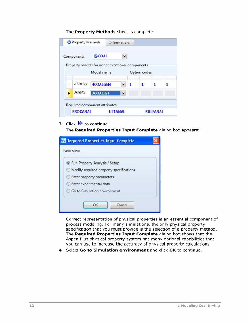
The Property Methods sheet is complete:
3 Click to continue.
The Required Properties Input Complete dialog box appears:
Correct representation of physical properties is an essential component of
process modeling. For many simulations, the only physical property
specification that you must provide is the selection of a property method.
The Required Properties Input Complete dialog box shows that the
Aspen Plus physical property system has many optional capabilities that
you can use to increase the accuracy of physical property calculations.
4 Select Go to Simulation environment and click OK to continue.

1 Modeling Coal Drying 13
Drawing the Graphical
Simulation FlowsheetIn this simulation, begin building the process flowsheet. Since you will enter
your own block and stream IDs, turn off the automatic naming of blocks and
streams, which provide these IDs automatically.
1 From the ribbon, click File. Click Options.
The Options dialog box appears.
2 Select Flowsheet from the panel on the left side of the dialog box.
3 Clear the Automatically assign block name with prefix and
Automatically assign stream name with prefix check boxes under
Stream and unit operation labels.
4 Click Apply and then OK to apply the changes and close the dialog box.
The simulation flowsheet shown in the following figure feeds the WET-
COAL stream and the NITROGEN stream to an RStoic model. In the RStoic
block, a portion of the coal reacts to form water. Because the RStoic
model has a single outlet stream, use a Flash2 model to separate the
dried coal from the moist nitrogen.

14 1 Modeling Coal Drying
5 Place the flowsheet blocks and streams to create the graphical simulation
flowsheet as shown in the figure above. (See Getting Started Building and
Running a Process Model, Chapter 2, if you need to review how to create a
graphical simulation flowsheet.)
6 As you place blocks and streams, Aspen Plus prompts you to enter the
IDs. Enter the block IDs and click OK.
The simulation flowsheet above appears different from the process
diagram in the previous figure because the simulation flowsheet uses two
unit operation models to simulate a single piece of equipment. Also, the
simulation flowsheet defines an extra stream (IN-DRIER) to connect the
two simulation unit operation models. There is no real stream that
corresponds to the simulation stream IN-DRIER.
Specifying Title, Stream
Properties, and Global Options1 From the Navigation Pane, go to Setup | Specifications.
The Setup - Specifications form displays default settings Aspen Plus
uses for other sheets. Use this form to give your simulation a title, and to
review the stream properties and global options that were set when you
selected the Solids with English Units template.
It is always good practice to describe your simulation by entering a title
for the simulation.
2 In the Title field, enter the title Getting Started with Solids –
Simulation 1.
In the Solids with English Units template, the following global defaults
have been set for solids applications:
o ENG units (English Engineering Units)
o Mass Flow Basis for all flow inputs
o MIXCISLD for the global Stream class
3 In the Stream class field, click and select MIXNCPSD.

1 Modeling Coal Drying 15
Stream Classes and Substreams
Stream classes are used to define the structure of simulation streams when
inert solids are present.
The default stream class for most simulations is CONVEN. The CONVEN
stream class has a single substream: the MIXED substream. By definition, all
components in the MIXED substream participate in phase equilibrium
whenever flash calculations are performed.
To introduce inert solid components to a simulation, you must include one or
more additional substreams. Aspen Plus has two other types of substreams
available: the CISOLID substream type and the NC substream type.
The CISOLID substream (Conventional Inert Solid) is used for homogeneous
solids that have a defined molecular weight. The NC substream
(Nonconventional) is used for heterogeneous solids that have no defined
molecular weight. Both the CISOLID substream and the NC substream give
you the option of including a Particle Size Distribution (PSD) for the
substream.
Substreams are combined in different ways to form different stream classes.
The MIXNCPSD stream class contains two substreams: MIXED and NCPSD.
The default stream class of the Solids application type, MIXCISLD, is
insufficient for this simulation since you will use an NC substream with a
particle size distribution for the feed coal. In this simulation, use the
MIXNCPSD stream class.
To Review the Report Options Specified in
the Selected Template4 From the Navigation Pane, click the Setup | Report Options form.
5 Click the Stream tab.
16 1 Modeling Coal Drying
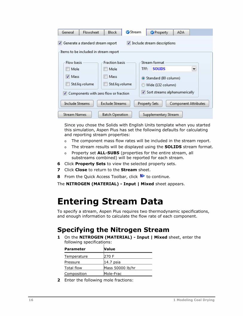
Since you chose the Solids with English Units template when you started
this simulation, Aspen Plus has set the following defaults for calculating
and reporting stream properties:
o The component mass flow rates will be included in the stream report.
o The stream results will be displayed using the SOLIDS stream format.
o Property set ALL-SUBS (properties for the entire stream, all
substreams combined) will be reported for each stream.
6 Click Property Sets to view the selected property sets.
7 Click Close to return to the Stream sheet.
8 From the Quick Access Toolbar, click to continue.
The NITROGEN (MATERIAL) - Input | Mixed sheet appears.
Entering Stream DataTo specify a stream, Aspen Plus requires two thermodynamic specifications,
and enough information to calculate the flow rate of each component.
Specifying the Nitrogen Stream1 On the NITROGEN (MATERIAL) - Input | Mixed sheet, enter the
following specifications:
Parameter Value
Temperature 270 F
Pressure 14.7 psia
Total flow Mass 50000 lb/hr
Composition Mole-Frac
2 Enter the following mole fractions:

1 Modeling Coal Drying 17
Component Value
N2 0.999
O2 0.001
3 Click to continue.
Specifying the Wet Coal Feed Stream
The WET-COAL (MATERIAL) - Input | Mixed sheet appears. Substream
MIXED appears by default. To access the NCPSD substream:
4 Click the tab NC Solid. In the Substream name field, verify NCPSD has
been selected.
5 For the NCPSD substream, enter the following specifications:
Parameter Value
Temperature 77 F
Pressure 14.7 psia
COAL Mass flow 10000 lb/hr
6 Click Particle Size Distribution to display the PSD parameters.
By default, Aspen Plus uses a particle size distribution of 10 size ranges
covering 20 microns each. The default size ranges are appropriate for this
simulation. On this sheet, enter the weight fraction of coal in each size
range.
7 On the last four Weight fraction fields, enter the following values:
Interval Weight fraction
7 0.1
8 0.2
9 0.3
10 0.4

18 1 Modeling Coal Drying
8 Click Component Attribute.
In this section, enter the component attributes for the component COAL in
the NCPSD substream. The values in PROXANAL, ULTANAL, and SULFANAL
are defined as weight % on a dry basis, except for Moisture in PROXANAL.
9 Enter the component attribute values for coal. For the attribute
PROXANAL, enter these values:
Element Value
Moisture 25
FC 45.1
VM 45.7
Ash 9.2
10 In the Attribute ID field, click and select ULTANAL.
11 For the attribute ULTANAL, enter these values:
Element Value
Ash 9.2
Carbon 67.1
Hydrogen 4.8
Nitrogen 1.1
Chlorine 0.1
Sulfur 1.3
Oxygen 16.4

1 Modeling Coal Drying 19
12 In the Attribute ID field, click and select SULFANAL.
13 For the attribute SULFANAL, enter these values:
Element Value
Pyritic 0.6
Sulfate 0.1
Organic 0.6
The values meet the following consistency requirements:
o SULFANAL values sum to the ULTANAL value for sulfur.
o ULTANAL value for ash equals the PROXANAL value for ash.
o ULTANAL values sum to 100.
o PROXANAL values for FC, VM, and ASH sum to 100.
14 Click to continue.
The DRY-FLSH (Flash2) - Input | Specifications sheet appears.
Specifying BlocksThe unit operation models RStoic and Flash2 simulate a single piece of plant
equipment for drying coal. Nitrogen provides the heat for coal drying. Both
the RStoic and Flash2 models are isobaric and adiabatic.
Specifying the Flash2 Block
On the DRY-FLSH (Flash2) - Input | Specifications sheet:
1 In the Flash Type fields, where Temperature is selected, click and
change it to Duty.
2 In the Pressure field, enter 14.7 psia.
3 In the Duty field, enter 0 Btu/hr.
4 Click to continue.
Specifying the RStoic Block
The DRY-REAC (RStoic) - Setup | Specifications sheet appears.
1 In the Pressure field, enter 14.7 psia.
2 In the Flash Type fields, where Temperature is selected, click and
change it to Duty.
3 In the Heat duty field, enter 0 Btu/hr.
4 Click to continue.
The DRY-REAC (RStoic) - Setup | Reactions sheet appears.
This RStoic block models the drying of coal. Although coal drying is not
normally considered a chemical reaction, you are using an RStoic block to
convert a portion of the coal to form water. The following equation is the
chemical reaction for coal drying:

20 1 Modeling Coal Drying
OH0555084.0COAL(wet) 2
Aspen Plus treats all nonconventional components as if they have a
molecular weight of 1.0. The reaction indicates that 1 mole (or 1 lb.) of
coal reacts to form 0.0555084 mole (or 1 lb.) of water.
To Enter the Reaction Stoichiometry1 Click New.
The Edit Stoichiometry dialog box appears. A reaction number of 1 is
automatically chosen.
2 In the Reactants | Component field, click and select COAL.
3 In the Reactants | Coefficient field, enter 1.
Note that the stoichiometric coefficient for reactants is displayed as
negative, -1.
4 In the Products | Component field, click and select H2O.
5 In the Products | Coefficient field, enter 0.0555084.
The conversion for this reaction must be set to achieve the proper amount
of drying.
6 Select the Fractional conversion option.
7 In the Products generation section, for the Fractional conversion
field, enter 0.2; in the of component field, click and select COAL.
The fraction conversion of Coal of 0.2 is a temporary value that you will
override later with a Calculator block.
1 Modeling Coal Drying 21
8 Click Close to return to the DRY-REAC (RStoic) - Setup | Reactions
sheet.
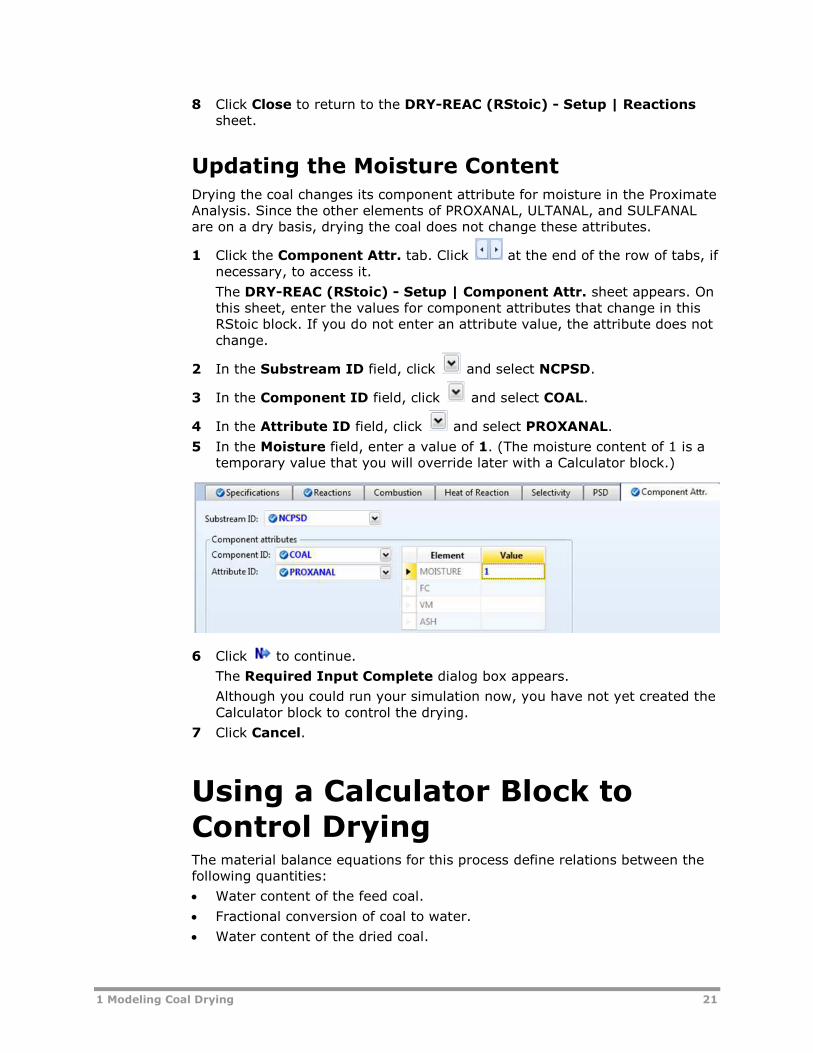
Updating the Moisture Content
Drying the coal changes its component attribute for moisture in the Proximate
Analysis. Since the other elements of PROXANAL, ULTANAL, and SULFANAL
are on a dry basis, drying the coal does not change these attributes.
1 Click the Component Attr. tab. Click at the end of the row of tabs, if
necessary, to access it.
The DRY-REAC (RStoic) - Setup | Component Attr. sheet appears. On
this sheet, enter the values for component attributes that change in this
RStoic block. If you do not enter an attribute value, the attribute does not
change.
2 In the Substream ID field, click and select NCPSD.
3 In the Component ID field, click and select COAL.
4 In the Attribute ID field, click and select PROXANAL.
5 In the Moisture field, enter a value of 1. (The moisture content of 1 is a
temporary value that you will override later with a Calculator block.)
6 Click to continue.
The Required Input Complete dialog box appears.
Although you could run your simulation now, you have not yet created the
Calculator block to control the drying.
7 Click Cancel.
Using a Calculator Block to
Control DryingThe material balance equations for this process define relations between the
following quantities:
Water content of the feed coal.
Fractional conversion of coal to water.
Water content of the dried coal.
22 1 Modeling Coal Drying
100 100
H 2OIN H 2OOUTCOALIN COALOUT COALIN CONV (1)
COALIN COALOUT COALIN CONV (2)
Where:
COALIN = Mass flow rate of coal in stream WET-COAL
COALOUT = Mass flow rate of coal in stream IN-DRIER
H2OIN = Percent moisture in the coal in stream WET-COAL
H2ODRY = Percent moisture in the coal in stream IN-DRIER
CONV = Fractional conversion of coal to H2O in the block
DRY-REAC
Equation 1 is the material balance for water, and equation 2 is the overall
material balance. These equations can be combined to yield equation 3:
( )
(100 )
H 2OIN H 2OOUTCONV
H 2OOUT
(3)
Use equation 3 in a Calculator block to ensure these three specifications are
consistent.
The Calculator block specifies the moisture content of the dried coal and
calculates the corresponding conversion of coal to water.
Using a Calculator block to set specifications allows you to run different cases
easily.
1 From the Navigation Pane, select Flowsheeting Options | Calculator.
The Calculator object manager appears.
2 Click New to create a new Calculator block.
The Create New ID dialog box appears, displaying an automatically
generated Calculator ID, C-1.
3 Delete the ID C-1 and enter the ID WATER and click OK.
The WATER | Define sheet appears.
4 Ensure that the Active checkbox is checked.
Use this sheet to access the flowsheet variables you want to use in the
Calculator block. Define the three Calculator variables from equation 3:
H2OIN, H2ODRY, and CONV.
H2OIN is the water content of the feed coal. The H2OIN variable accesses the
first element (percent moisture) of the component attribute PROXANAL for
component COAL in the NCPSD substream of stream WET-COAL.
Creating the H2OIN Variable1 Click New.
The Create new variable dialog box appears.
2 In the Variable name field, enter H2OIN and click OK.
3 Click H2OIN in the grid. It appears in the Edit selected variable
section.

1 Modeling Coal Drying 23
4 In the Category frame, click Streams.
5 In the Reference frame, in the Type field, click and select
Compattr-Var since the variable is a component attribute.
When you are specifying variables, Aspen Plus displays the other fields
necessary to complete the variable definition. In this case, the Stream
field appears.
6 In the Stream field, click and select WET-COAL.
The Substream and Component fields appear. In this example, do not
modify the default choice of NCPSD in the Substream field.
7 In the Component field, click and select COAL.
The Attribute field appears.
8 In the Attribute field, click and select PROXANAL.
9 In the Element field, enter 1. Press Enter.
The blue check mark next to H2OIN in the Variable name field indicates
that the definition of variable H2OIN is complete:
Creating the Other Variables
CONV and H2ODRY are block variables in the DRY-REAC block. CONV is the
fractional conversion of the first (and only) reaction. H2ODRY is the moisture
content of the coal leaving the RStoic block.
1 Click New to create another variable, CONV. Create the new CONV and
H2ODRY variables as shown:
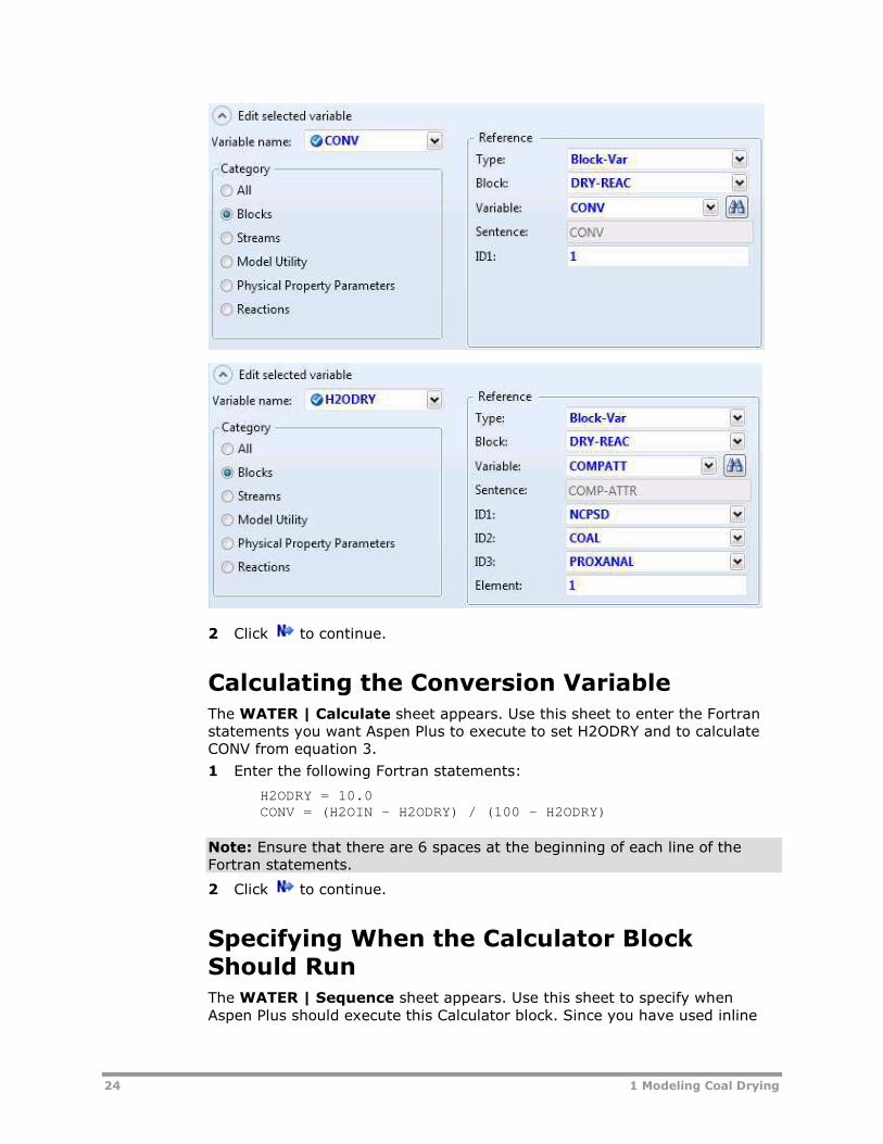
24 1 Modeling Coal Drying
2 Click to continue.
Calculating the Conversion Variable
The WATER | Calculate sheet appears. Use this sheet to enter the Fortran
statements you want Aspen Plus to execute to set H2ODRY and to calculate
CONV from equation 3.
1 Enter the following Fortran statements:
H2ODRY = 10.0
CONV = (H2OIN - H2ODRY) / (100 - H2ODRY)
Note: Ensure that there are 6 spaces at the beginning of each line of the
Fortran statements.
2 Click to continue.
Specifying When the Calculator Block
Should Run
The WATER | Sequence sheet appears. Use this sheet to specify when
Aspen Plus should execute this Calculator block. Since you have used inline

1 Modeling Coal Drying 25
Fortran to modify the specifications for the RStoic block DRY-REAC, this
Calculator block should execute immediately prior to DRY-REAC.
1 In the Execute field, click and select Before.
2 In the Block type field, click and select Unit operation.
3 In the Block name field, click and select DRY-REAC.
4 Click to continue.
The Required Input Complete dialog box appears.
5 Click Cancel.
Viewing the Calculator Block on the
Flowsheet
Go to the Flowsheet to verify that the Calculator block WATER has been
placed. If it does not appear, on the Flowsheet | Modify tab of the ribbon,
click Display Options and click the Calculators and Calculator
Connections options to make sure that check marks appear in front of these
items.
The Flowsheet with the Calculator block added looks like this:
The connections between the WATER block and the block DRY-REAC and
stream WET-COAL appear as red dashed lines.
26 1 Modeling Coal Drying
Running the Simulation1 Click and click OK to run the simulation.
The Control Panel window appears, allowing you to monitor and interact
with the Aspen Plus simulation calculations.
As Aspen Plus performs the analysis, status messages display in the
Control Panel.
The simulation completes without warnings or errors.
When the calculations finish, the message Results Available appears in the
status area at the bottom left of the main window.
2 Examine the results of your simulation.
Examining Simulation Results
To View the Stream Results1 In the Control Panel, click Check Status.
The Results Summary - Run Status | Status sheet appears, indicating
that the simulation completed normally.
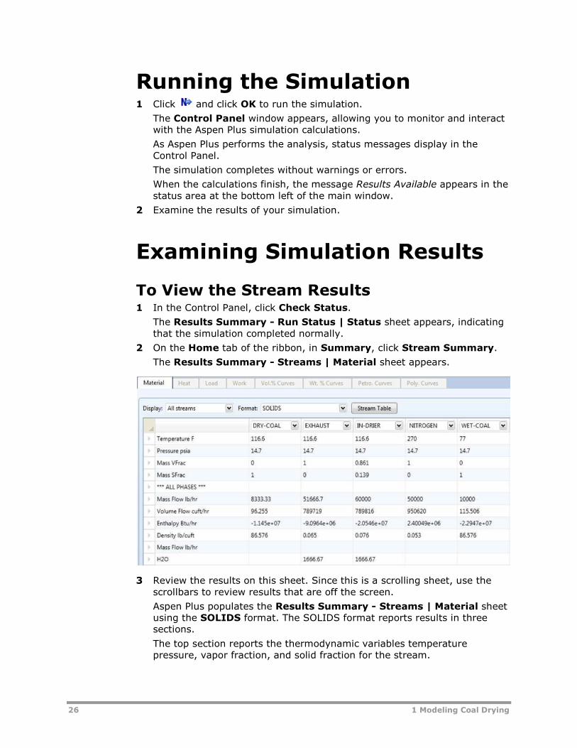
2 On the Home tab of the ribbon, in Summary, click Stream Summary.
The Results Summary - Streams | Material sheet appears.
3 Review the results on this sheet. Since this is a scrolling sheet, use the
scrollbars to review results that are off the screen.
Aspen Plus populates the Results Summary - Streams | Material sheet
using the SOLIDS format. The SOLIDS format reports results in three
sections.
The top section reports the thermodynamic variables temperature
pressure, vapor fraction, and solid fraction for the stream.
1 Modeling Coal Drying 27
The second section, beginning with ***ALL PHASES***, reports properties
and component mass flow rates summed over all substreams.
Examination of the component mass flow rates indicates that 1667 lb/hr
of H2O are removed from the coal by the drying process.
The third section, beginning with *** SUBSTREAM NCPSD ***, displays
information that is appropriate only for the NCPSD substream. In this
case, it displays the component attributes for coal, and the overall particle
size distribution for the NCPSD substream. Note that the moisture in the
PROXANAL is different for stream DRY-COAL and stream WET-COAL.
Stream summary results can also be displayed one substream at a time,
by using the FULL format.
4 In the Format field, click and select FULL.
5 Examine the results reported for the MIXED and NCPSD substreams.
When you are done, return to the SOLIDS Format.
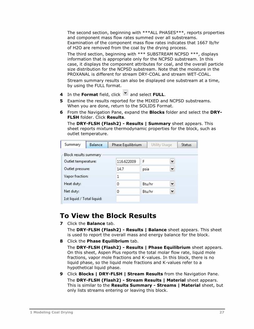
6 From the Navigation Pane, expand the Blocks folder and select the DRY-
FLSH folder. Click Results.
The DRY-FLSH (Flash2) - Results | Summary sheet appears. This
sheet reports mixture thermodynamic properties for the block, such as
outlet temperature.
To View the Block Results7 Click the Balance tab.
The DRY-FLSH (Flash2) - Results | Balance sheet appears. This sheet
is used to report the overall mass and energy balance for the block.
8 Click the Phase Equilibrium tab.
The DRY-FLSH (Flash2) - Results | Phase Equilibrium sheet appears.
On this sheet, Aspen Plus reports the total molar flow rate, liquid mole
fractions, vapor mole fractions and K-values. In this block, there is no
liquid phase, so the liquid mole fractions and K-values refer to a
hypothetical liquid phase.
9 Click Blocks | DRY-FLSH | Stream Results from the Navigation Pane.
The DRY-FLSH (Flash2) - Stream Results | Material sheet appears.
This is similar to the Results Summary - Streams | Material sheet, but
only lists streams entering or leaving this block.

28 1 Modeling Coal Drying
10 Click Blocks | DRY-REAC | Results to move to the DRY-REAC (RStoic)
- Results | Summary sheet.
This sheet, like the DRY-FLSH (Flash2) - Results | Summary sheet,
displays the mixture thermodynamic results for the block, such as
temperature.
11 Click the Balance tab to move to the next sheet with results.
The DRY-REAC (RStoic) - Results | Balance sheet appears. This sheet
displays the mass and energy balance for the block. Because this block
contains a reaction between the NCPSD substream and the MIXED
substream, neither the conventional components nor the nonconventional
are in mass balance. The total mass balance for the stream shows a very
small relative difference.
12 Click the Phase Equilibrium tab to move to the next sheet with results.
The DRY-REAC (RStoic) - Results | Phase Equilibrium sheet appears.
This sheet serves the same function as the DRY-FLSH (Flash2) -
Results | Phase Equilibrium sheet.
Exiting Aspen PlusWhen you are finished working with this model, save your simulation and exit
Aspen Plus as follows:
1 From the ribbon, select File | Save as | Aspen Plus Document.
The Save as dialog box appears.
2 In the File name field, enter Solid1.
3 Click Save.
Aspen Plus saves the simulation as the Aspen Plus Document file,
Solid1.apw, in your default working directory (displayed in the Save in
field).
4 From the ribbon, select File | Exit.
Note: The chapter 2 simulation uses this run as the starting point.

2 Modeling Coal Combustion 29
2 Modeling Coal Combustion
In this simulation, you will simulate a coal combustion process.
You will:
Start with the simulation you created in chapter 1.
Modify the flowsheet.
Change the stream class.
Add the components needed for combustion.
Specify the unit operation models.
Define a Fortran block to control the decomposition of coal.
Analyze the results.
Allow about 45 minutes to complete this simulation.
Coal Combustion FlowsheetThe process flow diagram, operating conditions and problem definition for this
simulation are shown in the following figure. The feed to the furnace is the
dried coal stream from chapter 1. After combustion, the ash is separated from
the gaseous combustion products.

30 2 Modeling Coal Combustion
DRIER
Temp = 77 FPres = 14.7 PSICoal Flow = 10000 lb/hrWater Content = 25 wt%
IsobaricAdiabatic
Temp = 270 FPres = 14.7 PSIMass Flow = 50000 lb/hrMole Fraction N2 = 0.999Mole Fraction O2 = 0.001
WET COAL
NITROGEN
EXHAUST
DRY COAL
Water Content = 10 wt%
BURN
RGIBBS
PRODUCTS
AIR
SEPARATE
SSPLIT
GASES
SOLIDS
Perfectseparation
Temp = 77 FPres = 14.7 PSIMass Flow = 90000 lb/hrMole Fraction N2 = 0.79Mole Fraction O2 = 0.21
IsobaricAdiabatic
Starting Aspen Plus1 From your desktop, select Start and then select Programs.
2 Select AspenTech | Process Modeling <version> | Aspen Plus |
Aspen Plus <version>.
Opening an Existing Run
If You Completed the Simulation in Chapter
1 and Saved the Simulation
On the Start Using Aspen Plus window, click Solid1.apw in Recent
Models.
If Your Saved File Solid1.apw is Not
Displayed1 Click Open.
The Open dialog box appears.
2 Navigate to the directory that contains your saved file Solid1.apw.
3 Select Solid1.apw in the list of files and click Open.
Note: If you did not create the simulation in chapter 1, open the backup file
solid1.bkp from the Examples folder.

2 Modeling Coal Combustion 31
To Access the Examples Folder1 Click Open File.
The Open dialog box appears.
2 At the left, under Favorites, click Aspen Plus <version> Examples.
By default, this folder contains folders that are provided with Aspen Plus.
3 Double-click the Examples folder, then the GSG_Solids folder.
4 Select Solid1.bkp and click Open.
Saving a Run Under a New
NameBefore creating a new run, create and save a copy of Solid1 with a new Run
ID, Solid2. Then you can make modifications under this new Run ID.
1 From the ribbon, select File | Save As | Aspen Plus Document.
2 In the Save As dialog box, choose the directory where you want to save
the simulation.
3 In the File name field, enter Solid2.
4 Click Save to save the simulation and continue.
Aspen Plus creates a new simulation model, Solid2, which is a copy of the
base case simulation, Solid1.
Modifying the FlowsheetUse the RGibbs model to simulate combustion of the dry coal. RGibbs models
chemical equilibrium by minimizing Gibbs free energy. However, the Gibbs
free energy of coal cannot be calculated because it is a nonconventional
component.
Before feeding the dried coal to the RGibbs block, decompose the coal into its
constituent elements. This is done in the RYield block, DECOMP. The heat of
reaction associated with the decomposition of coal must be considered in the
coal combustion. Use a heat stream to carry this heat of reaction from the
RYield block to the RGibbs block.
Finally, separate the combustion gases from the ash using the Aspen Plus
model SSplit for this separation.
Modify the flowsheet to include the additional unit operation models and
streams, as shown below. (See Getting Started Building and Running a
Process Model, Chapter 2, if you need to review how to create a graphical
simulation flowsheet.) You will add three unit operation models (an RYield, an
RGibbs, and an SSplit), a calculator block (its connections, shown in red, will
be created in the steps that follow), five material streams, and one heat
stream.

32 2 Modeling Coal Combustion
The simulation flowsheet appears different from the process diagram in the
previous figure because the simulation flowsheet uses two unit operation
models to simulate a single piece of equipment. An extra stream (INBURNER)
is defined to connect the two simulation unit operation models. There is no
real stream that corresponds with the simulation stream INBURNER.
Changing the Stream ClassBecause the decomposition of coal forms carbon, you must use a stream class
that includes conventional solids. Use the MCINCPSD stream class.
MCINCPSD contains the following substreams:
MIXED
CIPSD
NCPSD
To Change the Global Stream Class1 From the Navigation Pane, go to Setup | Specifications.
The Setup - Specifications | Global sheet appears.
2 In the Stream class field, click and select MCINCPSD.
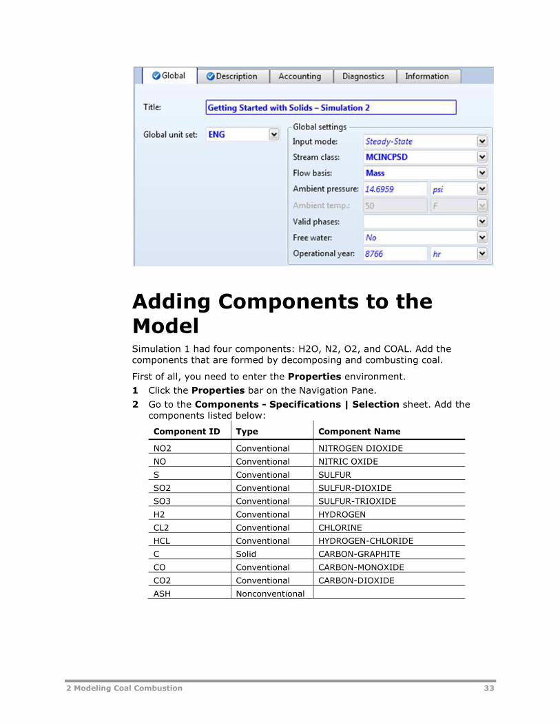
3 In the Title field, enter Getting Started with Solids – Simulation 2.
2 Modeling Coal Combustion 33
Adding Components to the
ModelSimulation 1 had four components: H2O, N2, O2, and COAL. Add the
components that are formed by decomposing and combusting coal.
First of all, you need to enter the Properties environment.
1 Click the Properties bar on the Navigation Pane.
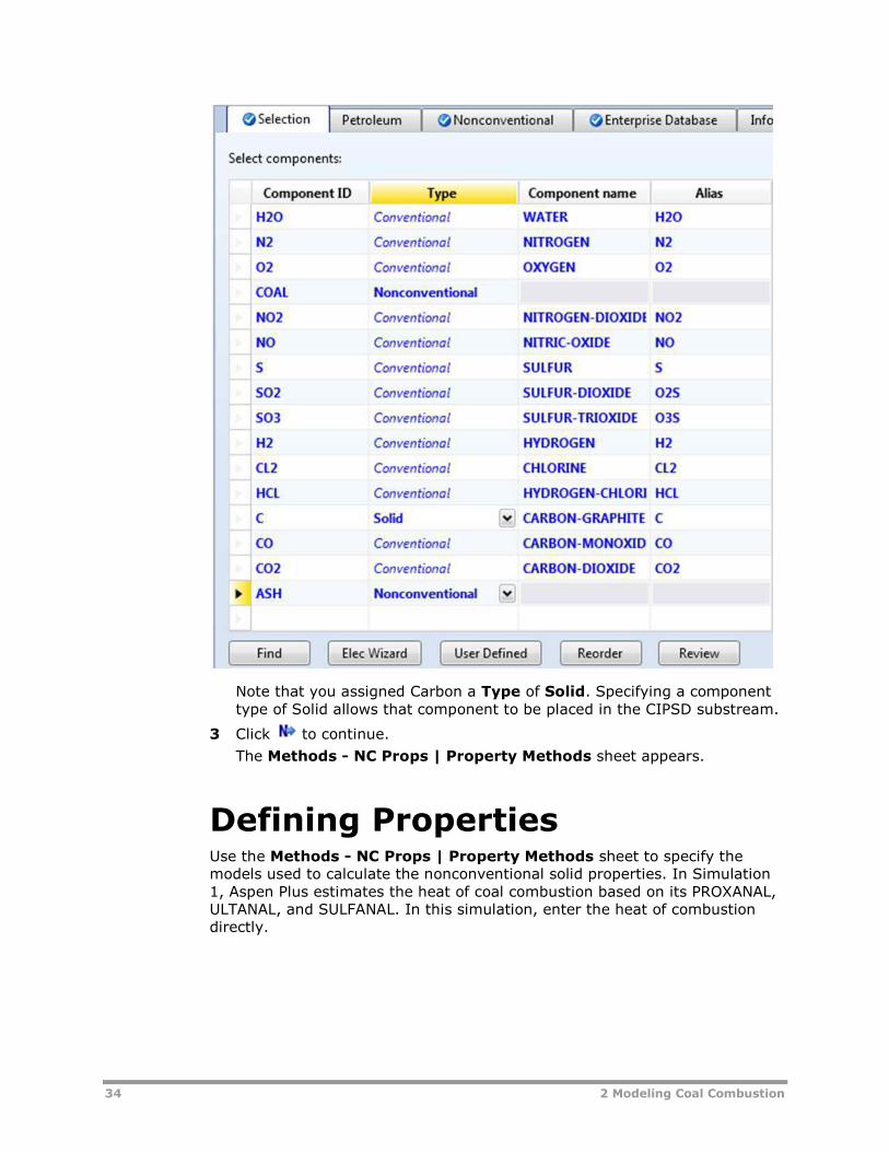
2 Go to the Components - Specifications | Selection sheet. Add the
components listed below:
Component ID Type Component Name
NO2 Conventional NITROGEN DIOXIDE
NO Conventional NITRIC OXIDE
S Conventional SULFUR
SO2 Conventional SULFUR-DIOXIDE
SO3 Conventional SULFUR-TRIOXIDE
H2 Conventional HYDROGEN
CL2 Conventional CHLORINE
HCL Conventional HYDROGEN-CHLORIDE
C Solid CARBON-GRAPHITE
CO Conventional CARBON-MONOXIDE
CO2 Conventional CARBON-DIOXIDE
ASH Nonconventional
34 2 Modeling Coal Combustion
Note that you assigned Carbon a Type of Solid. Specifying a component
type of Solid allows that component to be placed in the CIPSD substream.
3 Click to continue.
The Methods - NC Props | Property Methods sheet appears.
Defining PropertiesUse the Methods - NC Props | Property Methods sheet to specify the
models used to calculate the nonconventional solid properties. In Simulation
1, Aspen Plus estimates the heat of coal combustion based on its PROXANAL,
ULTANAL, and SULFANAL. In this simulation, enter the heat of combustion
directly.

2 Modeling Coal Combustion 35
Change the Heat of Combustion Method for
Coal
1 In the Component field, click and select COAL.
2 Change the first HCOALGEN Option codes field from 1 to 6.
Specify Methods for Calculating Ash
Properties
You must also specify how Aspen Plus calculates the enthalpy and density of
ASH.
1 In the Component field, click and select ASH.
2 In the Model name field for Enthalpy, click and select HCOALGEN.
The Option codes defaults of 1, 1, 1, and 1 are acceptable for ASH.
3 In the Model name field for Density, click and select DCOALIGT.

36 2 Modeling Coal Combustion
Specify the Heat of Combustion for Coal
You just specified that Aspen Plus will use a user-specified value for the heat
of combustion of coal. Now you must specify that value.
1 From the Navigation Pane, select Methods | Parameters | Pure
Components.
The Pure Components object manager appears.
2 Click New.
The New Pure Component Parameters dialog box appears. The heat of
combustion for coal is a Nonconventional type.
3 Select the Nonconventional option.
4 Delete the default name NC-1 and enter HEAT as the new name in the
Enter new name or accept default field.
5 Click OK.
The Pure Components - HEAT | Input sheet appears.
6 In the Parameter field, click and select HCOMB.
Note that HCOMB is the heat of combustion on a dry basis. Use the
following equation to convert the heat of combustion on a wet basis to a
dry basis:
Moisture%100
100*(wet)CombustionofHeatHCOMB
7 In the first line under the Nonconventional component parameter
column, click and select COAL.
8 In the parameter value field directly below COAL, enter the heat of
combustion on a dry basis: 11700 Btu/lb.
9 Click to continue.
The Properties Input Complete dialog box appears.
10 Select Go to Simulation environment and click OK to access the next
required input sheet in the Simulation Environment.
Specifying the Air StreamClick Streams | AIR | Input from the Navigation Pane. The AIR
(MATERIAL) - Input | Mixed sheet appears. Aspen Plus requires two

2 Modeling Coal Combustion 37
thermodynamic specifications, and enough information to calculate the flow
rate of each component.
1 Enter the following thermodynamic specifications for the MIXED
substream:
Parameter Value
Temperature 77 F
Pressure 14.7 psia
2 In the Composition field, click and select Mole-Frac.
3 Enter the following mole fractions:
Component Value
N2 0.79
O2 0.21
4 Enter a total mass flow of 90000 lb/hr.
5 Click to continue.
Specifying Unit Operation
ModelsThe BURN (RGibbs) - Setup | Specifications sheet appears.
RGibbs is used to model reactions that come to chemical equilibrium. RGibbs
calculates chemical equilibrium and phase equilibrium by minimizing the
Gibbs free energy of the system. Therefore, you do not need to specify the
reaction stoichiometry.
Specify the RGibbs Reactor Model
On the BURN (RGibbs) - Setup | Specifications sheet, enter your
thermodynamic specifications. This reactor will be at atmospheric pressure.
1 In the Pressure field, enter 14.7 psia.

38 2 Modeling Coal Combustion
The heat duty for this reactor is specified by the heat stream Q-DECOMP.
2 In the Calculation options field, verify that Calculate phase
equilibrium and chemical equilibrium has been selected.
3 Click the Products tab.
The BURN (RGibbs) - Setup | Products sheet appears. On this sheet,
enter the list of products that may exist at equilibrium.
By default, RGibbs assumes that all of the components that are listed on
the Components - Specifications | Selection sheet are potential
products in the vapor phase or the liquid phase. This default is not
appropriate for this simulation, since any carbon that remains after
combustion would be solid.
4 Select Identify possible products.
The Products list appears. For this simulation, all components are
potential MIXED substream products, except for carbon, which is a solid
product. Carbon must be assigned a phase of Pure Solid. This means that
any carbon that forms will be present as a pure, solid phase, not present
as a solid solution or alloy.
5 In the products list, enter the component species and phases shown
below: (Be sure to change the Phase for C to PureSolid.)
Component Phase Component Phase
H2O Mixed SO3 Mixed
N2 Mixed H2 Mixed
O2 Mixed CL2 Mixed
NO2 Mixed HCL Mixed
NO Mixed C PureSolid
S Mixed CO Mixed
SO2 Mixed CO2 Mixed

2 Modeling Coal Combustion 39
6 Click to continue.
Specify the RYield Reactor Model
The DECOMP (RYield) - Setup | Specifications sheet appears. RYield is
used to simulate a reactor with a known yield, and does not require reaction
stoichiometry and kinetics.
1 On the DECOMP (RYield) - Setup | Specifications sheet, enter the
pressure and temperature:
Parameter Value
Pressure 14.7 psia
Temperature 77 F

40 2 Modeling Coal Combustion
2 Click to continue.
The Yield sheet appears.
For this simulation, the yield distribution you enter on this sheet is not the
true yield distribution. Use a Calculator block to calculate the actual yield
distribution from the component attributes for coal in the feed stream to
the RYield model (stream DRY-COAL).
3 Enter the component yields as follows:
Component Basis Yield
H2O Mass 0.2
ASH Mass 0.2
C (CIPSD) Mass 0.1
H2 Mass 0.1
N2 Mass 0.1
CL2 Mass 0.1
S Mass 0.1
O2 Mass 0.1

2 Modeling Coal Combustion 41
In addition to the MIXED substream products, this RYield block forms
carbon in the CIPSD substream and ash in the NCPSD substream. To fully
specify the yield, specify the particle size distributions of the CIPSD and
NCPSD substream and the component attributes of the ash that is formed.
Specify the Particle Size Distributions1 Click the PSD tab.
The DECOMP (RYield) - Setup | PSD sheet appears.
2 In the Substream ID field, click and select CIPSD.
3 Specify the weight fractions for the last four intervals of the particle size
distribution for the carbon formed in the CIPSD substream:
Interval Weight Fraction
7 0.1
8 0.2
9 0.3
10 0.4
It is not necessary to enter zero for intervals 1 through 6.
You must also define the particle size distribution for the NCPSD
substream.
4 In the Substream ID field, click and select NCPSD.
5 Enter the same weight fractions for the particle size distribution for the
NCPSD substream that you entered for the CIPSD substream above.
42 2 Modeling Coal Combustion
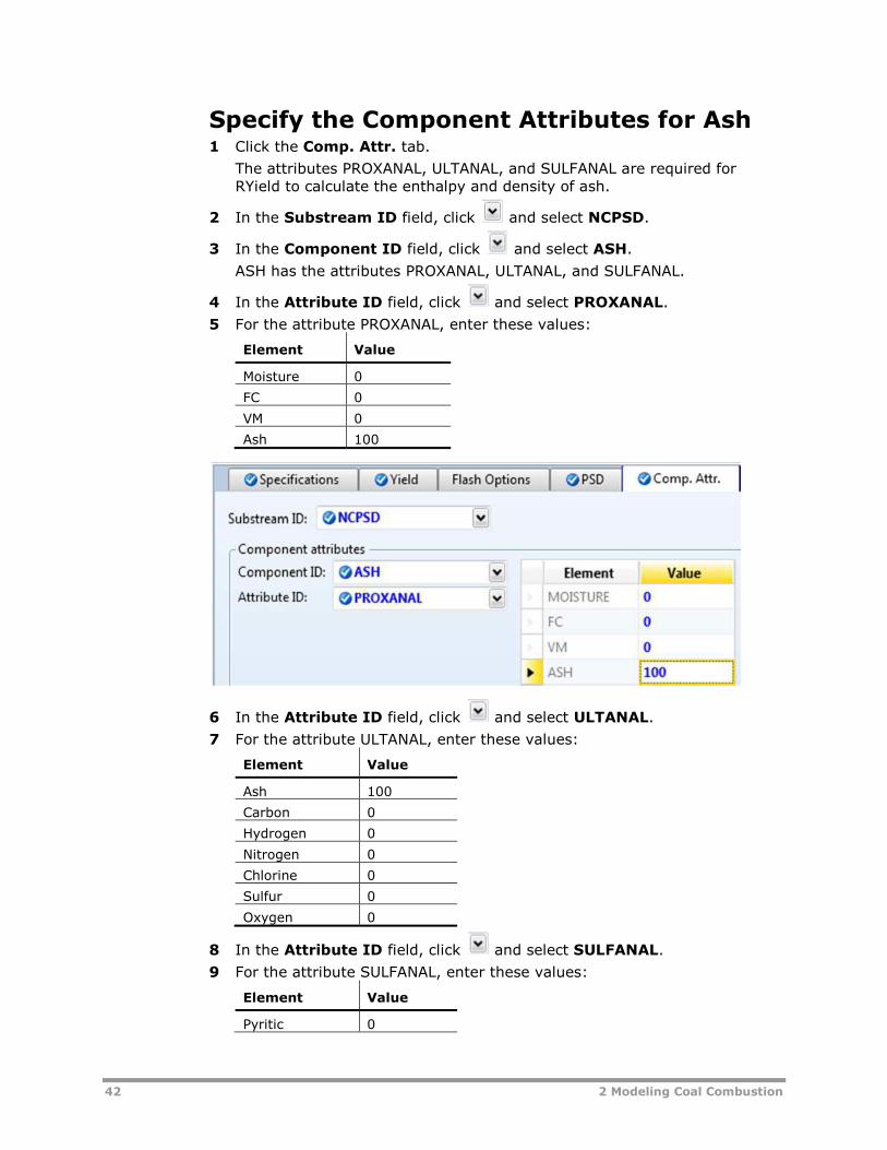
Specify the Component Attributes for Ash1 Click the Comp. Attr. tab.
The attributes PROXANAL, ULTANAL, and SULFANAL are required for
RYield to calculate the enthalpy and density of ash.
2 In the Substream ID field, click and select NCPSD.
3 In the Component ID field, click and select ASH.
ASH has the attributes PROXANAL, ULTANAL, and SULFANAL.
4 In the Attribute ID field, click and select PROXANAL.
5 For the attribute PROXANAL, enter these values:
Element Value
Moisture 0
FC 0
VM 0
Ash 100
6 In the Attribute ID field, click and select ULTANAL.
7 For the attribute ULTANAL, enter these values:
Element Value
Ash 100
Carbon 0
Hydrogen 0
Nitrogen 0
Chlorine 0
Sulfur 0
Oxygen 0
8 In the Attribute ID field, click and select SULFANAL.
9 For the attribute SULFANAL, enter these values:
Element Value
Pyritic 0

2 Modeling Coal Combustion 43
Element Value
Sulfate 0
Organic 0
10 Click to continue.
Specify the Splits for the SSplit Block
The SEPARATE (SSplit) - Input | Specifications sheet appears. SSplit
mixes all of its feed streams, then splits the resulting mixture into two or
more streams according to substream specifications. SSplit operates on
substreams the same way a Sep block operates on components.
In this simulation, the SSplit block provides perfect separation between the
gaseous products of combustion (MIXED substream) and the solid products of
combustion (CIPSD and NCPSD substreams).
1 Enter the following split fraction values for the GASES outlet stream:
Substream Name Value
MIXED 1
CIPSD 0
NCPSD 0
Defining a Calculator BlockYou have completed enough specifications to run the simulation. However,
the yields you specified in the RYield block were only temporary placeholders.
You could directly enter the correct yields on the DECOMP (RYield) - Setup
| Yield sheet. However, by defining a Calculator block to calculate the yields
based on the component attributes of the feed coal, you will be easily able to
run different cases (such as different feed coals).
Create the Calculator Block1 From the Navigation Pane, select Flowsheeting Options | Calculator.
The Calculator object manager appears.
2 Click New to create a new Calculator block.

44 2 Modeling Coal Combustion
The Create New ID dialog box appears with an automatically generated
ID, C-1.
3 In the Create New ID dialog box, enter COMBUST as the ID and click
OK.
Define the Calculator Variables
The COMBUST | Define sheet appears. Use this sheet to access the
flowsheet variables you want to use in the Fortran block. In the simulation in
chapter 1, you accessed individual elements of component attributes. You can
also access component attributes as a vector. In this simulation, access the
ultimate analysis of coal in stream DRY-COAL as a component attribute
vector; also, define variables to access the moisture content of coal and the
yield of each component in the DECOMP block.
4 Create and define the following two variables using category Streams:
Variable
Name
Type Stream Substream Component Attribute Element
ULT Compattr-Vec DRY-COAL NCPSD COAL ULTANAL
WATER Compattr-Var DRY-COAL NCPSD COAL PROXANAL 1
5 Also define the following eight mass yield variables using category
Blocks.
Variable Name ID1 ID2
H2O Type Block-Var
Block DECOMP
Variable MASS-YIELD
for all eight variables.
H2O MIXED
ASH ASH NCPSD
CARB C CIPSD
H2 H2 MIXED
N2 N2 MIXED
CL2 CL2 MIXED
SULF S MIXED
O2 O2 MIXED
6 Click the Calculate tab.

2 Modeling Coal Combustion 45
Specify the Calculations to be Performed
The COMBUST | Calculate sheet appears. ULTANAL is defined as the
ultimate analysis on a dry basis. The variable WATER, defined as the percent
H2O in the PROXANAL for coal, is used to convert the ultimate analysis to a
wet basis. The remaining eight variables (H2O through O2) are defined as the
individual component yields of various species in the RYield block. ULT and
WATER can then be used to calculate the yield of the individual species in the
RYield block.
7 Enter the following Fortran statements:
C FACT IS THE FACTOR TO CONVERT THE ULTIMATE ANALYSIS TO
C A WET BASIS.
FACT = (100 - WATER) / 100
H2O = WATER / 100
ASH = ULT(1) / 100 * FACT
CARB = ULT(2) / 100 * FACT
H2 = ULT(3) / 100 * FACT
N2 = ULT(4) / 100 * FACT
CL2 = ULT(5) / 100 * FACT
SULF = ULT(6) / 100 * FACT
O2 = ULT(7) / 100 * FACT
Note: These calculations assume that the inlet stream consists entirely of
coal. That is true for this problem, but may not be true in other problems
you work with. A good way of handling the multi-component case is to
insert a Sep before the RYield and a Mixer after it, allowing all non-coal
components to bypass the RYield block.
8 Click the Sequence tab.
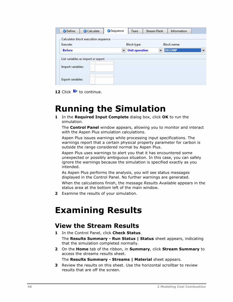
Specify When the Calculator Block Should
be Run
The COMBUST | Sequence sheet appears. Since this Calculator block sets
values in block DECOMP, the Calculator block must execute before DECOMP.
9 In the Execute field, click and select Before.
10 In the Block type field, click and select Unit operation.
11 In the Block name field, click and select DECOMP.
46 2 Modeling Coal Combustion
12 Click to continue.
Running the Simulation1 In the Required Input Complete dialog box, click OK to run the
simulation.
The Control Panel window appears, allowing you to monitor and interact
with the Aspen Plus simulation calculations.
Aspen Plus issues warnings while processing input specifications. The
warnings report that a certain physical property parameter for carbon is
outside the range considered normal by Aspen Plus.
Aspen Plus uses warnings to alert you that it has encountered some
unexpected or possibly ambiguous situation. In this case, you can safely
ignore the warnings because the simulation is specified exactly as you
intended.
As Aspen Plus performs the analysis, you will see status messages
displayed in the Control Panel. No further warnings are generated.
When the calculations finish, the message Results Available appears in the
status area at the bottom left of the main window.
2 Examine the results of your simulation.
Examining Results
View the Stream Results1 In the Control Panel, click Check Status.
The Results Summary - Run Status | Status sheet appears, indicating
that the simulation completed normally.
2 On the Home tab of the ribbon, in Summary, click Stream Summary to
access the streams results sheet.
The Results Summary - Streams | Material sheet appears.
3 Review the results on this sheet. Use the horizontal scrollbar to review
results that are off the screen.

2 Modeling Coal Combustion 47
4 In the Display field, click and select Streams.
5 At the top of each column, click and select INBURNER, AIR,
PRODUCTS, GASES, and SOLIDS.
Results are filled in for each stream as it is specified.
6 Review the results on this sheet. Use the scrollbars to review results that
are off the screen.
Stream PRODUCTS is the outlet of the RGibbs equilibrium reactor that
models the combustion process. Since oxygen appears in stream
PRODUCTS, the combustion process has excess air. An examination of
stream PRODUCTS enables you to determine the most stable products for
each atom in the combustion process:
o SO2 is favored over SO3 and S.
o N2 is favored over NO and NO2.
o CO2 is favored over CO and C (solid).
o HCL is favored over CL2.
7 Click the Heat tab to access the next results sheet.
The Results Summary - Streams | Heat sheet appears. This sheet is
displays the results for heat streams. Examine the results for Q-DECOMP.
The heating value of Q-DECOMP represents the enthalpy change in
breaking down the coal in stream DRY-COAL into its constituent elements.

48 2 Modeling Coal Combustion
View the Block Results
You do not need to view the results for Blocks DRY-REAC and DRY-FLSH,
since they are unchanged from Simulation 1. View the results for blocks
DECOMP, BURN, and SEPARATE.
1 In the Flowsheet, select the DECOMP block.
2 Right-click DECOMP and select Results from the menu.
The DECOMP (RYield) - Results | Summary sheet appears. This sheet
reports the outlet thermodynamic conditions for the block.
3 Click the Balance tab to access the next results sheet.
The DECOMP (RYield) - Results | Balance sheet appears. Use this
sheet to report the mass and energy balance for the block. Because RYield
has a net reaction from nonconventional components to conventional
components, the mass balance for both conventional components and
nonconventional components is out of balance. However, the total mass
balance is in balance.
4 Click the Phase Equilibrium tab to access the next results sheet.
The DECOMP (RYield) - Results | Phase Equilibrium sheet appears.
This sheet indicates that the liquid from the RYield block is a solution of
water and sulfur. In actuality, the sulfur would form a solid at this
temperature. However, this fact does not matter for this simulation,
because the stream (coal broken down into its constituents) does not exist
in a real combustion process. This stream exists only as a mathematical
construct to simplify the specification of the combustion process.

2 Modeling Coal Combustion 49
5 In the Navigation Pane, expand the list of forms for the BURN block and
select Results.
The BURN (RGibbs) - Results | Summary sheet appears. This sheet
reports the outlet thermodynamic conditions of the RGibbs block. The
outlet temperature is the adiabatic flame temperature of the coal with a
fixed amount of excess air.
6 Click the Balance tab to access the next results sheet.
The BURN (RGibbs) - Results | Balance sheet appears.
7 Click the Phase Equilibrium tab to access the next results sheet.
The BURN (RGibbs) - Results | Phase Composition sheet appears.
This sheet displays the mole fraction of components in all phases. In this
case, there is only a vapor phase.
8 Click the Atom Matrix tab to access the next results sheet.
The BURN (RGibbs) - Results | Atom Matrix sheet appears. This sheet
reports the atomic composition for each component.
9 In the Navigation Pane, expand the list of forms for the SEPARATE block
and select Results.
The SEPARATE (SSplit) - Results | Summary sheet appears. This
sheet reports the split fraction for each substream.
Exiting Aspen PlusWhen finished working with this model, exit Aspen Plus as follows:
1 From the ribbon, select File | Exit.
The Aspen Plus dialog box appears.
2 Click Yes to save the simulation.
Aspen Plus saves the simulation as the Aspen Plus Document file,
Solid2.apw, in your default working directory (displayed in the Save in
field).
Note: The chapter 3 simulation uses this run as the starting point.

50 2 Modeling Coal Combustion
3 Modeling Gas-Solid Separators 51
3 Modeling Gas-Solid
Separators
In this simulation, start with the simulation developed in chapter 2, and add a
rigorous gas-solid separation train to separate the ash from the combustion
gases.
You will:
Modify the flowsheet.
Modify the default particle size intervals.
Use solids-handling unit operation models.
Allow about 20 minutes to do this simulation.
Gas-Solid Separation FlowsheetThe process flow diagram and operating conditions for this simulation are
shown in the following figure.
The combustion products from Simulation 2 are fed to a rigorous gas-solid
separation train. Once the products are cooled, solids are removed from the
gases by a cyclone, a fabric filter, and an electrostatic precipitator in series.

52 3 Modeling Gas-Solid Separators
Starting Aspen Plus1 From your desktop, select Start and then select Programs.
2 Select AspenTech | Process Modeling <version> | Aspen Plus |
Aspen Plus <version>.
Opening an Existing Run
If You Completed the Simulation in Chapter
2 and Saved the Simulation
In the Start Using Aspen Plus window, click the link to Solid2.apw under
Recent Models.
If Your Saved File Solid2.apw is Not
Displayed1 Click Open.
The Open dialog box appears.
2 Navigate to the directory that contains your saved file Solid2.apw.
3 Select Solid2.apw in the list of files and click Open.
Note: If you did not create the simulation in Chapter 2, open the backup file
Solid2.bkp in the Examples folder.
To Access the Examples Folder1 Click Open File.
DRIER
Temp = 77 FPres = 14.7 PSICoal Flow = 10000 lb/hrWater Content = 25 wt%
IsobaricAdiabatic
Temp = 270 FPres = 14.7 PSIMass Flow = 50000 lb/hrMole Fraction N2 = 0.999Mole Fraction O2 = 0.001
WET COAL
NITROGEN
EXHAUST
DRY COAL
Water Content = 10 wt%
BURN
RGIBBS
COOLPROD
AIR
CYCLONE
CYCLONE
CYC-GAS
CYC-SOL
Temp = 77 FPres = 14.7 PSIMass Flow = 90000 lb/hrMole Fraction N2 = 0.79Mole Fraction O2 = 0.21
IsobaricAdiabatic
HOTPRODCOOLER
HEATER
Pres = 14.7 psiTemp = 400 F
BAG-FILT
FABFL
FILT-SOL
DP-MAX = 0.5 psi
ESP
ESP
ESP-GAS
ESP-SOL

3 Modeling Gas-Solid Separators 53
The Open dialog box appears.
2 At the left, under Favorites, click Aspen Plus <version> Examples.
By default, this folder contains folders that are provided with Aspen Plus.
3 Double-click the Examples folder, then the GSG_Solids folder.
4 Select Solid2.bkp and click OK.
The process flowsheet from chapter 2 appears:
Saving a Run Under a New
NameBefore creating a new run, create and save a copy of Solid2 with a new Run
ID, Solid3. Then you can make modifications under this new Run ID.
1 From the ribbon, select File | Save As | Aspen Plus Document.
2 In the Save As dialog box, choose the directory where you want to save
the simulation.
3 In the File name field, enter Solid3.
4 Click Save to save the simulation and continue.
Aspen Plus creates a new simulation model, Solid3, which is a copy of the
base case simulation, Solid2.
Modifying the FlowsheetIn the previous simulation, the SSplit block after combustion assumed perfect
separation of the ash from the combustion gases. In the simulation in this
chapter, replace the SSplit block with the following blocks in series: Heater,
Cyclone, FabFl, and ESP.
1 Click and drag a region around the SSplit block and its product streams.
2 Press Delete on the keyboard.
3 In the Confirm Delete dialog box, click OK to delete the group.
4 Draw the flowsheet shown below. (See Getting Started Building and
Running a Process Model, chapter 2, if you need to review how to create a
graphical simulation flowsheet.) Change the name of the product stream
of the RGibbs block and connect it to the new Heater block.

54 3 Modeling Gas-Solid Separators
Changing the Default Particle
Size Distribution
To Update the Title for This Simulation1 From the Navigation Pane, select Setup | Specifications.
The Setup - Specifications | Global sheet appears.
2 Enter the new title Getting Started with Solids - Simulation 3.
Next, modify the system defaults for the size intervals in a particle size
distribution.
To Modify the Particle Size Distribution
Intervals1 From the Navigation Pane, expand the Setup | Solids folder.
2 From the Solids folder, select PSD.

3 Modeling Gas-Solid Separators 55
The Solids - PSD | Mesh sheet appears. Use this sheet to modify the
default particle size distribution.
3 In the No. of intervals field, enter 6.
4 Enter the following six intervals to describe the particle size distribution.
Each Upper value is automatically copied to the next Lower value.
Interval Lower [mu] Upper [mu]
1 0 1
2 1 2
3 2 4
4 4 8
5 8 16
6 16 32
Updating Particle Size Distributions
Previously Entered
Changing the intervals of the particle size distribution (PSD) modifies the
particle size distributions you entered in the previous simulations.
1 In the Navigation Pane, select the Streams | WET-COAL | Input form.
2 Click the NC Solid tab.
The WET-COAL (MATERIAL) - Input | NC Solid sheet appears.
3 Click the arrow in front of Particle Size Distribution to display the data
sheet for PSD.
The original PSD for this stream used size intervals 7 through 10. Since
you just deleted intervals 7 through 10, the PSD is now empty and you
must provide a new PSD. Because the coal is combusted before it reaches
any of the solids-handling unit operation models, an accurate PSD for coal
is not necessary.
4 Enter a value of 1 for the Weight Fraction between 16 and 32 microns.
You must also modify the particle size distribution you specified in the
RYield block DECOMP.
5 In the Navigation Pane, select the Blocks | DECOMP | Setup form.
6 Click the PSD tab.
The DECOMP (RYield) - Setup | PSD sheet appears.
7 In the Substream field, click and select CIPSD.

56 3 Modeling Gas-Solid Separators
8 Enter the following values of Weight fraction for the CIPSD substream.
These particle size distributions are chosen for illustrative purposes only
and are not meant to be typical of an industrial application.
Interval Weight Fraction
1 0.1
2 0.1
3 0.2
4 0.2
5 0.2
6 0.2
9 In the Substream field, click and select NCPSD.
10 Enter the same weight fractions for the particle size distribution for the
NCPSD substream that you entered for the CIPSD substream above.
11 Click to continue.
Specifying the Solids-Handling
BlocksThe BAG-FILT (FabFl) - Input | Specifications sheet appears.
1 Click to find out what must be specified on this sheet.

3 Modeling Gas-Solid Separators 57
2 Close the Completion Status window.
Use the design mode of the fabric filter model (FabFl), not the simulation
mode. Simulation mode determines the capacity of an existing piece of
equipment. Design mode determines the size of a new piece of equipment
with a given capacity.
3 In the Model field, click and select Fabric Filter.
4 In the Mode field, click and select Design.
5 Click to determine what input is required for the FabFl model in design
mode.
In Design mode, FabFl requires a specification for the maximum pressure
drop and Filtration Velocity (the latter of which is an estimate in this
case).
6 Close the Completion Status window.
7 In the Maximum pressure drop field, enter a value of 0.5 psi.
8 Scroll down to the Filtration Velocity field and enter a value of 0.015
m/sec. Be sure to set the units.
9 Click to continue.
The Efficiency sheet appears.
10 In the Separation Efficiency field, click and select Piecewise.
11 Click to continue.

58 3 Modeling Gas-Solid Separators
The COOLER (Heater) - Input | Specifications sheet appears. This
block cools the gas after combustion, allowing the solid ash to be
removed. The Heater block requires two thermodynamic specifications.
12 In the Temperature field, enter 400 F.
13 In the Pressure field, enter 14.7 psia.
14 Click to continue.
The CYCLONE (Cyclone) - Input | Specifications sheet appears.
To Learn About the Cyclone Model Using
Help1 Click anywhere in the CYCLONE (Cyclone) - Input | Specifications
sheet.
2 Press F1 on the keyboard. If a help topic without a blue heading bar
appears, click the link for Sheet Help.
The help for the Cyclone Input Specifications Sheet appears.
3 In the See Also list at the end of the topic, click the Specifying Cyclone
hypertext link.
4 Use the links, scrollbars, and arrow keys to move through the topics.
5 After reviewing the help, close the help window.
6 In the Model field, click and select Cyclone.
7 In the Mode field, click and select Design.
8 In the Calculation method field, click and select Leith-Licht.
9 In the Type field, click and select Stairmand-HE.
10 In the Separation efficiency field, enter a separation efficiency of 0.8.
No further specifications are required for CYCLONE.

3 Modeling Gas-Solid Separators 59
11 Click to continue.
The ESP (ESP) - Input | Specifications sheet appears.
12 In the Model field, click and select Plate.
13 In the Mode field, click and select Design.
14 In the Calculation Method field, click and select Crawford.
15 In the Separation efficiency field, enter 0.995.
16 Click the Dielectric Constant tab.
17 Specify a dielectric constant of 5 for both CIPSD and NCPSD substreams.
Dielectric constant is not needed for the MIXED substream, as it does not
contain solids. The value of the dielectric constant is for illustrative
purposes only.
18 Click to continue.
Running the SimulationThe Required Input Complete dialog box appears.
1 Click OK to run the simulation.
The Control Panel allows you to monitor and interact with the Aspen Plus
simulations calculations. As Aspen Plus performs the simulation, status
messages display in the Control Panel.
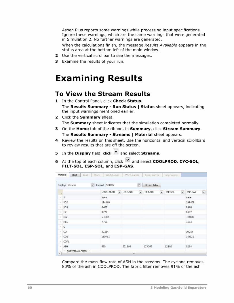
60 3 Modeling Gas-Solid Separators
Aspen Plus reports some warnings while processing input specifications.
Ignore these warnings, which are the same warnings that were generated
in Simulation 2. No further warnings are generated.
When the calculations finish, the message Results Available appears in the
status area at the bottom left of the main window.
2 Use the vertical scrollbar to see the messages.
3 Examine the results of your run.
Examining Results
To View the Stream Results1 In the Control Panel, click Check Status.
The Results Summary - Run Status | Status sheet appears, indicating
the input warnings mentioned earlier.
2 Click the Summary sheet.
The Summary sheet indicates that the simulation completed normally.
3 On the Home tab of the ribbon, in Summary, click Stream Summary.
The Results Summary - Streams | Material sheet appears.
4 Review the results on this sheet. Use the horizontal and vertical scrollbars
to review results that are off the screen.
5 In the Display field, click and select Streams.
6 At the top of each column, click and select COOLPROD, CYC-SOL,
FILT-SOL, ESP-SOL, and ESP-GAS.
Compare the mass flow rate of ASH in the streams. The cyclone removes
80% of the ash in COOLPROD. The fabric filter removes 91% of the ash
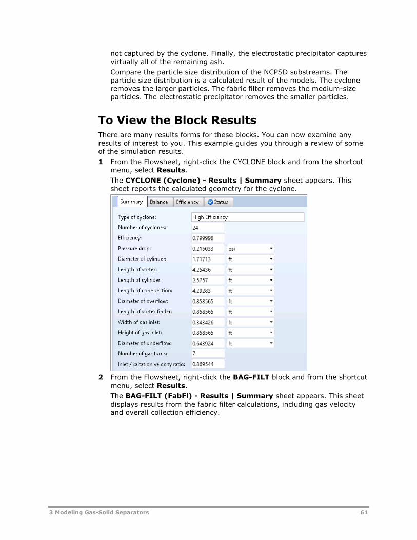
3 Modeling Gas-Solid Separators 61
not captured by the cyclone. Finally, the electrostatic precipitator captures
virtually all of the remaining ash.
Compare the particle size distribution of the NCPSD substreams. The
particle size distribution is a calculated result of the models. The cyclone
removes the larger particles. The fabric filter removes the medium-size
particles. The electrostatic precipitator removes the smaller particles.
To View the Block Results
There are many results forms for these blocks. You can now examine any
results of interest to you. This example guides you through a review of some
of the simulation results.
1 From the Flowsheet, right-click the CYCLONE block and from the shortcut
menu, select Results.
The CYCLONE (Cyclone) - Results | Summary sheet appears. This
sheet reports the calculated geometry for the cyclone.
2 From the Flowsheet, right-click the BAG-FILT block and from the shortcut
menu, select Results.
The BAG-FILT (FabFl) - Results | Summary sheet appears. This sheet
displays results from the fabric filter calculations, including gas velocity
and overall collection efficiency.

62 3 Modeling Gas-Solid Separators
3 From the Flowsheet, right-click the ESP block and from the shortcut
menu, select Results.
The ESP (ESP) - Results | Summary sheet appears. This sheet reports
the geometry, the collection efficiency, and the power requirements of the
electrostatic precipitator.
Exiting Aspen PlusWhen finished working with this model, exit Aspen Plus as follows:
1 From the Navigation Pane, select File | Exit.
The Aspen Plus dialog box appears.
2 Click Yes to save the simulation.
Aspen Plus saves the simulation as the Aspen Plus Document file,
Solid3.apw, in your default working directory (displayed in the Save in
field).
4 Modeling Polymer Recovery 63
4 Modeling Polymer Recovery
In this simulation you will model a simplified polymer washing and drying
process.
You will use:
Component attribute GENANAL to characterize a nonconventional (NC)
component.
The hydrocyclone model (HyCyc).
The counter-current decanter model (CCD).
The cyclone model (Cyclone).
Allow about 30 minutes to do this simulation.
Polymer Recovery FlowsheetThe process flow diagram and operating conditions for this simulation are
shown in the following figure.
The feed stream FEED, a dilute slurry of polymer in acetone, is concentrated
in a hydrocyclone. The concentrated slurry of polymer in acetone is then
washed with water in a countercurrent decanter. The resulting slurry of
polymer in water is dried with nitrogen. The gases from drying are separated
from the solid polymer in a cyclone.

64 4 Modeling Polymer Recovery
Starting Aspen Plus1 From your desktop, select Start and then select Programs.
2 Select AspenTech | Process Modeling <version> | Aspen Plus |
Aspen Plus <version>.
The Start Using Aspen Plus window appears in the main window. In this
simulation, use an Aspen Plus template.
3 Click New.
The New dialog box appears.
Use the New dialog box to specify the template for the new run. Aspen
Plus uses the template you choose to automatically set various defaults
appropriate to your application.
To Specify the Template for the New Run4 Select the Solids with English Units template in the Recently Selected
Templates field.
5 Click Create to apply these options.
It takes a few seconds for Aspen Plus to apply these options.
FEEDHCLONE
HYCYC
ACETONE
Pres = 16 psiTemp = 90 FAcetone Flow = 1000 lb/hrPolymer Flow = 100 lb/hr
Eff = 0.95for 100 microns
CCD
CCD
TO-CCD
WASH-OUT
WASH-H2O
Pres = 16 psiTemp = 200 FH2O Flow = 400 lb/hr
Pres = 15 psi3 stagesMixing eff = 0.9L/S ratio = 2.0
DRIER
MIXER
SLURRY
TO-CYCLHOT-N2
Pres = 16 psiTemp = 350 FN2 Flow = 3000 lb/hr
Pres = 15 psi
CYCLONE
CYCLONE
VENT
Eff = 0.999

4 Modeling Polymer Recovery 65
Specifying ComponentsUse the Components - Specifications | Selection sheet to enter the
components present in the simulation.
The components for this simulation are water, acetone, nitrogen, and
polymer.
1 On the first four Component ID fields, enter H2O, ACETONE, N2, and
POLYMER.
Aspen Plus is able to find WATER, ACETONE and NITROGEN in the
databanks. POLYMER is not found, so the Component name field for
polymer is empty.
By default, Aspen Plus assumes all components have a Type of
Conventional, indicating that they participate in phase equilibrium
calculations. Change the Type for POLYMER to indicate that it is a solid.
Because POLYMER does not have a precise molecular weight, assign
POLYMER the Type Nonconventional.
2 In the Type field for POLYMER, click and select Nonconventional.
3 Click to continue.
The Methods - Specifications | Global sheet appears.
Defining PropertiesUse the Methods - Specifications | Global sheet to select the
thermodynamic methods used to calculate properties such as K-values,
enthalpy, and density. Property methods in Aspen Plus are arranged
according to process types.
Select a Property Method
All property methods use the same physical property models for solid
components. Therefore, the selection of the appropriate property method

66 4 Modeling Polymer Recovery
depends on the components that participate in phase equilibrium. Since
acetone and water form a non-ideal solution, use an activity-coefficient-based
option set. For this simulation, use the NRTL property method.
1 In the Base method field, click and select NRTL.
2 Click to continue.
The Binary Interaction - NRTL-1 (T-DEPENDENT) | Input sheet
appears.
On this sheet, Aspen Plus displays binary interaction parameters for the
NRTL activity coefficient model. Binary parameters are retrieved for all
binary combinations present in the database. If you had data for binary
pairs that are not present in the database, or you wanted to override the
parameters in the database, you could enter your parameters on this
sheet.
Aspen Plus requires you to use this sheet to see what parameters are
available. No further action is required to accept the database values for
the binary interaction parameters. Aspen Plus marks this sheet as
complete as soon as it is displayed.
In this example, parameters are retrieved for the acetone-water pair from
the Aspen Plus VLE-IG databank. Aspen Plus displays the value of the
parameters, and temperature range in which they were regressed. Use
the vertical scrollbar at the bottom right to see all the parameter values.
3 Click to continue.
Specify Nonconventional Component
Property Methods
The Methods - NC Props | Property Methods sheet appears.

4 Modeling Polymer Recovery 67
Specify the methods for Aspen Plus to calculate the enthalpy and density of
the nonconventional component POLYMER. Use the general enthalpy model
(ENTHGEN) and the general density model (DNSTYGEN) in this simulation.
1 In the Model name field for Enthalpy, click and select ENTHGEN.
As soon as you select ENTHGEN, Aspen Plus assigns the attribute
GENANAL to the component POLYMER.
2 In the Model name field for Density, click and select DNSTYGEN.
You use GENANAL to characterize a nonconventional solid in terms of the
weight percent of its constituents. Each nonconventional component may
be characterized by up to 20 constituents.
For example, if you were to characterize paper as a nonconventional
component, you might use the first seven constituents of GENANAL to
represent: cellulose, hemicellulose, lignin, extractives, moisture, and
inerts. Note that there is no way to tell Aspen Plus that the third
constituent of paper represents lignin. You must develop and maintain a
consistent nomenclature outside of Aspen Plus.
In this simulation, use only the first constituent to characterize the
component POLYMER. Thus, POLYMER will be composed of 100%
constituent 1.
Specify Parameters Used to Calculate
POLYMER Properties
Now provide Aspen Plus with the required parameters to calculate enthalpy
and density for the nonconventional component POLYMER.
1 In the Navigation Pane, select Methods | Parameters | Pure
Components.
The Pure Components object manager appears.
2 Click New.

68 4 Modeling Polymer Recovery
The New Pure Component Parameters dialog box appears. The
enthalpy and density parameters for the POLYMER are of a
Nonconventional type.
3 Select the Nonconventional option.
4 Click OK to accept the default ID, NC-1.
The Pure Components - NC-1 | Input sheet appears.
The ENTHGEN model calculates enthalpy from the parameters DHFGEN
and HCGEN. In this simulation DHFGEN (heat of formation) is not required
since POLYMER does not participate in any chemical reactions. You must
provide HCGEN (heat capacity). For this simulation, POLYMER is assumed
to have a constant heat capacity of 0.45 Btu/lb-R.
5 In the Parameter field, click and select HCGEN.
6 In the first field in the Nonconventional component parameter frame,
click and select POLYMER.
7 In the first parameter value field directly below, enter 0.45.
The first four elements of HCGEN are used to calculate the heat capacity
of the first constituent of GENANAL, using the following equation:
32p THCGEN(4)THCGEN(3)THCGEN(2)HCGEN(1)C
HCGEN(2), HCGEN(3) and HCGEN(4) default to zero. Since only the first
constituent of GENANAL will be used to characterize POLYMER, POLYMER
will have a constant heat capacity of 0.45 Btu/lb-R.
If POLYMER were characterized with other constituents, use elements 5
through 8 of HCGEN to calculate the heat capacity of the second
constituent, and so on.
Enter the parameters required for the DNSTYGEN model on this sheet.
DNSTYGEN calculates density for a nonconventional solid from the
DENGEN parameter. For this simulation, POLYMER is assumed to have a
constant density of 80 lb/cuft.
8 In the Parameter field, click and select DENGEN.
9 In the first field in the Nonconventional component parameter frame,
click and select POLYMER.
10 In the first parameter value field, enter 80.

4 Modeling Polymer Recovery 69
11 Click to continue.
The Properties Input Complete dialog box appears.
Correct representation of physical properties is an essential component of
process modeling. For many simulations, the only physical property
specification that you must provide is the selection of an option set. The
Properties Input Complete dialog box shows that the Aspen Plus
physical property system has many optional capabilities that you can use
to increase the accuracy of physical property calculations.
12 Select Go to Simulation environment and click OK to move to the next
required input in the Simulation environment.
Drawing the FlowsheetIn this simulation, begin building the process flowsheet. Since you will enter
your own block and stream IDs, turn off the automatic naming of blocks and
streams, which provide these IDs automatically.
1 From the ribbon, select File | Options.
The Aspen Plus Options dialog box appears.
2 Click Flowsheet on the panel on the left side of the dialog box.
3 Clear the Automatically Assign Block Name with Prefix and
Automatically Assign Stream Name with Prefix check boxes.
4 Click Apply and then OK to apply the changes and close the dialog box.
To Change the Stream Class for the
Simulation1 From the Navigation Pane, click Flowsheet | Section.
The Section object Manager appears.
2 In the Stream class field, click and select MIXNCPSD.
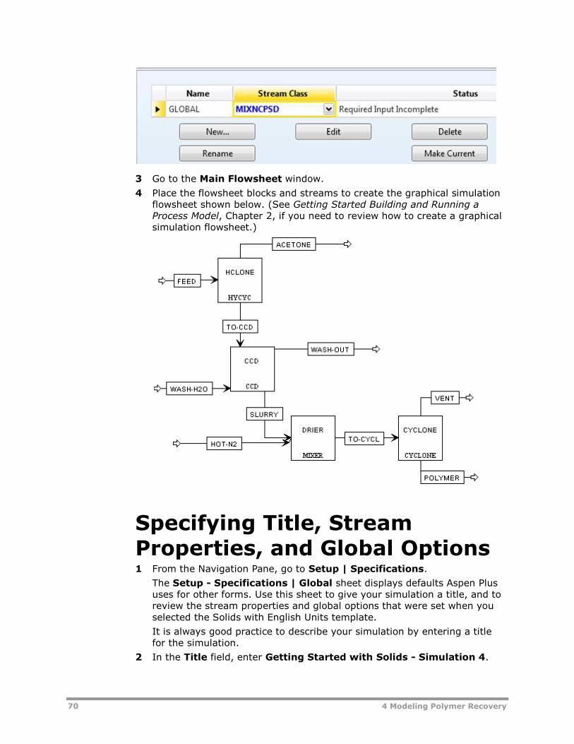
70 4 Modeling Polymer Recovery
3 Go to the Main Flowsheet window.
4 Place the flowsheet blocks and streams to create the graphical simulation
flowsheet shown below. (See Getting Started Building and Running a
Process Model, Chapter 2, if you need to review how to create a graphical
simulation flowsheet.)
Specifying Title, Stream
Properties, and Global Options1 From the Navigation Pane, go to Setup | Specifications.
The Setup - Specifications | Global sheet displays defaults Aspen Plus
uses for other forms. Use this sheet to give your simulation a title, and to
review the stream properties and global options that were set when you
selected the Solids with English Units template.
It is always good practice to describe your simulation by entering a title
for the simulation.
2 In the Title field, enter Getting Started with Solids - Simulation 4.

4 Modeling Polymer Recovery 71
The Solids with English Units template sets the following global defaults
for solids applications:
o ENG units (English Engineering Units).
o Mass Flow basis for all flow inputs.
There are no other changes required on the Setup - Specifications |
Global sheet.
Since you chose the Solids with English Units template when you started
this simulation, Aspen Plus has set the following defaults for calculating
and reporting stream properties:
o The component mass flow rates will be included in the stream report.
o The stream results will be displayed using the SOLIDS Stream Format.
o Property set ALL-SUBS (properties for the entire stream, all
substreams combined) will be reported for each stream.
To Review the Report Options Specified in
the Selected Template1 From the Navigation Pane, select the Setup | Report Options form.
2 Click the Stream tab to view the Setup - Report Options | Stream
sheet.
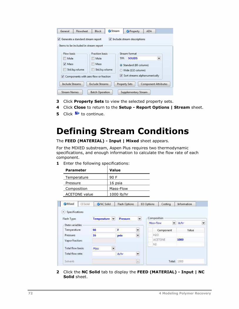
72 4 Modeling Polymer Recovery
3 Click Property Sets to view the selected property sets.
4 Click Close to return to the Setup - Report Options | Stream sheet.
5 Click to continue.
Defining Stream ConditionsThe FEED (MATERIAL) - Input | Mixed sheet appears.
For the MIXED substream, Aspen Plus requires two thermodynamic
specifications, and enough information to calculate the flow rate of each
component.
1 Enter the following specifications:
Parameter Value
Temperature 90 F
Pressure 16 psia
Composition Mass-Flow
ACETONE value 1000 lb/hr
2 Click the NC Solid tab to display the FEED (MATERIAL) - Input | NC
Solid sheet.

4 Modeling Polymer Recovery 73
3 In the Substream name field, click and select NCPSD.
4 Enter the following specifications for the mixed substream:
Parameter Value
Temperature 90 F
Pressure 16 psia
Composition Mass-Flow
POLYMER value 100 lb/hr
5 Click the arrow in front of Particle Size Distribution.
Use this sheet to define the particle size distribution for the POLYMER that
you placed in the NCPSD substream. By default, Aspen Plus uses a particle
size distribution of 10 size ranges covering 20 microns each. The default
size ranges are appropriate for this simulation. On this sheet, enter the
weight fraction of coal in each size range.
6 In the Weight fraction fields, enter the following values:
Interval Weight Fraction
6 0.2
7 0.3
8 0.3
9 0.2
7 Click the arrow in front of Component Attribute.
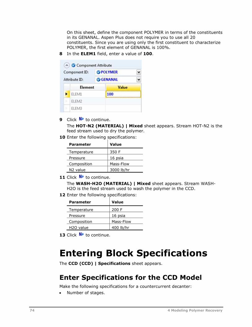
74 4 Modeling Polymer Recovery
On this sheet, define the component POLYMER in terms of the constituents
in its GENANAL. Aspen Plus does not require you to use all 20
constituents. Since you are using only the first constituent to characterize
POLYMER, the first element of GENANAL is 100%.
8 In the ELEM1 field, enter a value of 100.
9 Click to continue.
The HOT-N2 (MATERIAL) | Mixed sheet appears. Stream HOT-N2 is the
feed stream used to dry the polymer.
10 Enter the following specifications:
Parameter Value
Temperature 350 F
Pressure 16 psia
Composition Mass-Flow
N2 value 3000 lb/hr
11 Click to continue.
The WASH-H2O (MATERIAL) | Mixed sheet appears. Stream WASH-
H2O is the feed stream used to wash the polymer in the CCD.
12 Enter the following specifications:
Parameter Value
Temperature 200 F
Pressure 16 psia
Composition Mass-Flow
H2O value 400 lb/hr
13 Click to continue.
Entering Block SpecificationsThe CCD (CCD) | Specifications sheet appears.
Enter Specifications for the CCD Model
Make the following specifications for a countercurrent decanter:
Number of stages.

4 Modeling Polymer Recovery 75
Operating pressure.
Mixing efficiency.
Liquid/solid ratio.
If you do not provide mixing efficiency or liquid/solid ratio for all stages,
Aspen Plus determines the values for missing stages by linear interpolation. If
you provide only a single value for mixing efficiency or liquid/solid ratio,
Aspen Plus uses that value for all stages.
By default, Aspen Plus assumes each stage of a countercurrent decanter to be
adiabatic. Alternatively, you could specify a temperature, a heat duty, or a
heat transfer coefficient for each stage.
1 Enter the following operating conditions:
Field Value
Number of stages 3
Pressure 15 psia
2 For the stage profiles, enter:
Field Value
Stage 1
Mixing efficiency 0.9
Liquid-to-solid mass ratio 2
3 Click the Streams tab.
The CCD (CCD) | Streams sheet describes the connections of the
streams to the stages of the CCD. It is already complete.
4 Click to continue.
The CYCLONE (Cyclone) | Specifications sheet appears.
To Learn More about the Cyclone Model
Using Help1 Click anywhere on the CYCLONE (Cyclone) | Specifications sheet.
2 Press F1. If a help window without a blue heading bar appears, click the
link for Sheet Help.

76 4 Modeling Polymer Recovery
The help for the Cyclone Input Specifications Sheet appears.
3 In the list of See Also links, click the Specifying Cyclone hypertext link.
4 Use the links, scrollbars, and arrow keys to move through the topics.
5 After reviewing the help, close the help window.
You can use the Cyclone model in simulation mode or design mode. In this
simulation, use Cyclone in design mode. Aspen Plus will determine the
dimensions and the number of cyclones required to achieve a specified
efficiency for solids removal.
Enter Specifications for the Cyclone Model
1 In the Model field, click and select Cyclone.
2 In the Mode field, click and select Design.
3 In the Calculation method field, click and select Leith-Licht.
4 In the Type field, click and select Stairmand-HE.
5 In the Separation efficiency field, enter a separation efficiency of
0.999.
6 From the Navigation Pane, click Blocks | DRIER.
The DRIER (Mixer) | Flash Options sheet appears. The sheet is marked
complete, since there are no specifications required for a Mixer block.
However, Aspen Plus does allow the pressure of the Mixer as an optional
specification.
To Specify That the Mixer Block DRIER
Operates at 15 psia1 In the Pressure field, enter 15 psia.
2 Click to continue.
The HCLONE (HyCyc) | Specifications sheet appears.

4 Modeling Polymer Recovery 77
Enter Specifications for the HyCyc Model1 Click anywhere on the Specifications sheet.
2 Press F1.
3 Use the links, scrollbars, and arrow keys to move through the topics.
4 After reviewing the help, close the help window.
You can use HyCyc in simulation mode or design mode. In this example, use
HyCyc in design mode. In design mode, make the following specifications:
Particle size for design efficiency.
Design separation efficiency.
Maximum diameter of the hydrocyclone.
Maximum pressure drop.
5 In the Model field, click and select Hydrocyclone.
6 In the Mode field, click and select Design.
7 In the Efficiency Correlation field, click and select Bradley.
8 In the Type field, click and select User-specified ratios.
9 Enter the following specifications:
Field Value
Diameter of solid particles 100 mu (microns)
Separation efficiency 0.95
Maximum diameter 1.5 ft
Maximum pressure drop 5 psi
Be sure to specify the units of measure for the particle diameter.
To help concentrate the solid slurry, change the default geometry of the
hydroclone. Increasing the size of the overflow diameter increases the
amount of liquid product in stream ACETONE. Specify that the ratio of the
overflow diameter to the hydroclone diameter be equal to 0.3.
10 Click the Ratios tab.

78 4 Modeling Polymer Recovery
11 In the Inlet Configuration field, click and select Round.
12 In the Diameter of overflow field, enter 0.3.
13 Click to continue.
The Required Input Complete dialog box appears.
Running the SimulationYou have now entered the data and specifications for this simulation.
1 Click OK to run the simulation.
The Control Panel allows you to monitor and interact with the Aspen Plus
simulations calculations. As Aspen Plus performs the simulation, status
messages display in the Control Panel.
GENANAL is defined as having 20 constituents. If you only use a portion of
the constituents available in GENANAL, Aspen Plus generates a warning.
Since you need only one element in GENANAL for this simulation, ignore
this warning. The remainder of the simulation completes without warnings
or errors.
When the calculations finish, the message Results Available appears in the
status area at the bottom right of the main window.
2 Use the vertical scrollbar to see the messages.
3 Examine the results of your run.
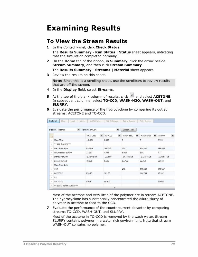
4 Modeling Polymer Recovery 79
Examining Results
To View the Stream Results1 In the Control Panel, click Check Status.
The Results Summary - Run Status | Status sheet appears, indicating
that the simulation completed normally.
2 On the Home tab of the ribbon, in Summary, click the arrow beside
Stream Summary, and then click Stream Summary.
The Results Summary - Streams | Material sheet appears.
3 Review the results on this sheet.
Note: Since this is a scrolling sheet, use the scrollbars to review results
that are off the screen.
4 In the Display field, select Streams.
5 At the top of the blank column of results, click and select ACETONE.
In subsequent columns, select TO-CCD, WASH-H2O, WASH-OUT, and
SLURRY.
6 Evaluate the performance of the hydrocyclone by comparing its outlet
streams: ACETONE and TO-CCD.
Most of the acetone and very little of the polymer are in stream ACETONE.
The hydrocyclone has substantially concentrated the dilute slurry of
polymer in acetone to feed to the CCD.
7 Evaluate the performance of the countercurrent decanter by comparing
streams TO-CCD, WASH-OUT, and SLURRY.
Most of the acetone in TO-CCD is removed by the wash water. Stream
SLURRY contains polymer in a water rich environment. Note that stream
WASH-OUT contains no polymer.

80 4 Modeling Polymer Recovery
8 After the SLURRY column, click and select the following streams HOT-
N2, TO-CYCL, VENT, and POLYMER.
The DRIER block operates by mixing streams SLURRY and HOT-N2. There
is enough hot nitrogen to adiabatically evaporate all of the liquid in stream
SLURRY (VFrac + SFrac =1 in stream TO-CYCL).
The CYCLONE block separates the solid polymer from the gas. Because the
Cyclone model neglects the interstitial flow of gas in the separated solids,
stream POLYMER has no flow of H2O, ACETONE, or N2.
To View the Block Results1 In the Flowsheet, right-click the CCD block. From the shortcut menu,
select Results.
The CCD (CCD) - Results | Summary sheet appears. This sheet displays
summary flow and temperature information for the first and last stages.
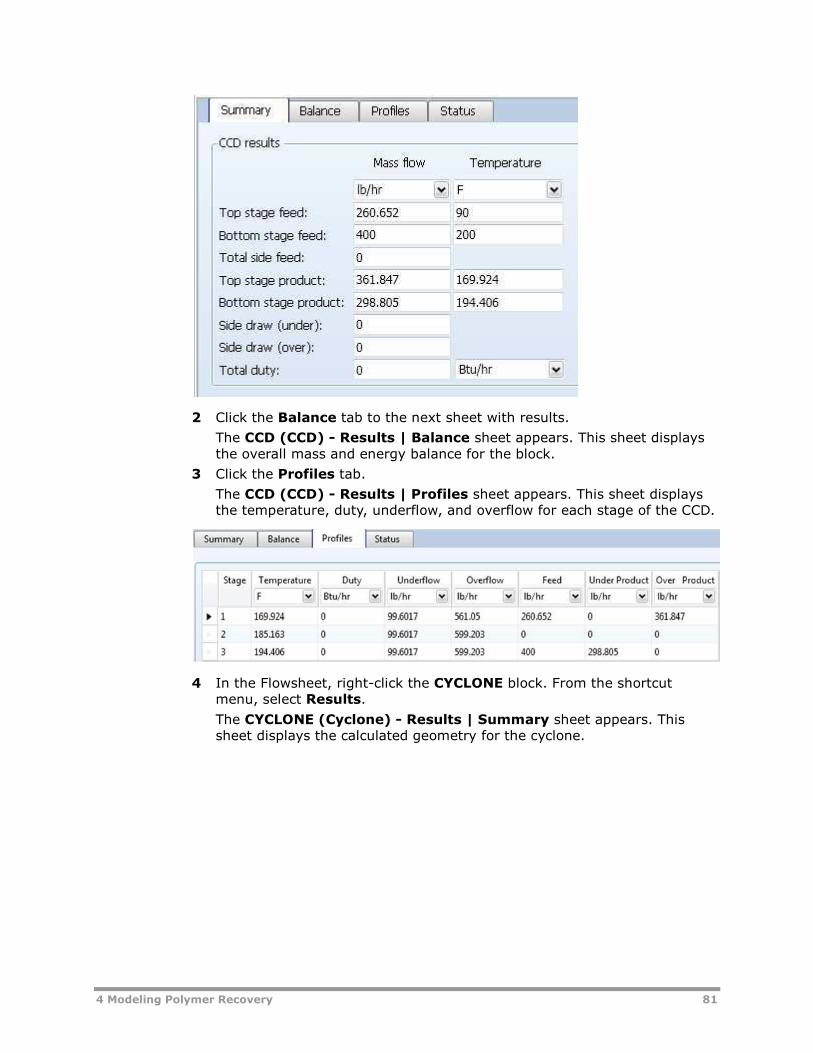
4 Modeling Polymer Recovery 81
2 Click the Balance tab to the next sheet with results.
The CCD (CCD) - Results | Balance sheet appears. This sheet displays
the overall mass and energy balance for the block.
3 Click the Profiles tab.
The CCD (CCD) - Results | Profiles sheet appears. This sheet displays
the temperature, duty, underflow, and overflow for each stage of the CCD.
4 In the Flowsheet, right-click the CYCLONE block. From the shortcut
menu, select Results.
The CYCLONE (Cyclone) - Results | Summary sheet appears. This
sheet displays the calculated geometry for the cyclone.

82 4 Modeling Polymer Recovery
5 Click the Balance tab to move to the next sheet with results.
The CYCLONE (Cyclone) - Results | Balance sheet appears. This sheet
displays the overall mass and energy balance for the block.
6 In the Flowsheet, right-click the DRIER block. From the shortcut menu,
select Results.
The DRIER (Mixer) - Results | Summary sheet appears. This sheet
displays the outlet thermodynamic conditions for the block.
7 Click the Balance tab to move to the next sheet with results.
The DRIER (Mixer) - Results | Balance sheet appears. This sheet
displays the overall mass and energy balance for the block.
8 In the Flowsheet, right-click the HCLONE block. From the shortcut menu,
select Results.
The HCLONE (HyCyc) - Results | Summary sheet appears. This sheet
displays the calculated geometry for the block.

4 Modeling Polymer Recovery 83
Exiting Aspen PlusWhen you are finished working with this model, you can exit Aspen Plus as
follows:
1 From the ribbon, select File | Exit.
The Aspen Plus dialog box appears.
2 Click Yes to save the simulation.
3 In the Save As dialog box, enter Solid4 in the File name box.
Aspen Plus saves the simulation as the Aspen Plus Document file,
Solid4.apw, in your default working directory (displayed in the Save in
box).
This simulation is delivered as backup file solid4 in the online Aspen Plus
Examples Library. You can use this backup file to check your results.