Post-hoc Uncertainty Calibration for Domain Drift Scenarios

Christian Tomani1, Sebastian Gruber3,4,5,*, Muhammed Ebrar Erdem2,Daniel Cremers1, Florian Buettner2,3,4,5,*

1Technical University of Munich2Siemens AG 3 German Cancer Consortium

4 German Cancer Research Center Heidelberg 5 Frankfurt University{christian.tomani, cremers}@tum.de,

{sebastian.gruber, muhammed.erdem, buettner.florian}@siemens.com

Abstract

We address the problem of uncertainty calibration.While standard deep neural networks typically yield uncal-ibrated predictions, calibrated confidence scores that arerepresentative of the true likelihood of a prediction can beachieved using post-hoc calibration methods. However, todate, the focus of these approaches has been on in-domaincalibration. Our contribution is two-fold. First, we showthat existing post-hoc calibration methods yield highly over-confident predictions under domain shift. Second, we intro-duce a simple strategy where perturbations are applied tosamples in the validation set before performing the post-hoccalibration step. In extensive experiments, we demonstratethat this perturbation step results in substantially better cal-ibration under domain shift on a wide range of architecturesand modelling tasks.

1. Introduction

1.1. Towards calibrated classifiers

Due to their high predictive power, deep neural networksare increasingly being used as part of decision making sys-tems in real world applications. However, such systemsrequire not only high accuracy, but also reliable and cali-brated uncertainty estimates. A classifier is calibrated, ifthe confidence of predictions matches the probability of be-ing correct for all confidence levels [4]. Especially in safetycritical applications in medicine where average case perfor-mance is insufficient, but also in dynamically changing en-vironments in industry, practitioners need to have access toreliable predictive uncertainty during the entire life-cycle ofthe model. This means confidence scores (or predictive un-certainty) should be well calibrated not only for in-domain

* Work done for Siemens AG

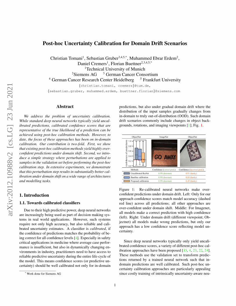
predictions, but also under gradual domain drift where thedistribution of the input samples gradually changes fromin-domain to truly out-of-distribution (OOD). Such domaindrift scenarios commonly include changes in object back-grounds, rotations, and imaging viewpoints [1]; Fig. 1.

Methods Confidence (correct pred.) Confidence (incorrect pred.)

Uncalibrated ResNet 0.99 (doormat) 0.91 (hanky)

Baseline calibration 0.99 (doormat) 0.85 (hanky)

Proposed calibration 0.99 (doormat) 0.45 (hanky)

ObjectNet ImageNet ObjectNet

Figure 1: Re-calibrated neural networks make over-confident predictions under domain drift. Left: Only for ourapproach confidence scores match model accuracy (dashedred line) across all predictions; all other approaches areover-confident under domain shift. Middle: For Imagenet,all models make a correct prediction with high confidence(left). Right: Under domain drift (different viewpoint; Ob-jectnet) all models make wrong predictions, but only ourapproach has a low confidence score reflecting model un-certainty.

Since deep neural networks typically only yield uncali-brated confidence scores, a variety of different post-hoc cal-ibration approaches have been proposed [15, 4, 23, 22, 24].These methods use the validation set to transform predic-tions returned by a trained neural network such that in-domain predictions are well calibrated. Such post-hoc un-certainty calibration approaches are particularly appealingsince costly training of intrinsically uncertainty-aware neu-

1

arX

iv:2

012.

1098

8v2

[cs

.LG

] 2

3 Ju

n 20

21

ral networks can be avoided.Current efforts to systematically quantify the quality of pre-dictive uncertainties have focused on assessing model cali-bration for in-domain predictions. Here, post-processing inform of temperature scaling has shown great promise andGuo et al. [4] illustrated that this approach yields well cal-ibrated predictions for a wide range of model architectures.More recently, more complex combinations of paramet-ric and non-parametric methods have been proposed [24].However, little attention has been paid to uncertainty cal-ibration under domain drift and no comprehensive analy-sis of the performance of post-hoc uncertainty calibrationmethods under domain drift exists.

1.2. Contribution

In this work we focus on the task of post-hoc uncertaintycalibration under domain drift scenarios and make the fol-lowing contributions:

• We first show that neural networks yield overconfidentpredictions under domain shift even after re-calibrationusing existing post-hoc calibrators.

• We generalise existing post-hoc calibration methodsby transforming the validation set before performingthe post-hoc calibration step.

• We demonstrate that our approach results in substan-tially better calibration under domain shift on a widerange of architectures and image data sets.

In addition to the contributions above, our code ismade available at https://github.com/tochris/calibration-domain-drift.

2. Related workIn this section, we review existing approaches towards

neural networks with calibrated predictive uncertainty. Thefocus of this work is on post-hoc calibration methods, whichwe review in detail. These approaches can broadly bedivided into 2 categories: accuracy-preserving methods,where the ranking of confidence scores across classes re-main unchanged and those where the ranking, and thusaccuracy, can change. Other related work includes in-trinsically uncertainty-aware neural networks and out-of-distribution detection methods.

2.1. Post-processing methods

A popular approach towards well-calibrated predictionsare post-hoc calibration methods where a validation set,drawn from the generative distribution of the training dataπ(X,Y ), is used to rescale the outputs returned by a trainedneural network such that in-domain predictions are well cal-ibrated. A variety of parametric, as well as non-parametric

methods exist. We first review non-parametric methodsthat do not preserve accuracy. A simple but popular non-parametric post-processing approach is histogram binning[22]. In brief, all uncalibrated confidence scores Pl are par-titioned into M bins (with borders typically chosen suchthat either all bins are of equal size or contain the samenumber of samples). Next, a calibrated score Qm that isdetermined by optimizing a bin-wise squared loss on thevalidation set, is assigned to each bin. For each new predic-tion, the uncalibrated confidence score Ppr is then replacedby the calibrated score associated with the bin Ppr falls into.Popular extensions to histogram binning are isotonic regres-sion [23] and Bayesian Binning into Quantiles (BBQ) [12].For isotonic regression (IR), uncalibrated confidence scoresare divided into M intervals and a piecewise constant func-tion f is fitted on the validation set to transform uncalibratedoutputs to calibrated scores. BBQ is a Bayesian generalisa-tion of histogram binning based on the concept of Bayesianmodel averaging.In addition to these non-parametric approaches, also para-metric alternatives for post-processing confidence scoresexist. Platt scaling [15] is an approach for transforming thenon-probabilistic outputs (logits) zi ∈ R of a binary classi-fier to calibrated confidence scores. More specifically, thelogits are transformed to calibrated confidence scores Qi

using logistic regression Qi = σ(azi + b), where σ is thesigmoid function and the two parameters a and b are fittedby optimising the negative log-likelihood of the validationset.Guo et al. [4] have proposed Temperature Scaling (TS), asimple generalisation of Platt scaling to the multi-class case,where a single scalar parameter T is used to re-scale the log-its of a trained neural network. In the case of C-class clas-sification, the logits are a C-dimensional vector zi ∈ RC ,which are typically transformed into confidence scores Pi

using the softmax function σSM . For temperature scaling,logits are rescaled with temperature T and transformed intocalibrated confidence scores Qi using the softmax functionas

Qi = maxcσSM (zi/T )(c) (1)

T is learned by minimizing the negative log likelihood ofthe validation set. In contrast to the non-parametric meth-ods introduced above or other multi-class generalisationsof Platt scaling such as vector scaling or matrix scaling,Temperature Scaling has the advantage that it does notchange the accuracy of the trained neural network. Sincere-scaling does not affect the ranking of the logits, also themaximum of the softmax function remains unchanged.More recently, Zhang et al. [24] have proposed to combineto combine parametric methods with non-parametricmethods, in particular they suggest it can be beneficialto perform IR after a TS step (TS-IR). In addition, theyintroduced an accuracy-preserving version of IR, termed

2

IRM and an ensemble version of temperature scaling,called ETS.

2.2. Intrinsically uncertainty-aware neural net-works

A variety of approaches towards intrinsicallyuncertainty-aware neural networks exist, includingprobabilistic and non-probabilistic approaches. In recentyears, a lot of research effort has been put into trainingBayesian neural networks. Since exact inference is un-tractable, a range of approaches for approximate inferencehas been proposed, [3, 21]. A popular non-probabilisticalternative is Deep Ensembles [10], where an ensemble ofnetworks is trained using adversarial examples, yieldingsmooth predictions with meaningful predictive uncertainty.Other non-probabilistic alternatives include, e.g., [17, 20].While a comprehensive analysis of the performance ofpost-hoc calibration methods is missing for domain-driftscenarios, recently Ovadia et al. [13] have presented a firstcomprehensive evaluation of calibration under domain driftfor intrinsically uncertainty-aware neural networks andhave shown that the quality of predictive uncertainties, i.e.model calibration, decreases with increasing dataset shift,regardless of method.

2.3. Other related work

Orthogonal approaches have been proposed where trustscores and other measures for out-of-distribution detectionare derived to detect truly OOD samples, often also basedon trained networks and with access to a known OODset [11, 8, 14]. However, rather than only detecting trulyOOD samples, in this work, we are interested in calibratedconfidence scores matching model accuracy at all stagesof domain drift, from in-domain samples to truly OODsamples.

3. Problem setup and definitionsLet X ∈ RD and Y ∈ {1, . . . , C} be random variables

that denote the D-dimensional input and labels in a classifi-cation task with C classes with a ground truth joint distribu-tion π(X,Y ) = π(Y |X)π(X). The dataset D consists ofN i.i.d.samples D = {(Xn, Yn)}Nn=1 drawn from π(X,Y ).Let h(X) = (Y , P ) be the output of a neural network clas-sifier h predicting a class Y and associated confidence Pbased onX . Here, we are interested in the quality of predic-tive uncertainty (i.e. confidence scores P ) not only on testdata from the generative distribution of the training data D,π(X,Y ), but also under dataset shift, that is test data froma distribution ρ(X,Y ) 6= π(X,Y ). More specifically, weinvestigate domain drift scenarios where the distribution ofsamples seen by a model gradually moves away from the

training distribution π(X,Y ) (in an unknown fashion) untilit reaches truly OOD levels.We assess the quality of the confidence scores using the no-tion of calibration. We define perfect calibration such thataccuracy and confidence match for all confidence levels:

P(Y = Y |P = p) = p, ∀p ∈ [0, 1] (2)

This directly leads to a definition of miss-calibration as thedifference in expectation between confidence and accuracy:Based on equation 3 it is straight-forward to define miss-calibration as the difference in expectation between confi-dence and accuracy:

EP

[∣∣P(Y = Y |P = p)− p∣∣] (3)

The expected calibration error (ECE) [12] is a scalarsummary measure estimating miss-calibration by approxi-mating equation 3 based on predictions, confidence scoresand ground truth labels {(Yl, Yl, Pl)}Ll=1 of a finite num-ber of L samples. ECE is computed by first partition-ing all L confidence scores Pl into M equally sized binsof size 1/M and computing accuracy and average con-fidence of each bin. Let Bm be the set of indices ofsamples whose confidence falls into its associated intervalIm =

(m−1M , m

M

]. conf(Bm) = 1/|Bm|

∑i∈Bm

Pi andacc(Bm) = 1/|Bm|

∑i∈Bm

1(Yi = Yi) are the averageconfidence and accuracy associated with Bm, respectively.The ECE is then computed as

ECE =

M∑m=1

|Bm|n

∣∣acc(Bm)− conf(Bm)∣∣ (4)

It can be shown that ECE is directly connected to miss-calibration, as ECE using M bins converges to the M -termRiemann-Stieltjes sum of eq. 3 [4].

4. Uncertainty calibration under domain drift4.1. Baseline methods and experimental setup

We assess the performance of the following post-hoc un-certainty calibration methods in domain drift scenarios:

• Base: Uncalibrated baseline model

• Temperature scaling (TS) [4] and Ensemble Tempera-ture Scaling (ETS) [24]

• Isotonic Regression (IR) [23]

• Accuracy preserving version of Isotonic Regression(IRM) [24]

• Composite model combining Temperature Scaling andIsotonic Regression (TS-IR) [24]

3

We quantify calibration under domain shift for 28 distinctperturbation types not seen during training, including 9affine transformations, 19 image perturbations introducedby [6] and a dedicated bias-controlled dataset [1]. Eachperturbation strategy mimics a scenario where the data ofa deployed model encounters stems from a distribution thatgradually shifts away from the training distribution in a dif-ferent manner. For each model and each perturbation, wecompute the micro-averaged ECE by first perturbing eachsample in the test set at 10 different levels and then calcu-lating the overall ECE across all samples; we denote rela-tive perturbation strength as epsilon. A common manifesta-tion of dataset shift in real-world applications is a change inobject backgrounds, rotations, and imaging viewpoints. Inorder to quantify the expected calibration error under thosescenarios, we use Objectnet, a recently proposed large-scalebias-controlled dataset [1]. The Objectnet dataset contains50,000 test images with a total of 313 classes, of which113 overlap with Imagenet. Uncertainty calibration underdomain drift was evaluated for CIFAR-10 based on affinetransformations, and for Imagenet based on the perturba-tions introduced by [6] as well as the overlapping classes inObjectnet.In addition, we quantify the quality of predictive uncertaintyfor truly OOD scenarios by computing the predictive en-tropy and distribution of confidence scores. We use com-plete OOD datasets as well as data perturbed at the highestlevel. In these scenarios we expect entropy to reach maxi-mum levels, since the model should transparently commu-nicate it ”does not know” via low and unbiased confidencescores.

4.2. Improving calibration under domain drift

Existing methods for post-hoc uncertainty calibration arebased on a validation set, which is drawn from the samegenerative distribution π(X,Y ) as the training set and thetest set. Using these data to optimize a post-hoc calibra-tion method results in low calibration errors for data drawnfrom π(X,Y ). If we would like to generalise this ap-proach to calibration under domain drift, we need accessto samples from the generative distribution along the axisof domain drift. However, such robustness under domaindrift is a challenging requirement since in practice for a D-dimensional input domain drift can occur in any of the 2D

directions in {−1, 1}D, and to any degree. Manifestationsof such domain shifts include for example changes in view-point (Fig. 1), lighting condition, object rotation or back-ground.To obtain a transformed validation set representing ageneric domain shift, we therefore sample domain drift sce-narios by randomly choosing direction and magnitude ofthe domain drift. We use these scenarios to perturb the val-idation set and, taken together, simulate a generic domain

0 2 4 6 8Epsilon

0.25

0.50

0.75

1.00

1.25

Entropy

0.2

0.4

0.6

0.8

Accuracy

(a) Accuracy and entropy forCIFAR-10 data

0 2 4 6 8Epsilon

0.0

0.2

0.4

0.6

ECE

(b) ECE for CIFAR-10 data

Figure 2: Model performance in terms of accuracy, entropyand expected calibration error for CIFAR-10 data for per-turbation shear. (a) As expected accuracy degrades with in-creasing perturbation to almost random levels for all mod-els. (b) While entropy increases with increasing perturba-tion strength Epsilon for all models, ECE also increases forall models, indicating a mis-match between confidence andaccuracy.

Base TS ETS TS-IR IR IRM0.0

0.1

0.2

0.3

ECE

(a) CIFAR-10

Base TS ETS TS-IR IR IRM0.00

0.05

0.10

0.15

ECE

(b) Imagenet

Figure 3: Mean expected calibration error, averaged overall test scenarios and levels of domain drift. Using our pro-posed calibration approach improves the overall calibrationerror for all post-hoc calibrators.

drift. More specifically, we first choose a random directiondt ∈ {−1, 1}D. Next, we sample from a set of 10 noise lev-els ε covering the entire spectrum from in-domain to trulyout-of domain. Each noise level corresponds to the varianceof a Gaussian which in turn is used to sample the magnitudeof domain drift. Since level and direction of domain shiftare not known a priori, we argue that an image transforma-tion using such Gaussian noise results in a generic valida-tion set in the spirit of the central limit theorem: we emulatecomplex domain shifts in the real world by performing ad-ditive random image transformations, which in turn can beapproximated by a Gaussian distribution.We optimise ε in a dataset-specific manner such that theaccuracy of the pre-trained model decreases linearly in 10steps to random levels (See Appendix for detailed algo-rithm).

In summary, we sample a domain shift scenario usingGaussian noise for each sample in the validation set, therebygenerating a perturbed validation set. We then tune a given

4

Base TS ETS TS-IR IR IRM TS-P ETS-P TS-IR-P IR-P IRM-P

CIFAR VGG19 0.323 0.158 0.152 0.173 0.176 0.167 0.053 0.057 0.051 0.049 0.044CIFAR ResNet50 0.202 0.176 0.171 0.191 0.190 0.179 0.083 0.090 0.092 0.093 0.076CIFAR DenseNet121 0.206 0.151 0.145 0.166 0.168 0.152 0.135 0.122 0.103 0.088 0.120CIFAR MobileNetv2 0.159 0.150 0.141 0.165 0.165 0.147 0.107 0.125 0.094 0.079 0.108

ImgNet ResNet50 0.130 0.049 0.064 0.134 0.142 0.072 0.050 0.041 0.033 0.037 0.041ImgNet ResNet152 0.129 0.043 0.049 0.127 0.135 0.062 0.037 0.034 0.028 0.039 0.045ImgNet VGG19 0.057 0.045 0.047 0.120 0.122 0.051 0.093 0.075 0.064 0.029 0.047ImgNet Den.Net169 0.117 0.044 0.040 0.127 0.133 0.057 0.024 0.023 0.026 0.045 0.050ImgNet Eff.NetB7 0.092 0.135 0.085 0.131 0.132 0.074 0.074 0.047 0.038 0.049 0.058ImgNet Xception 0.205 0.068 0.042 0.109 0.130 0.076 0.060 0.031 0.031 0.101 0.101ImgNet Mob.Netv2 0.063 0.143 0.114 0.186 0.181 0.107 0.099 0.074 0.066 0.046 0.069

Table 1: Mean expected calibration error across all test domain drift scenarios (affine transformations for CIFAR-10 and per-turbations proposed in [6] for Imagenet). For all architectures our approach of using a perturbed validation set outperformedbaseline post-hoc calibrators

post-hoc uncertainty calibration method based on this per-turbed validation set and obtain confidence scores that arecalibrated under domain drift. All in all, we simulate do-main drift scenarios and use the resulting perturbed vali-dation set to tune existing post-hoc uncertainty calibrationmethods. We hypothesize that this facilitates calibrated pre-dictions of neural networks under domain drift.We refer to tuning a post-hoc calibrator using the perturbedvalidation set by a suffix ”-P”, e.g. IR-P stands for IsotonicRegression tuned on the perturbed validation set.

5. Experiments and resultsWe first illustrate limitations of post-hoc uncertainty cal-

ibration methods in domain drift scenarios using CIFAR-10.We show that while excellent in-domain calibration can beachieved using standard baselines, the quality of uncertaintydecreases with increasing domain shift for all methods, re-sulting in highly overconfident predictions for images faraway from the training domain.Next, we show on a variety of architectures and datasets thatreplacing the validation set by a transformed validation setas outlined in section 4.2, substantially improves calibrationunder domain shift. We further assess the effect of our newapproach on in-domain calibration and demonstrate that forselected post-hoc calibration methods, in-domain calibra-tion can be maintained at competitive levels. Finally, weshow that our tuning approach results in better uncertaintyawareness in truly OOD settings.

5.1. Post-hoc calibration results in overconfidentpredictions under domain drift

We tuned all post-hoc calibration baseline methods onthe CIFAR-10 validation set and first assessed in-domaincalibration on the test set. As expected, calibration im-

proves for all baselines over the uncalibrated network pre-dictions in this in-domain setting. Next, we assessed cal-ibration under domain drift by generating a perturbed testwhere we apply different perturbations (e.g. rotation, shear,zoom) to the images. We increased perturbation strength(i.e. shear) in 9 steps until reaching random accuracy. Fig-ure 2 illustrates, that while entropy increases with intensi-fying shear for all models, ECE also increases for the entireset of models. This reveals a mis-match between confidenceand accuracy that increases with increasing domain drift.

5.2. Perturbed validation sets improve calibrationunder domain drift

Next, we systematically assessed whether calibration un-der domain drift can be improved by tuning post-hoc cali-bration methods on a transformed validation set. To thisend, we calibrate various neural network architectures onCIFAR-10 and Imagenet. For CIFAR-10, we first trainVGG19 [18], ResNet50 [5], DenseNet121 [7] and Mo-bileNetv2 [16] models. For Imagenet we used 7 pre-trainedmodels provided as part of tensorflow, namely ResNet50,ResNet152, VGG19, DenseNet169, EfficientNetB7 [19],Xception [2] and MobileNetv2.For all neural networks we then tuned 2 sets of post-hoccalibrators: one set was tuned in a standard manner basedon the validation set, the second set was tuned with the pro-posed method based on the perturbed validation set. Wethen evaluate both sets of calibrators under various domaindrift scenarios that were not seen during training, as well asin terms of in-domain calibration.We observed that for all post-hoc calibrators tuning on aperturbed validation set resulted in an overall lower cali-bration error when testing across all domain drift scenarios,Table 1, Fig. 3). Figure 4 illustrates for VGG19 trained on

5

xyzoom

yshift

xzoom

xshift

shear

xyshift

yzoom

rot_left

rot_right

0.0

0.2

0.4

ECE

(a) CIFAR-10

ela

stic

tra

nsf

orm

zoom

blu

r

moti

on b

lur

jpeg c

om

pr

contr

ast

snow

pix

ela

te

shot

nois

e

impuls

e n

ois

e

frost

bri

ghtn

ess

defo

cus

blu

r

gla

ss b

lur

fog

0.0

0.1

0.2

EC

E

(b) Imagenet

Figure 4: Micro-averaged calibration error for individual test domain shift scenarios

ObjectNet-Overlap0.00

0.05

0.10

0.15

0.20

0.25

confidence

sco

res

Figure 5: ECE for all overlapping classes contained in Ob-jectnet dataset. Our tuning approach improves calibrationfor all post-hoc calibrators (Resnet50 trained on Imagenetdataset).

CIFAR-10 and Resnet50 trained on Imagenet that this im-provement was consistent for individual domain drift sce-narios not seen during training.

Real-world domain shift We next assessed the effect ofour proposed tuning strategy on a real-world domain-shift.To this end, we computed ECE on the Objectnet test dataset.This comprises a set of images showing objects also presentin Imagenet with different viewpoints, on new backgroundsand different rotation angles. As for artificial image pertur-bations, we found that our tuning strategy resulted in bettercalibration under domain drift compared to standard tuning,for all post-hoc calibration algorithms (Fig. 5).

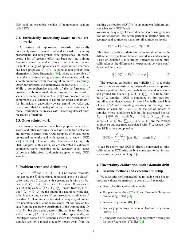
Dependency on magnitude of domain drift We next fo-cused on the Imagenet to assess how calibration depends onthe amount of domain shift. We observe that while stan-dard post-hoc calibrators yield very low in-domain calibra-tion errors ((Fig. 7, ECE at epsilon 0), predictions become

6

CIFAR

0.2

0.4

0.6

0.8

1.0

co

nfi

de

nce

sco

res

Base

TS

TS-P

ETS

ETS-P

TS-IR

TS-IR-P

IR

IR-P

IRM

IRM-P

(a) OOD predictions CIFAR

ObjectNet -OOD

0.0

0.2

0.4

0.6

0.8

1.0

co

nfi

de

nce

sco

res

Base

TS

TS-P

ETS

ETS-P

TS-IR

TS-IR-P

IR

IR-P

IRM

IRM-P

(b) OOD predictions Imagenet (Resnet50).

Figure 6: Distribution of confidence scores for out-of-domain predictions. (a) Confidence scores for our tuning strategy (-P)are substantially lower for the highest perturbation level compared to standard tuning, reflecting that our approach yields wellcalibrated predictions also for truly OOD samples (b) Confidence scores for OOD dataset Objecnet (non-overlapping classes)reveals that our approach results in substantially more uncertainty aware predictions.

increasingly overconfident with increasing domain shift. Incontrast, all methods tuned using our approach had a lowcalibration error for large domain shifts. Notably, we ob-served two types of behaviour for in-domain calibration andsmall domain shift. One set of methods - TS-P, ETS-P andTS-IR-P - had a substantially increased calibration error forin-domain settings compared to standard calibration meth-ods TS, ETS and TS-IR respectively. For these methodsECE at low levels of domain shift was comparable to thatof uncalibrated models, and decreased substantially withdomain shift (in contrast to uncalibrated models or stan-dard calibrators where ECE increases with domain shift).However, IR-P did not show a worse in-domain calibrationcompared to standard post-hoc calibrators when tuned us-ing our approach. Notably, it yielded a calibration errorcomparable to state-of-the-art calibrators for in-domain set-tings, while substantially improving calibration for increas-ing levels of domain shift. We further observed that IRM-P,an accuracy preserving version of IR-P, had a small but con-sistently worse in-domain classification error than IR-P, butperformed substantially better than TS-based methods forsmall domain shifts.One key difference between IR and TS-based methods, isthat the latter methods are accuracy preserving, while IR-P (and IR) can potentially change the ranking of predic-tions and thus accuracy. However, for Imagenet we onlyobserved minor changes in accuracy for IR-based methods,irrespective of tuning strategy (Fig. 4 (b), Fig. 7 (b)). Wehypothesize that the systematic difference in calibration be-haviour is due to the limitations of expressive power of TS-based accuracy-preserving methods: first, by definition theranking between classes in a multi-class prediction does notchange after applying this family of calibrators and secondonly one parameter (for TS) or 4 parameters (ETS) have

to capture the potentially complex behaviour of the calibra-tor. While this has important advantages for practitioners, itcan also result in a lack of expressive power which may beneeded to achieve calibration for all levels of domain drift,ranging from in-domain to truly out-of-domain. Finally, weobserved that a variance reduction via temperature scaling[9] before IR (TS-IR) was also not beneficial for calibrationunder small levels of domain shift.

5.3. Out-of-distribution scenarios

To further investigate the behaviour of post-hoc calibra-tors for truly OOD scenarios, we analysed the distributionof confidence scores for a completely OOD dataset for Im-agenet, using the 200 non-overlapping classes in Objectnet.This revealed that all post-hoc calibrators resulted in signif-icantly less overconfident predictions when tuned using ourapproach. We observed a similar behaviour for CIFAR-10with VGG19, when assessing the distribution of confidencescores at the highest perturbation level across all perturba-tions (Fig. 6).

6. Discussion and conclusion

We present a simple and versatile approach for tuningpost-hoc uncertainty calibration methods. We demonstratethat our new approach, when used in conjunction withisotonic regression-based methods (IR or IRM), yieldswell-calibrated predictions in the case of any level ofdomain drift, from in-domain to truly out-of-domainscenarios. Notably, IR-P and IRM-P maintain their cali-bration performance for in-domain scenarios compared tostandard isotonic regression (IR and IRM). In other words,our experiments suggest that when using our IR(M)-Papproach, there is only a minor trade-off between choos-

7

0 1 2 3 4 5Epsilon

0.00

0.05

0.10

0.15

0.20

0.25

0.30

0.35ECE

(a) ECE Imagenet

0 1 2 3 4 5Epsilon

0.2

0.4

0.6

Accuracy

(b) Accuracy Imagenet

Figure 7: Dependency of accuracy and and ECE on level of domain shift. Accuracy decreases for all methods with increasinglevels of domain shift. For standard post-hoc calibrators ECE also increases, but our approach of tuning on a perturbedvalidation set results in good calibration throughout all levels, especially for IR-P.

ing a model that is either well calibrated in-domain vs.out-of-domain. In contrast, methods based on temperaturescaling may not have enough expressive power to achievegood calibration across this range: standard tuning resultsin highly overconfident OOD predictions and perturbation-based tuning results in calibration errors comparable touncalibrated models for in-domain predictions. However,when averaging across all domain drift scenarios, overallcalibration for TS-P and ETS-P still improves substantiallyover standard TS and ETS. Consequently, for use-casesrequiring an accuracy preserving method and reliableuncertainty estimates especially for larger levels of domainshift, TS-P and ETS-P are good options.We further observe this trade-off between accuracy preserv-ing properties and calibration error for IR-based methods.While IRM-P has accuracy-preserving properties, overallcalibration errors are higher than for IR-P in particular forsmall domain shifts.

Our perturbation-based tuning can be readily applied toany post-hoc calibration method. When used in combina-tion with an expressive non-parametric method such as IR,this results in well calibrated predictions not only for in-domain and small domain shifts, but also for truly OODsamples. This is in stark contrast to existing methods withstandard tuning, where performance in terms of calibra-tion and uncertainty-awareness degrades with increasingdomain drift.

7. Acknowledgements

This work was supported by the Munich Center for Ma-chine Learning and has been funded by the German FederalMinistry of Education and Research (BMBF) under GrantNo. 01IS18036B.

8

References[1] Andrei Barbu, David Mayo, Julian Alverio, William Luo,

Christopher Wang, Dan Gutfreund, Josh Tenenbaum, andBoris Katz. Objectnet: A large-scale bias-controlled datasetfor pushing the limits of object recognition models. InAdvances in Neural Information Processing Systems, pages9448–9458, 2019. 1, 4

[2] Francois Chollet. Xception: Deep learning with depthwiseseparable convolutions. In Proceedings of the IEEE con-ference on computer vision and pattern recognition, pages1251–1258, 2017. 5

[3] Yarin Gal and Zoubin Ghahramani. Dropout as a bayesianapproximation: Representing model uncertainty in deeplearning. In international conference on machine learning,pages 1050–1059, 2016. 3

[4] Chuan Guo, Geoff Pleiss, Yu Sun, and Kilian Q. Weinberger.On calibration of modern neural networks. In Proceedingsof the 34th International Conference on Machine Learning-Volume 70, pages 1321–1330. JMLR. org, 2017. 1, 2, 3

[5] Kaiming He, Xiangyu Zhang, Shaoqing Ren, and Jian Sun.Deep residual learning for image recognition. In Proceed-ings of the IEEE conference on computer vision and patternrecognition, pages 770–778, 2016. 5

[6] Dan Hendrycks and Thomas Dietterich. Benchmarking neu-ral network robustness to common corruptions and perturba-tions. arXiv preprint arXiv:1903.12261, 2019. 4, 5, 10, 15

[7] Gao Huang, Zhuang Liu, Laurens Van Der Maaten, and Kil-ian Q Weinberger. Densely connected convolutional net-works. In Proceedings of the IEEE conference on computervision and pattern recognition, pages 4700–4708, 2017. 5

[8] Heinrich Jiang, Been Kim, Melody Guan, and Maya Gupta.To trust or not to trust a classifier. In Advances in NeuralInformation Processing Systems, pages 5541–5552, 2018. 3

[9] Ananya Kumar, Percy S Liang, and Tengyu Ma. Verifieduncertainty calibration. In Advances in Neural InformationProcessing Systems, pages 3792–3803, 2019. 7, 11

[10] Balaji Lakshminarayanan, Alexander Pritzel, and CharlesBlundell. Simple and scalable predictive uncertainty esti-mation using deep ensembles. In Advances in Neural Infor-mation Processing Systems, pages 6402–6413, 2017. 3

[11] Shiyu Liang, Yixuan Li, and R. Srikant. Enhancing the re-liability of out-of-distribution image detection in neural net-works. 2018. 3

[12] Mahdi Pakdaman Naeini, Gregory Cooper, and MilosHauskrecht. Obtaining well calibrated probabilities usingbayesian binning. In Twenty-Ninth AAAI Conference on Ar-tificial Intelligence, 2015. 2, 3

[13] Yaniv Ovadia, Emily Fertig, Jie Ren, Zachary Nado, DavidSculley, Sebastian Nowozin, Joshua Dillon, Balaji Lakshmi-narayanan, and Jasper Snoek. Can you trust your model’suncertainty? evaluating predictive uncertainty under datasetshift. In Advances in Neural Information Processing Sys-tems, pages 13991–14002, 2019. 3

[14] Nicolas Papernot and Patrick McDaniel. Deep k-nearestneighbors: Towards confident, interpretable and robust deeplearning. arXiv preprint arXiv:1803.04765, 2018. 3

[15] John C. Platt. Probabilistic outputs for support vector ma-chines and comparisons to regularized likelihood methods.In Advances in large margin classifiers, pages 61–74. MITPress, 1999. 1, 2, 11

[16] Mark Sandler, Andrew Howard, Menglong Zhu, Andrey Zh-moginov, and Liang-Chieh Chen. Mobilenetv2: Invertedresiduals and linear bottlenecks. In Proceedings of theIEEE conference on computer vision and pattern recogni-tion, pages 4510–4520, 2018. 5

[17] Murat Sensoy, Lance Kaplan, and Melih Kandemir. Eviden-tial deep learning to quantify classification uncertainty. InAdvances in Neural Information Processing Systems, pages3179–3189, 2018. 3

[18] Karen Simonyan and Andrew Zisserman. Very deep convo-lutional networks for large-scale image recognition. arXivpreprint arXiv:1409.1556, 2014. 5

[19] Mingxing Tan and Quoc V Le. Efficientnet: Rethinkingmodel scaling for convolutional neural networks. arXivpreprint arXiv:1905.11946, 2019. 5

[20] Christian Tomani and Florian Buettner. Towards trustworthypredictions from deep neural networks with fast adversarialcalibration. In Thirty-Fifth AAAI Conference on ArtificialIntelligence, 2021. 3

[21] Yeming Wen, Paul Vicol, Jimmy Ba, Dustin Tran, andRoger Grosse. Flipout: Efficient pseudo-independentweight perturbations on mini-batches. arXiv preprintarXiv:1803.04386, 2018. 3

[22] Bianca Zadrozny and Charles Elkan. Obtaining calibratedprobability estimates from decision trees and naive bayesianclassifiers. In Icml, volume 1, pages 609–616. Citeseer,2001. 1, 2, 11

[23] Bianca Zadrozny and Charles Elkan. Transforming classifierscores into accurate multiclass probability estimates. In Pro-ceedings of the eighth ACM SIGKDD international confer-ence on Knowledge discovery and data mining, pages 694–699, 2002. 1, 2, 3

[24] Jize Zhang, Bhavya Kailkhura, and T Han. Mix-n-match:Ensemble and compositional methods for uncertainty cal-ibration in deep learning. In International Conference onMachine Learning (ICML), 2020. 1, 2, 3

9

A. Appendix SummaryWe provide further details on the implementation of our algorithm as well as additional results. This appendix is structured

as follows.

• In section B, we first formalize our algorithm in Algorithm 1. We then provide more details on the test perturbationsused for our analyses, along with their parameter sets.

• In section C, we report supplementary results, including additional metrics as well as data on additional baselines andadditional experiments on the robustness of our findings.

• In section D, we consolidate our results into a brief recommendation for practitioners.

B. Additional implementation detailsB.1. Algorithm

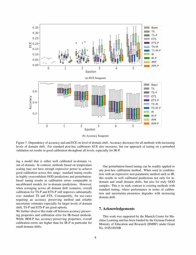
Algorithm 1 Tuning of a post-calibration method for domain shift scenariosInput: Classification model Y = f(X), validation set (X,Y ), number of perturbation levels N , number of classes C, initialparameter εinit.

1: Compute min and max accuracy: accmin = 1/C; accmax = acc(f(X), Y )2: Compute N evenly spaced accuracy levels A = {accmin, accmin + accmax−accmin

N−1 , . . . , accmax}3: Initialise empty perturbed validation set (XE , YE)4: for i in 1:N do5: if i = 1 then6: Set εi = εinit7: end if8: Compute Xεi = X +N (0, εi), by drawing a sample from a Gaussian N (0, εi) with variance εi for every pixel (j, k)

in every image xj,k ∈ X9: Minimize acc(f(Xεi), Y )−Ai with respect to εi, using a Nelder-Mead optimizer

10: Compute Xεi = X +N (0, εi) using optimized εi11: Add (Xεi , Y ) to (XE , YE)12: if i < N then13: Initialise εi+1 = εi14: end if15: end for16: Tune post-processing method on (XE , YE)

B.2. Perturbation strategies

For the affine test perturbation strategies (Table 2) we chose 10 levels of perturbation with increasing perturbation strengthuntil random levels of accuracy were reached (or parameters could not be increased any further). We started all test perturba-tion sequences at no perturbation and list specific levels of perturbation in Table 2.For Imagenet corruptions, we follow [6] and report test accuracy as well as accuracy under maximum domain shift in Table3.

10

C. Additional resultsC.1. Additional baselines

In addition to the state-of-the-art post-calibrators analysed in detail in the main paper, we also assessed the effect of tuningbased on a perturbed validation set for additional baselines. Here, we report results for CIFAR-10 for Platt scaling [15],histogram binning [22] and a recently proposed approach combining Platt scaling with histogram binning (PBMC) [9].Table 4 reveals that also these baselines benefit from tuning on a perturbed validation set; note however that overall ECE wasconsistently higher for these baselines compared to IR-P, for all architectures.

C.2. Additional metrics

In addition to the expected calibration error as reported in the main paper, we also compute a debiased ECE, recentlyproposed in [9], that can be more robust than the standard definition of ECE. Also with this measure, our approach improvesall baselines consistently, with IRM-P, IR-P and TS-IR-P performing best (Table 5).

Table 2: For rotation, perturbation is the (left or right) rotation angle in degrees, shift is measured in pixels in x or y direction,for shear the perturbation is measured as shear angle in counter-clockwise direction in degrees, for zoom the perturbation iszoom in x or y direction.

Perurbation Perturbation-specific parameter

rot left 0 350 340 330 320 310 300 290 280 270rot right 0 10 20 30 40 50 60 70 80 90shear 0 10 20 30 40 50 60 70 80 90xyshift 0 2 4 6 8 10 12 14 16 18xshift 0 2 4 6 8 10 12 14 16 18xyshift 0 2 4 6 8 10 12 14 16 18xyzoom 1 0.90 0.80 0.70 0.60 0.50 0.40 0.30 0.20 0.10xzoom 1 0.90 0.80 0.70 0.60 0.50 0.40 0.30 0.20 0.10yzoom 1 0.90 0.80 0.70 0.60 0.50 0.40 0.30 0.20 0.10

Table 3: Accuracies for Imagenet perturbations in-domain and with maximum shift.

Perurbation AccuracyIn-Domain Max Domain-Shift

shot noise 0.7452 0.07752impulse noise 0.7452 0.07104defocus blur 0.7452 0.14784glass blur 0.7452 0.06904motion blur 0.7452 0.09696zoom blur 0.7452 0.22864snow 0.7452 0.17776frost 0.7452 0.25016fog 0.7452 0.40912brightness 0.7452 0.56776contrast 0.7452 0.06416elastic transform 0.7452 0.14480pixelate 0.7452 0.19216jpeg compression 0.7452 0.41136gaussian blur 0.7452 0.10016saturate 0.7452 0.47952spatter 0.7452 0.30808speckle noise 0.7452 0.18296

11

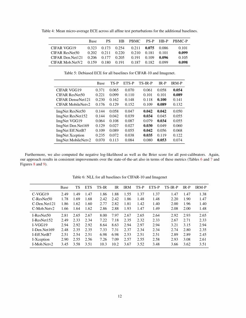
Table 4: Mean micro-average ECE across all affine test perturbations for the additional baselines.

Base PS HB PBMC PS-P HB-P PBMC-P

CIFAR VGG19 0.323 0.173 0.254 0.211 0.075 0.086 0.101CIFAR ResNet50 0.202 0.211 0.220 0.210 0.181 0.101 0.099CIFAR Den.Net121 0.206 0.177 0.205 0.191 0.109 0.096 0.105CIFAR Mob.NetV2 0.159 0.180 0.191 0.187 0.182 0.099 0.098

Table 5: Debiased ECE for all baselines for CIFAR-10 and Imagenet.

Base TS-P ETS-P TS-IR-P IR-P IRM-P

CIFAR VGG19 0.371 0.065 0.070 0.061 0.058 0.054CIFAR ResNet50 0.221 0.099 0.110 0.101 0.101 0.089CIFAR DenseNet121 0.230 0.162 0.148 0.118 0.100 0.141CIFAR MobileNetv2 0.176 0.129 0.152 0.109 0.089 0.132

ImgNet ResNet50 0.144 0.058 0.047 0.042 0.042 0.050ImgNet ResNet152 0.144 0.042 0.039 0.034 0.045 0.055ImgNet VGG19 0.064 0.108 0.087 0.079 0.034 0.055ImgNet Den.Net169 0.129 0.027 0.027 0.030 0.049 0.060ImgNet Eff.NetB7 0.109 0.089 0.055 0.042 0.056 0.068ImgNet Xception 0.235 0.072 0.038 0.035 0.119 0.122ImgNet MobileNetv2 0.070 0.113 0.084 0.080 0.053 0.074

Furthermore, we also computed the negative log-likelihood as well as the Brier score for all post-calibrators. Again,our approach results in consistent improvements over the state-of-the-art also in terms of these metrics (Tables 6 and 7 andFigures 8 and 9).

Table 6: NLL for all baselines for CIFAR-10 and Imagenet

Base TS ETS TS-IR IR IRM TS-P ETS-P TS-IR-P IR-P IRM-P

C-VGG19 2.49 1.49 1.47 1.86 1.88 1.55 1.37 1.37 1.47 1.47 1.38C-ResNet50 1.78 1.69 1.68 2.42 2.42 1.86 1.48 1.48 2.20 1.90 1.47C-Den.Net121 1.86 1.62 1.60 2.77 2.82 1.81 1.42 1.40 2.00 1.96 1.40C-Mob.Netv2 1.66 1.64 1.62 2.86 2.88 1.93 1.47 1.49 2.08 2.00 1.48

I-ResNet50 2.81 2.65 2.67 8.00 7.97 2.67 2.65 2.64 2.92 2.93 2.65I-ResNet152 2.49 2.33 2.34 7.22 7.18 2.35 2.32 2.33 2.67 2.71 2.33I-VGG19 2.94 2.92 2.92 8.64 8.63 2.94 2.97 2.94 3.21 3.15 2.94I-Den.Net169 2.48 2.35 2.35 7.33 7.31 2.37 2.34 2.34 2.74 2.80 2.35I-Eff.NetB7 2.51 2.54 2.51 6.98 6.98 2.53 2.51 2.51 2.89 2.89 2.45I-Xception 2.90 2.55 2.56 7.26 7.09 2.57 2.55 2.58 2.93 3.08 2.61I-Mob.Netv2 3.45 3.58 3.51 10.3 10.2 3.67 3.52 3.48 3.66 3.62 3.51

12

Table 7: Brier score for all baselines for CIFAR-10 and Imagenet

Base TS ETS TS-IR IR IRM TS-P ETS-P TS-IR-P IR-P IRM-P

C-VGG19 .731 .603 .600 .617 .620 .610 .565 .566 .574 .574 .566C-ResNet50 .677 .663 .660 .681 .681 .664 .622 .624 .664 .659 .620C-Den.Net121 .631 .600 .598 .618 .618 .601 .593 .587 .623 .607 .584C-Mob.NetV2 .644 .640 .636 .656 .656 .639 .619 .627 .655 .642 .621

I-ResNet50 .667 .644 .648 .692 .692 .649 .646 .644 .645 .643 .644I-ResNet152 .620 .597 .598 .645 .643 .600 .597 .596 .597 .597 .598I-VGG19 .688 .686 .687 .732 .732 .687 .699 .694 .691 .681 .688I-Den.Net169 .620 .602 .602 .650 .650 .604 .600 .600 .595 .596 .603I-Eff.NetB7 .621 .634 .619 .635 .635 .608 .617 .612 .584 .586 .608I-Xception .682 .625 .621 .657 .661 .627 .624 .620 .611 .627 .635I-Mob.NetV2 .745 .767 .758 .803 .802 .754 .759 .751 .740 .734 .750

0 1 2 3 4 5Epsilon

0.4

0.6

0.8

1.0

1.2

bri

er

score

Figure 8: Brier score for Resnet50 trained on Imagenet

0 1 2 3 4 5Epsilon

5

10

15

20

NLL

Figure 9: NLL for Resnet50 trained on Imagenet

To further illustrate the benefit of our modelling approach for different post-calibration methods, we computed for eachalgorithm the difference in mean ECE between our approach (using a perturbed validation set) and the standard approach(using the unperturbed validation set). Table 8 highlights that our approach is beneficial for all post-calibration algorithms.

13

Table 8: ∆ECE reveals that using a perturbed validation set for training improves performance across all methods for CIFAR-10 (higher is better).

∆ TS ∆ ETS ∆ TS-IR ∆ IR ∆ IRM

CIFAR VGG19 0.661 0.622 0.706 0.718 0.736CIFAR ResNet50 0.528 0.473 0.518 0.509 0.575CIFAR DenseNet121 0.103 0.158 0.376 0.472 0.208CIFAR MobileNetv2 0.281 0.113 0.428 0.519 0.266

ImgNet ResNet50 -0.022 0.365 0.753 0.740 0.428ImgNet ResNet152 0.147 0.301 0.778 0.708 0.276ImgNet VGG19 -1.044 -0.567 0.467 0.762 0.085ImgNet Den.Net169 0.453 0.421 0.795 0.662 0.118ImgNet Eff.NetB7 0.451 0.440 0.705 0.622 0.218ImgNet Xception 0.110 0.253 0.715 0.221 -0.313ImgNet MobileNetv2 0.304 0.348 0.644 0.745 0.356

C.3. Additional experiments

Size of validation set While both IRM-P and IR-P performed consistently well across baselines, a key difference is thatIR-P is not accuracy preserving. In contrast, a model’s accuracy remains unchanged after post-calibration with IRM-P. Inthe main paper, we show that the effect on the accuracy for IR-P is only marginal. To further investigate the robustness ofIR-P in terms of accuracy, we assessed the effect of the size of the validation set on performance. Our results show, that infact for small validation sets accuracy can substantially decrease for IR-P (Fig. 10 (b)). However, with increasing size ofthe validation set accuracy increases and ECE decreases (Fig. 10 (a)). This suggests that for sufficiently large validation set,IR-based methods benefit from their high expressiveness.

0 1000 2000 3000 4000 5000

Validat ion Set Size

0.045

0.050

0.055

0.060

0.065

0.070

Me

an

EC

E S

co

re

TS-IR-P

IR-P

IRM-P

(a) Mean ECE w.r.t. size of validation set

0 1000 2000 3000 4000 5000Validation Set Size

0.850

0.852

0.854

0.856

0.858

0.860

Accu

racy

TS-IR-PIR-PIRM-P

(b) Accuracy w.r.t. size of validation set

Figure 10: Effect of the chosen size of the validation set on the mean expected calibration error and accuracy scores (CIFAR-10).

14

Base TS ETS TS-IR IR IRM TS-H ETS-H TS-IR-H IR-H IRM-H

0.323 0.158 0.152 0.173 0.176 0.167 0.102 0.096 0.112 0.127 0.114

Table 9: Mean expected calibration error across all test domain drift scenarios (affine transformations for CIFAR-10). Tuningwas performed on the validation set and the perturbed validation set generated by applying the validation perturbationsproposed in [6]. The latter is denoted by the suffix -H.

Type of validation perturbation Finally, we investigated the effect of the perturbation strategy used to generate a perturbedvalidation set. To this end, we assessed whether perturbing the validation set using image perturbations rather than the genericperturbations proposed in our work, could lead to similar results. To test this hypothesis, we used the validation perturbationsspeckle noise, gaussian blur, spatter and saturate introduced in [6] to generate a perturbed validation set. We then tuned allbaselines on this validation set using a VGG19 model trained on CIFAR-10. Table 9 shows that this resulted in consistentlyworse calibration errors compared to the generic perturbation strategy proposed in the main paper. This suggests, that ouralgorithm can indeed yield a validation set that is representative of generic domain drift scenarios.

D. Additional GuidelinesBased on our extensive experiments, we propose the following guidelines for practitioners:

• If a sufficiently large validation set is available and calibration for in-domain settings is of particular concern, werecommend using IR-P or TS-IR-P. This may result in changes in model accuracy.

• If the practitioner requires that the accuracy of the trained model remains unchanged or truly OOD scenarios are ofparticular concern, we recommend using IRM-P or ETS-P.

15