geotechnical properties of the travis peak (hosston
TRANSCRIPT

Stephen F. Austin State University Stephen F. Austin State University
SFA ScholarWorks SFA ScholarWorks
Electronic Theses and Dissertations
12-2016
Geotechnical Properties Of the Travis Peak (Hosston) Formation Geotechnical Properties Of the Travis Peak (Hosston) Formation
in East Texas: A Compressive and Tensile Strength Analysis using in East Texas: A Compressive and Tensile Strength Analysis using
Regression Analysis. Regression Analysis.
Pawan Kakarla Stephen F Austin State University, [email protected]
Follow this and additional works at: https://scholarworks.sfasu.edu/etds
Part of the Geology Commons, and the Geotechnical Engineering Commons
Tell us how this article helped you.
Repository Citation Repository Citation Kakarla, Pawan, "Geotechnical Properties Of the Travis Peak (Hosston) Formation in East Texas: A Compressive and Tensile Strength Analysis using Regression Analysis." (2016). Electronic Theses and Dissertations. 62. https://scholarworks.sfasu.edu/etds/62
This Thesis is brought to you for free and open access by SFA ScholarWorks. It has been accepted for inclusion in Electronic Theses and Dissertations by an authorized administrator of SFA ScholarWorks. For more information, please contact [email protected].

Geotechnical Properties Of the Travis Peak (Hosston) Formation in East Texas: A Geotechnical Properties Of the Travis Peak (Hosston) Formation in East Texas: A Compressive and Tensile Strength Analysis using Regression Analysis. Compressive and Tensile Strength Analysis using Regression Analysis.
Creative Commons License Creative Commons License
This work is licensed under a Creative Commons Attribution-Noncommercial-No Derivative Works 4.0 License.
This thesis is available at SFA ScholarWorks: https://scholarworks.sfasu.edu/etds/62
GEOTECHNICAL PROPERTIES OF THE TRAVIS PEAK (HOSSTON)
FORMATION IN EAST TEXAS: A COMPRESSIVE AND TENSILE
STRENGTH ANALYSIS USING REGRESSION ANALYSIS.
By
PAWAN KAKARLA, Master of
Technology
Presented to the Faculty of the Graduate School of
Stephen F. Austin State University
In Partial Fulfillment
Of the Requirements
For the Degree of
Master of Science
STEPHEN F. AUSTIN STATE UNIVERSITY
December, 2016

GEOTECHNICAL PROPERTIES OF THE TRAVIS PEAK (HOSSTON)
FORMATION IN EAST TEXAS: A COMPRESSIVE AND TENSILE
STRENGTH ANALYSIS USING REGRESSION ANALYSIS.
PAWAN KAKARLA, Master of Technology.
APPROVED:
Dr. Wesley Brown, Thesis Director
Dr. Chris Barker, Committee Member
Dr. R. LaRell Nielson, Committee Member
Dr. Kent Riggs, Committee Member
Richard Berry, D.M.A
Dean of the Graduate School

i
ABSTRACT
The estimation of rock mass strength is a key parameter in geotechnical
engineering which is used in the design of geotechnical structures like tunnels, dams and
slopes. Geotechnical engineering is the branch of civil engineering which works on the
principles of soil and rock mechanics to evaluate subsurface conditions, stability of
slopes, foundations of structures and construction of earthworks. The main focus of this
study was to calculate the strength of Lower Cretaceous Travis Peak Formation rocks of
East Texas and to check the accuracy by comparing it with Regression analysis. The
parameters which were used were the Uniaxial Compression Test (UCS) and tensile
strength.
Core samples were collected at Stephen F. Austin State University Core Lab
Repository. Strength tests were conducted at the lab facilities of University of Houston.
Parameters such as load for UCS and tensile strength were experimentally
determined using procedures outlined by the International Society of Rock Mechanics
(ISRM, Rock characterization testing and monitoring, 1981). In this study, a linear
regression analysis was also performed to predict and compare the strength values of the
core rock samples from the Travis Peak Formation.
Based on previous studies, it was shown that regression analysis is accurate in
providing the strength of rocks. The results obtained from the tests are useful in
predicting the strength of rocks from the Travis Peak Formation.

ii
Uniaxial compression and tensile strength tests were performed for 12 samples at
the Department of Civil Engineering’s Laboratory at the University of Houston. Before
the tests, the samples were cut before into the size of 7.2 to 3.6 in ratio of length to
diameter to maintain a 2:1 ratio.
The average value of UCS for the 12 samples was 27.43 MPa. Similarly, the
average value for tensile strength for 12 samples was 4.05 MPa. Based on the values
which were calculated, these samples were classified as medium strength rocks which
belongs to Class D.
Linear Regression analysis was performed using MATLAB software for
predicting the strength of core rock samples. The equation for linear regression was in the
form of 𝒀𝟏 = 𝟎. 𝟏𝟎𝟎𝟓 ×𝑿𝟏 + (𝟏. 𝟐𝟗𝟑), where y is the tensile strength and x is UCS. The
root mean square generated for regression analysis was 0.6378.

iii
ACKNOWLEDGMENTS
I would like to thank Dr. Cumaraswamy Vipulanandan, Professor at the
Department of Civil and Environmental Engineering, University of Houston for allowing
me to use their laboratory so that I was able to finish my testing on uniaxial compressive
strength and tensile strength. I would especially thank Mr. Anudeep Reddy, graduate
student at the Department of Civil and Environmental Engineering, University of
Houston for assisting me in completion of this work. His assistance in preparing the
samples and using the instrument for testing were invaluable.
I would like to thank Dr. Wesley Brown, my graduate advisor, for allowing me
the freedom to complete this work on my own schedule and for being incredibly patient
and understanding during this process. I would like to thank each member of my final
thesis committee and the support of my family and friends.

iv
TABLE OF CONTENTS
ABSTRACT ......................................................................................................................... i
ACKNOWLEDGMENTS ................................................................................................. iii
LIST OF TABLES ............................................................................................................. ix
LIST OF EQUATIONS ...................................................................................................... x
OBJECTIVE ....................................................................................................................... 1
INTRODUCTION .............................................................................................................. 2
REGIONAL SETTING ...................................................................................................... 4
STRATIGRAPHIC SETTING ......................................................................................... 14
UNIAXIAL COMPRESSIVE TEST ................................................................................ 24
Point load test to determine compressive strength .........................................................28
Point load strength index (Is) ..................................................................................... 28
Correlation between point load strength and uniaxial compressive strength ............ 29
Compressive strength from Schmidt Hammer test ........................................................30
TENSILE STRENGTH .................................................................................................... 36
Splitting Tensile Test .....................................................................................................36
Flexure Test ....................................................................................................................40
Regression Analysis .......................................................................................................46

v
Independent variables and Dependent variables ............................................................49
RESULTS ......................................................................................................................... 52
Uniaxial Compressive Strength ......................................................................................52
Tensile Strength..............................................................................................................57
Regression Analysis .......................................................................................................62
Uniaxial Compressive Strength vs Tensile Strength ................................................. 62
Box Plots ........................................................................................................................64
DISCUSSION ................................................................................................................... 67
CONCLUSIONS............................................................................................................... 68
FUTURE WORK .............................................................................................................. 70
REFERENCES ................................................................................................................. 71
APPENDIX A – CORE SAMPLES DATABASE ........................................................... 78
APPENDIX B – HAND SAMPLE DESCRIPTIONS...................................................... 81
VITA ................................................................................................................................. 90

vi
LIST OF FIGURES
Figure 1 – Gulf of Mexico’s geologic framework showing crustal types ( T. C. -
Transitional continental crust; O. C. – Oceanic Crust) and depth to the top of the
basement (Galloway, 2009). ............................................................................................... 6
Figure 2 - Map showing the tectonic setting of the East Texas Basin, adapted from
(Martin, 1978) ..................................................................................................................... 7
Figure 3 – Map showing the location of the East Texas basin, Houston embayment,
Brazos basin and the other structural features of east Texas (Davidoff, 1991). ................. 8
Figure 4 – Structural cross sections across the East Texas Basin (Wood & Guevara,
1981). ................................................................................................................................ 10
Figure 5 – Map area showing East Texas counties and the location of wells
that were used in this study. The samples are taken from the highlighted counties. ........ 11
Figure 6 – Stratigraphic column of the East Texas basin; highlighted portion
showing the Travis Peak Formation (modified from (Arkansas Geological Survey,
2016)). ............................................................................................................................... 15
Figure 7 - Structure, top of the Cotton Valley Group Sandstone (base of Travis Peak
Formation), showing the location of this study (modified from (Finley, 1984)). ............. 16
Figure 8 – Image showing the arrangement of Unconfined Compression test
which can hold up to a core sample of NX size and in the center is the sample
taken from a core which has a length to diameter ratio of 2 (Geocomp Corp, 2015). ...... 27
vii
Figure 9 – L type Schmidt Hammer, where A is the needle which is placed at
the surface of the rock and B is the scale of the hammer which is used to measure
the strength in MPa (Proceq, 2016). ................................................................................. 31
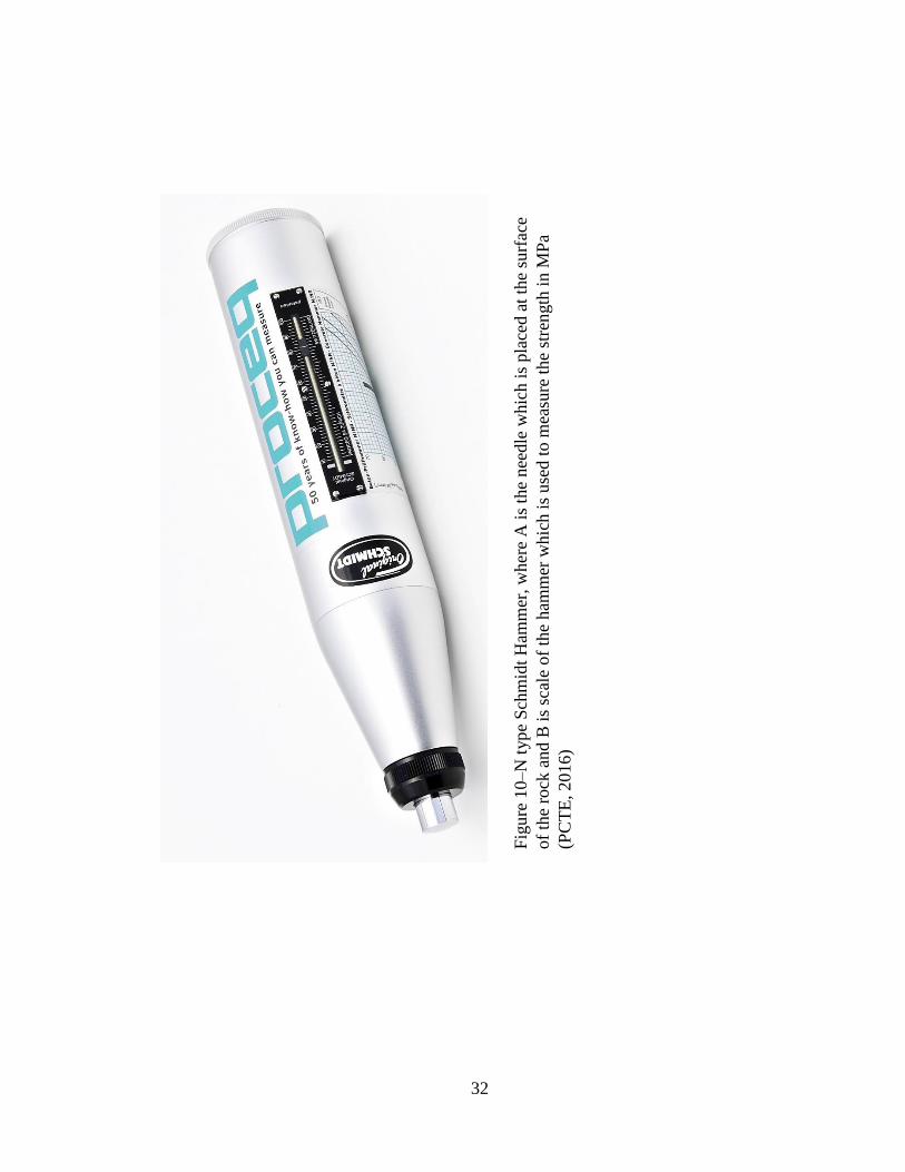
Figure 10 – N type Schmidt Hammer, where A is the needle which is placed at
the surface of the rock and B is scale of the hammer which is used to measure the
strength in MPa (PCTE, 2016).......................................................................................... 32
Figure 11 – Image showing the arrangement of Tensile strength, which can also
hold up a core size of NX size, and a length to diameter ratio of 4 or 5 (Istone, n.d.) ..... 38
Figure 12 – Horizontal and Vertical stresses measured from Splitting tensile test
(Building Research Institute, 2016). ................................................................................. 39
Figure 13 – Image showing a core rock sample which was tested for UCS and
Tensile strength which was cut into dimensions of 3.6 in width and 7.2 in length. ......... 44
Figure 14 – Equipment used for testing the compressive strength and tensile
strength at University of Houston’s Civil Engineering Laboratory. The same
equipment is used to test the UCS and Tensile strength and the samples are
rested on the instrument depending upon the test and the load is applied. ....................... 45
Figure 15–Image showing the equation for the linear regression analysis and
the trendline (University of Washington, 2016). .............................................................. 48
Figure 16–The above figure shows three different types of linear regression
equations. First image shows a positive trend of the linear equation which has

viii
a positive slope. Second one shows a negative trend of the linear equation which
has a negative slope. Third one is a non-linear equation (Laerd Statistics, 2016). ........... 48
Figure 17 – Top and bottom of the samples are flattened by adding Sulfur which
is melted at 300° F. ........................................................................................................... 54
Figure 18 – Failure from the maximum stress plane (σ1) results in the uniaxial
compressive strength test. ................................................................................................. 55
Figure 19–A plot showing the frequency histogram for UCS with the maximum
number of 6 samples lie in the range of 28.23 to 43.23 MPa and minimum number
of 1 sample lying in the range of 43.23 to 58.23 MPa. ..................................................... 58
Figure 20 - Failure from minimum stress plane (σ3) results in tensile strength................ 59
Figure 21–A plot showing the frequency histogram for Tensile strength, where
the maximum number of 6 samples lying in the range of 3.59 to 5.49 MPa and a
minimum of 2 samples lying in the range of 5.49 to 7.39 MPa. ....................................... 61
Figure 22 – A plot showing linear regression analysis between Uniaxial
Compressive Strength and Tensile strength which has a R-square value of 0.6378. ....... 63
Figure 23 – Box plot showing the difference in the values between UCS and
Tensile strength. The y–axis is strength in MPa. .............................................................. 65

ix
LIST OF TABLES
Table 1 – Various strength classification of intact rock (Bieniawski, 1984). ................... 26
Table 3 – Various classifications of point load strength index (Is) after (Bieniawski,
1984). ................................................................................................................................ 28
Table 4 – Various classification of k after (Palmstrom, 2011), where D is diameter. ...... 29
Table 5 – Compressive Strength of rocks from field identification (ISRM, 1978) .......... 34
Table 6 – Strength classification of intact and jointed rocks (Ramamurthy & Arora,
1993). ................................................................................................................................ 43
Table 7–Table showing the data generated from the laboratory equipment for UCS
and Tensile strength. ......................................................................................................... 66
Table 8 - Table showing details on the core samples that must be used for the testing. .. 78
x
LIST OF EQUATIONS
(1) σc = k × Is ……………………………………………………………………….29
(2) fbt = Pl ÷ bd2 ………………………………………………………………….......40
(3) y = βx + ε…………………………………………………………………………..49
(4) UCS (lbfin2) = Load (P in lbf)Area (inches2)……………………………….........53
(5) T = 2PπDL ………………………………………………………………………….57
(6) Y1 = 0.1005 ×X1 + (1.293) ……………………………………………………..62
1
OBJECTIVE
The objectives of this study are to calculate uniaxial compressive strength and
tensile strength of rocks in core samples from the Travis Peak Formation in East Texas
and then predict the values using Linear Regression Analysis. These objectives are
accomplished by using following methods:
1. Measuring the load for uniaxial compressive strength and tensile strength tests.
2. Calculating the uniaxial compressive strength and tensile strength using the
measured load.
3. Predicting the strength values for rock samples from the Travis Peak Formation
using linear regression analysis.

2
INTRODUCTION
The most widely used techniques to determine the strength of rock masses are the
uniaxial compressive strength (UCS) and tensile strength tests (Çanakçi, Baykasoǧlu, &
Güllü, 2009). Uniaxial compressive strength is a compressive strength of the material to
withstand loads which has a tendency to reduce the size. UCS is the test which can resist
compression. Similarly, Tensile strength is the strength of a material which can withstand
loads and has a tendency to elongate. Tensile strength can resist tension. There are two
ways to approach this. Firstly, there is the direct approach which involves collecting and
testing the specimens in the laboratory. Secondly, there is the indirect approach which is
to make use of previously determined empirical equations from the literature
(Baykasoǧlu, Güllü, Çanakçi, & Özbakir, 2008). A standard procedure for this testing
was followed based on (ASTM D 2938-95), (ASTM D 3967-95a) and (ISRM, Rock
characterization testing and monitoring, 1981). The acronym ASTM stands for the
American Society of the International Association for Testing and Materials. It develops
and publishes standards for testing of various materials and products. ISRM stands for the
International Society for Rock Mechanics. The major function of ISRM is to publish
standards for all tests that are used in studies related to rock mechanics, civil engineering,
mining and petroleum engineering. In this study, all the tests are conducted based on the
standards set by the ISRM.
Experimental tests for measuring UCS and tensile strength are preferred for
designs and modeling. However, indirect methods are quite frequently used because they
are simpler, faster and economical, particularly under limited laboratory testing

3
conditions (Çanakçi, Baykasoǧlu, & Güllü, 2009). Indirect methods include simple index
test variables such as impact strength and point load index to estimate UCS (Fener,
Kahraman, Bilgil, & Gunaydin, 2005). Empirical equations are also used to calculate
tensile strength.
The main aim was to calculate the uniaxial compressive strength and tensile
strength of the core rock samples from the laboratory methods. Based on the calculations,
linear regression analysis was used to predicting the strength of the core rock samples.
The input variables that were used are UCS load, tensile strength load and area. UCS and
tensile strength are the parameters that were predicted, thus they are the output variables.
4
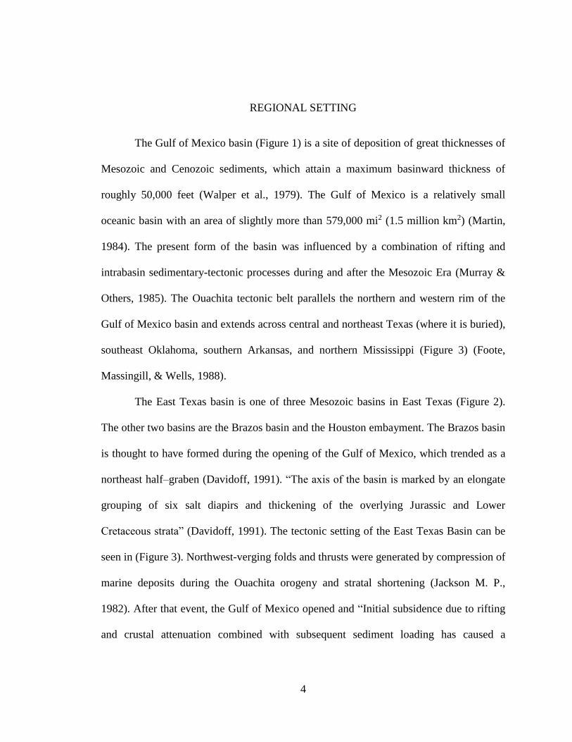
REGIONAL SETTING
The Gulf of Mexico basin (Figure 1) is a site of deposition of great thicknesses of
Mesozoic and Cenozoic sediments, which attain a maximum basinward thickness of
roughly 50,000 feet (Walper et al., 1979). The Gulf of Mexico is a relatively small
oceanic basin with an area of slightly more than 579,000 mi2 (1.5 million km2) (Martin,
1984). The present form of the basin was influenced by a combination of rifting and
intrabasin sedimentary-tectonic processes during and after the Mesozoic Era (Murray &
Others, 1985). The Ouachita tectonic belt parallels the northern and western rim of the
Gulf of Mexico basin and extends across central and northeast Texas (where it is buried),
southeast Oklahoma, southern Arkansas, and northern Mississippi (Figure 3) (Foote,
Massingill, & Wells, 1988).
The East Texas basin is one of three Mesozoic basins in East Texas (Figure 2).
The other two basins are the Brazos basin and the Houston embayment. The Brazos basin
is thought to have formed during the opening of the Gulf of Mexico, which trended as a
northeast half–graben (Davidoff, 1991). “The axis of the basin is marked by an elongate
grouping of six salt diapirs and thickening of the overlying Jurassic and Lower
Cretaceous strata” (Davidoff, 1991). The tectonic setting of the East Texas Basin can be
seen in (Figure 3). Northwest-verging folds and thrusts were generated by compression of
marine deposits during the Ouachita orogeny and stratal shortening (Jackson M. P.,
1982). After that event, the Gulf of Mexico opened and “Initial subsidence due to rifting
and crustal attenuation combined with subsequent sediment loading has caused a

5
maximum subsidence of more than 23,000 ft (7,010 m) in the center of the basin”
(Jackson & Seni, 1984).

6
Figure 1–Gulf of Mexico’s geologic framework showing crustal types ( T. C. -
Transitional continental crust; O. C. – Oceanic Crust) and depth to the top of the
basement (Galloway, 2009).

7
Figure 2–Map showing the tectonic setting of the East Texas Basin, adapted from
(Martin, 1978)

8
Figure 3–Map showing the location of the East Texas basin, Houston embayment, Brazos
basin and the other structural features of east Texas (Davidoff, 1991).

9
As the Gulf of Mexico basin periodically filled with sea water, the evaporitic
Louann Salt was deposited on an eroded post-rift, pre-breakup terrane which was due to
the further subsidence of the marine incursions (Jackson M. P., 1982). “From (Figure 3)
the updip limit of the Louann Salt is parallel to the Ouachita trends, because the Ouachita
area during the Jurassic was still at some elevation as compared to subsiding East Texas
Basin” (Jackson M. P., 1982). A monoclinal hinge line is present updip of the Louann
Salt which is poorly defined. This hinge line is too weak to delineate the western and
northern margins of the basin (Jackson M. P., 1982). Therefore, this part of the basin is
defined by the Mexia-Talco Fault Zone. “Mexia-Talco Fault Zone is a peripheral graben
system, which is active from the Jurassic to the Eocene that coincides with the updip limit
of the Louann Salt (Jackson M. P., 1982).”
On the eastern margin of the basin is a structural dome, the Sabine Arch. The
Angelina Flexure is a hinge line which defines the southern margin of the basin. It is
generally a monocline at the ends and an anticlinal in the middle (Jackson M. P., 1982).
The overall structure of the East Texas Basin consists of dips towards the basin in the
east, west and north (Figure 4). “Major deformation within the basin is due to salt creep
gravitationally (Jackson M. P., Fault tectonics of the East Texas Basin, 1982).”
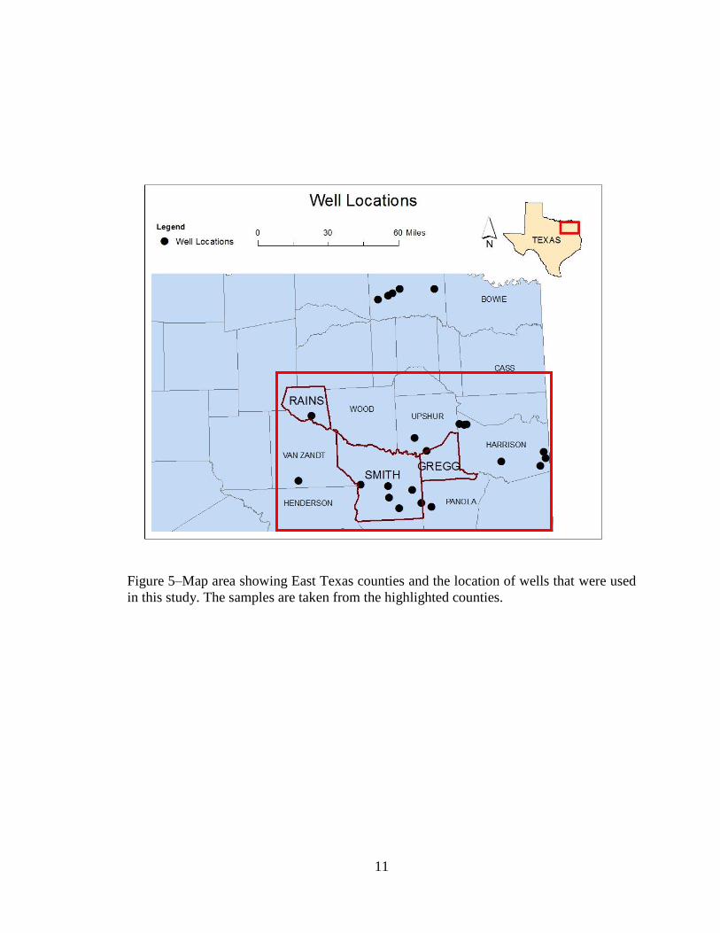
Well sites for potential cores from the East Texas region that must have been used
in this study are shown in Figure 5.

10
Figure 4–Structural cross sections across the East Texas Basin (Wood & Guevara,
1981).
11
Figure 5–Map area showing East Texas counties and the location of wells that were used
in this study. The samples are taken from the highlighted counties.

12
A complex system of rift basins or rhomb grabens were formed on the thinner
continental crust in south Texas, east Texas, north Louisiana, central Mississippi-
southwest Alabama and the Florida Panhandle at the early stage of continental separation
during the Triassic Period. These rift basins and blocks developed into the Rio Grande
embayment, East Texas basin, north Louisiana basin, Mississippi interior basin and the
Apalachicola embayment respectively (Foote, Massingill, & Wells, 1988) (Figure 2). The
Jurassic Louann salt developed in what at the time was a hypersaline restricted basin and
the salt lies unconformably on Triassic rift sediments and Paleozoic basement rock.
Mexia–Talco Fault Zone: Consists of narrow grabens which are formed by strike–
parallel normal faults. “The Great Bend is a zone of en–echelon normal faults which
connect these two zones of parallel faults” (Jackson M. P., 1982). The location of the
Mexia Fault Zone was mainly controlled by Triassic rift faults and by the updip limit of
the Louann Salt, as the fault zone overlies the boundary fault of a half–graben containing
Eagle Mills red beds (Jackson & Harris , 1981).
Central Basin–Faults: This is the salt-pillow province and the salt-diapir province
of the East Texas Basin. Deep subsurface strata are rich in parallel normal faults. These
faults form grabens more than 100 km long, parallel to the Mexia-Talco Fault Zone in
deep Jurassic Strata. Over larger salt-related anticlines, there are faults in the center of the
basin in Cretaceous horizons. On the crests of anticlinal structures such as salt pillows

13
and turtle structures, the orientation of these faults is parallel to the hinge lines of the
anticlines and indicates the splitting of the structures by fold-related extension.
Elkhart Graben: The western end of the Elkhart-Mount Enterprise Fault Zone
consists of the Elkhart Graben. This is made of parallel normal faults which are
approximately 40 km long (Jackson M. P., 1982). “This graben forms the southern
component of a fan of central-basin faults, which trend towards Oakwood Dome on the
southwest margin of the basin (Jackson M. P., 1982)”. The Elkhart Graben’s origin is
derived from the fault geometry which is also applied to the central-basin faults. Collins
and others defined (1980) normal faults which are exposed in the Trinity River along the
strike of the northern flank of the Elkhart Graben.

14
STRATIGRAPHIC SETTING
In the northern Gulf coast, the Cretaceous System is made of 6000 to 9000 feet of
fine to coarse terrigenous and marine clastics, carbonates, and interbedded evaporites and
bioclastic materials (Warner, 1993). Upper Cretaceous units transgressed over older
Mesozoic units because of a significant rise in sea level during the Cretaceous and also
because there was an increase in the subsidence rates in the coastal margins at that time
(Rainwater, Straigraphy and its role in future exploration of oil and gas in Gulf Coast,
1960).
The Cretaceous system can be divided into Upper and Lower Cretaceous series
(Figure 6) (Warner, 1993). The Lower Cretaceous can be further divided into the Hosston
(Travis Peak), Sligo, Pine Island, James, Travis Peak, Ferry Lake, Mooringsport, Paluxy,
Washita – Fredericksburg and Dantzler Formations. The Upper Cretaceous includes the
Tuscaloosa, Eutaw (Austin), and Selma Formations (Dockery, 1981).
A transgression began during the Lower Cretaceous (Hosston) and concluded in a
maximum highstand during the Late Selma which is the closing of the Upper Cretaceous
(Warner, 1993). Sea level reached a maximum highstand during the late Cretaceous and
thereafter the amount of terrigenous materials diminished and subsidence slowed in the
northern Gulf Coast (Warner, 1993).

15
Figure 6–Stratigraphic column of the East Texas basin; highlighted portion showing the
Travis Peak Formation (modified from (Arkansas Geological Survey, 2016)).

16
Figure 7–Structure, top of the Cotton Valley Group Sandstone (base of Travis Peak
Formation), showing the location of this study (modified from (Finley, 1984)).

17
Cotton Valley: The Cotton Valley Group is an Upper Jurassic to Lower
Cretaceous sequence of sandstone, shale, and limestone (Li, 2007). In the study area, the
top of the Cotton Valley ranges from 4,000 ft below sea level in the updip zero region to
more than 13,000 ft below sea level, is the downdip margin.
The Cotton Valley Group and overlying Travis Peak (Hosston) Formation
represent the first major influx of terrigenous clastic sediments into the Gulf of Mexico
Basin (Salvador, 1987). Prodelta, delta-front, and braided-stream facies have been
identified in the Cotton Valley Group in the northwestern part of the East Texas basin
(McGowen & Harris, 1984). The prodelta facies contains minor amounts of very fine-
grained sandstone and siltstone (Li, 2007). Cotton Valley delta-front deposits typically
consist of interbedded sandstone and mudstone with a few thin beds of sandy limestone,
and commonly, they are overlain by a thick wedge of braided-stream sediments
(McGowen & Harris, 1984)
In parts of East Texas, the Travis Peak / Cotton Valley boundary is marked by a
regional transgressive deposit, the Knowles Limestone (Li, 2007). However, the Knowles
Limestone does not extend throughout the East Texas basin (Saucier, 1985), and where it
is absent, Travis Peak sandstones directly overlies Cotton Valley sandstones (Finley,
1984), making correlation of the boundary difficult to impossible.
Bossier Formation: Throughout most of the East Texas, Bossier sequence
is interpreted as marine shale. However, along the south part of the west
flank, well-developed sandstone bodies are interbedded with the marine
shale (Li, 2007). The top of Bossier is approximately 19,000 ft in the deep

18
(Li, 2007). Basinward deterioration of the Bossier reflector may be
attributed to data quality changes in rock properties.
Shuler Formation: They are composed of sandstones, siltstones and shales
deposited in terrigenous, deltaic and nearshore marine environments
(Dickinson, 1969). Deposits unconformably overly the Haynesville
Formation and underlie the Hosston Formation and the Shuler Formation
laterally grades into the Bossier Formation or Cotton Valley Sandstone
(Foote, Massingill, & Wells, 1988).
Travis Peak: The Travis Peak ranges from alluvial fine–grained sands to fine
gravels (Warner, 1993). The sandstones are fine–coarse grained, multicolored, rich in
mica, and are lignitic; the shales and mudstones are multicolored, silty–sandy, rich in
mica, calcareous and are fossiliferous. The Travis Peak Formation overlies the sands and
shales of the Cotton Valley Group (Warner, 1993). Due to the presence of similar rocks,
it is difficult to determine the contact of Lower Cretaceous Travis Peak and the Upper
Jurassic Cotton Valley (Figure 6).
The top of the Travis Peak Formation is transitional and characterized by marine
clastic sediments which grade up toward the Pettet Formation (Li, 2007). Bushaw (1968)
mentioned that during early Travis Peak time, the study area was dominated by alluvial
plane and shoreline environments. However, there was dramtic shift of land during late
Travis Peak–Pettet which resulted in marine sedimentation. “The lower Travis Peak
Formation is composed of thick fluvial channel-fill sandstones deposited by straight
channels, braided streams” (Bushaw, 1968). In the middle and upper Travis Peak

19
Formation, sandstones are braided to meandering, channel-fill deposits that are
interbedded with deltaic deposits (Tye, 1989).
A major sea level regression marks the end of the Cotton Valley age and the
beginning of Travis Peak age (Vail & et al, 1977). The retreating sea plus an increase in
uplift to the north and basin subsidence in the south resulted in extensive erosion in the
coastal plains of the northern Gulf Coast and massive deposition of terrestrial–sourced
clastic sediments in a marginal marine regressive environment (Warner, 1993). The depth
of Travis Peak (Hosston) is shown in Figure (7).
Sligo: The Sligo Formation overlies the Hosston Formation (Figure 6). It is a
gray–brown argillaceous and fossiliferous limestone (Warner, 1993). A period of
continued sea level rise persisted in the Gulf Coast during the early Sligo (Vail & et al,
1977). A regressive sea sequence caused an end to the period of predominant Sligo
carbonate deposition during the end of the Aptian Stage (Warner, 1993).
The Rusk Formation/Glen Rose Formation: Sedimentary patterns within these units
indicate a major withdrawal of the seas which reached a regressive end during the
deposition of the overlying Paluxy Formation (Nichols, 1964). A basal anhydrite member
which was deposited in a mildly regressive environment was the part of basinal facies of
the Rusk Formation (Foote, Massingill, & Wells, 1988) (Figure 6). In the upper part of
the basinal facies are limestones which grade into updip sandstone facies and were
deposited in a minor transgressive cycle. The Rusk/Glen Rose Formation in East Texas is
composed of interbedded shales and limestones which were deposited in shallow marine
environments and some thin strandline sandstones (Foote, Massingill, & Wells, 1988).

20
There is a regional tilt in the area in the northeast Texas which marks the close of the
Trinity group in the Lower Cretaceous period.
Pine Island: This is the oldest formation of the Glen Rose Subgroup, and it is
mostly a carbonate.
James Lime: The James Lime conformably overlies the Pine Island Formation.
The top of the James Lime is picked at the base of the Rodessa (Warner, 1993) (Figure
6).
Rodessa: It conformably overlies the James Lime Formation and is the oldest unit
of Trinity age. It can be difficult to identify in the northern Gulf Coast, because of the
absence of Ferry Lake Anhydrite which separates similar rocks of the Mooringsport
Formation (Warner, 1993). Based on log and sample data it can be identified as a gray,
arenaceous–argillaceous, partly oolitic limestone containing fossil debris and is
interbedded with thin, hard, fine-grained sandstone, brown granular dolomite, gray to
brown red micaceous shale, and white to buff anhydrite stringers (Warner, 1993) (Figure
6).
Ferry Lake: The Ferry Lake Anhydrite is present to the south of the Wiggins Arch,
and when present is a massive, white anhydrite interbedded with thin irregular lenses of
gray shales, limestone and dolomite (Warner, 1993).
Mooringsport: Like the Rodessa Formation, it consists primarily of dark gray–
reddish–brown, oolitic, fossiliferous limestones interbedded with dark gray shale,
multicolored thin sandstone, marl, and thin irregular beds of anhydrite (Warner, 1993).

21
Paluxy: The Paluxy Formation conformably overlies the Mooringsport Formation.
The shales are gray–dark gray, firm–hard, brittle, sandy and calcareous in part whereas,
the sandstone is gray to tan, firm–hard to friable to unconsolidated, poorly sorted,
calcareously cemented, and medium to very fine grained (Warner, 1993).
Washita–Fredericksburg Group: After the deposition of the Paluxy Formation,
there was an advancement of the seas over northeast Texas. As a result, the Goodland
Formation was deposited in a shallow-marine environment during a period of little
sediment influx (Foote, Massingill, & Wells, 1988). Extensive porous facies is exhibited
in the lowermost Goodland Formation which is formed in the extreme northeast corner of
the basin (Eaton, 1956). In the shallow seas the Kiamichi Shale, which consists of fine
grained terrigenous sediments got deposited over the basin (Rainwater, Regional
Stratigraphy and petroleum potential of Gulf Coast Lower Cretaceous, 1970) (Figure 6).
At the time of the deposition of the Washita Group, there were shallow marine seas
which covered the East Texas basin and there prevailed a carbonate depositional
environment over the area of the Angelina-Caldwell flexure (Foote, Massingill, & Wells,
1988). There were limestones deposited on the shelf at the north end of the basin and in
deeper waters to the south, when there was little or no influx of the sediments. The
carbonate formations from oldest–youngest are, the Duck Creek Limestone, Fort Worth
Limestone, Weno-Paw Limestone, Main – Street Limestone, and Buda Limestone (Foote,
Massingill, & Wells, 1988). As shown in Figure 6, there is an interval between the Duck
Creek Limestone and the Main Street Limestone that is equivalent to the Georgetown
Formation.

22
ENGINEERING BEHAVIOR OF SANDSTONES
There have been many studies on sandstones showing the variation in their
geomechanical properties. These variations are mainly due to differences in some
petrographical characteristics which include grain size distribution, packing density,
packing proximity, type of grain contact, length of grain contact, amount of void space,
type and amount of cement/matrix material and mineral composition (Bell, 2007).
Bell & Culshaw (1998) demonstrated that sandstones with smaller mean grain
size possessed higher strength. Sandstones having uniaxial compressive strength in
excess of 40 MPa fall under the category of densely packed (Bell, 2007). UCS is a
compressive strength of the material to withstand loads which has a tendency to reduce
the size. The amount of grain contact was a major influence on the strength and
deformability of sandstones (Dyke and Dobereiner, 1991). The cement content and
interlocking of quartz grains was also considered to be important in terms of strength
and it was also noted that with an increase in cement content there was an increase in the
strength of the rock as the cement helps in binding the grains together (Bell, 2007).
The compressive strength of sandstones is also influenced by the porosity; the
higher the porosity, the lower the strength of the sandstone (Bell, 2007). Moisture content
contained by the sandstones is not an important factor in terms of strength because
Hawkins & McConnell (1992) mentioned that sandstones with significant amount of clay
minerals or rock fragments show loss in wetting, which is due to possible expansion of

23
clay mineral content. The testing of sandstones for indirect tensile strength showed that
the values are almost 1/15th of their compressive strength (Bell, 2007).
Sandstone’s degree of resistance to weathering depends on the mineralogical
composition, amount and type of cement, porosity, type and amount of cement and
lamination (Bell, 2007). Generally, sandstones contain quartz which is highly resistant to
weathering, but the presence of other minerals like feldspar (which maybe kaolinized)
and calcareous cement (which may react in the presence of weak acids) can make
sandstone durability very weak (Bell, 2007). When tested for compressive strength, these
type of sandstones which can be disaggregrated when subjected to saturation have a
compressive strength less than 0.5 MPa (Yates, 1992).

24
UNIAXIAL COMPRESSIVE TEST
Uniaxial compressive strength (σc) is generally known as the boundary between
rocks and soil in rock mechanics and engineering geology, rather than rock texture,
structure or weathering (Palmstrom, 2011). There are many classifications for
compressive strength of rocks, which are presented below in Table 1. The uniaxial
compressive strength of rocks can be determined from direct and indirect tests. Direct
tests include laboratory methods, whereas indirect methods include point load tests. Point
load tests are used to determine rock strength index.
Rock is defined as a naturally occurring material that consists of single or several
minerals which can be held together by a matrix. The highest possible strength limit of a
rock mass can be calculated from uniaxial compressive strength (Palmstrom, 2011).
ISRM (1981) suggests that the uniaxial compressive strength calculated in an area should
be given as the mean strength of the samples as determined away from faults, joints and
other discontinuities to avoid weakness and weathering. When a rock sample is said to be
anisotropic, the value of rock mass index should be tested towards the direction of the
lowest mean strength and in such cases it is highly recommended to measure the uniaxial
compressive strength in all directions (Palmstrom, 2011).
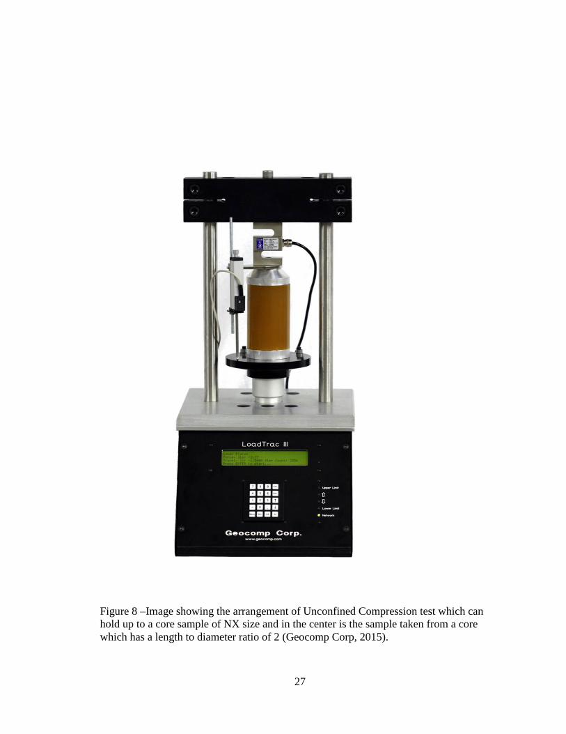
Laboratory testing for uniaxial compressive strength can be time consuming
because it requires precision and accuracy (Figure 9). There are many tests which can be
done in the field to save time, but they may not be accurate as compared to the laboratory

25
tests. The Schmidt hammer test can be used as an alternate to the laboratory test. Strength
can also be assessed non–quantitavely if there is information on the rock like
composition, anisotropy and weathering (Palmstrom, 2011).

26
Tab
le 1
– V
ario
us
stre
ngth
cla
ssif
icat
ion o
f in
tact
rock
(B
ien
iaw
ski,
1984).
27
Figure 8 –Image showing the arrangement of Unconfined Compression test which can
hold up to a core sample of NX size and in the center is the sample taken from a core
which has a length to diameter ratio of 2 (Geocomp Corp, 2015).
28
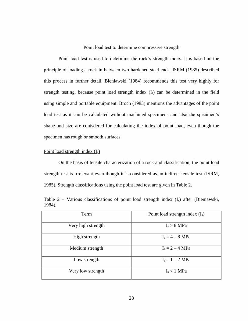
Point load test to determine compressive strength
Point load test is used to determine the rock’s strength index. It is based on the
principle of loading a rock in between two hardened steel ends. ISRM (1985) described
this process in further detail. Bieniawski (1984) recommends this test very highly for
strength testing, because point load strength index (Is) can be determined in the field
using simple and portable equipment. Broch (1983) mentions the advantages of the point
load test as it can be calculated without machined specimens and also the specimen’s
shape and size are conisdered for calculating the index of point load, even though the
specimen has rough or smooth surfaces.
Point load strength index (Is)
On the basis of tensile characterization of a rock and classification, the point load
strength test is irrelevant even though it is considered as an indirect tensile test (ISRM,
1985). Strength classifications using the point load test are given in Table 2.
Table 2 – Various classifications of point load strength index (Is) after (Bieniawski,
1984).
Term Point load strength index (Is)
Very high strength Is > 8 MPa
High strength Is = 4 – 8 MPa
Medium strength Is = 2 – 4 MPa
Low strength Is = 1 – 2 MPa
Very low strength Is < 1 MPa

29
Broch (1983) mentioned that a strength anisotropy index (Ia) can also be measured from
maximum and minimum strength, which are parallel or perpendicular to weakness planes
such as foliation, cleavage, etc (Palmstrom, 2011).
Correlation between point load strength and uniaxial compressive strength
Since the point load test is easy to measure and reliable in some cases it can easily
replace uniaxial compressive tests (Palmstrom, 2011). Hoek & Brown (1980) mentioned
that uniaxial compressive strength is a function of point load strength and is calculated
from the formula:
𝜎𝑐 = 𝑘 × 𝐼𝑠 (1)
Here k is constant value which generally ranges from 15 to 25 and in some cases
between 10 to 50 for anisotropic rocks (Palmstrom, 2011). Research by various authors
has refined this constant as described classification in Table 3.
Table 3 – Various classification of k after (Palmstrom, 2011), where D is diameter.
Authors reference k value
Franklin (1970) k = approx. 16
Broch & Franklin (1972) k = 24
Indian Standards (1998) k = 22
Hoek & Brown (1980) k = 14 + 0.175D
ISRM (1985) k = 20 – 25
Brook (1985) k = 22

30
Ghosh & Srivastava (1991) k = 16
Compressive strength from Schmidt Hammer test
A non–destructive way to approach a compressive test is by performing a Schmidt
Hammer test which measures the rebound hardness of a rock (Palmstrom, 2011). It is
based on the principle that a plunger is released by a spring and it hits the surface of the
rock; the distance of rebound is measured numerically by a scale (Palmstrom, 2011).
Ayday & Goktan (1992) mentioned that the Schmidt Hammer measures rock
properties which are based on elastic impact of two bodies, one of which is impact by the
hammer and the other is impact at the surface of the rock. To measure this impact there
are two types of Schmidt Hammer, they are L and N type Schmidt Hammers shown in
Figure 8 and 9 respectively. These hammers are designed on the basis of impact energy
and the L type Schmidt Hammer has an impact energy of 0.735 N/m, which is 1/3rd of the
N type (Palmstrom, 2011). ISRM (1978) suggested that the L type Schmidt Hammer can
be used for measuring uniaxial compressive strength of rocks which are in the range of
20-150 MPa.

31
A
B
Fig
ure
9 –
L t
ype
Sch
mid
t H
amm
er, w
her
e A
is
the
nee
dle
whic
h i
s p
lace
d a
t th
e su
rfac
e of
the
rock
and B
is
the
scal
e of
the
ham
mer
whic
h i
s u
sed t
o m
easu
re t
he
stre
ngth
in M
Pa
(Pro
ceq
, 2016).
32
Fig
ure
10–N
typ
e S
chm
idt
Ham
mer
, w
her
e A
is
the
nee
dle
whic
h i
s p
lace
d a
t th
e su
rfac
e
of
the
rock
and B
is
scal
e of
the
ham
mer
whic
h i
s u
sed t
o m
easu
re t
he
stre
ngth
in M
Pa
(PC
TE
, 2016)

33
Field Tests To Identify Compressive Strength
The strength of the rocks can be assessed sometimes by using simple field
techniques (Palmstrom, 2011). Based on factors like the hardness of rock, tests for
uniaxial compressive tests can be carried out in the field itself. Table 4 below shows a
general classification of compressive strength based on simple tests done in the field.
These test can be made using a common geological hammer; rock samples should
be at least 10 cm thick and placed on a hard surface. Tests made with one’s hand should
be made on pieces which are 4 cm thick (Palmstrom, 2011). These pieces should not
contain cracks; in different directions of the rock anisotropic tests should be made
(Palmstrom, 2011).
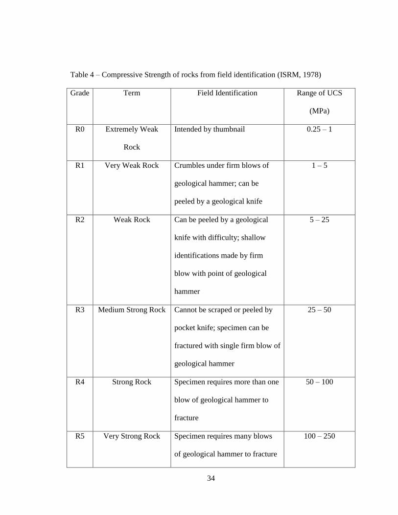
34
Table 4 – Compressive Strength of rocks from field identification (ISRM, 1978)
Grade Term Field Identification Range of UCS
(MPa)
R0 Extremely Weak
Rock
Intended by thumbnail 0.25 – 1
R1 Very Weak Rock Crumbles under firm blows of
geological hammer; can be
peeled by a geological knife
1 – 5
R2 Weak Rock Can be peeled by a geological
knife with difficulty; shallow
identifications made by firm
blow with point of geological
hammer
5 – 25
R3 Medium Strong Rock Cannot be scraped or peeled by
pocket knife; specimen can be
fractured with single firm blow of
geological hammer
25 – 50
R4 Strong Rock Specimen requires more than one
blow of geological hammer to
fracture
50 – 100
R5 Very Strong Rock Specimen requires many blows
of geological hammer to fracture
100 – 250

35
R6 Extremely Strong
Rock
Specimen can only be chipped
with geological hammer
>250

36
TENSILE STRENGTH
Tensile strength is an important property for the strength of a rock because it tells
the vulnerability of the rock towards tensile failure when a load is applied on it (Building
Research Institute, 2016). This test usually results in low strength as compared to the
uniaxial compressive strength test because tensile strength is applied towards the
minimum stress direction, whereas uniaxial compressive strength is applied towards the
maximum stress direction possible. Tensile strength is determined by indirect methods
like 1) Splitting Tensile Test and 2) Flexure Test.
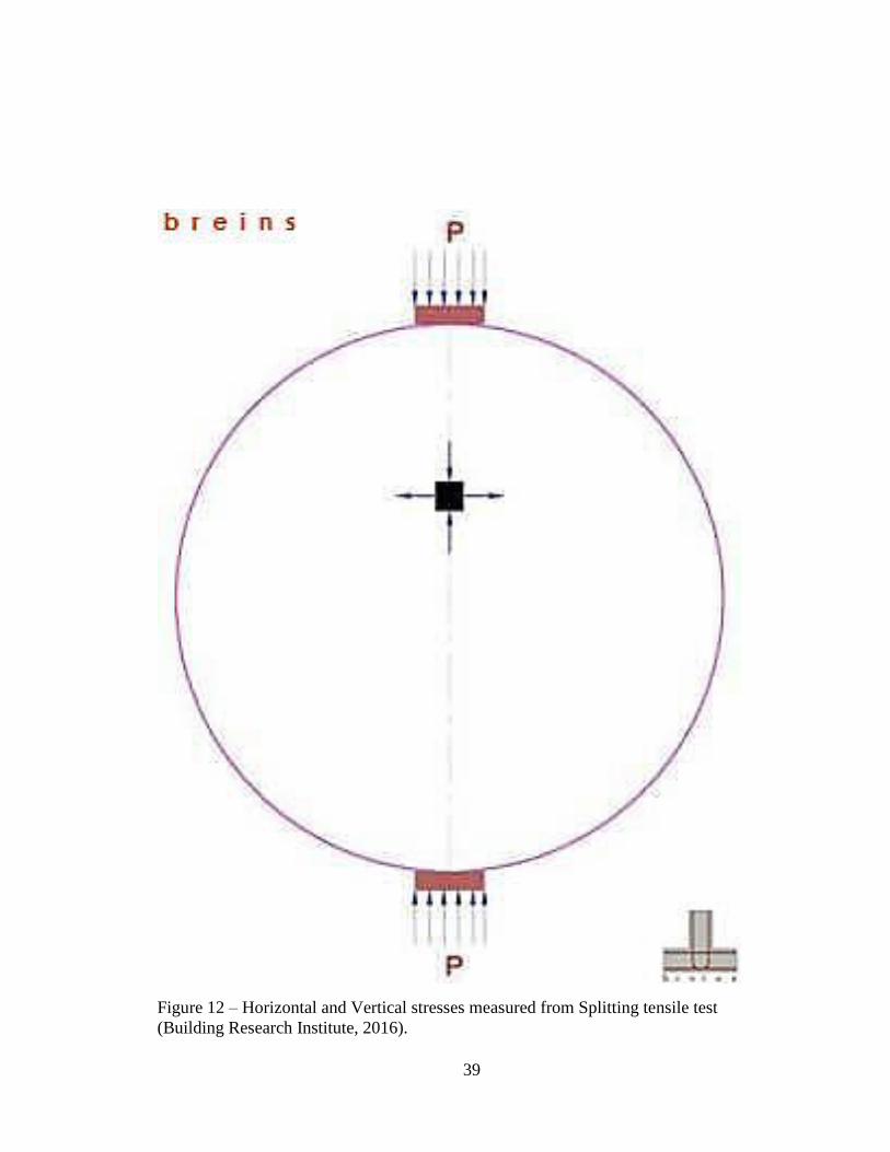
Splitting Tensile Test
ASTM (D 3967-95a) has published a standard procedure for how to test a rock for
splitting tensile strength. The general procedure is to take a sample of NX size, where N
could be any number and X is any unit associated with it. The sample is placed
horizontally in between the loading surface of a compression testing machine (Figure 12).
A load is applied uniformly along the length of the rock sample until it reaches failure.
As the failure is achieved the sample is split into two halves along the vertical
plane because of the indirect tensile stress which is generated due to Poisson’s effect
(Building Research Institute, 2016). “Poisson’s effect is based on the ratio of transverse
contraction strain to longitudinal extension strain in the direction of stretching force”
(Lakes, 2016). Two types of stresses, horizontal and vertical, are developed in this testing
when the compression load is applied (Figure 13). When the loading is applied it is

37
estimated that the compressive stress is acting for about 1/6th of the depth and the
remaining is under tension due to poisson’s effect (Building Research Institute, 2016).

38
Figure 11 – Image showing the arrangement of Tensile strength, which can also hold up a
core size of NX size, and a length to diameter ratio of 4 or 5 (Istone, n.d.)
39
Figure 12 – Horizontal and Vertical stresses measured from Splitting tensile test
(Building Research Institute, 2016).

40
Flexure Test
This is the second most common indirect test done to determine tensile strength.
Generally, it is done for hard rocks or concrete. ASTM D1635 has mentioned general
guidelines to complete the testing. The sample is located at 1/3rd of the distance between
two span points. The standard size of the specimen is 150 x 150 x 750 mm (Building
Research Institute, 2016).
The arrangement is shown in Figure 12. The principle for this test is based on
loads applied equally at a distance of 1/3rd from the bottom of the supporting beam
(Building Research Institute, 2016). Loading is increased with an increase in stress in the
range of 0.02 MPa and 0.10 MPa with the lower rate for low strength rock/concrete and
the higher rate for high strength rock/concrete (Building Research Institute, 2016).
Based on this test, the beam bends at 1/3rd of the area between the applied load
and no shear force is applied in this area, hence it is the area where maximum pure
bending is induced by a shear force of zero (Building Research Institute, 2016).
Maximum tensile stress is reached when a fracture occurs within the middle 1/3rd of the
beam with an increase in load; this is called modulus of rupture fbt, which is calculated
by:
𝒇𝒃𝒕 = 𝑷𝒍 ÷ 𝒃𝒅𝟐 (2)
Where, P = load at failure
l = beam span between supports

41
d = depth of beam
b = width of beam; fbt = modulus of rupture
METHODOLOGY
Sample Preparation and testing
The main aim of this study is to determine the mechanical properties of core
samples from the Travis Peak Formation. Core samples were selected from Stephen F.
Austin State University’s Core Lab Repository and testing for geotechnical properties
was done at the University of Houston. Standard samples were prepared from the selected
cores. The experimental work is mostly based on measuring the load, at the point which
the rock is subjected to stress for both uniaxial compressive strength and tensile strength
tests (Baykasoǧlu, Güllü, Çanakçi, & Özbakir, 2008). All the procedures were based on
guidelines from ASTM D 2938-95 and ASTM D 3967-95a. A total of 12 samples were
subjected to the testing procedure (Table 6).
The UCS test was measured in accordance with ASTM D 2938-95 guidelines.
ASTM is American Society of Testing and Materials, an organization which is associated
for publishing testing standards. ASTM D 2938-95 is a standard publication which deals
with the testing of UCS and also the equipment and preparation of samples. Samples
should have a size ratio of length to diameter of 2:1 for NX size core samples. N is also
referred to any size of the core and X is any unit associated with it. If the sample’s length
to diameter ratio is not 2, then a correction value is applied (ASTM D 2938-95). For
determining tensile strength, the sample size has to be of uniform thickness and width

42
and 2 inches longer than the gauge length (ASTM D 3967-95a). Sample width should not
be less than 5mm, or greater than 25.4mm. Core samples were from the Travis Peak
Formation and were prepared based on the above procedures.
The samples were divided into two sets, one for testing uniaxial compressive
strength (UCS), and the other for testing tensile strength (Figure 14). Samples prepared
for UCS require a base and top to be flattened, which was done by adding Sulfur melted
at 300°F, then let it cool down to solidify and place in the instrument for measuring the
load. Similarly, before working on the tensile strength, all the other parameters that were
used for uniaxial compressive strength were conducted (Figure 15).
Uniaxial compressive strength was tested based on the information from ASTM D
2938-95. Experiments were performed after cutting the edges of the core samples. The
ends were made flat and perpendicular to the axis of the samples so that loads were
applied uniformly (Çanakçi, Baykasoǧlu, & Güllü, 2009). Tensile strength values were
determined indirectly from the Splitting Tensile strength method which was based on
ASTM D 3967-95a. Samples were prepared from the cores. Splitting Tensile strength
was used to test the tensile strength when a cylindrical specimen was subjected to failure,
along the length of specimen under a certain load. The strength classification is given in
the Table 5.

43
Table 5 – Strength classification of intact and jointed rocks (Ramamurthy & Arora,
1993).
Class Description UCS (Mpa)
A Very high strength >250
B High strength 100-250
C Moderate strength 50-100
D Medium strength 25-50
E Low strength 5-25
F Very low strength <5

44
Figure 13–Image showing a core rock sample which was tested for UCS and Tensile
strength which was cut into dimensions of 3.6 in width and 7.2 in length.
7.2
in
3.6 in

45
Figure 14–Equipment used for testing the compressive strength and tensile strength at
University of Houston’s Civil Engineering Laboratory. The same equipment is used to
test the UCS and Tensile strength and the samples are rested on the instrument depending
upon the test and the load is applied.
7.2 in

46
Regression Analysis
Regression analysis can be used to model, examine and predict different
relationships. Why would one use regression analysis? In the view of earth sciences,
regression analysis offers a mathematical relationship between two or more variables
(Maher Jr., 2016). This relationship can be further used to predict one variable from the
known variable.
A linear regression equation is given by the formula 𝑦 = 𝑚𝑥 + 𝑐, where c is the y
intercept and m is the slope of the given line (Figure 20). Linear equations can be positive
or negative, based on the value of slope (Figure 21). The default convention that goes
with regression analysis is that x represents the independent variable and y represents the
dependent variable (Maher Jr., 2016). The predictions of the values of y are made
through the values of x. The dependent variable is sometimes also called a criterion
variable, endogenous variable, prognostic variable, or regressand and the independent
variable is called exogenous variable, predictor variables or regressors (Statistics
Solutions, 2013).
Linear regression involves more than just fitting a line through a set of data
points. This includes a three step process, which is 1) analyze and correlate the data, 2)
estimate the model, which includes the best fit line, and 3) evaluate the usefulness of the
model (Statistics Solutions, 2013).

47
Regression analysis is used for three major purposes. First is the casual analysis,
second is to forecast an effect and third is to forecast a trend (Statistics Solutions, 2013).
Casual analysis is used to identify the strength of the effect that the independent variable
has on a dependent variable. A change in a dependent variable, when subjected to change
in the independent variable, deals with forecasting an effect. Trend forecasting is used to
predict trends and future values.

48
Figure 15–Image showing the equation for the linear regression analysis and the trendline
(University of Washington, 2016).
Figure 16–The above figure shows three different types of linear regression equations.
First image shows a positive trend of the linear equation which has a positive slope.
Second one shows a negative trend of the linear equation which has a negative slope.
Third one is a non-linear equation (Laerd Statistics, 2016).

49
Linear regression can be of two types. First is bivariate regression or simple
regression is associated with one dependent variable and one independent variable.
Second is multivariate or multiple linear regression. It is associated with more than 2
independent variables and one dependent variable. In this study a simple regression or
bivariate regression is used to conduct the statistical analysis.
Independent variables and Dependent variables
Regression equation is the mathematical formula which is applied to the different
variables, so that the dependent variable can be predicted and a model can be estimated
(ESRI, 2016). Unlike in geosciences, where x and y are used as coordinates, here in
regression they are denoted as independent and dependent variables respectively. There is
a regression coefficient associated with the independent variable which describes the
strength and sign of the variable’s relationship to the dependent variable (ESRI, 2016). A
typical regression equation looks like as shown below:
𝒚 = 𝜷𝒙 + 𝜺 (3)
Where,
y = dependent variable
β = coefficient
x = independent variable
ε = Random Error Term

50
Dependent variable (y) – This variable represents the process which is to be
predicted. In the regression equations, they are shown on the left-hand side. To predict
the value using dependent variable, a set of known y values are used to build the
regression model and the known y values are referred as observed values (ESRI, 2016).
Independent variable (x) – This variable is used to predict the variable value of
the model. In a generalized regression equation, they are placed on the right-hand side.
From the equation (3), it can be inferred that dependent variable is a function of
independent variable.
Regression coefficient (β) – This is the value which is estimated from the
regression tools. This value is for independent variable, which represents the strength and
type of relationship between independent and dependent variable (ESRI, 2016). The
coefficient is associated with positive sign, when the relationship is positive and vice-
versa.
P–Values – Regression methods perform statistical tests to measure the
significance of a coefficient by using a p-value. Null hypothesis for statistical tests shows
that a coefficient is not significantly different zero (ESRI, 2016). Small p-values reflect
small probabilities, which suggest that coefficient is important to the model, whereas
coefficient estimates with near zero values do not help in predicting the model and are
removed from the regression equations (ESRI, 2016).
R2/R-squared – R-squared and adjusted R-squared values are both derived from
the regression equation to check the performance of the model. The value of R-squared

51
ranges from 0 to 100 percent, R-squared is 1.0 when the model fits perfectly and there is
no error (ESRI, 2016). However, this happens in the case when a prediction is made of a
form of y to predict y. A scatterplot showing the estimated and predicted values can be
very useful in understanding the R-squared values. Adjusted R-squared is always less
than R-squared because it reflects the complex number of variables (ESRI, 2016).
Residuals – They are the unexplained portion of the dependent variable, shown in
the regression equation as ε. Using values which are known for dependent variables and
independent variables, regression equation will predict y values (ESRI, 2016). Residuals
are also known as the difference between the observed y values and predicted y values.
Large values of residuals indicate a poor fit.
Regression model is a process which deals with an iterative process, which
involves finding an effective independent variable to explain the model and then
removing the variables which are not good for the model (ESRI, 2016).

52
RESULTS
Uniaxial Compressive Strength
Core rock samples from the Travis Peak Formation in East Texas were used in
this study. A map showing the location of the samples is shown in Figure 5. Cores
selected for testing were half core rock samples. An extensive investigation was carried
out to select the sandstone blocks of core samples from the Travis Peak Formation.
Samples were selected carefully from the Stephen F. Austin State University’s Core Lab
Repository (Figure 14).
During the experimental work, the load for uniaxial compressive strength was
calculated from the compressive strength instrument at University of Houston’s
Department of Civil Engineering Laboratory (Figure 15). Overall 12 samples were tested
for uniaxial compressive strength. All the tests were followed under the specifications of
(ASTM D 2938-95).
The samples were cut by a saw. All the samples were from NX size, where N was
4 inches. The height to diameter ratio was 2. In order to make the samples flat, they were
layered with Sulfur melted at 300° F (Figure 22). As per norms of (ASTM D 2938-95)
the sample was placed vertically under the instrument and tested until it reached failure
by breaking; this is the point where the stress is maximum σ1 (Figure 23). The load was
calculated in poundsforce (lbf).
Uniaxial compressive strength was calculated from the formula:

53
𝑼𝑪𝑺 (𝒍𝒃𝒇
𝒊𝒏𝟐⁄ ) = 𝑳𝒐𝒂𝒅 (𝑷 𝒊𝒏 𝒍𝒃𝒇)
𝑨𝒓𝒆𝒂 (𝒊𝒏𝒄𝒉𝒆𝒔𝟐) (4)
Then uniaxial compressive strength was converted to SI Units by 1 lbf/in2 = 6.894
KPa.
All the calculated UCS are shown in the Table 7.

54
Figure 17–Top and bottom of the samples are flattened by adding Sulfur which is melted
at 300° F. Cores are made flat so that they are stable when subjected to stress.

55
Figure 18–Failure from the maximum stress plane (σ1) results in the uniaxial
compressive strength test. In this figure the three different stress planes are shown which
are associated with uniaxial compressive strength. This image is captured after the UCS
has been achieved.
σ1
σ1
σ3 σ3
σ2
σ2
56
The uniaxial compressive strength test of the samples has a range between 13.23
and 45.87 MPa with an average value of 27.43 MPa and standard deviation of 9.47. A
frequency distribution histogram is plotted for the uniaxial compression strength, which
shows major population in the range of 28.23 and 43.23 MPa (Figure 24). It also shows a
nearly normal distribution of the samples. Based on the frequency and mean the rocks
can be classified as medium strength (Table 5).

57
Tensile Strength
Core rock samples of the Travis Peak Formation in East Texas were collected
from Stephen F. Austin State University core lab repository (Figure 15). An experiment
of splitting tensile strength was completed at University of Houston’s Department of
Civil Engineering Laboratory (Figure 14). These cores were measured for splitting tensile
strength using the same instrument which measured compressive strength.
Twelve samples were tested for splitting tensile strength. All the tests were
followed under specifications from (ASTM D 3967-95a). The samples were prepared
first by cutting with a saw. Samples of NX size were used, where N is 4 inches and the
height to diameter ratio was 2.
The samples were placed horizontally under the instrument compression was
applied and testing was stopped when the rock broke from the area where minimum
stress was applied, σ3 (Figure 25). The load was measured from the instrument in
pounds*force (lbf).
Splitting tensile strength was calculated from the formula:
𝑻 = 𝟐𝑷
𝝅𝑫𝑳 (5)

58
Figure 19–A plot showing the frequency histogram for UCS with the maximum number
of 6 samples lie in the range of 28.23 to 43.23 MPa and minimum number of 1 sample
lying in the range of 43.23 to 58.23 MPa.

59
Figure 20–Failure from minimum stress plane (σ3) results in tensile strength. Three
different stress axes associated with the tensile strength are shown in this figure. Figure is
captured after tensile strength has been achieved.
σ1 σ1
σ3
σ3
σ2
σ2

60
Where T is tensile strength in lbf/in2, P is load applied in lbf, D is diameter of the sample
in inches and L is the length of the sample in inches.
Splitting tensile strength was converted to SI units (MPa) by 1 lbf/in2 = 6.894
KPa. The calculated tensile strength is shown in the Table 7.
The tensile strength of the samples had a range between 1.69 MPa and 6.32 MPa
with an average value of 3.97 MPa and standard deviation of 1.25. A frequency
distribution histogram was plotted, which shows major population in the range of 3.59
and 5.49 (Figure 26). This also shows a near normal distribution of the samples. Hsu &
Nelson stated that tensile strength is not valid for soft rock based on the theory of brittle
failure, but compressive strength shows that the rock is of medium strength.

61
Figure 21–A plot showing the frequency histogram for Tensile strength, where the
maximum number of 6 samples lying in the range of 3.59 to 5.49 MPa and a minimum of
2 samples lying in the range of 5.49 to 7.39 MPa.

62
Regression Analysis
Uniaxial Compressive Strength vs Tensile Strength
A simple regression analysis was calculated to relate uniaxial compressive
strength and tensile strength. The data which are shown in Table 6 are used in the
regression analysis approach. The input variable is the load for uniaxial compressive
strength (X1) and the output variable is tensile strength (Y1). The equations which are
obtained from the analysis were used in predicting the UCS values. Matlab software was
used to carry out the simple linear regression analysis.
Regression equations obtained from the analysis are shown below:
𝒀𝟏 = 𝟎. 𝟏𝟎𝟎𝟓 ×𝑿𝟏 + (𝟏. 𝟐𝟗𝟑) (6)
R – square of the predicted uniaxial compressive strength from the regression
analysis is 0.6378. The test results of the simple regression analysis are shown in Figure
(22).

63
Fig
ure
22–A
plo
t sh
ow
ing l
inea
r re
gre
ssio
n a
nal
ysi
s bet
wee
n U
nia
xia
l
Com
pre
ssiv
e S
tren
gth
an
d T
ensi
le s
tren
gth
whic
h h
as a
R-s
quar
e val
ue
of
0.6
378.

64
Box Plots
Box plots are one of the tools which are used for depicting location and changes
in information among data sets, particularly to see changes in variation among different
groups of data (Chambers, Cleveland, Kleiner, & Tukey, 1983). The vertical axis in a box
plot represents the response variable and the horizontal axis is the factor of interest. A
box plot is completed by calculating the median and quartiles; the lower quartile is the
25th percentile and the upper quartile is the 75th quartile (NIST, 2016). A box plot is
drawn when a symbol is placed at the median which is in between the lower and upper
quartiles; this is the main body of the data and a line is drawn from the lower quartile to
the minimum point and another from the upper quartile to the maximum point (NIST,
2016).
There are four major points in a box plot. The first point is the minimum point;
the second point is the difference between the lower quartile and the minimum point; the
third point is the difference between the upper quartile and the lower quartile and the
fourth point is the difference between the maximum point and the upper quartile. The
reason for using a box plot is to determine if a factor has a significant effect on the
response with respect to either location or variation (NIST, 2016).
Box plots showing the variation in UCS and Tensile strength are shown in Figure
(28).
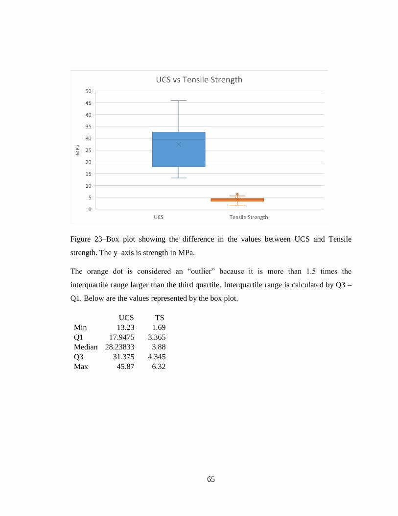
65
Figure 23–Box plot showing the difference in the values between UCS and Tensile
strength. The y–axis is strength in MPa.
The orange dot is considered an “outlier” because it is more than 1.5 times the
interquartile range larger than the third quartile. Interquartile range is calculated by Q3 –
Q1. Below are the values represented by the box plot.
UCS TS
Min 13.23 1.69
Q1 17.9475 3.365
Median 28.23833 3.88
Q3 31.375 4.345
Max 45.87 6.32

66
Table 6–Table showing the data generated from the laboratory equipment for UCS and
Tensile strength.
Samples UCS Load
(lbf)
Tensile
Load (lbf)
Area
(square
inches)
UCS
(lbf/in2)
Tensile
Strength
(lbf/in2)
UCS
(Mpa)
Tensile
Strength
(Mpa)
1 27580.42 13194.05 7.94 3473.6 1057.88 23.95 4.01
2 38623.84 15049.72 7.13 5417.09 1343.75 37.35 4.83
3 38511.99 15295.28 8.8 4376.36 1106.51 30.17 4.42
4 32720.08 10602.34 7.94 4120.92 850.01 31.63 3.4
5 47435.12 20798.41 7.13 6652.89 1857.04 45.87 6.32
6 37741.43 14603.07 8.36 4514.53 1112.03 31.12 4.32
7 33458.2 12849.63 8.8 3802.07 929.58 18.38 3.71
8 26473.15 10713.04 7.94 3334.15 858.96 29.05 3.26
9 16927.49 8345.24 7.13 2374.12 745.13 16.37 2.68
10 14448.76 5405.68 7.53 1918.83 457.02 13.23 1.69
11 20189.32 10780.51 8.36 2414.99 820.94 16.65 4.37
12 40713.56 18398.33 7.94 5127.65 1475.16 35.35 5.59

67
DISCUSSION
Core rock samples of the Travis Peak Formation were collected from Stephen F.
Austin State University’s core lab repository. Overall 12 samples were collected from
different counties based on the depth interval of more than 7500 ft. Samples were
restricted to sandstones and any core rocks containing carbonates were avoided.
Sandstone samples and carbonate samples like dolomite, limestone, etc., were
differentiated by using hydrochloric acid (HCl). If HCl gave a fizz when dropped over
the rock samples then it was said to be a carbonate rock; when it did not give any fizz the
sample was shown to be a sandstone.
The selected core samples were then cut into a size of 7.2 to 3.6 (in) ratio of
length to diameter maintaining the 2 to 1 ratio. Samples were then tested for uniaxial
compression test and tensile strength in the Department of Civil Engineering Laboratory
at University of Houston. After these tests were performed a regression analysis was used
to test the accuracy of the results.

68
CONCLUSIONS
In this study a statistical method, regression analysis was carried out to formulate
a model that may be used to predict the values of tensile strength given the UCS.
Laboratory tests were performed to measure the uniaxial compressive strength and tensile
strength of core rock samples of the Travis Peak Formation from certain counties in East
Texas.
Uniaxial compressive strength was calculated from the load, which was measured
using a compressive test instrument. Load is generated when there is failure at the
maximum stress plane (σ1). The maximum UCS observed using laboratory tests was
45.87 MPa and the minimum was 13.23 MPa. The average value of UCS for the 12
samples was 27.43 MPa and the standard deviation was 9.47.
Similarly, tensile strength was calculated from the load which was also measured
from the same compressive testing instrument. Here, the failure was achieved at the
minimum stress plane (σ3). The maximum tensile strength observed during the laboratory
tests was 6.32 MPa and the minimum was 1.39 MPa. The average value of tensile
strength for 12 samples tested was 4.05 MPa and the standard deviation was 1.25.
From Table 5, the rock samples belong to class D, which are medium strength
rocks. This can be justified by the mean of the UCS for the rock samples which was 27.
43 MPa; Class D classification has a UCS of range 25 – 50 MPa.

69
Linear regression analysis was performed to build a model so that the values for
tensile strength may be predicted given the USC. The R-squared value for the regression
analysis was 0.6378, which indicates the model fits fairly well. The slope of the
regression equation is 0.1005 which indicates that for each uniaxial compressive strength
value the tensile strength is increased by an estimated value of 0.1005.

70
FUTURE WORK
This study measured the geotechnical properties of core rocks from the Travis
Peak Formation. More geotechnical properties could be measured, like the different types
of UCS which includes UCS from Schmidt Hammer and Point load tests depending upon
the availability and accessibility to the instruments.
More samples could be collected depending upon the availability and all the
necessary factors which were used in this study. More accurate results could be acquired
if a larger dataset was used. Some tests that could be done while performing UCS would
be specific gravity test, water saturation and dry density.
Soft computing techniques like genetic programming and grey systems will be
very useful in comparing the prediction of UCS and tensile strength. Also, different
carbonate rocks found in the Travis Peak Formation can also be tested. Then a
comparison can be made between the strength of different rock types.
71
REFERENCES
Arkansas Geological Survey. (2016, June 6). Oil: Petroleum Geology of Producing Area.
Retrieved from http://www.geology.ar.gov/energy/oil_prodarea.htm
Arora, M. K., Das Gupta, A. S., & Gupta, R. P. (2004). An artificial neural network
approach for landslide hazard zonation in the Bhagirathi (Ganga) Valley,
Himalayas. International Journal of Remote Sensing, 559-572.
ASTM D 2938-95. (n.d.). Standard Test Method for Unconfined Compressive Strength of
Intact Rock Core Specimens.
ASTM D 3967-95a. (n.d.). Standard Testing Method for Splitting Tensile Strength of
Intact Rock Core Specimens.
ASTM D1635. (n.d.). Standard Test Method for Flexural Strength of Soil-Cement Using
Simple Beam with Third-Point Loading.
Ayday, C., & Goktan, R. M. (1992). Correlations between L and N type schmidt hammer
rebound values obtained during field testing. Eurock, (pp. 47-49).
Baykasoǧlu, A., Güllü, H., Çanakçi, H., & Özbakir, L. (2008). Prediction of compressive
and tensile strength of limestone via genetic programming. Expert Systems with
Applications, 111-123.
Bell, F. G. (2007). Engineering behaviour of sedimentary rocks. In F. G. Bell,
Engineering Geology (pp. 259-262). Butterworth-Heinemann.
Bell, F. G., & Culshaw, M. G. (1998). Petrographic and engineering properties of
sandstone from the Sneinton Formation, Nottinghamshire, England . Quaterly
Journal Engineering Geology, 5-21.
Bieniawski, Z. T. (1984). Rock mechanics design in mining and tunnelling. In Z. T.
Bieniawski, Rock mechanics design in mining and tunnelling (p. 272). Balkema,
Rotterdam.
Boersma, P., & Weenink, D. (2004, May 11). Feedforward neural networks 1. What is a
feedforward neural network? Retrieved from Praat: doing phonetics by computer:
http://www.fon.hum.uva.nl/praat/manual/Feedforward_neural_networks_1__Wha
t_is_a_feedforward_ne.html
Broch , E., & Franklin, J. A. (1972). The point load strength test. International Journal of
Rock Mechanics and Mining Sciences, 669-697.
72
Broch, E. (1983). Estimation of Strength Anisotropy Using the Point Load Test.
International Journal of Rock Mechanics and Mining Sciences, 181-187.
Brook, N. (1985). The equivalent core diameter method of size and shape correction in
point load testing. International Journal of Rock Mechanics Mining Sciences and
Geomechanics, 61-70.
Building Research Institute. (2016, June 1). Material Testing. Retrieved from Tensile
Test on Concrete: http://www.buildingresearch.com.np/services/mt/mt2.php
Bushaw, D. J. (1968). Environmental synthesis of the East Texas Lower Cretaceous:
Transactions. Gulf Coast Association of Geologial Societies, v. XVIII, 416-438.
Çanakçi, H., Baykasoǧlu, A., & Güllü, H. (2009). Prediction of compressive and tensile
strength of Gaziantep basalts via neural networks and gene expression
programming. Neural Computing and Applications, 1031-1041.
Chambers, J., Cleveland, W., Kleiner, B., & Tukey, P. (1983). Graphical Methods for
Data Analysis. Wadsworth.
Collins , E. W., Hobday, D. K., & Kreitler, C. W. (1980). Quaternary faulting in East
Texas. Austin: University of Texas at Austin, Bureau of Economic Geology
Geologic Cicrular.
Congalton, R. G. (1991). A review of assessing the accuracy of classifications of
remotely sensed data. Remote Sensing Environment, 35-46.
Davidoff, A. J. (1991). Evidence for a deep Mesozoic basin in central east Texas;
implications for hydrocarbon exploration. Gulf Coast Association of Geological
Societies, 143-151.
Dickinson, K. A. (1969). Upper Jurassic carbonate rocks in northeastern Texas and
adjoining parts of Arkansas and Louisiana . Gulf Coast Association of Geological
SocietiesTransactions, 175-187.
Dockery, D. T. (1981). Stratigraphic coumn of Mississippi . Mississippi Bureau of
Geology.
Eaton, R. W. (1956). Resume of subsurface geology of northeast Texas with emphasis on
salt structures. Gulf Coast Association of Geological Societies Transactions, 79-
84.

73
ESRI. (2016, May 23). Regression Analysis Basics. Retrieved from Regression Analysis
Basics:
http://resources.esri.com/help/9.3/arcgisdesktop/com/gp_toolref/spatial_statistics_
toolbox/regression_analysis_basics.htm
Fener, M., Kahraman, S., Bilgil, A., & Gunaydin, O. (2005). A comparitive evaluation of
indirect methods to estimate the compressive strength of rocks. Rock Mech Rock
Eng, 329-343.
Finley, R. J. (1984). Geology and engineering characteristics of selected low-
permeability gas sandstones: a national survey:. Austin: The University of Texas
at Austin, Bureau of Economic Geology, Report of Investigations.
Foote, R. Q., Massingill, L. M., & Wells, R. H. (1988). Petroleum geology and the
distribution of conventional crude oil, natural gas, and natural gas liquids, East
Texas basin. U.S. Geological Survey Open-File Report.
Franklin, J. A., & Hoek, E. (1970). Developments in triaxial testing technique. Rock
Mechanics, 223-280.
Galloway, W. E. (2009). The Gulf of Mexico Basin has proved to be a highly successful
hydrocarbon province, and the vast untapped volume of both oil and gas ensures
that the basin will continue as a major player for decades to come. GeoExPro.
Garret, J. H. (1994). Where and why artifical neural networks are applicable in civil
engineering. Journal of Computing in Civil Engineering, 129-130.
Geocomp Corp. (2015). Geocomp Corporation. Retrieved from Geocomp:
http://www.geocomp.com/images/prod_images/Unconfined-Compression-
mini.jpg
Gershenson, C. (2003). Artifical Neural Network for beginners. Cornell University.
Ghosh, D. K., & Srivastava, M. (1991). Point load strength: An index for classification of
rock material. Bulletin of International Association of Engineering Geology, 27-
33.
Hawkins, A. B., & McConnell, B. J. (1992). Sensitivity of sandstone strength and
deformability to changes in moisture content. Quaterly Journal Geological
Society, 115-129.
Hoek, E., & Brown, E. T. (1980). Empirical strength criterion for rock masses. Journal of
Geotechnical Engineering, ASCE, 1013-1035.

74
Hsu, S. C., & Nelson, P. P. (2002). Characterization of Eagle Ford Shale. Engineering
Geology, 151-5.
Indian Standards. (1998). Method for determination of point load strength index of rocks.
New Delhi: Bureau of Indian Standards.
ISRM. (1978). Standardization of laboratory and field tests. International Journal of
Rock Mechanics Mining Sciences and Geomechanics, 319-368.
ISRM. (1981). Rock characterization testing and monitoring. Oxford: Pergamon Press.
ISRM. (1985). International Society of Rock Mechanics Commisssion on Testing
Methods, Suggested Method for Determining Point Load Strength. International
Journal of Rock Mechanics and Mining Sciences, 51-60.
Istone. (n.d.). Tensile Strength. Retrieved from Istone:
http://www.istone.ntua.gr/Training_courses/wp1/3-2-4c-2.jpg
Jackson, M. P. (1982). Fault tectonics of the East Texas Basin. Bureau of Economic
Geology, Geological Circular, 31.
Jackson, M. P., & Harris , D. W. (1981). Sesimic Stratigraphy and salt mobilization
along the northwestern margin of the East Texas Basin, in Kreitler, C. W., and
others, Geology and geohydrology of the East Texas Basin: a report in the
progress of nuclear waste isolation feasibility studies. Austin: The University of
Texas at Austin, Bureau of Economic Geology Geological Circular 81-7.
Jackson, M. P., & Seni, S. J. (1984). Atlas of salt domes in the East Texas basin. Bureau
of Economic Geology, The University of Texas at Austin.
Jacobson, L. (2013, December 5). Introduction to Artificial Neural Networks. Retrieved
from The Project Spot: http://www.theprojectspot.com/images/post-assets/an.jpg
Laerd Statistics. (2016, May 23). Linear Regression Analysis using SPSS Statistics.
Retrieved from Laerd Statistics: https://statistics.laerd.com/spss-tutorials/linear-
regression-using-spss-statistics.php
Lakes, R. (2016, October 9). What is Poisson's Ratio? Retrieved from Meaning of
Poisson's ratio: http://silver.neep.wisc.edu/~lakes/PoissonIntro.html
Levenberg, K. (1944). A Method for the Solution of Certain Non-linear Problems in
Least Squares. Quaterly of Applied Mathematics, 164-168.

75
Li, Y. (2007, May). Evaluation of Travis Peak Reservoirs, west margin of the East Texas
Basin. College Station, Texas, USA.
Maher Jr., H. D. (2016, May 23). Geoscience Data Analsysis and Modeling. Retrieved
from University of Nebrakska Omaha:
http://maps.unomaha.edu/maher/GEOL2300/week3/week3.html#anchor438704
Marquardt, D. W. (1963). An Algorithm for the Least-Squares Estimation of Nonlinear
Parameters. SIAM Journal of Applied Mathematics, 431-441.
Martin, R. G. (1978). Northern and eastern Gulf of Mexico continental margin
stratigraphic and structural framework, in Bouma, A. H., Moore, G. T., and
Coleman, J. M., eds., Framework, facies, and oil-trapping charactersitics of the
upper continental margin. American Association of Petroleum Geologists Studies
in Geology, 21-42.
Martin, R. G. (1984). The regional geology, petroleum potential environmental
considerations for development, and estimates of undiscovered recoverable oil
and gas resources of the United States Gulf of Mexico Continental Margin in the
area of proposed Oil and Gas Lease Sales. U.S. Geological Survey Open-File
Report.
Matlab. (2005). Neural Network Toolbox. Retrieved from Conjugate Gradient Algorithms
: Backpropagation: http://matlab.izmiran.ru/help/toolbox/nnet/backpr59.html
Mazur, M. (2015, March 17). A step by step back propogation example. Retrieved from
https://mattmazur.com/2015/03/17/a-step-by-step-backpropagation-example/
McGowen, M. K., & Harris, D. W. (1984). Cotton Valley (Upper Jurassic) and Hosston
(Lower Cretaceous) depositional systems and their influence on salt tectonics in
the East Texas Basin: in W. P. S. Ventress et al., eds., The Jurassic of the Gulf
Rim; Gulf Coast Section SEPM Foundation,. Third Annual Research Conference
Proceedings, (pp. 213-253).
Meulenkamp, F. (1997). Improving the prediction of the UCS, by equotip readings using
statistical and neural network models. Mem Cent Eng Geol Neth, 162:127.
Murray , G. E., & Others. (1985). Introduction to the habitat of petroleum, northern Gulf
(of Mexico) coastal province, in Perkins, B. F., and Martin, G. B., Habitat of oil
and gas in the Gulf Coast. Society of Exonomic Paleontologists and Mineralogists
Foundation, (pp. 1-24).
Newkirk, T. F. (1971). Possible future petroleum potential of Jurassic, western Gulf
basin, in Cram, I. H. (ed.), Future petroleum provinces of the United States - their
76
geology and potential. American Association of Petroleum Geologists memoir,
927-953.
Nichols, P. H. (1964). The remaining frontiers for exploration in northeast Texas. Gulf
Coast Association of Geological Societies Transactions, 7-22.
NIST. (2016). Engineering Statistics Handbook. Retrieved from Box Plot:
http://www.itl.nist.gov/div898/handbook/eda/section3/boxplot.htm
Palmstrom, A. (2011, March 12). Rmi - A rock mass characterization system for rock
engineering purposes. PhD Thesis. Oslo, Norway: Oslo University.
PCTE. (2016, May 31). PCTE. Retrieved from The Original Schmidt Hammer:
http://pcte.com.au/images/NDT-Equipment-images/SchmidtHammer/2.jpg
Presco. (2013). Presco Inc.,. Retrieved from
http://www.prescocorp.com/projects/east%20texas/stratcolumn.gif
Proceq. (2016, May 31). Proceq. Retrieved from Proceq USA E Shop: http://shop-
usa.proceq.com/product_info.php?cPath=0_23_91_97&products_id=167&osCsid
=i9jqk0bcv3g2m4ugotdb2to7g5
Rainwater, E. H. (1960). Straigraphy and its role in future exploration of oil and gas in
Gulf Coast. Gulf Coast Association of Geological Societies Transactions, 33-75.
Rainwater, E. H. (1968). Geological history of oil and gas potential of the Central Gulf
Coast. Gulf Coast Association of Geological Societies Transactions, 124-165.
Rainwater, E. H. (1970). Regional Stratigraphy and petroleum potential of Gulf Coast
Lower Cretaceous. Gulf Coast Associaition of Geological Societies Transactions,
145-157.
Ramamurthy, T., & Arora, V. K. (1993). A classification for intact and jointed rocks.
Geotechnical engineering of hard soils-soft rocks, 235-242.
Rao, K. S., Rao, G. V., & Ramamurthy, T. (1987). Strength of sandstones in saturated
and partially saturated conditions. Geotechnical Engineering, 99-127.
Salvador, A. (1987). Late Triassic-Jurassic paleogeography and origin of Gulf of Mexico
Basin. AAPG Bulletin, 419-451.
Saucier, A. E. (1985). Geologic Framework of Travis Peak (Hosston) Formation of East
Texas and Louisiana, in Finley, R. J., et al., The Travis peak Formation: Geologic
Framework, core studies and engineering field analysis. The University of Texas
at Austin, Bureau of Economic Geology, contract report n0. GRI-85/0044
prepared for the Gas Research Institute under contract no. 5082-211-0708.

77
Schalkoff, R. J. (1997). Artificial Neural Networks. McGraw-Hill.
Seibi, A., & Al-Alawi, S. M. (1997). Prediction of fracture toughness using artificial
neural networks. Engineering Fracture Mechanics, 311-319.
Singh, V. K., Singh, D., & Singh, T. N. (2001). Prediction of strength properties of some
schistose rocks from petrographic properties using artificial neural networks.
International Journal of Rock Mechanics and Mining Sciences , 269-284.
Statistics Solutions. (2013). What is Linear Regression. Retrieved from Statistics
Solutions: http://www.statisticssolutions.com/what-is-linear-regression/
Tye, R. S. (1989). Fluvial sandstone reservoirs of Travis Peak (Hosston) Formation, East
Texas Basin. AAPG Bulletin, v. 73, 421.
University of Washington. (2016, May 23). Linear Regression. Retrieved from ATM S
451 Lab Manual:
http://www.atmos.washington.edu/~robwood/teaching/451/labs/linearregression.h
tml
Vail, P. R., & et al. (1977). Seismic stratigraphy and global changes of sea level. Seismic
stratigraphy - applications to hydrocarbon exploration (pp. 49-212). American
Association of Petroleum Geologists.
Warner, J. A. (1993). Regional geologic framework of the Cretaceous, offshore
Mississippi. Jackson: Mississippi Department of Environmental Quality.
Wood, D. H., & Guevara, E. H. (1981). Regional structural cross sections and general
stratigraphy, East Texas Basin. Austin: The University of Texas at Austin,
Bureau of Economic Geology Cross Sections.
Yates, P. G. (1992). The material strength of sandstones of the Sherwood Sandstone
Group of north Staffordshire with reference to microfabirc. Quaterly Journal
Geological Society, 107-113.

78
APPENDIX A – CORE SAMPLES DATABASE
Table 7 - Table showing details on the core samples that must be used for the testing.
API NumberOfBoxes X Y Depth County
03730288 17 -94.0674141 33.3180697 9000 Bowie
06730432 2 6100 Bowie
06730434 2 -94.1361712 32.9964246 6100 Bowie
06730469 2 -94.1328450 33.0016427 6100 Bowie
06730472 1 -94.1428303 32.9881211 6093 Bowie
06730475 2 -94.1203544 33.0064686 6100 Bowie
06730477 2 -94.1237491 33.0065534 6100 Bowie
06730478 2 -94.1183602 33.0093725 6100 Bowie
06730482 2
06730484 2 -94.1217662 33.0089595 6100 Bowie
06730488 2 -94.1143441 33.0099487 6100 Bowie
06730489 2 -94.1412647 32.9854973 6100 Bowie
06730547 20 -94.1140637 33.0077657 6100 Bowie
06730577 2 -94.1381949 32.9770992 6100 Bowie
06730714 18 -94.0674045 33.0241065 6100 Bowie
10539584 126 -101.9040465 30.9620919 6100 Bowie
10539639 131 -101.8844747 30.9692479 6100 Bowie
10539658 4 -101.8992749 30.9725194 6100 Bowie
10539819 2 -101.8683593 30.9835001 6100 Bowie
10539885 2 -101.8520433 30.8987167 6100 Bowie
10539889 65 -101.8781112 30.9805555 6100 Bowie
10539910 50 -101.8030972 30.9415267 6100 Bowie
10540041 2 -101.8986619 30.9945668 6100 Bowie
10540055 27 -101.8454651 30.919604 6100 Bowie
10540290 101 -101.830308 30.886847 6100 Bowie
10540334 18 -101.833909 30.887273 6100 Bowie
10540345 1 -101.8383039 30.882586 6100 Bowie
16131229 25 -96.3418012 31.7362474 12000 Freestone
16131409 5 -96.2223344 31.6203672 12000 Freestone
18330958 8 -94.8319258 32.5383259 7500 Freestone
18331297 21 -94.9334652 32.5505917 10000 Gregg

79
20332171 3 -94.0785006 32.5097246 5900 Gregg
20332249 15 -94.1103075 32.4230525 2700 Gregg
20332253 5 -94.0679832 32.469908 2700 Gregg
20332348 9 -94.649061 32.7018649 3700 Gregg
20332350 1 -94.6870034 32.7093313 3800 Gregg
20332415 20 -94.6337798 32.7034887 3600 Gregg
20332558 5 -94.392921 32.4646912 6000 Gregg
21330756 35 -95.571681 32.0686618 9900 Gregg
21330787 6 -95.93317 32.0932446 8400 Henderson
26932697 1 -100.0611654 33.6986735 8400 Henderson
27730116 6 -95.4043176 33.5384112 8400 Henderson
31530855 4 -94.2468561 32.7741368 8400 Henderson
31530874 2 -94.2498675 32.7770898 8400 Henderson
36501107 4 -94.1186202 32.1811946 3080 Henderson
36530251 13 -94.2259916 32.0975177 2050 Henderson
36533070 52 -94.0855906 32.3779916 4900;6000 Henderson
36533106 14 -94.0849156 32.3814072 6000 Henderson
36534070 20 -94.2701039 32.2419251 2000 Henderson
36534131 7 -94.2580663 32.2433188 1900 Henderson
36534339 17 -94.2329432 32.1307754 2400 Henderson
36534412 14 -94.2086483 32.1192522 2020 Henderson
36534662 4 -94.2511633 32.0799161 2000 Henderson
36534663 5 -94.2618742 32.1016286 2080 Henderson
36534711 19 -94.2375459 32.113753 2030 Henderson
37137724 38 -101.9034488 30.7767471 2030 Henderson
37137890 3 -102.0375083 30.7419903 2030 Henderson
37137893 1 -102.2420308 30.7931677 2030 Henderson
37137965 1 -102.3228716 30.8219172 2030 Henderson
37137966 1 -102.3248371 30.8049302 2030 Henderson
37137986 1 -102.2380443 30.7377889 2030 Henderson
37138075 2 -102.0373358 30.7417314 2030 Henderson
37138376 1 -102.2475118 30.7971403 2030 Henderson
37330782 20 -94.8242608 30.7681475 2030 Henderson
37930137 18 -95.7954869 32.8253506 13000 Henderson
37930149 3 -95.7670569 32.798112 13000 Rains
38730464 5 -95.165652 33.5224484 13000 Rains

80
38730486 1 -94.8213889 33.5511111 13000 Rains
38730497 1 -95.2439157 33.5022272 13000 Rains
38730523 2 -95.133897 33.5351932 13000 Rains
38730535 2 -95.0775534 33.5620329 13000 Rains
39934530 14 -100.0964299 31.8854934 13000 Rains
39934585 16 -100.0944979 31.8981763 13000 Rains
39934606 20 -100.092041 31.8958954 13000 Rains
39934624 61 -100.0959896 31.8824011 13000 Rains
39934666 8 -100.095106 31.8779573 13000 Rains
40132413 10 -94.9174135 32.2035035 3500 Rains
42331387 3 -94.990705 32.2314682 7200 Smith
42331406 6 -95.0515868 32.314011 7700 Smith
42331415 16 -95.2253550 32.2717298 4600 Smith
42331446 3 -95.22781 32.3439561 7200 Smith
42331510 9 -95.4255691 32.3603624 7800 Smith
42331645 12 -95.1523346 32.2036099 8400 Smith
45930714 8 -95.0174568 32.6353425 8400
Smith
46730817 14 -95.878955 32.3987724 8400 Smith
46730877 1 -95.878955 32.3987724 8700 Van Zandt
46730897 21 -95.9216432 32.4586407 8200 Van Zandt
49931800 2 -95.380293 32.7095197 9500 Van Zandt
49931819 27 -95.6386104 32.9026841 13000 Van Zandt
49931982 7 -95.3848936 32.6846467 8900 Wood

81
APPENDIX B – HAND SAMPLE DESCRIPTIONS
Color – Gray
Predominant Mineral Composition – Quartz, Feldspar and Rock
fragments
Particle size – Very fine
No Laminations
Fractures – Unfractured
Hardness – Moderately Hard rock

82
Color – Gray
Predominant Mineral Composition – Quartz, Feldspar and Rock fragments
Particle size – Very fine
Thin laminations
Fractures – Unfractured
Hardness – Moderately Hard rock

83
Color – Gray
Predominant Mineral Composition – Quartz, Feldspar and Rock fragments
Particle size – Very fine
No laminations
Fractures – Unfractured
Hardness – Moderately Hard rock

84
Color – Gray
Predominant Mineral Composition – Quartz, Feldspar and Rock fragments
Particle size – Very fine
No laminations
Fractures – Unfractured
Hardness – Moderately Hard rock
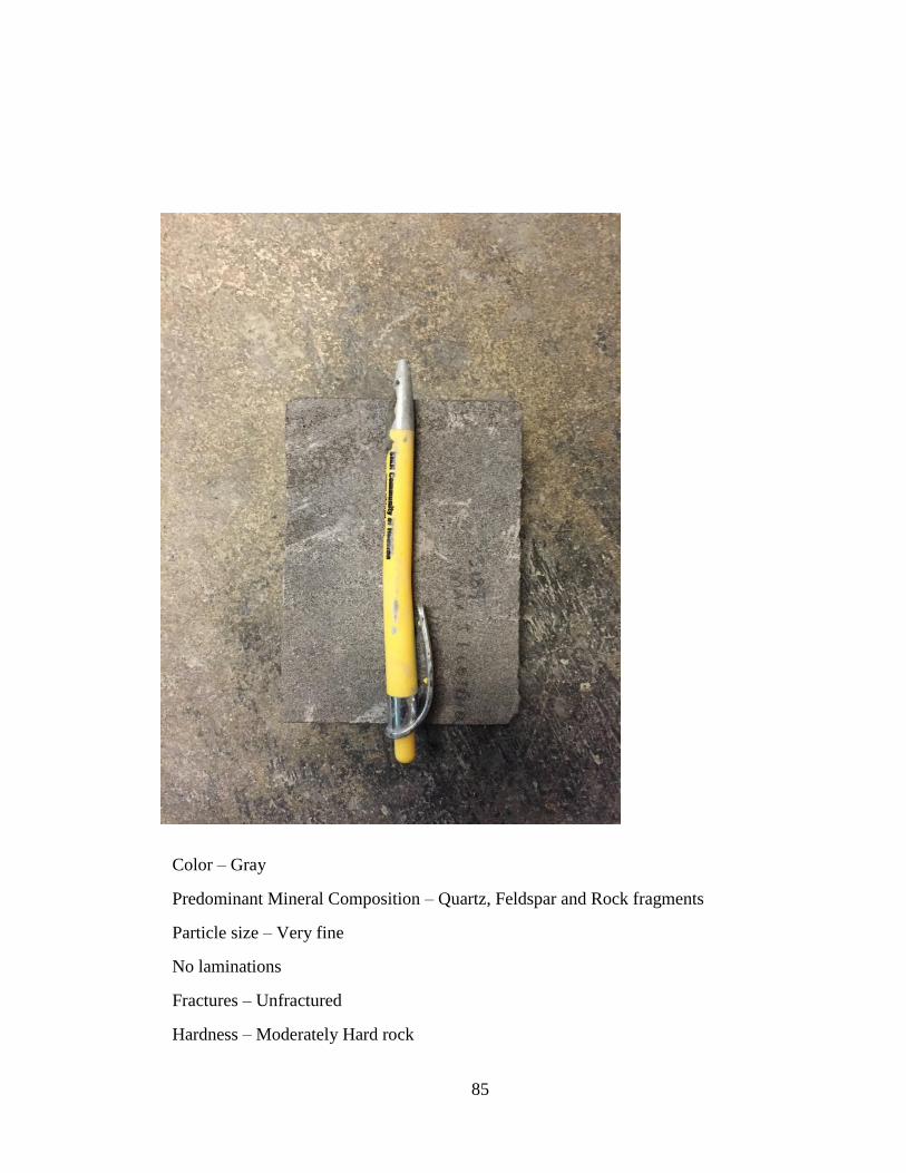
85
Color – Gray
Predominant Mineral Composition – Quartz, Feldspar and Rock fragments
Particle size – Very fine
No laminations
Fractures – Unfractured
Hardness – Moderately Hard rock

86
Color – Light yellow
Predominant Mineral Composition – Quartz, Feldspar and Rock fragments
Particle size – Very fine
Thinly laminated
Fractures – Unfractured
Hardness – Moderately Hard rock

87
Color – Gray
Predominant Mineral Composition – Quartz, Feldspar and Rock fragments
Particle size – Very fine
No laminations
Fractures – Unfractured
Hardness – Moderately Hard rock

88
Color – Gray
Predominant Mineral Composition – Quartz, Feldspar and Rock fragments
Particle size – Very fine
No laminations
Fractures – Unfractured
Hardness – Moderately Hard rock

89
Color – Gray
Predominant Mineral Composition – Quartz, Feldspar and Rock fragments
Particle size – Very fine
No laminations
Fractures – Unfractured
Hardness – Moderately Hard rock

90
VITA
Pawan Kakarla graduated from Narayana Junior College in Vijayawada, Andhra
Pradesh, India, in May of 2008. Pawan attended Indian Institute of Technology, Roorkee,
India from the Fall of 2008 to the Spring of 2013, where he graduated with an Integrated
M. Tech in Geological Technology. After receiving his master’s degree, Pawan began
working on his M.S. in Geology at Stephen F. Austin State University in August of 2014
where he graduated in August of 2016.
Permanent Address:
118, Sitapuram Colony, Poranki
Vijayawada, Andhra Pradesh, 521137,
India
Style: Geological Society of America
This thesis was typed by Pawan Kakarla