Geotechnical characterization of the upper Pleistocene–Holocene alluvial deposits of Roma (Italy) by means of multivariate geostatistics: Cross-validation results Giuseppe Raspa

a, Massimiliano Moscatelli

b, Francesco Stigliano

b, Antonio Patera

b,1, Fabrizio Marconi

b,

Daiane Folle a,d

, Roberto Vallone b, Marco Mancini

b, Gian Paolo Cavinato

b, Salvatore Milli

c,b, João Felipe

Coimbra Leite Costa d

a) Dipartimento di Ingegneria Chimica, dei Materiali, delle Materie Prime e Metallurgia, Università di Roma “La Sapienza”, Via Eudossiana 18, Roma, 00185, Italia

b) CNR-IGAG, Istituto di Geologia Ambientale e Geoingegneria, Via Bolognola 7, Roma, 00138, Italia c) Dipartimento di Scienze della Terra, Università di Roma “La Sapienza”, Piazzale Aldo Moro 5, Roma, 00185, Italiad

d) Departamento de Engenharia de Minas, Universidade Federal do Rio Grande do Sul, Av. Bento Gonçalves 9500, Porto Alegre, RS, 91501-970, Brasile 1) Present address: Istituto Nazionale di Geofisica e Vulcanologia, Sezione di Sismologia e Tettonofisica, Via di Vigna Murata 605, Roma, 00143, Italia

1) Introduction High levels of geohazard often involve urban areas with high anthropic pressure. Land subsidence and differential settlements in Venezia, Bangkok, Mexico City, and New Orleans (Burkett et al., 2003; Ovando-Shelley et al., 2003; Carbognin et al., 2004; Phien-wej et al., 2006), the collapse of underground caves and natural cavities in Mexico City and Napoli (Evangelista, 1991; Antonio-Carpio et al., 2004), and landslides in Hong Kong, Sao Paulo, and Taiwan (Au, 1998; Canil et al., 2004; Chang et al., 2005) are just some examples of natural disasters affecting urban areas. Public administrations, Civil Protection agencies, and research institutions are continuously involved in managing environmental hazards and planning future developments of urban areas, which both require in-depth knowledge of the subsoil. This knowledge is mainly based on accurate modelling of the physical and mechanical parameters, by means of both deterministic and probabilistic approaches. Nevertheless, the spatial distribution of geotechnical properties in natural soil is difficult to predict just deterministically, especially when sampling interests a very scarce portion of the total volume of soil (Jones et al., 2002; Parsons and Frost, 2002). Probabilistic methods, used along with conventional geotechnical applications, allow for quantifying uncertainty in assessing hazard mitigation measures and in designing projects to compensate for risks (Vannucchi, 1985; Lacasse and Nadim, 1996; Fenton, 1996, Parsons and Frost, 2002; Hack et al., 2006). Three primary sources of uncertainty are involved in geotechnical modelling: inherent soil variability, measurement error, and transformation uncertainty (Jones et al., 2002; Bourdeau and Amundaray, 2005; El Gonnouni et al., 2005). Apart from measurement error and transformation uncertainty, numerous papers have documented the uncertainty related to inherent variability of soil (e.g., Terzaghi, 1955; Haldar and Tang, 1979; Haldar and Miller, 1984a,b; Phoon and Kulhawy, 1996, 1999a). Other papers have quantified the spatial variability of physical and mechanical soil properties (e.g., Souliè et al., 1990; Nobre and Sykes, 1992; Jaksa et al., 1993; Liu et al., 1993; Jaksa, 1995; DeGroot, 1996; Jaksa et al.,1997; Popescu et al.,1997; Phoonand Kulhawy,1999b; Fenton and Griffiths, 2002; Baise and Higgins, 2003; Phoon et al., 2004; Dawson and Baise, 2005; El Gonnouni et al., 2005; Liu and Chen, 2006; Lenz and Baise, 2007; Sitharam and Samui,

2007). These works generally focus on geotechnical design, whereas hazard assessment is normally confined to seismic-related hazards. As a matter of fact, very little work has been done to specifically address geohazard assessment, especially in urban areas, where the effects of catastrophic events are often amplified because of ineffective land management. For its part, the Istituto di Geologia Ambientale e Geoingegneria (the hereafter IGAG) of the Italian Consiglio Nazionale delle Ricerche (the hereafter CNR) is coordinating a multidisciplinary research group to develop an integrated model of the subsoil of Roma aimed at the geohazard assessment of the city. The city of Roma has experienced a complex urban growth since its foundation. The challenge for the future will be the proper management, conservation, and development of the city, which suffers from some of the geohazards affecting other urban areas in the world. To date, the knowledge of the geological environment of Roma and of the surrounding Roman Basin have been based on published monographies and geological surveys (Ventriglia, 1971; Funiciello, 1995; Ventriglia, 2002; Funiciello and Giordano, 2005), and many research papers (e.g., Ambrosetti and Bonadonna, 1967; Bonadonna, 1968; Conato et al., 1980; Milli, 1992, 1994; Amanti et al., 1995; Bellotti et al., 1995; Boschi et al., 1995; Faccenna et al., 1995; Fäh et al., 1995; Marra and Rosa, 1995; Carboni and Iorio, 1997; Milli, 1997; Marra et al., 1998; Bozzano et al., 2000; Florindo et al., 2007). The stratigraphic framework of the Roman Basin is generally well defined except for the upper Pleistocene–Holocene alluvial deposits, mainly related to the Tevere and Aniene rivers (Fig. 1). It is noteworthy that these deposits occupy a sizable and significant part of the city, this unit being the foundation for many monuments, historical neighborhoods, and archaeological areas, and the main host of the present and future subway lines. This setting is particularly important for earthquake damage within the urban area, which has been shown to worsen in correspondence to the alluvial plain, where the strongest ground-motion amplification occurs because of the seismic impedance ratio between alluvial deposits and seismic bedrock (Ambrosini et al., 1986; Rovelli et al., 1994; Cifelli et al., 1999, 2000; Panza et al., 2000, 2001; Olsen et al., 2006; Bozzano et al., 2008). The model of the subsoil of Roma consists of the integration and analysis of the main available geological and geotechnical data: stratigraphy, lithology and texture, physical and mechanical properties, and hydrogeology. Information from more than 6000 boreholes and measured stratigraphic logs, geological maps, and in situ tests were homogenized, classified, and archived in a database thus far. Geological information retrieved from the database was interpreted and encoded to reconstruct the stratigraphic framework of the Roman Basin. Attention was specifically focused on the upper Pleistocene– Holocene alluvial deposits, which have suffered from the most significant geohazards in the study area. Information from more than 2000 boreholes penetrating these deposits is currently used to model their lithologic/textural associations. In this paper, we describe an attempt to evaluate the spatial variability of geotechnical parameters recorded in the alluvial deposits related to Tevere and Aniene rivers and to their tributaries (283 boreholes with a set of 719 samples), applying a probabilistic approach. In particular, techniques of multivariate statistics and geostatistics (i.e., Principal Component Analysis, multiple linear regression, kriging, and cokriging) are combined and compared to evaluate the estimation methods of the mechanical parameters, with special reference to the drained friction angle from direct shear test (φ′). The possibility of using granulometries as auxiliary variables to improve the estimation of φ′ is also tested and discussed. 2) Dataset Interpreted geological and geotechnical data of the subsoil of Roma were collected from public administrations and private companies. The collected information was classified and filtered according to specific criteria before being archived in the geodatabase, i.e., selecting boreholes with a reliable location, a

detailed lithologic description, and, possibly, with laboratory geotechnical tests. Information from more than 6000 wells, including continuous coring vertical boreholes and water wells (vintages from 1980s to 2000s), together with detailed geological maps, measured stratigraphic logs, and geotechnical in situ tests were homogenized and archived in an ESRI personal geodatabase managed by ArcGIS® (ESRI, Inc.). Approximately 3000 boreholes and stratigraphic logs were encoded and retrieved from the database in order to reconstruct the stratigraphic, structural, and depositional setting of the study area. More than 2000 of the archived and encoded boreholes cross the upper Pleistocene–Holocene alluvial deposits, which are related to the Tevere and Aniene rivers and to their tributaries. For this case study, only geotechnical boreholes with geotechnical information penetrating these deposits were selected (Fig. 1). The set includes 283 boreholes and 719 samples (Fig. 2). Two hundred and six of the selected boreholes, more than 70% of the total, have a TD (Total Depth, the final depth reached from land surface) between 20 m and 50 m. The TVDSS (Total Vertical Depth Subsea, the vertical depth reached from the mean sea level reference) is between −20 m and −40 m for 127 boreholes, 45% of the total. The distribution of the samples with the elevation is not uniform, with 269 samples (approximately 37%) between 0 m and 10 m a.s.l. and just 76 samples (approximately 11%) below −20 m a.s.l. The selected samples have a set of geotechnical information comprising the most relevant 13 physical properties — total unit weight (γn), unit weight of soil particles (γs), natural water content (wn), liquid limit (wl), plastic limit (wp), plasticity index (Ip), consistency index (Ic), clay activity (A), void ratio (e0), gravel percentage (Gravel%), sand percentage (Sand%), silt percentage (Silt %), clay percentage (Clay%) — and 2 mechanical parameters — drained friction angle from direct shear test with the Casagrande apparatus (φ′), and drained cohesion from direct shear test with the Casagrande apparatus (c′). The geotechnical information is not homogeneously distributed among the samples (Fig. 3). The complete set of geotechnical information is available for just 51 samples. Almost all the samples (702 out of 719) have the textural information (i.e., Gravel%, Sand%, Silt%, and Clay%; Txt in Fig. 3), besides the γn (709 samples), wn (709 samples), and γs (664 samples) values. There are 154 samples with all the physical properties, while the mechanical parameters φ′ and c′ are contemporaneously available for 312 samples (Fig. 3). 3) Stratigraphic and depositional setting The city of Roma is located on the Tyrrhenian margin of the Italian peninsula (Fig. 1), at the convergence between the central and northern Apennines. The substrate of the city originates from the almost continuous superimposition of Pliocene–Quaternary marine and continental sedimentary deposits (Funiciello, 1995; Milli, 1997; Funiciello and Giordano, 2005), which are interfingered with products of the Sabatini Mts. and Alban Hills Volcanic Districts since the middle Pleistocene. In historic times, the damming of water courses, land reclamation, and quarry activities modified the original morphology of the Roman countryside, which is at present hidden by a thick blanket that has recorded the almost continuous anthropic activity of the last 3000 years. The resulting stratigraphic setting is so complex that it could hardly be applied for spatial modelling of the recognized units. Because of this complexity, a simplified stratigraphic chart was synthesized for the purpose of this study (Fig. 4), integrating available geological information (i.e., boreholes, stratigraphic sections, geological maps) and literature data. Seven hundred boreholes and stratigraphic logs were selected out of the 3000. Using this information and following the stratigraphic chart of Fig. 4, more than 90 crosssections were produced. Eight informal lithostratigraphic units, roughly corresponding to unconformity-bounded stratigraphic units, were recognized in the subsoil of Roma (Figs. 4 and 5), in accordance with the work of previous authors (Funiciello, 1995; Milli, 1997, and references therein): Monte Vaticano (Pliocene), Monte Mario (early Pleistocene), Ponte Galeria–Paleotevere (middle Pleistocene), Sabatini and Alban Hills

Volcanic Deposits and Ancient Alluvial Deposits (middle Pleistocene), Terraced Alluvial Deposits (middle-late Pleistocene), Recent Alluvial Deposits (from late Pleistocene to Holocene), and Anthropic Backfill (Historic time). An integrated analysis of correlation panels, geological maps, and isopach and isobath maps of the recognized units has allowed us to mark the tectonic-sedimentary evolution of the Roman Basin in the last 2 Ma, with special regard to the Recent Alluvial Deposits of the Tevere and Aniene rivers (Cavarretta et al., 2005a). This unit refers to the last glacial–interglacial cycle of post-Tyrrhenian age (approximately the last 120 ka), and in the study area it almost completely refers to the last 18 ka (Bellotti et al., 1994, 1995; Chiocci and Milli, 1995; Milli, 1997). The boreholes crossing the alluvial deposits were correlated to define the stratigraphic architecture and the internal lithologic/textural distribution of this unit. Three superimposed facies associations, the hereafter FA, were distinguished in the alluvial deposits of the Tevere and Aniene valleys (Fig. 5): FA 1) composed of pebbles and sandy pebbles, with an erosive lower boundary ranging from north to south from −30 m to −60 m below the present sea level, and thickness increasing from 5–10 m to 20–25 m in the same direction; FA 2) composed of organic rich clays with frequent lenses of sands and subordinate lenses of pebbles, with a thickness variable between 20 m and 40 m from north to south; FA 3) composed of silty clays with lenses of sands, with nearly constant thickness of 20–25 m along the investigated alluvial plains. The Recent Alluvial Deposits, with their internal facies associations, belong to the Tiber Depositional Sequence (Bellotti et al., 1994, 1995), also known as PG9 depositional sequence (Milli, 1997). The PG9 is an incomplete fourth-order depositional sequence (Fig. 4), still evolving in the marine and continental sectors of the Tyrrhenian margin, whose sequence boundary (SB) is represented by an erosional surface curved into the Plio-Pleistocene substratum during the last glacio-eustatic sea level fall (between 120 ka and 18 ka) (Milli, 1997; Amorosi and Milli, 2001). The sequence consists of coeval and genetically related depositional systems, called systems tracts, recording the close interaction between relative sea level changes and sediment supply (Posamentier and Allen, 1999). The PG9 sequence, like other depositional sequences, comprises three systems tracts: the lowstand systems tract (LST), the transgressive systems tract (TST), and the highstand systems tract (HST), although only the TST and HST seem to be recorded in the study area. In particular, FAs 1 and 2 belong to the fluvial systems of the TST, and internally show a retrogradational to aggradational stacking pattern formed during the last glacio-eustatic sea level rise (Bellotti et al., 1995; Milli, 1997; Amorosi and Milli, 2001). Gravel, sandy gravel, and sandy fining-upward facies sequences constitute the building block of these two units (Fig. 5). The FA 2 of the TST is separated from the overlaying FA 3, which belongs to the HST, through the maximum flooding surface (MFS in Fig. 5). In the specific case of the Tevere River, the MFS is dated approximately 5–6ka(Amorosi and Milli, 2001), when the shoreline was at its maximum landward position. The deposits referable to FA 3 show a typical aggradational to progradational stacking pattern, and are mainly constituted of flood plain muddy sediments with intercalation of sandy fluvial bodies (Fig. 5). 4) Geotechnical characterization of the Recent Alluvial Deposits The stratigraphic and sedimentological complexity of the Recent Alluvial Deposits makes their geological and geotechnical characterization a difficult process. Recent studies on the upper Pleistocene–Holocenic alluvial deposits of the Tevere River and its tributaries have allowed for defining geotechnical units with homogeneous geomechanical behaviour. The characterization of these units was carried out through the analysis of the lithological, physical, and mechanical characteristics retrieved from stratigraphic reports, and laboratory and in situ tests. Such geotechnical characterization refers to local geological models (Corazza et al., 1999; Bozzano et al., 2000) or to generalized models defined through representative stratigraphic logs for each water stream (Campolunghi

et al., 2007). In both cases, the proposed models are deterministic and they are applied to extrapolate results achieved for a 1D or 2D space to a 3D space. Deterministic methods are suitable for local reconstructions and for areas with high density data. Nevertheless, these methods are not very appropriate when scarcity and spatial distribution of the gathered samples do not allow for characterizing the volumes which they are collected from. Furthermore, deterministic methodologies require the elaboration of a countless number of cross-sections and synthetic stratigraphic logs for a 3D space reconstruction. A broader probabilistic approach could be worthwhile when managing subsoil datasets (Souliè et al., 1990; Rosenbaum et al., 1997; Nathanail and Rosenbaum, 1998; Parsons and Frost, 2002), especially in urban areas, where a comprehensive geohazard overview is as important as the detailed knowledge of local criticalities (Van der Merwe,1997; Glassey and Morrison, 1998; Denis et al., 2000; Duman et al., 2005; El Gonnouni et al., 2005; Jones et al., 2005; Bourgine et al., 2006). As a matter of fact, we followed an integrated probabilistic approach for modelling the subsoil of Roma (Cavarretta et al., 2005b; Folle et al., 2006). Three-dimensional space reconstruction of sedimentary bodies is currently performed by means of physicalstratigraphic and geostatistical methodologies, and with the support of the earthVision® application of Dynamic Graphics, Inc. The relationships between the physical and mechanical parameters of the samples are also investigated using statistics and multivariate geostatistics. The last step of the research would be the definition and characterization of geotechnical units, relating the physical/mechanical characteristics to the lithologic/textural properties of the sedimentary bodies. This geotechnical modelling is beyond the scope of this paper, which mainly focuses on the evaluation of the methods to estimate the geotechnical parameters. 4.1. Physical and mechanical features of the alluvial deposits Physical and mechanical properties of the Recent Alluvial Deposits are analyzed in the following before performing further investigations. The main physical features of the studied samples are summarized in Figs. 6, 7, and 8. Grain size data of the 702 samples with textural information are plotted on the triangular graphs of Fig. 6A (after US Bureau of Soils; Rose, 1924). Samples show a very large variability ranging from sand to clay, with most of them classifiable as clay and silty clay (Fig. 6A). The 51 samples with a complete set of geotechnical information are mainly clay and silty clay, and subordinately silty clay loam (Fig. 6B). The plasticity condition of the Recent Alluvial Deposits is highlighted by the plasticity chart of Fig. 7, where the samples refer to the investigated valleys (for the location, see Fig. 1). The plasticity chart shows high plasticity of the organic deposits from the Tevere, Aniene, and S. Agnese areas, and especially from the Caffarella tributary area (Fig. 7). The activity chart of Fig. 8 shows inactivity to normal activity for most of the samples. High activity values (A>1.25) mainly refer to samples from the S. Agnese area, and subordinately to samples from the Tevere, Aniene, and Caffarella area (Fig. 8). This distribution is consistent with the activity values shown by Campolunghi et al. (2007). A preliminary analysis of the geotechnical information was carried out to investigate the relationships between lithologic/textural and geomechanical properties. The lithologic/textural data of selected boreholes was encoded to define representative classes and associations. Within the alluvial deposits, 17 lithologic/textural classes were detected and were grouped into 5 main associations (Fig. 9). The scatterplots of Fig. 10 show the trend of the phase properties (γn, wn, and e0) and of the drained friction angle (φ′) versus TD, as a function of the lithologic/textural classes. The volcanoclastic and organic fractions clearly influence the γn, wn, and e0 values of the sandy (AR2v, Fig. 10A and D) and silty (AR3v and AR3t, Fig. 10B and E) deposits, while the clayey deposits show a trend for wn and e0 with TD (Fig. 10F and I). The drained friction angle φ′ is not clearly correlated to the lithologic/ textural classes, except for values less than 25°, which are typical of silty classes (AR2l and AR3; Fig. 10j and k, respectively) and organic clays (AR4t, Fig. 10l).

The physical/mechanical parameters of the lithologic/textural classes only show a faint correlation with TD. The observed trends are again connected to the volcanoclastic (Fig. 10A, B, D, E, G) and organic (Fig. 10C, F, I) fractions, whose abundance is in turn related to the stratigraphic and structural setting of the alluvial deposits. Indeed, volcanoclastic alluvial deposits mainly fill the valleys of the Tevere left-bank tributaries, which were carved into the Pleistocene volcanic deposits of the Alban Hills, and were filled during the trangressive (TST) and highstand (HST) phases of the PG9 sequence. On the other hand, the organic fraction is diffused in the entire valley fill, especially in the clay deposits of the TST (FA 2, Fig. 5). It is noteworthy that samples coming from clayey levels (AR4 and AR4s) show a peak in φ′ values at TD between 10 m and 20 m (Fig. 10L). These values are recorded in correspondence to the MFS (Fig. 5), and are probably related to overconsolidation processes due to vertical oscillations of the groundwater table (see also Corazza et al., 1999; Bozzano et al., 2000). Such vertical fluctuations seem to be induced, in the lower reaches of the river systems and close to the coast line, by the quasi-still stand of the sea level at the time of the MFS (see Posamentier and Allen, 1999). With the exception of a few cases, these graphs do not highlight any clear correlation between the lithologic/textural characteristics and the physical/mechanical properties of the samples. The lack of a clear relationship between lithologies/textures and geotechnical properties is in great measure due to the different scale of observation used for the lithologic/textural description and for the geotechnical parameterization. In a continuous coring borehole, indeed, the lithologic/textural description is continuous. It is an interpretative and subjective process easily influenced by the training and the preconceived ideas of the surveyor. On the other hand, the sampling of a continuous coring borehole is punctual, and the geotechnical parameters are retrieved by laboratory tests. This inconsistency shows up when dealing with subsoil information and is generally underestimated when modelling geological and geotechnical data. Moreover, there is not even a clear correlation between the physical/ mechanical parameters (γn, wn, e0,and φ′) of the samples and their location (Fig. 11), as well as for the lithologic/textural properties. A weak correlation shows up only for the samples of the Caffarella and Cecchignola water streams, left-bank tributaries of the Tevere River (Fig. 1), and of the S. Agnese water stream, left-bank tributary of the Aniene River (Fig. 1). In particular, the samples coming from the Caffarella and Cecchignola tributaries have low γn values and high wn values (Fig. 11Aand B), probably as a consequence of their lithologic/textural signature (the volcanic component is prevalent here). The γn and wn values of the Caffarella tributary are not directly related to the e0 values, probably due to the abundant organic fraction (see Fig. 7). The physical/mechanical parameters change with TD more for the tributaries rather than for the main trunks (Fig. 11). Geometric and stratigraphic constraints clearly influence the vertical distribution of these parameters. As a matter of fact, the depth of sampling in the tributaries is directly related to the total thickness of the valley filling. This thickness ranges between 40 m and 60 m for the Tevere and Aniene rivers, and is not greater than 30 m for the tributaries. In conclusion, the preliminary study of the physical/mechanical parameters shown in Figs. 10 and 11 is obviously not comprehensive of the total variability of the studied samples. This variability is hidden in the complex relationships linking the entire set of physical/mechanical properties. Therefore, because of the numerous involved variables, the spatial extent of the geological bodies, and the complex relationships existing among the physical/mechanical properties, multivariate statistics and geostatistics seem to be the most suitable tools to investigate the relationships among the geotechnical parameters. These methodologies were applied to the samples of the Recent Alluvial Deposits, and the results of this application are accounted for in the following paragraphs.

5) Methods Geostatistical analysis performed in this work was aimed to define the best estimation conditions of the mechanical parameters, taking into account all the available information described in sections two and four. Three questions were particularly faced in our analysis:

1) if and how punctual estimation of mechanical parameters can be improved by using auxiliary variables, such as the physical properties; 2) which are the auxiliary variables to use in estimation, considering that there are a lot of variables, and gaps of information are numerous as well; 3) which is the estimation method to use with respect to its efficacy and operability.

Kriging and cokriging are geostatistical methods that use spatial correlation to estimate a target variable at a defined point: kriging by using measures of the target variable near the estimation points, and cokriging also by using auxiliary variables (Goovaerts, 1997; Deutsch and Journel, 1998; Chilès and Delfiner, 1999; Wackernagel, 2003). The first question was handled by doing a cross-validation of φ′ (see paragraph 6.2) with both kriging and cokriging, at first using the 13 physical parameters as auxiliary variables. Cross-validation method is often used in geostatistics to compare both different estimation conditions and different estimators. This method is performed by making estimation on the points where variable is already known and comparing results with measures by means of defined statistics. Since performing a cokriging with 13 variables was not really feasible, physical parameters were replaced with the principal factors arising from a Principal Component Analysis (Härdle and Simar, 2007). Only 15% of the total variability was lost as a consequence of this substitution (see section six), thanks to a redundancy of information. Counting on the encouraging cross-validation performed using the physical information synthesized in the factors of Principal Component Analysis, a new cross-validation was carried out using the most abundant physical variables (i.e., granulometries) as auxiliary information for cokriging. Considering the low amount of information available to reconstruct mechanical properties with respect to the very large volume of interest, a small contribution of spatial correlation to the estimation was expected. Therefore, multiple linear regression (Saporta, 1990; Härdle and Simar, 2007) was also tested as estimator through crossvalidation. This method uses the only auxiliary information available on the estimation point, taking advantage of the global correlations among the variables. Before describing the results of our analysis, methods previously introduced are described below. Principal Component Analysis (Härdle and Simar, 2007). This is a method of multivariate analysis that linearly transforms a set of numerical variables, usually correlated, into a set of as many independent variables, with mean 0 and variance 1, called factors, and generated in order to progressively describe the maximum part of original total variability. Very often factors, which are influenced by groups of variables, represent underlying physical phenomena that can be highlighted because of this method. Owing to the redundancy of information related to correlations among the variables, few factors are generally adequate to account for the original variability. Coordinates of each sample with respect to the factors can be calculated to allow a subset of the original information to be used in any requested application (in our case, cokriging). Sample points can also be visualized by means of their projections on planes defined by pairs of factors. Due to the linear transformation, an original variable can be expressed as a linear combination of factors. If the variable is standardized (this is our case), then coefficients of the linear combination correspond to the correlation coefficients between the variable and the factors. Each standardized variable is consequently represented in the space of factors by a vector of range 1 and is placed on the hyper sphere of range 1. Taking into consideration two variables, their correlation coefficient represents the cosine of the angle

formed by the correspondent vectors, so that two well-correlated variables are close on the hyper sphere. Variable-points disposed on the hyper sphere can be projected on the factors plane for a prompt graphic representation of the relations, both among the variables and among variables and factors. Two variable-points that are close on the hyper sphere are also close on all the planes, but not vice versa. Variables measured on the sample-point but not used for Principal Component Analysis (i.e., supplementary variables) can be localized on the hyper sphere as well, and consequently projected on planes of factors. Multiple linear regression (Saporta, 1990; Härdle and Simar, 2007). Given a target variable 0Z (in the

present case, φ′; see paragraph 6.2) and a set of p auxiliary variables ( )1,iZ i p= (in the present case, the 13

physical parameters), all measured on n sample points ( )1,x nα α = , the multiple linear regression of the

main variable at a given point x0 on auxiliary variables at the same location is given by a linear combination of the residuals:

* * *0 0 0 0

1

( ) [ ( ) ]=

= + −∑p

i i ii

z x m a z x m (1)

where { }*im is the vector of the means of variables, and { }ia is the vector of the coefficients weighting the

single variables. This vector is calculated by minimizing the sum of square difference between *0 ( )az x and

its own measure 0 ( )az x for all the n measured points. The minimization process uses the matrix

variance/covariance of the p variables, and the vector of covariances between the target variable and each of the auxiliary variables. Ordinary kriging (Goovaerts, 1997; Deutsch and Journel, 1998; Chilès and Delfiner, 1999; Wackernagel, 2003). This is the most popular geostatistical method. It is used to estimate the value of a variable 0Z in a

point 0x of the space, using a set of values of the same parameter measured on 0n near points

( )01,x nα α = . This method consists of a linear combination of the measures:

0* 00 0 0

1

( ) ( )n

z x z xα αα

λ=

= ∑ (2)

where the vector of the coefficients { }0αλ is calculated in order to have a correct estimator, and to minimize

the difference between the unknown value on the estimation point and the kriged value on the same point. Minimization takes into account the spatial variability of the parameter expressed by the variogram function 0 ( )hγ , which is the semivariance of the parameter increment with respect to distance h:

[ ]0 0 02 ( ) var ( ) ( )h z x h z xγ = + − .

Variogram function is adjusted on experimental variograms by means of a fitting operation. Ordinary kriging is characterized by a measure of its accuracy, which is the estimation error variance. This is useful to define estimation uncertainty and to outline areas that need a supplemental sampling. Ordinary cokriging (Goovaerts, 1997; Deutsch and Journel, 1998; Chilès and Delfiner, 1999; Wackernagel, 2003). This is a correct linear estimator as ordinary kriging. It is used to estimate the value of a variable 0Z

in a point 0x of the space, by means both of values of the same parameter measured on points near to 0x and

of measures of other parameters ( )1,iZ i p= spatially correlated to 0Z .

Indicating with ( )1,in i p= the number of sampled points near 0x , and considering the 1p + parameters,

the estimator is:

*0 0

0 1

( ) ( )inp

ii

i

z x z xα αα

λ= =

= ∑ ∑ . (3)

A minimization procedure similar to ordinary kriging is used to determine the matrix of coefficients { }iαλ ,

which introduces spatial variability of all parameters by means of the set of direct and cross variograms

{ }( )i j hγ . The generic cross variogram between parameter iZ and jZ is defined as the semicovariance of

the parameter pair increments:

2 ( ) cov ( ( ) ( )), ( ( ) ( ))ij i i j jh z x h z x z x h z xγ ⎡ ⎤= + − + −⎣ ⎦ . (4)

Variograms set is introduced in the estimation by means of a model that guarantees the mathematical coherence. The most frequently used model is the linear corregionalization model, according to which the generic cross variogram of each structure with variability u (nugget, low or great scale) ( )u

ij hγ has a sill uijb that depends on the specific parameter pair, and a variogram ( )ub h with sill 1 that is the same for all the

parameter pairs: ( ) ( )u u

ij ij uh b g hγ = . (5)

Model adjustment is realized by means of a fitting operation on the experimental variograms, respecting the

condition that matrixes { }uijb are defined positive.

6) Results and discussions 6.1. Principal Component Analysis of the geotechnical parameters The 51 samples of the Recent Alluvial Deposits with a complete set of geotechnical information were analyzed to characterize the 13 most relevant physical properties and 2 mechanical parameters. Principal Component Analysis, the hereafter PCA, was the first step for subsequent geostatistical analysis. PCA was indeed applied both i) to highlight the relationships among the geotechnical parameters and ii) to synthesize all the auxiliary physical information available for cokriging application. PCA results provided in Table 1 show coordinates of the 13 active variables in respect to the axes of the first five factors. As exposed in the previous section, the coordinates in question are just the correlation coefficients among variables and factors. The last two rows of the Table 1 show coordinates of φ′ and c′ with respect to the same five factors; in this specific case, mechanical parameters are involved in the PCA as supplementary variables. Due to the redundancy of information related to correlations existing among the parameters, the first five factors of the PCA explain more than 85% of the total variability; specifically, the first two factors explain 53.70% of the total variability. The graphical display of the first two columns of Table 1 in the plot of Fig. 12 allow us to promptly clarify the meaning of the first two factors. With the exception of factor 3, which is fairly related to the variables, the other four factors are closely or very closely related to the variables (Table 1). Factor 1, which explains 29.15% of the total variability, is highly correlated to Ic (0.7434), γn (0.8337), wn (−0.9098), and e0 (−0.8723), and is likely controlled by the water content of the samples (saturation is assumed to be 100% for the studied alluvial deposits). Factor 1 is weakly correlated to φ′ (−0.1605) and c′ (0.2482). Factor 2, which explains 24.55% of the total variability, is correlated to Clay% (−0.8520), wl (−0.7822), and Ip (−0.7368), and is likely controlled by the amount and mineralogical composition of the clay component.

This factor is closely related to φ′ (0.7413), whereas it is weakly correlated to c′ (−0.3147). Factor 3 explains 14.14% of the total variability, and is fairly related to Sand% and γs (−0.4495 and −0.4364, respectively), in opposition to Silt% (0.5597), A (0.6070), and wl (0.5393). Factor 3 is weakly correlated to φ′ (−0.1444) and c′ (−0.1864). Factor 4, which explains 9.90% of the total variability, is closely correlated to wp (0.7460) and fairly related to γs (0.4246), Ip (−0.4033), Ic (0.4206), and A (−0.3992). This factor is moderately correlated to c′ (0.5211). Finally, Factor 5 explains 7.70% of the total variability, and is closely correlated to Gravel % (−0.7424), whereas it is weakly related to φ′ (−0.2178). 6.2 Cross-validation of estimation methods In the present work, attention was focused on drained friction angle φ’, which shows the most promising correlation to the physical parameters. A cross-validation analysis was performed to highlight the contribution of spatial correlation and auxiliary variables to the estimation of φ’. The 13 physical variables available for the 51 samples provided with the full set of geotechnical information were at first involved in estimation of φ’. Three estimators were compared: 1) multiple linear regression, which uses the values of auxiliary variables uniquely on the estimation points for estimation, taking advantage both of total reciprocal correlations among the variables and of correlations between each auxiliary variable and target variable; 2) ordinary kriging (the hereafter kriging), which uniquely uses the spatial correlation of the target variable for estimation; 3) ordinary cokriging (the hereafter cokriging), which uses the spatial correlation of both of target and auxiliary variables for estimation. Multiple linear regression, kriging, and cokriging were performed using ISATIS® from Geovariances. With the aim of making cokriging operative with all the available physical information, the 13 physical variables were synthesized by the first five factors of the PCA (Tab. 1). Given the limited number of available samples (i.e., 51 samples), a corregionalization model was achieved assuming a variogram model with one nugget component and two zonal spherical components:

( ) ( ) ( ) ( )nugget vert v hor hh h h hγ γ γ γ= + + , (6)

where vh is the projection of h on the vertical direction, and hh is the projection of h on the horizontal

plane. The ranges of vertical variogram ( vertγ ) and isotropic horizontal variogram ( horγ ) were varied by trial

and error to obtain the best estimations. Sill matrixes were automatically adjusted by the software when changing the ranges. Cokriging was performed by preserving auxiliary information on the estimation point, in order to compare results with multiple linear regression estimations. Besides scatterplots measures/estimations, the following parameters were used to compare cross-validation results: variance of cross-validation errors, correlation coefficient between estimated and measured values, and regression coefficient of measured versus estimated values. Cross-validation results, which are reported in Figure 13 and Table 2, can be summarized in the following points: 1) Multiple linear regression gives better results than kriging, suggesting that auxiliary information on the estimation point is more effective than spatial correlation of φ’. Nevertheless, kriging results are influenced by the great distance between samples and estimation points. 2) Cokriging, which takes into account both spatial correlation and auxiliary variables, provides the best estimations of φ’. Moreover, scatterplots (Fig. 13) show that multiple linear regression overestimates low values of φ’, while

overestimation does not occur with cokriging, despite information scarcity, because it uses the direct variable. Otherwise, kriging underestimates high values and overestimates low values of φ’, respectively. Cokriging estimation of φ’, performed with 51 samples, is essentially influenced by the second factor resulting from the PCA; besides φ’, this factor is mainly correlated to grain size, wl, and Ip. Considering both the good correlation between φ’, and the physical properties influencing Factor 2 and the abundance of their measures in the dataset (see Fig. 3), cokriging was again performed with the same dataset (i.e., 51 samples), trying different combinations of grain size, wl, and Ip as auxiliary information. Sand%+Gravel% - Clay% was proven to be the best combination of auxiliary variables. Cross-validation results of this combination are: variance of errors = 8.72, correlation coefficient between estimated and measured values = 0.74, regression coefficient of measured versus estimated values = 0.53. Apart from this last value, the other two statistics are slightly worst than values reported in Table 2. Another important outcome of these trials is the bad performance of the combination Sand%+Gravel% - Silt% - Clay%, in contrast with the expected results. Since previous results demonstrated that estimation of φ’ improves by using granulometries as auxiliary variables, a subsequent step of the study was the estimation of φ’, using the combination Sand%+Gravel% - Clay% from all the available information. Cokriging was realized by using textural parameters recorded on 702 samples, and estimating φ’ on 295 points (i.e., samples), where its own value was available. Coregionalization model was adjusted on the experimental variograms (Fig. 14), which were calculated with a lag size of 10 m on the vertical direction and 500 m on the horizontal plane. The first point of the experimental variograms was calculated with all the pairs having a maximum distance of half the lag size (Fig. 14). Experimental variograms show an anisotropic variability, which is typical of fluvial sedimentary successions: a small range in the vertical direction and a large range in the horizontal direction. The range is indeed related to dimensions of sedimentary bodies, which have a thickness of about 10 m, and a width ranging from 500 m to 2 000 m (see correlation panel of Fig. 5). The range of vertical variograms is about 10 m, consistent with the stratigraphic signature of the Tevere system and with literature (DeGroot, 1996; Phoon and Kulhawy, 1999b; Lenz and Baise, 2007). The range of horizontal variograms is quite variable, spanning from 400 m for Sand%+Gravel% - Clay% to 1 000 for φ’; these values are also consistent with sedimentary processes attributed to the Tevere system, and are coherent with literature (DeGroot, 1996; Lenz and Baise, 2007; Thompson et al., 2007). The variogram model fitted with the experimental variograms follows the scheme of equation (6), with one nugget component and two zonal spherical structures: a vertical structure with a range of 12 m (Fig.14b), and an isotropic horizontal structure with a range of 670 m (Fig.14a). Sill matrixes were automatically adjusted by the software through the conditional fitting of the experimental variograms. The horizontal range of 670 m was defined by doing a set of cross-validations of φ’, tentatively changing the range between 400 m and 1 000 m. The value giving the best cross-validation result was chosen as the proper range. The isotropic horizontal structure is consistent with geometries of the sedimentary bodies at the scale of the entire study area. We are dealing with meandering fluvial systems, where sedimentary bodies can be oriented in all directions. As a matter of fact, spatial variability of the depositional system would require a locally variable model, although such a complex model would generally involve a greater amount of data. A new cross-validation analysis was carried out with multiple linear regression, kriging, and cokriging for the set of 295 samples, using granulometries as auxiliary variables. Performance of the three estimators was confirmed by cross-validation results (Tab.3 and Fig. 15), which testified to the feasibility of using granulometries for prevision of φ’. Contribution of auxiliary variables and spatial correlations to the estimation was confirmed: variance of errors for cokriging decreased by about 40% compared to kriging, and by 20% compared to multiple linear regression. It is noteworthy that, unlike cokriging, multiple linear

regression and kriging still overestimate low values and underestimate high values of φ’. Although very encouraging for future applications, cross-validation results are not surprising. Coherent with the theory, cokriging would provide the best result. In fact, cross-validation has a more important meaning: results being coherent with the theory, input data are also coherent, and this allows us to use them for estimation of geotechnical parameters, even though they come from different laboratories and different vintages. Finally, it is important to say that to get in estimation the same good results of cross-validation, it is necessary for granulometries to be available at grid points. Nevertheless, this information is not directly available, and in the future it is expected that granulometries can be derived in an indirect way, i.e., from detailed stratigraphic and lithologic/textural 3D reconstructions. 6.3 The role of silt in conditioning drained friction angle Textural data improves the estimation of the mechanical parameters. However, not all the granulometric percentages seem to be useful in the same way. As argued in paragraph 6.2, cokriging was performed using Clay% and Sand%+Gravel% as auxiliary variables, and the use of Silt% results in a worsening of the estimation. This behaviour is probably due to the different contribution of the silty component to the shear strength, when silt is associated with finer (i.e., clay) or coarser (i.e., sand and gravel) material. Moreover, for the Recent Alluvial Deposits, where the percentage of fines is prevailing, the mechanical behaviour of the samples probably depends on the different contribution of the plastic and non-plastic fines to the shear strength. This behaviour has already been observed for mixed materials and natural soils examined with undrained triaxial tests (Georgiannou et al., 1990; Pitman et al., 1994; Zlatović and Ishihara, 1995; Thevanayagam and Mohan, 2000; Ni et al., 2004, 2006), even though the results of these tests are not directly comparable with those coming from direct shear tests. Attempts to integrate the percentage of silt in estimation of φ’ will be pursued in the future by retrieving its granulometric distribution from the granulometric curves. An attempt to integrate the silt will be alternatively carried out by means of non-linear geostatistics, to account for the role of silt in conditioning φ’ as a function of values taken by other variables. 7) Conclusions and future work The spatial variability of geotechnical parameters in the upper Pleistocene-Holocene alluvial deposits of Roma (Italy) by means of multivariate geostatistics have been analyzed in this paper. Physical and mechanical information from 719 samples of 283 boreholes penetrating the alluvial deposits was processed for the spatial reconstruction of the drained friction angle (φ’). Principal Component Analysis was applied to the dataset to highlight the relationships between the geotechnical parameters. Through cross-validation analysis, multiple linear regression, kriging, and cokriging were tested as estimators of φ’. Cross-validation demonstrates that cokriging, using the percentage of clay and the added percentages of sand and gravel as auxiliary variables, is the best estimator of φ’. Textural information improves the estimation of φ’, but not all the granulometric percentages seem to be useful in the same way. As a matter of fact, the use of silt (i.e., percentage of silt) results in a worsening of the estimation of φ’. This behaviour is probably due to the different contribution of the silty component to the shear strength, when silt is associated with finer (i.e., clay) or coarser (i.e., sand and gravel) material. Prevision of φ’ could still be improved by finding a way of integrating silt in cokriging: for instance, by retrieving its internal granulometric distribution from the granulometric curves. Nevertheless, estimation of φ’ is expected to worsen when extended to all the alluvial deposits, since granulometries are not always available on the prevision points. For this reason, future research will focus on improving the estimation by linking granulometries and lithologic/textural features of the soils, so that the

final geotechnical modelling will unavoidably pass for the spatial reconstruction of the lithologic/textural properties. A further future step of the research will be the integration of information from cone penetration tests (CPT) and geophysical tests. These tests, constrained by stratigraphy of tied boreholes, will probably allow for overcoming the scale issues by linking punctual observations to the physical/mechanical properties of the soils. Finally, the application of multivariate geostatistics using physical/mechanical parameters from laboratory tests demonstrates its validity for the preliminary geotechnical characterization of alluvial deposits. Results of this work will be a useful tool for developing a tough procedure aimed at modelling the geological-geotechnical properties of subsoil. Acknowledgements This research was supported by National Research Council of Italy (CNR) and Dipartimento della Protezione Civile (UrbiSIT Project, DPC-IGAG). Authors would like to thank L.Baise, G. Crosta, and an anonymous reviewer for their revisions of the original manuscript. Authors would also like to thank S. Martino, M. Scarapazzi, and S. Storoni Ridolfi for thir useful discussions. Authors are very grateful to M. Albano, L. Angeloni, R. De Santis, D. Lori, G. Quaglia, S. Severi, and M. Tempesta for their technical and administrative support. LithoTect® from Geo-Logic Systems, LLC, and earthVision® from Dynamic Graphics, Inc., were used for geological modelling. Data used for analysis was kindly provided by APAT Agenzia per la Protezione dell'Ambiente e per i Servizi Tecnici, Comune di Roma, Roma Metropolitane S.p.A., Italferr S.p.A., Geoplanning - Servizi per il territorio s.r.l., S.G.S. Studio Geotecnico Strutturale s.r.l., S.I.G. Studio Indagini Geotecniche s.n.c., and I.Ge.S. Ingegneria Geotecnica Strutturale s.n.c.

References

Amanti, M., Gisotti, G., Pecci, M., 1995. I dissesti a Roma. In: Funiciello, R. (Ed.), La geologia di Roma; il centro storico. Memorie Descrittive della Carta Geologica d’Italia 50, 219–248.

Ambrosetti, P., Bonadonna, F. P., 1967. Revisione dei dati sul Plio-Pleistocene di Roma. Atti Accademia Gioenia di Scienze Naturali 18, 33–72.

Ambrosini, S., Castenetto, S., Cevolani, F., Di Loreto, E., Funiciello, R., Liperi, L., Molin, D., 1986. Risposta sismica dell’area urbana di Roma in occasione del terremoto del Fucino del 13 gennaio 1915. Memorie della Società Geologica Italiana 35, 445–452.

Amorosi, A., Milli, S., 2001. Late Quaternary depositional architecture of Po and Tevere River deltas (Italy) and worldwide comparison with coeval deltaic successions. Sedimentary Geology 144 (3-4), 357–375.

Antonio-Carpio, R.G., Perez-Flores, M.A., Camargo-Guzman, D., Alanis-Alcantar, A., 2004. Use of resistivity measurements to detect urban caves in Mexico City and to assess the related hazard. Natural Hazards and Earth System Sciences 4, 541-547.

Au, S.W.C., 1998. Rain-induced slope instability in Hong Kong. Engineering Geology 51, 1–36. Baise, L.G., Higgins, R.B., 2003. Geostatistical methods in site characterization. In: Der Kiureghian, A.,

Madanat, S., Pestana, J.M. (Eds.). Applications of statistics and probability in civil engineering, Millpress, Rotterdam, 1195-1202.

Bellotti, P., Chiocchini, U., Castorina, F., Tolomeo, L., 1994. Le unità clastiche plio-pleistoceniche tra Monte Mario (città d Roma) e la costa tirrenica presso Focene: alcune osservazioni sulla stratigrafia sequenziale. Bollettino del Servizio Geologico Italiano 113, 3–24.

Bellotti, P., Milli, S., Tortora, P., Valeri, P., 1995. Physical stratigraphy and sedimentology of the late Pleistocene-Holocene Tiber Delta depositional sequence. Sedimentology 42 (4), 617–634.

Bonadonna, F., 1968. Studi sul Pleistocene del Lazio V. La biostratigrafia di Monte Mario e la “fauna malacologica mariana” di Cerulli-Irelli. Memorie della Società Geologica Italiana 7, 261–321.

Bourdeau, P.L., Amundaray, J.I., 2005. Non-parametric simulation of geotechnical variability. Géotechnique 55, 95-108.

Boschi, E., Caserta, A., Conti, C., Di Bona, M., Funiciello, R., Malagnini, L., Marra, F., Martines, G., Rovelli, A., Salvi, S., 1995. Resonance of subsurface sediments: an unforeseen complication for designers of roman columns. Bulletin of the Seismological Society of America 85 (1), 320–324.

Bourgine, B., Dominique, S., Marache, A., Thierry, P., 2006. Tools and methods for constructing 3D geological models in the urban environment: the case of Bordeaux. Proceedings of the 10th IAEG Congress, International Association for Engineering Geology, 6-10 September 2006, Nottingham, Paper n° 72.

Bozzano, F., Andreucci, A., Gaeta, M., Salucci, R., 2000. A geological model of the buried Tiber River valley beneath the historical centre of Rome. Bulletin of Engineering Geology and the Environment, 59, 1-21.

Bozzano, F., Caserta, A., Govoni, A., Marra, F., Martino S., 2008. Static and dynamic characterization of alluvial deposits in the Tiber River Valley: New data for assessing potential ground motion in the City of Rome. J. Geophys. Res. 113, B01303, doi:10.1029/2006JB004873.

Burkett, Virginia, R., Zikoski, D.B., Hart, D.A., 2003. Sea-level rise and subsidence: implications for flooding in New Orleans, Louisiana. In: U.S. Geological Survey Subsidence Interest Group Conference, Proceedings for the Technical Meeting, USGS Water Resources Division, Open File Report Series 03-308, 63-70.

Campolunghi, M. P., Capelli, G., Funiciello, R., Lanzini, M., 2007. Geotechnical studies for foundation settlement in Holocenic alluvial deposits in the City of Rome (Italy). Engineering Geology 89 (1-2), 9–35.

Canil, K., Macedo, E.S., Gramani, M.F., Almeida Filho, G.S., Yoshikawa, N.K., Mirandola, F.A., Viera, B.C., Baida, L.M.A., Augusto Filho, O., Shinohara, E.J., 2004. Mapeamento de risco em assentamentos precarios nas zonas sul e parte da oeste no municipio de Sao Paulo (SP). Hazard mapping in the western and southern urban areas of Sao Paulo City, Sao Paulo. Proceedings of the “Simposio brasileiro de Cartografia geotecnica e geoambiental”, 16-18 of November 2004, Sao Carlos, Brazil.

Carbognin, L., Teatini, P., Tosi, L., 2004. Eustacy and land subsidence in the Venice lagoon at the beginning of the new millennium. Journal of the Marine System 51, 345-353.

Carboni, M. G., Iorio, D., 1997. Nuovi dati sul Plio-Pleistocene marino del sottosuolo di Roma. Bollettino della Società Geologica Italiana 116, 435–451.

Cavarretta G., Cavinato G.P, Mancini M., Moscatelli M., Patera A., Stigliano F., Vallone R., Milli S., Garbin F., Storoni S., 2005a. Geological and geotechnical modelling of the City of Rome. Proceedings of GEOITALIA 2005 – V Forum Italiano di Scienze della Terra, 23-24 of September 2003, Spoleto.

Cavarretta, G., Cavinato, G., Mancini, M., Moscatelli, M., Patera, A., Raspa, G., Stigliano, F., Vallone, R., Folle, D., Garbin, F., Milli, S., Storoni Ridolfi, S., 2005b. I terreni di Roma sotto l’aspetto della geologia tecnica. In: Gisotti, G., Pazzagli, G.,Garbin, F. (Eds.). La IV dimensione - Lo spazio sotterraneo di Roma. Geologia dell’Ambiente, Supplemento 4/2005, 33–46.

Chang, M., Chiu, Y., Lin, S., Ke T., 2005. Preliminary study on the 2003 slope failure in Woo-wan-chai Area, Mt. Ali Road, Taiwan. Engineering Geology 80, 93–114.

Chilès, J.P., Delfiner, P., 1999. Geostatistics: modelling spatial uncertainty. Wiley, New York, 695 pp. Chiocci, F.L., Milli, S., 1995. Construction of a chronostratigraphic diagram for a high-frequency sequence:

the 20 ky B.P. to Present Tiber depositional sequence. Il Quaternario 8, 339-348. Cifelli, F., Donati, S., Funiciello, F., 1999. Distribution of effects in the urban area of Rome during the

October 14, 1997 Umbria Marche earthquake. Physics and Chemistry of the Earth 24 (6), 483–487. Cifelli, F., Donati, S., Funiciello, F., Tertulliani, A., 2000. High-density macroseismic survey in urban areas;

Part 2, Results for the City of Rome, Italy. Bulletin of the Seismological Society of America 90 (2), 298–311.

Conato, V., Esu, D., Malatesta, A., Zarlenga, F., 1980. New data on the Pleistocene of Rome. Quaternaria 22, 131–176.

Corazza, A., Lanzini, M., Rosa, C., Salucci, R., 1999. Caratteri stratigrafici, idrogeologici e geotecnici delle alluvioni tiberine nel settore del centro storico di Roma. Il Quaternario 12, 215–235.

Dawson K.M., Baise L.G., 2005. Three-dimensional liquefaction potential analysis using geostatistical interpolation. Soil Dyn. Earthq. Eng. 25, 369-381.

DeGroot, D. J., 1996. Analyzing spatial variability of in situ soil properties. In: Shackleford C.D., Nelson P.P., Roth M.J.S. (Eds.). Uncertainty in the Geologic Environment: From Theory to Practice. ASCE Geotechnical Special Publication No. 58, Madison, WI, 210-238.

Denis, A., Breysse, D., Cremoux, F., 2000. Traitements et analyse des mesures de diagraphies diffèrès pour la reconnaissance gèotechnique. Bulletin of Engineering Geology and the Environment 58, 309-319.

Deutsch, C.V., Journel, A.G., 1998. Geostatistical Software Library and User’s Guide. Oxford University Press, 369 pp.

Duman, T. Y., Can, T., Ulusay, R., Kecer, M., Emre, O., Ates, S., Gedik, I., 2005. A geohazard reconnaissance study based on geoscientific information for development needs of the western region of Istanbul (Turkey). Environmental Geology 48 (7), 871–888.

El Gonnouni, M., Riou, Y., Hicher, P. Y., 2005. Geostatistical method for analysing soil displacement from underground urban construction. Géotechnique 55, 171–182.

Evangelista, A., 1991. Cavità e dissesti nel sottosuolo dell’area napoletana. Proceedings of the congress “Rischi naturali e impatto antropico nell’area metropolitana napoletana”, Napoli.

Faccenna, C., Funiciello, R., Marra, F., 1995. Inquadramento geologico e strutturale dell’area romana. In: Funiciello, R. (Ed.), La geologia di Roma; il centro storico. Memorie Descrittive della Carta Geologica d’Italia 50, 31–47.

Fäh, D., Iodice, C., Suhadolc, P., Panza, G., 1995. Application of numerical simulations for a tentative seismic microzonation of the city of Rome. Annali di Geofisica 38, 607-616.

Fenton G.A. (Ed.), 1996. Probabilistic Methods in Geotechnical Engineering. Workshop presented at ASCE GeoLogan’97 Conference, Logan, Utah. July 15, 1997.

Fenton G.A., Griffiths D.V., 2002. Probabilistic Foundation Settlement on Spatially Random Soil. J. Geotech. and Geoenvir. Engrg. 128, 381-390.

Florindo, F., Karner, D.B., Marra, F., Renne, P.R., Roberts, A.P., Weaver R., 2007. Radioisotopic age constraints for Glacial Terminations IX and VII from aggradational sections of the Tiber River delta in Rome, Italy. Earth Planet. Sc. Lett. 256, 61-80.

Folle, D., Raspa, G., Mancini, M., Moscatelli, M., Patera, A., Stigliano, F. P., Vallone, R., Cavinato, G. P., Cavarretta, G., Milli, S., Garbin, F., Storoni Ridolfi, S., 2006. Geotechnical modeling of the subsoil of Rome (Italy) by means of multivariate geostatistics. Proceedings of the XI International Congress. International Association for Mathematical Geology, Liège, Belgium, 3-8 September 2006.

Funiciello, R. (Ed.), 1995. La geologia di Roma. Il centro storico. Memorie descrittive della Carta geologica d’Italia. Servizio Geologico d’Italia, 50, 550 pp.

Funiciello, R., Giordano, G. (Eds.), 2005. Carta Geologica del Comune di Roma, Vol. 1. CD-ROM. Università di Roma TRE-Comune di Roma-DDS Apat.

Georgiannou, V. N., Burland, J. B., Hight, D. W., 1990. The ungrained behaviour of clayey sands in triaxial compression and extension. Géotechnique 40 (3), 431–449.

Glassey, P., Morrison, B., 1998. Dunedian Urban Pilot Study – A Hazard Information System. Proceedings the 10th Colloquium of the Spatial Information Research Centre, University of Otago, New Zealand, 16-19 November 1998, 89-96.

Goovaerts, P., 1997. Geostatistics for Natural Resources Evaluation. Oxford University Press, 483 pp. Hack, R., Orlic, B., Ozmutlu, S., Zhu, S., Rengers, N., 2006. Three and more dimensional modelling in geo-

engineering. Bull. Eng. Geol. Env. 65, 143-153. Haldar, A., Miller, F. J., 1984a. Statistical estimation of cyclic strength of sand. J. Geotech. Engng. 110,

1785-1802. Haldar, A., Miller, F.J., 1984b. Statistical estimation of relative density. J. Geotech. Engng. 110, 525-530. Haldar, A., Tang, W. H., 1979. Probabilistic evaluation of liquefaction potential. J. Geotech. Engng. 105,

145-163. Härdle, W., Simar, L., 2007. Applied Multivariate Statistical Analysis. Second edition. Springer-Verlag

Berlin Heidelberg, 458 pp. Jaksa, M. B. (1995). The influence of spatial variability on the geotechnical design properties of a stiff,

overconsolidated clay. Ph.D thesis, University of Adelaide, Australia. Jaksa, M. B., Brooker, P. I., Kaggwa, W. S., 1997. Modeling the spatial variability of the undrained shear

strength of clay soil using geostatistics. In: Baafi E. Y., Schofield N. A., (Eds.). Geostatistics Wollongong ’96 Vol. 2, 1284-1295.

Jaksa, M. B., Kaggwa, W. S., Brooker, P. I., 1993. Geostatistical modelling of the spatial variation of the shear strength a stiff, overconsolidated clay. Proceedings of the conference on probabilistic methods in geotechnical engineering, Canberra, 185-194.

Jones A.L., Kramer S.L., Arduino P., 2002. Estimation of Uncertainty in Geotechnical Properties for Performance-Based Earthquake Engineering. PEER 2002/16, Pacific Earthquake Engineering Research Center, College of Engineering, University of California, Berkeley.

Jones, T., Middelmann, M., Corby, N. (Eds.), 2005. Natural hazard risk in Perth, Western Australia. Cities Project Perth - Main report. Australian Government, Geoscience Australia, 352 pp.

Lacasse, S., Nadim, F., _1996. Uncertainties in characterizing soil properties. In: Shackleford C.D., Nelson P.P., Roth M.J.S. (Eds.). Uncertainty in the Geologic Environment: From Theory to Practice. ASCE Geotechnical Special Publication No. 58, Madison, WI, 49–75.

Lenz J.A., Baise L.G., 2007. _Spatial variability of liquefaction potential in regional mapping using CPT and SPT data. Soil Dyn. Earthq. Eng. 27, 690-702.

Liu, B.L., Li, K.S, Lo, S.-C.R., 1993. Effect of variability on soil behaviour: a particulate approach. Proceedings of the conference on probabilistic methods in geotechnical engineering, Canberra, 201-205.

Liu, C.-N., Chen, C.-H., 2006. Mapping Liquefaction Potential Considering Spatial Correlations of CPT Measurements. J. Geotech. and Geoenvir. Engrg. 132, 1178-1187.

Marra, F., Rosa, C., 1995. Stratigrafia e assetto geologico dell’area romana. In: Funiciello, R. (Ed.), La geologia di Roma; il centro storico. Vol. 50 of Memorie Descrittive della Carta Geologica d’Italia. Servizio Geologico d’Italia, pp. 49–118.

Marra, F., Rosa, C., De Rita, D., Funiciello, R., 1998. Stratigraphic and tectonic features of the middle pleistocene sedimentary and volcanic deposits in the area of Rome (Italy). Quaternary International 47-48, 51–63.

Milli, S., 1992. Analisi di Facies e Ciclostratigrafia in Depositi di Piana Costiera e Marino Marginali. Un esempio nel Pleistocene del Bacino Romano. Ph.D. Thesis, Università degli Studi di Roma "La Sapienza".

Milli, S., 1994. High-frequency sequence stratigraphy of the Middle-Late Pleistocene Holocene deposits of the Roman Basin (Rome, Italy): relationships between high-frequency eustatic cycles, tectonic and volcanism. Proceedings of the High Resolution Sequence Stratigraphy Conference: two perspectives of regional physical stratigraphy, outcrop and high-resolution seismic, Tremp, Spain, 20-27 June 1994.

Milli, S., 1997. Depositional settings and high-frequency sequence stratigraphy of the middle-upper pleistocene to Holocene deposits of the Roman basin. Geologica Romana 33, 99–136.

Milli, S., 2006. The sequence stratigraphy of the Quaternary successions: implications about the origin and filling of incised valleys and the mammal fossil record. Workshop “Thirty years of Sequence Stratigraphy: Applications, Limits and Prospects, Bari, Italy, 2 October 2006.

Nathanail, C.P., Rosenbaum, M.S., 1998. Spatial management of geotechnical data for site selection. Engineering Geology 50, 347–356.

Ni, Q., Tan, T. S., Dasari, G. R., Hight, D. W., 2004. Contribution of fines to the compressive strength of mixed soils. Géotechnique 54 (9), 561–569.

Ni, Q., Dasari, G. R., Tan, T. S., 2006. Equivalent granular void ratio for characterization of Singapore’s Old Alluvium. Canadian Geotechnical Journal 43 (6), 563–573.

Nobre, M.M, Sykes, J.F., 1992. Application of Bayesian kriging to subsurface conditions. Can. Geotech. J. 29, 589-598.

Olsen, K.B., Akinci, A., Rovelli, A., Marra, F., Malagnini, L., 2006. 3D ground-motion estimation in Rome, Italy. Bulletin of the Seismological Society of America 96, 133-146.

Ovando-Shelley, E.; Romo, Miguel P., Contreras, N., Giralt, A., 2003. Effects on soil properties of future settlements in downtown Mexico City due to ground water extraction. Geofisica Internacional 42, 185-204.

Panza, G.F., Vaccari, F., Romanelli, F., 2000. Realistic modelling of waveforms in laterally heterogeneous anelastic media by modal summation. Geophysical Journal International 143, 340–352.

Panza, G. F., Vaccari, F., Romanelli, F., 2001. Realistic modeling of seismic input in urban areas: a UNESCO-IUGS-IGCP Project. Pure and Applied Geophysics 158, 2389-2406.

Parsons, R.L., Frost J.D., 2002. Evaluating Site Investigation Quality using GIS and Geostatistics. J. Geotech. and Geoenvir. Engrg. 128, 451-461.

Phien-wej, N., Giao, P.H., Nutalaya, P., 2006. Land subsidence in Bangkok, Thailand. Engineering Geology 82, 187–201.

Phoon, K.-K., Kulhawy, F. H., 1996. On quantifying inherent soil variability. In: Shackleford C.D., Nelson P.P., Roth M.J.S. (Eds.). Uncertainty in the Geologic Environment: From Theory to Practice. ASCE Geotechnical Special Publication No. 58, Madison, WI, 326-340.

Phoon, K.-K., Kulhawy, F. H., 1999a. Characterization of geotechnical variability. Can. Geotech. J. 36, 612-624.

Phoon, K.-K., Kulhawy, F. H., 1999b. Evaluation of geotechnical property variability. Can. Geotech. J. 27, 617-630.

Phoon, K.-K., Quek, S.-T., An P., 2004. Geostatistical analysis of cone penetration test (CPT) sounding using the modified Bartlett test. Can. Geotech. J. 41, 356-365.

Pitman, T. D., Robertson, P. K., Sego, D. C., 1994. Influence of fines on the collapse of loose sands. Canadian Geotechnical Journal 31 (5), 728–739.

Popescu, R., Prevost, J. H., Deodatis, G., 1997. Effects of spatial variability on soil liquefaction: Some design recommendations. Géotechnique 47, 1019-1036.

Posamentier, H.W., Allen, G.P., 1999. Siliciclastic sequence stratigraphy - concepts and applications. SEPM Concepts in sedimentology and paleontology # 7.

Rovelli, A., Caserta, A., Malagnini, L., Marra, F., 1994. Assessment of potential ground motion in the city of Rome. Annali di Geofisica 37, 1745-1769.

Rose, A. C., 1924. Practical field tests for subgrade soils. Public Roads 5 , 10–15. Rosenbaum, M.S., Rosén, L., Gustafson, G., 1997. Probabilistic models for estimating lithologies.

Engineering Geology 47, 43-55. Saporta, G., 1990. Probabilités Analyse des données et Statistique. Editions Technip, Paris, 493 pp. Sitharam, T.G., Samui, P., 2007. Geostatistical modelling of spatial and depth variability of SPT data for

Bangalore. Geomechanics and Geoengineering 2, 307-316. Souliè, M., Montes, P., Silvestri, V., 1990. Modeling spatial variability of soil parameters. Canadian

Geotechnical Journal 27, 617–629. Terzaghi, K., 1955. Influence of geologic factors on the engineering properties of sediments. Econ. Geol. 50,

557-618. Thompson, E.M., Baise, L.G., Kayen, R.E., 2007. Spatial correlation of shear-wave velocity in the San

Francisco Bay Area sediments. Soil Dyn. Earthq. Eng. 27, 144-152. Thevanayagam, S., Mohan, S., 2000. Intergranular state variables and stress-strain behaviour of silty sands.

Géotechnique 50 (1), 1–23. Van der Merwe, J. H., 1997. GIS-aided land evaluation and decision-making for regulating urban expansion:

A South African case study. GeoJournal 43, 135–151. Vannucchi, G., 1985. Analisi probabilistica speditiva in geotecnica e fondazioni. Rivista Italiana di

Geotecnica 19, 77-87. Ventriglia, U. (Ed.), 1971. Geologia della Città di Roma. Amministrazione Provinciale di di Roma, Roma,

Italy. Ventriglia, U. (Ed.), 2002. Geologia del territorio del Comune di Roma. Provincia di Roma, Roma, Italy. Wackernagel, H., 2003. Multivariate geostatistics: an introduction with applications. Springer-Verlag, Berlin,

387 pp. Zlatović S., Ishihara, K., 1995. On the influence of non-plastic fines on residual strenght. Proceedings of IS-

Tokio 1995, 1st International Conference on Earthquake Geotechnical Engineering, Tokio, Japan, 239–244.

Tables Table 1. Factors/properties table of the PCA. In the table the first 5 factors are reported, which explain more than 85% of the total variability. Table 2. Cross-validation results for the 51 samples with the full set of geotechnical information, showing the variance of cross-validation errors, the correlation coefficient between estimated and measured values, and the regression coefficient of measured versus estimated values. PCA factors were used as auxiliary variables for cokriging. Table 3. Cross-validation results for the 295 samples with textural and drained friction angleinformation, showing the variance of cross-validation errors, the correlation coefficient between estimated and measured values, and the regression coefficient of measured on estimates values. Clay% and Sand%+Gravel% were used for multiple linear regression; Clay% and Sand%+Gravel% were used as auxiliary variables for cokriging.

Figure captions Fig. 1. Digital Terrain Model (DTM) of the Roman Basin with a resolution of 20 m (a), and simplified geological sketch map of the study area (b). Roma is mainly built inside the G.R.A. Highway, the city ring road. Legend: 1) upper Pleistocene–Holocene alluvial deposits; 2) middle-upper Pleistocene volcanic bedrock; 3) Plio-Pleistocene sedimentary bedrock; 4) boreholes with geotechnical samples; 5) boreholes with samples endowed with the full set of geotechnical information; 6) track of the correlation panel of Fig. 5. DTM is provided by the “Sistema Informativo Regionale dell'Ambiente” (SIRA), Regione Lazio. Fig. 2. 3D plot of the selected boreholes with location of the geotechnical samples (black points). For location of the boreholes, see Fig. 1. Fig. 3. Distribution of the samples versus the available geotechnical properties. The column “Txt” indicates the samples with the four granulometric percentages, i.e., Gravel%, Sand%, Silt%, and Clay%. Fig. 4. Stratigraphic correlation scheme of the Roman Basin. Modified after Milli (1997, 2006) and Cavarretta et al. (2005b). The stratigraphic subdivision used in this work is reported at the very right side of the correlation scheme. Fig. 5. Correlation panel of the Recent Alluvial Deposits filling the Tevere valley. The panel is perpendicular to the valley; paleocurrents are towards the viewer. SB and MFS indicate the sequence boundary and maximum flooding surface of the PG9 sequence, respectively; FA 1, FA 2, and FA 3 indicate the main facies associations of the alluvial deposits (see text for description). For the location of the track, see Fig. 1. Fig. 6. Grain size distribution of the 702 samples with textural information (A), and grain size distribution of the 295 samples with both textural and drained friction angle information (B). The 51 samples with the full set of geotechnical information are plotted with a triangle (B). Triangular plot scheme after Rose (1924). Fig. 7. Plasticity chart of the samples distinct for main trunks and tributaries. Legend: 1) inorganic silts of low compressibility; 2) inorganic silts and organic clays of medium compressibility; 3) inorganic silts and organic clays of high compressibility; 4) inorganic clays of low plasticity; 5) inorganic clays of medium plasticity; 6) inorganic clays of high plasticity. For the location of the water streams, see Fig. 1. Fig. 8. Activity chart of the samples distinct for main trunks and tributaries. Higher activity values (A>1.25) are mainly related to samples from the Tevere River, Aniene River, and S. Agnese water stream. For the location of the water streams, see Fig. 1. Fig. 9. Scheme of the 17 lithologic/textural classes recognized in the Recent Alluvial Deposits. The classes are grouped in 5 main lithologic/textural associations. The patterns follow the legend of Fig. 5. Fig. 10. Scatterplots of the phase properties (γn, wn, and e0), and of the drained friction angle (φ′) versus the total depth (TD). Samples are distinct for lithologic/textural classes; the codes of the classes are reported in Fig. 9. Fig. 11. Scatterplots of the phase properties (γn, wn, and e0), and of the drained friction angle (φ′) versus the total depth (TD). Samples are distinct for main trunks and tributaries. For the location of the water streams see Fig. 1.

Fig. 12. Projection of the physical–mechanical parameters on the plane spanned by the first two factors of the PCA. The parameters φ′ and c′ are plotted as supplementary variables. Fig. 13. Scatterplots of measured/estimated drained friction angle (φ′). Cross-validation performed on the 51 samples with the full set of geotechnical information. PCA factors were used as auxiliary variables for cokriging. Fig. 14. Experimental and fitted cross variogram models for percentage of clay (Clay%), added percentages of sand and gravel (Sand%+Gravel%), and drained friction angle (φ′). Horizontal structure is modelled using an isotropic spherical variogram with a range of 670m (A), and vertical structure is modelled using a spherical variogram with a range of 12m (B). Black continuous polylines represent experimental variograms; thick dashed lines represent variance and covariance; grey lines represent variogram models; thin dashed lines define the field where variogram models are mathematically consistent. Fig. 15. Scatterplots of measured/estimated drained friction angle (φ′). Cross-validation performed on the 295 samples with the textural information. Clay% and Sand%+Gravel% were used for multiple linear regression; Clay% and Sand%+Gravel% were used as auxiliary variables for cokriging.

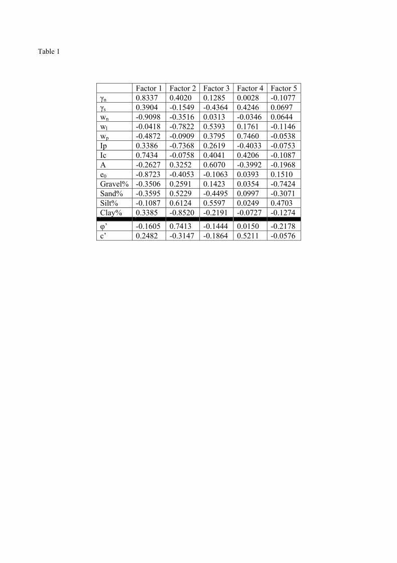
Table 1

Factor 1 Factor 2 Factor 3 Factor 4 Factor 5 γn 0.8337 0.4020 0.1285 0.0028 -0.1077 γs 0.3904 -0.1549 -0.4364 0.4246 0.0697 wn -0.9098 -0.3516 0.0313 -0.0346 0.0644 wl -0.0418 -0.7822 0.5393 0.1761 -0.1146 wp -0.4872 -0.0909 0.3795 0.7460 -0.0538 Ip 0.3386 -0.7368 0.2619 -0.4033 -0.0753 Ic 0.7434 -0.0758 0.4041 0.4206 -0.1087 A -0.2627 0.3252 0.6070 -0.3992 -0.1968 e0 -0.8723 -0.4053 -0.1063 0.0393 0.1510 Gravel% -0.3506 0.2591 0.1423 0.0354 -0.7424 Sand% -0.3595 0.5229 -0.4495 0.0997 -0.3071 Silt% -0.1087 0.6124 0.5597 0.0249 0.4703 Clay% 0.3385 -0.8520 -0.2191 -0.0727 -0.1274

φ’ -0.1605 0.7413 -0.1444 0.0150 -0.2178 c’ 0.2482 -0.3147 -0.1864 0.5211 -0.0576

Table 2

Cross-validation of 51 samples Estimator Var (Z* - Z) Corr (Z* , Z) Linear regr. coeff.

Z* = aZ + b Kriging 13.47 0.55 0.38 Multiple linear regression 12.89 0.63 0.59 Cokriging 6.76 0.81 0.79

Table 3

Cross-validation of 295 samples Estimator Var (Z* - Z) Corr (Z* , Z) Linear regr. coeff.

Z* = aZ + b Kriging 23.33 0.67 0.52 Multiple linear regression 17.72 0.76 0.58 Cokriging 14.29 0.81 0.71

Figure 1

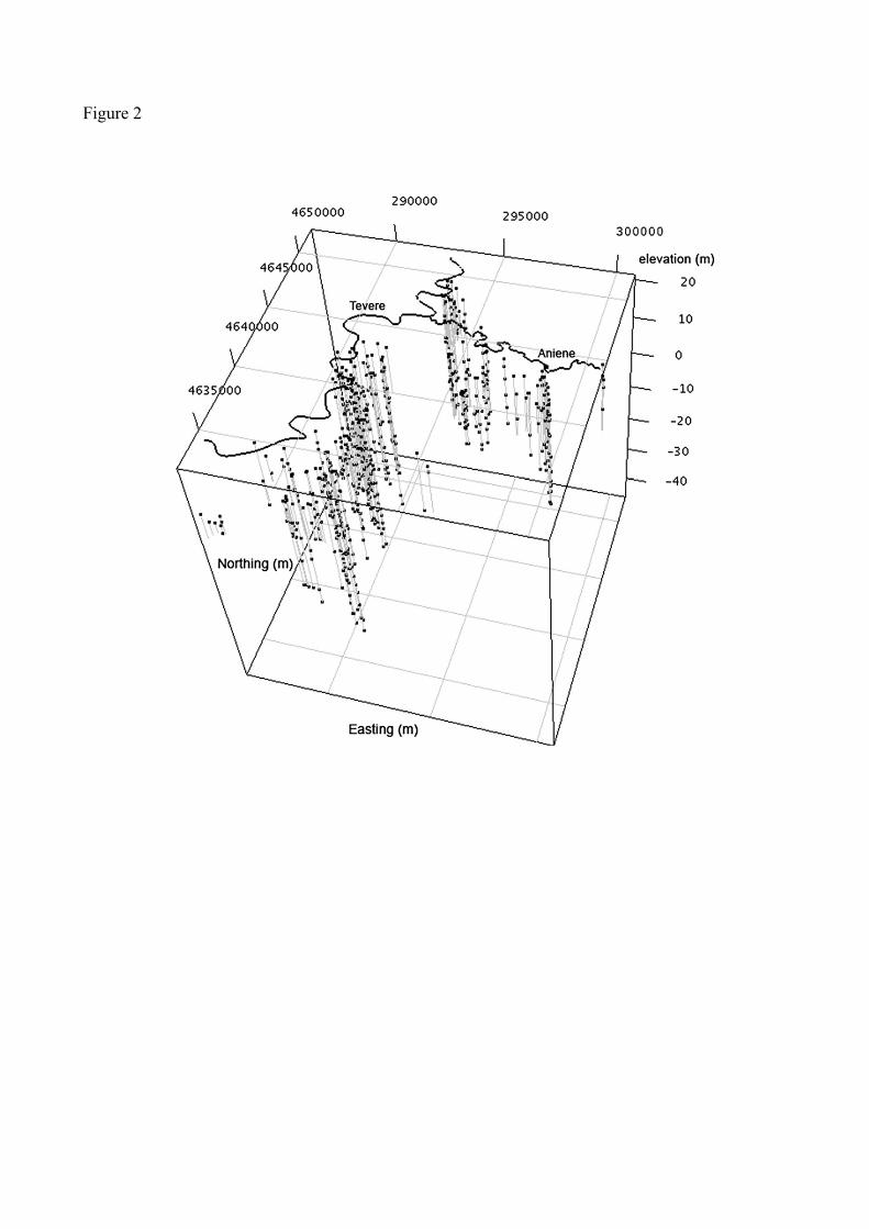
Figure 2

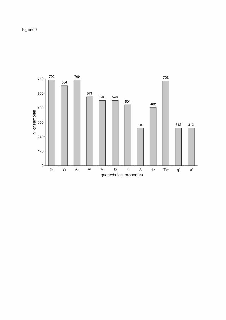
Figure 3

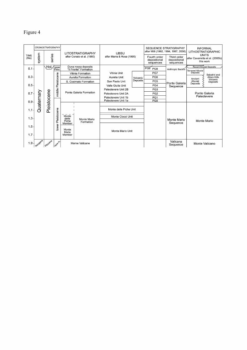
Figure 4

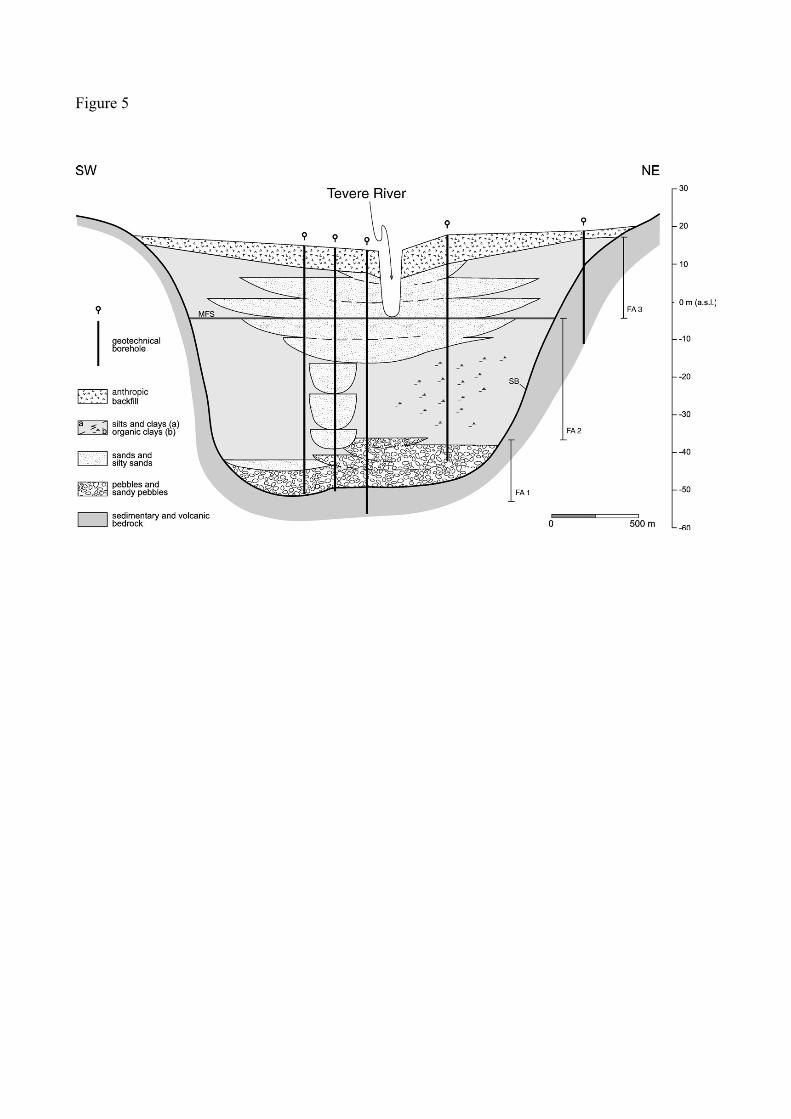
Figure 5

Figure 6

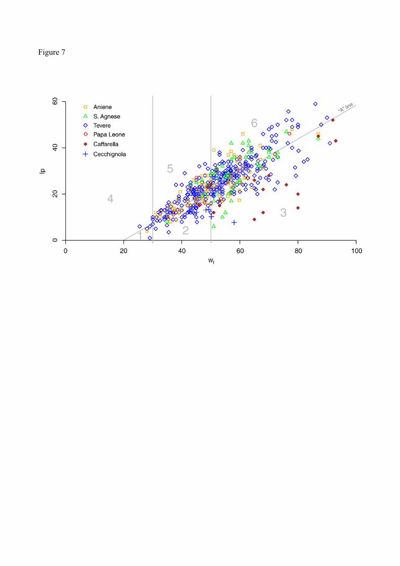
Figure 7

Figure 8

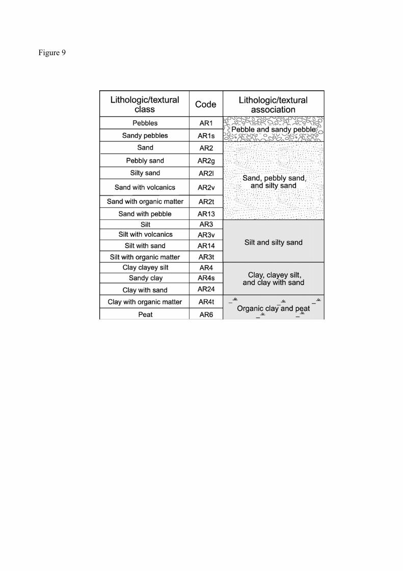
Figure 9

Figure 10a

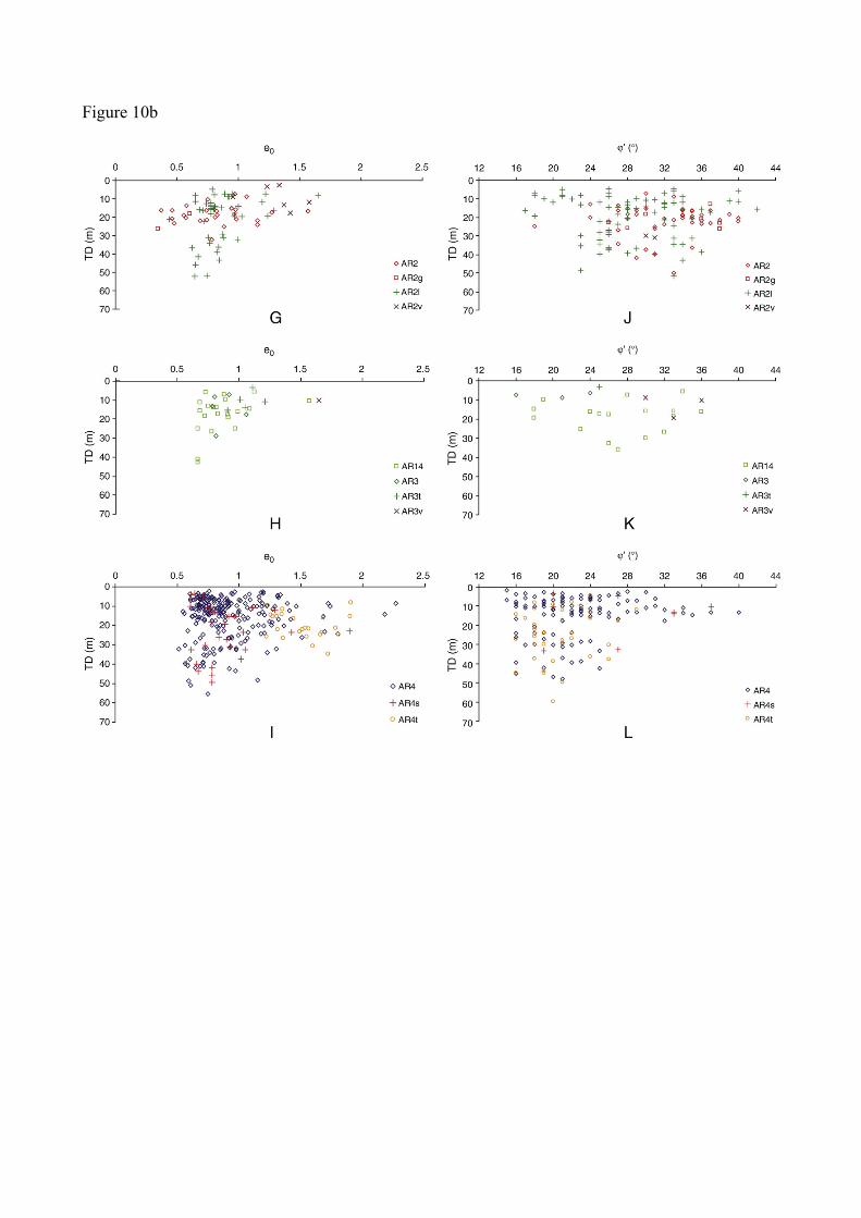
Figure 10b

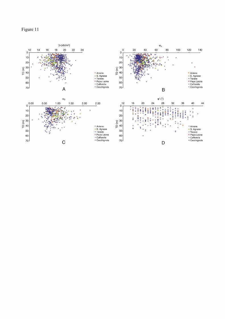
Figure 11

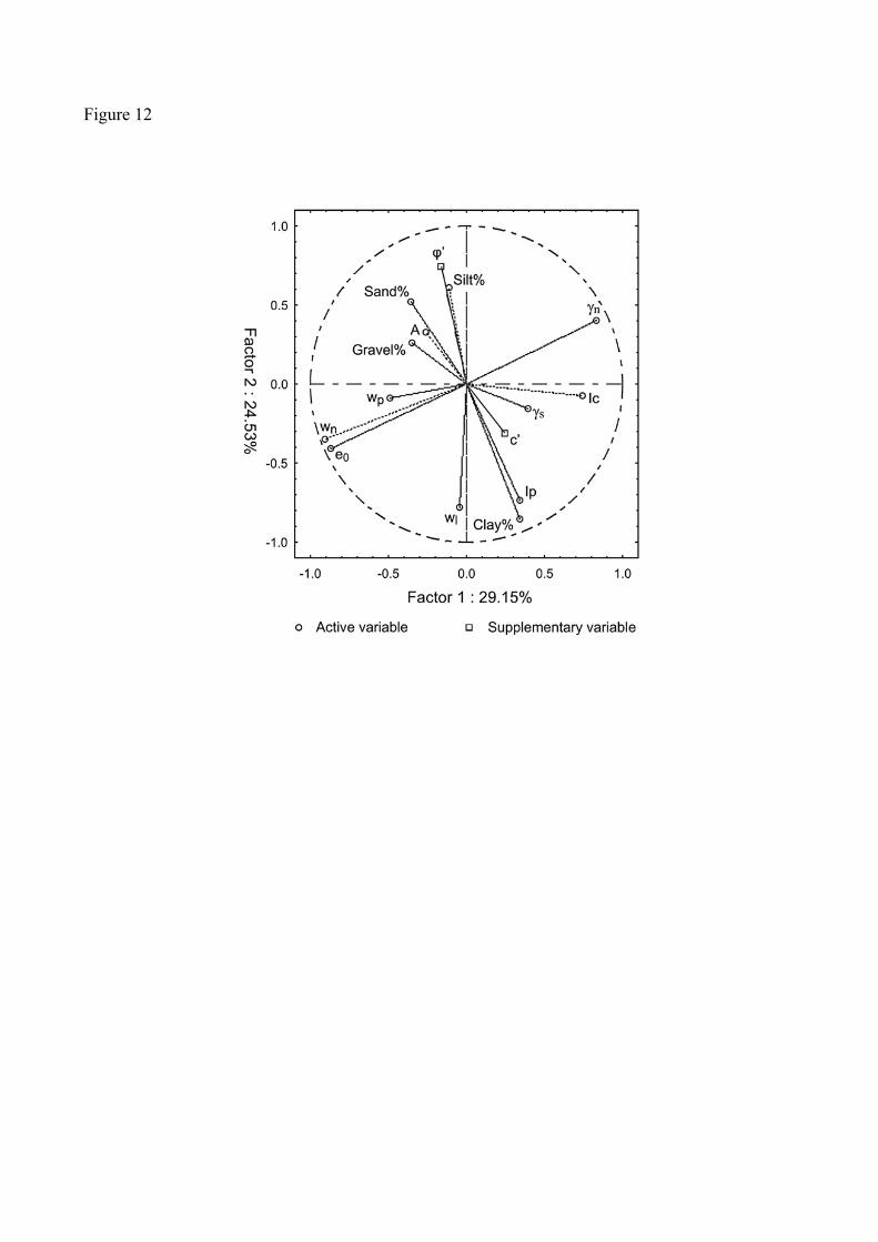
Figure 12

Figure 13

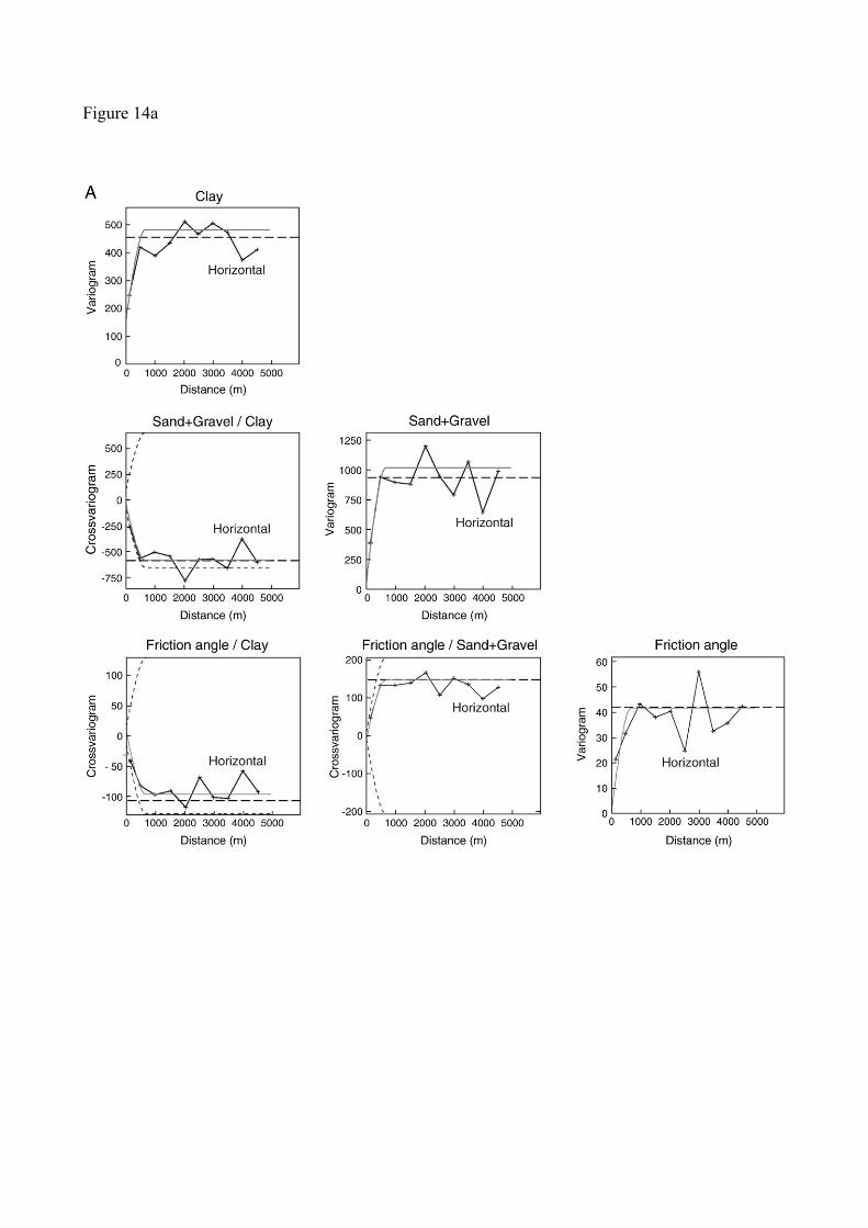
Figure 14a

Figure 14b

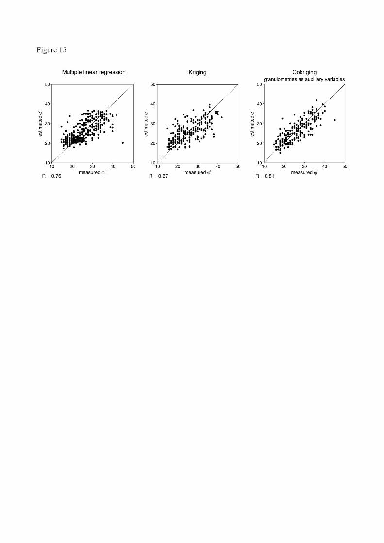
Figure 15