Spring 2017 – UAF Class GEOS 657

GEOS 657 – MICROWAVE REMOTE SENSINGSPRING 2017

Lecturer: F.J. Meyer, Geophysical Institute, University of Alaska Fairbanks; fjmeyer@alaska.edu

Lecture 13: Phase Unwrapping & Limitations of Traditional InSAR Techniques

Franz J Meyer, UAF

GEOS 657, Spring 2016 - 2

TYPICAL INSAR PROCESSING WORKFLOW

Franz J Meyer, UAF

GEOS 657, Spring 2016 - 3

A Typical InSAR Processing Workflow

1. Select and order InSAR-capable SAR data from a data server

2. Import SAR data into an InSAR processing system

3. Calculate spatial baseline & apply spectral (wavenumber) shift filtering (see Slide 50)

4. Determine co-registration parameters:

– cross-correlate >100 image chips spread over image

– use over-sampling and interpolation to locate correlation peaks

– apply regression to parameterize co-registration (e.g. affine transform)

5. Co-register images:

– Resample slave image(s) to match master image

– Required accuracy: << 1/10 resolution element

– More on required co-registration accuracy on Slides 5 & 6

Franz J Meyer, UAF

GEOS 657, Spring 2016 - 4

A Typical InSAR Processing Workflow

6. [Optional Orbit improvement: If precise orbit information is available.]

7. Interferogram formation: 𝐼 = 𝑢1 ∙ 𝑢2∗ ; optional multi-looking may be applied.

8. Flat Earth phase removal: Simulate and subtract phase trend due to the geometry changes from near range to far range.

9. Coherence Calculation: Coherence is calculated as described in Lecture 12.

10. For differential InSAR (d-InSAR): Using a DEM, simulate and subtract interferogram replicating topography-related phase.

11. Apply phase filter: A phase filter is applied to reduce InSAR phase noise and reduce phase unwrapping complexity (see next section).

12. Phase Unwrapping: Turns originally ambiguous interferometric phase into unambiguous absolute phase.

13. Geocoding and Terrain Correction: Note that flat earth phase needs to be added before geocoding to obtain absolute phase.

Franz J Meyer, UAF

GEOS 657, Spring 2016 - 5

Stripmap rule-of-thumb: 1/10 of a resolution element mis-registration is usually acceptable

Effects of Coregistration Errors on Coherence

• How accurately must the two SAR images be co-registered beforeinterferogram formation?

mis-registration in range

mis-registration in azimuth

ground resolution elementof pixel in SAR image #1 ki, ground resolution element

of pixel in SAR image #2 ki,

overlapping area: ”signal”

non-overlapping area: ”noise” (decorrelation)

Franz J Meyer, UAF

GEOS 657, Spring 2016 - 6

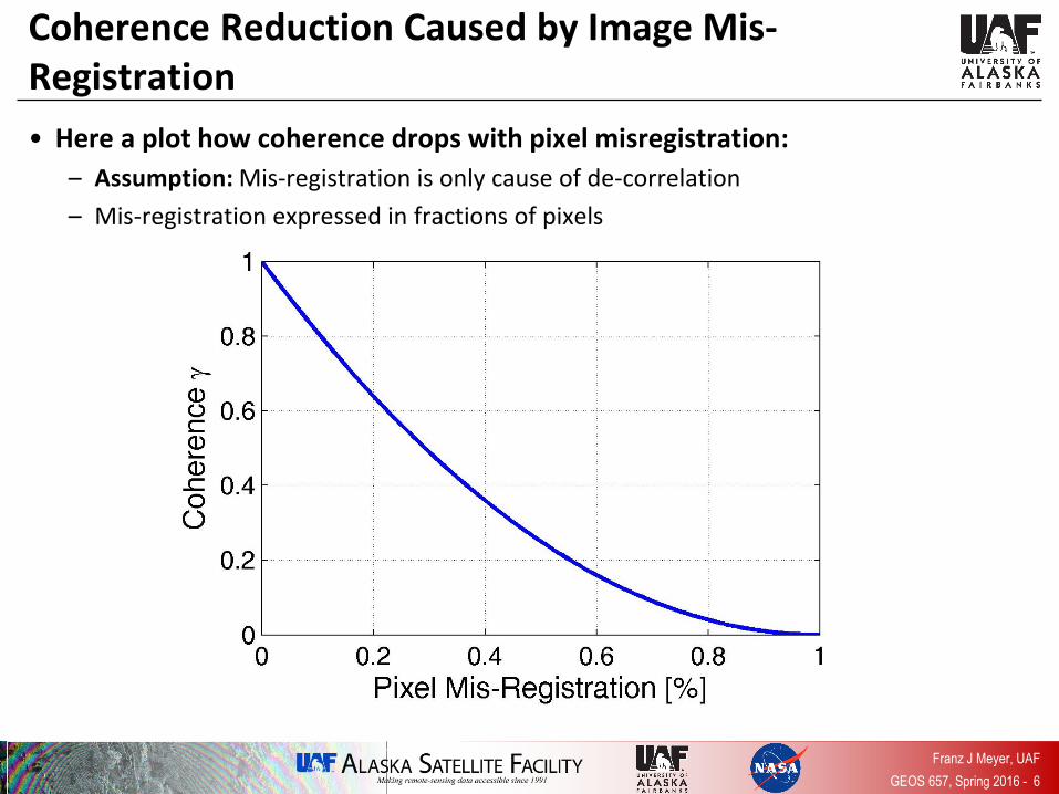
Coherence Reduction Caused by Image Mis-Registration

• Here a plot how coherence drops with pixel misregistration:

– Assumption: Mis-registration is only cause of de-correlation

– Mis-registration expressed in fractions of pixels

Franz J Meyer, UAF

GEOS 657, Spring 2016 - 7

Tips for Selecting Suitable Images for InSAR

• Required conditions:

– Images from identical orbit direction (both ascending or both descending)

– Images with identical incidence angle and beam mode

– Images with identical resolution and wavelength (usually: same sensor)

– Images with same viewing geometry (same track/frame combination)

• Recommended conditions:

– For topographic mapping: Limited time separation between images (temporal baseline)

– For deformation mapping: Limited spatial separation of acquisition locations (spatial baseline)

– Images from similar seasons / growth / weather conditions

How to select a suitable image pair for successful InSAR processing

Franz J Meyer, UAF

GEOS 657, Spring 2016 - 8

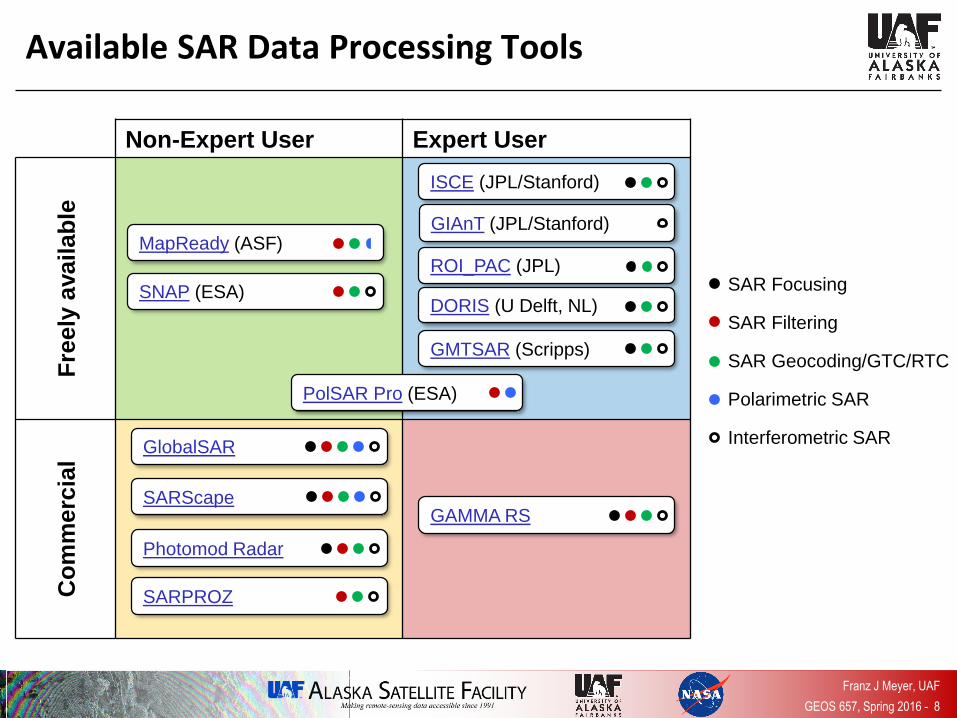
Available SAR Data Processing Tools

Non-Expert User Expert User

Fre

ely

availab

leC

om

merc

ial

SAR Focusing

SAR Filtering

SAR Geocoding/GTC/RTC

Polarimetric SAR

Interferometric SAR

ROI_PAC (JPL)

ISCE (JPL/Stanford)

DORIS (U Delft, NL)

GMTSAR (Scripps)

MapReady (ASF)

SNAP (ESA)

PolSAR Pro (ESA)

GlobalSAR

SARScape

Photomod Radar

GAMMA RS

GIAnT (JPL/Stanford)

SARPROZ

Franz J Meyer, UAF

GEOS 657, Spring 2016 - 9

Non-Expert Free Software Packages

• MapReady (https://www.asf.alaska.edu/data-tools/mapready/)– Available from:

– Sensors

• ERS-1 (ASF & ESA format), ERS-2 (ASF & ESA format), Radarsat-1 (ASF format), ALOS PALSAR

– Capabilities

• Conversion of SAR data to Geotiff and JPG format

• Data Visualization

• Geocoding

• Terrain Correction (Geometric and Radiometric)

• Some Polarimetric tools

Franz J Meyer, UAF

GEOS 657, Spring 2016 - 10

Non-Expert Free Software Packages

• Sentinel Applications Platform (SNAP; http://step.esa.int/main/download/)– Available from: European Space Agency (ESA)

– Sensors

• ERS-1, ERS-2, ENVISAT ASAR (all ESA format), Radarsat-1, Radarsat-2 (MDA format), ALOS PALSAR, Sentinel-1

– Capabilities

• Conversion of SAR data to Geotiff and JPG format and kmz format

• Data Visualization

• Geocoding (not for PALSAR)

• Terrain Correction (Geometric and Radiometric) (not for PALSAR)

• InSAR processing

• Some Polarimetric tools

Franz J Meyer, UAF

GEOS 657, Spring 2016 - 11

Get DEM Data

• For RTC and GTC, DEM information is required

• NEST is automatically downloading DEM data during processing

• For MapReady, DEM data needs to be provided by the user

• Free Access to DEM data is available through EarthExplorer(http://earthexplorer.usgs.gov/)

Franz J Meyer, UAF

GEOS 657, Spring 2016 - 12

THE CONCEPTS OF PHASE UNWRAPPING

Franz J Meyer, UAF

GEOS 657, Spring 2016 - 13

Think – Pair – Share

Formulating the problem of phase unwrapping:

• Q1: In the figure below, try to draw the unwrapped phase 𝜙 based on the observed wrapped phase 𝜓 = 𝑊 𝜙 .

What do you think the true unwrapped phase looks like and what rule did you (implicitly) apply to come up with your conclusion?

Franz J Meyer, UAF

GEOS 657, Spring 2016 - 14

Interferometric Phase is Ambiguous

good fringe quality13/14 Jan. 1996

bad fringe quality23/24 March 1996

data ERS-1/2 © ESA

Franz J Meyer, UAF

GEOS 657, Spring 2016 - 15

kiF

kiFkiF

k

i

,

,,

2-D scalar field: kiF ,

kiFkiFkiF

kiFkiFkiF

k

i

,1,,

,,1,

partial

derivatives:

gradient:

i 1i

1k

kFi

Fk F

1k

1i

Derivatives of 2-D Functions on a Regular Discrete Grid: Gradient

Franz J Meyer, UAF

GEOS 657, Spring 2016 - 16

or [phase cycles]

Phase Unwrapping Problem Statement

interferometric phase: kikiki NT ,,,

useful (e.g. topography induced) phase phase noise

wrapped phase: kiWki ,,

with W : wrapping operator

and [rad]

“absolute” phase

ki,Given find an estimate or even .

ki,

kiT ,phase unwrapping problem:

many solutions possible additional constraints required (smoothness, ...)

find „most likely“ phase

ki,

2

1

2

1

Franz J Meyer, UAF

GEOS 657, Spring 2016 - 17

Find the “Most Likely” Solution

... than this this is much more likely ...

Mt. Etna, data ERS-1/2 © ESA

Franz J Meyer, UAF

GEOS 657, Spring 2016 - 18

kiA

kiAkiA

k

i

,

,,

2-D vector field:

curl:

i 1i

1k

k

4

,

,1,,,1

,,,

C

iikk

ikki

cdkiA

kiAkiAkiAkiA

kiAkiAkiA

4C

Derivatives of 2-D Functions on a Regular Discrete Grid: Curl

note: curl of a 2-D vector field is a scalar

vector product

Franz J Meyer, UAF

GEOS 657, Spring 2016 - 19

- 0.5

0.5

- 0.5

0.5

Unwrapping of a 1-D Phase Ramp: High Coherence

samplecyclesslope 2.0 9.0

Franz J Meyer, UAF

GEOS 657, Spring 2016 - 20

- 0.5

0.5

- 0.5

0.5

!

Unwrapping of a 1-D Phase Ramp: Medium Coherence

75.0

- 0.5

0.5

unwrapping error: 1 cycle lost

Franz J Meyer, UAF

GEOS 657, Spring 2016 - 21

If and

2-D Phase Unwrapping Methods:Gradient-Based Phase Unwrapping

kikikik ,,ˆ, kii ,

kiW

kiWki

k

i

,

,,ˆ

simple gradient estimate: „wrapped gradient of wrapped phases“

ki,1. Find an estimate of based on : ki, ki,ˆ

2. Integrate to get ki,ˆ ki,

in reality:

i.e. is in general not conservative and the integration result depends on the path

(note: per definition)

0,ˆ,,ˆ kikiki

ki,ˆ

0, ki

Franz J Meyer, UAF

GEOS 657, Spring 2016 - 22

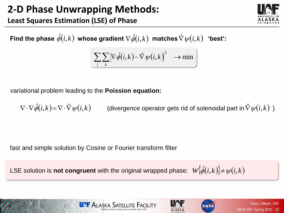
2-D Phase Unwrapping Methods: Least Squares Estimation (LSE) of Phase

Find the phase whose gradient matches ‘best‘: ki,ˆ ki, ki,

min,ˆ,ˆ2

i k

kiki

variational problem leading to the Poission equation:

kiki ,ˆ,ˆ (divergence operator gets rid of solenoidal part in ) ki,ˆ

fast and simple solution by Cosine or Fourier transform filter

LSE solution is not congruent with the original wrapped phase: kikiW ,,ˆ

Franz J Meyer, UAF

GEOS 657, Spring 2016 - 23

2-D Phase Unwrapping Methods: Slope Bias in LSE Phase Unwrapping

LSE systematically underestimates slopes (slope bias)

Options for reducing slope bias:

• weighted LSE:

• use more sophisticated gradient estimates: local fringe frequency estimators

min,ˆ,ˆ,2

i k

kikikic

kic , : weighting function, high where gradient estimate is assumed to be reliable (and conservative) and vice versa

Original wrapped

phase

Rewrappedunwrappedphase

ki, kiW ,

Franz J Meyer, UAF

GEOS 657, Spring 2016 - 24

2-D Phase Unwrapping Methods: The “Residue” Approach

4

)cycle(1:or2

)cycle(1:or2

0

,ˆ,ˆ,resC

kicdkiki

i 1i

1k

k

4C

For a conservative field any closed integration path must give zero integral value!

test field for conservativeness by

computing the smallest closed integrals C4

for every quadrupel of pixels

residue field

ki,ˆ

no residue

positive residue

negative residue

A Word on Residues:

Franz J Meyer, UAF

GEOS 657, Spring 2016 - 25

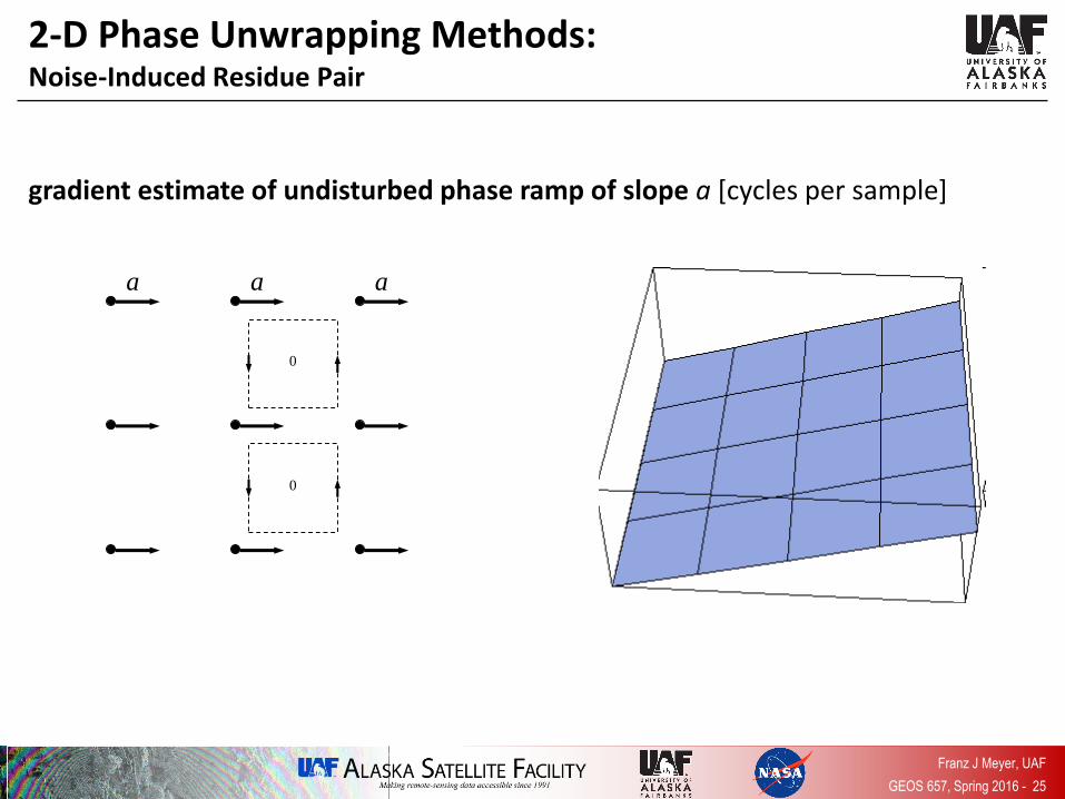
2-D Phase Unwrapping Methods: Noise-Induced Residue Pair

0

0

gradient estimate of undisturbed phase ramp of slope a [cycles per sample]

a a a

Franz J Meyer, UAF

GEOS 657, Spring 2016 - 26

2-D Phase Unwrapping Methods: Noise-Induced Residue Pair

gradient estimate of phase ramp disturbed by noise 𝜺

0

0

a a a

a

a

Franz J Meyer, UAF

GEOS 657, Spring 2016 - 27

2-D Phase Unwrapping Methods: Noise-Induced Residue Pair

gradient estimate of phase ramp disturbed by noise 𝜺 causing aliasing

1

1

a a a

1a

a

erroneous gradient estimates residue dipoles

Franz J Meyer, UAF

GEOS 657, Spring 2016 - 28

2-D Phase Unwrapping Methods: Topography-Induced Residue Pair

ki,absolute phase: ki,wrapped phase:

positive residuenegative residue

> 1 cycle

Franz J Meyer, UAF

GEOS 657, Spring 2016 - 29

2-D Phase Unwrapping Methods: Branch Cut Methods

• group positive and negative residues to dipoles and connect them by branch-cuts (or: cut lines)

• use branch cuts ...

– either: to direct integration path for phase unwrapping such that no branch-cut is crossed

– or: to modify gradient estimate by adding a full cycle along the branch-cut:

cycle1

kidkiki ,,ˆ,ˆ

kid ,

kikid ,res,

where

kikiW ,,ˆ

Franz J Meyer, UAF

GEOS 657, Spring 2016 - 30

2-D Phase Unwrapping Methods:Typical Residue Distribution

red: positive residuegreen: negative residueblue: branch cut

Franz J Meyer, UAF

GEOS 657, Spring 2016 - 31

2-D Phase Unwrapping Methods: Branch Cut Methods – The Minimum Cost Flow Algorithm (I)

nodes

arcs (with costs)

outflow = –1 inflow = +1

+

+–

–

Franz J Meyer, UAF

GEOS 657, Spring 2016 - 32

2-D Phase Unwrapping Methods: Branch Cut Methods – The Minimum Cost Flow Algorithm (II)

• Graph theory and network programming gives fast solution for

• Result: , a vector field whose elements are integers [cycles] (mostly: 0, -1, 1)

• is used for correcting and making gradient estimate conservative:

• Phase unwrapping find optimum cost function

min,,,, i k

kk

i k

ii kidkickidkic

kid ,

minimum cost flow

kid ,

kidkiki ,,ˆ,ˆ

kic ,

Franz J Meyer, UAF

GEOS 657, Spring 2016 - 33

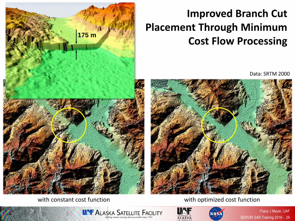
2-D Phase Unwrapping Methods: Cost Function and Branch Cuts

., constkic ...gradient,phase,, fkic

Franz J Meyer, UAF

SERVIR SAR Training 2016 - 29

with optimized cost function

175 m

with constant cost function

Data: SRTM 2000

Improved Branch Cut Placement Through Minimum

Cost Flow Processing

Franz J Meyer, UAF

GEOS 657, Spring 2016 - 35

LIMITATIONS OF CONVENTIONAL INSAR

Franz J Meyer, UAF

GEOS 657, Spring 2016 - 36

Error Sources from:• Variation of

atmospheric signal

delays 𝜙𝑎𝑡𝑚𝑜

• Uncertainties of the

orbit geometry 𝜙𝑜𝑟𝑏𝑖𝑡

• Noise from signal

decorrelation 𝜙𝑛𝑜𝑖𝑠𝑒

Recap of InSAR Acquisition Scenario

z

1tt

R

4defo defoR

defo

defoR

1tt

2tt

terrain motion

or subsidence

Interferometric Phase:

atmo orbit noise

B2tt

Bztopo ;

R

RRR

Franz J Meyer, UAF

GEOS 657, Spring 2016 - 37

The Complete InSAR Phase Equation

• Phase of an interferogram:

𝜙 = 𝑊 𝜙𝑡𝑜𝑝𝑜 + 𝜙𝑑𝑒𝑓𝑜 + 𝜙𝑎𝑡𝑚𝑜 + 𝜙𝑜𝑟𝑏𝑖𝑡 + 𝜙𝑛𝑜𝑖𝑠𝑒

= 𝑊4𝜋

𝜆

𝐵⊥𝑅 ⋅ 𝑠𝑖𝑛 𝜃

ℎ +4𝜋

𝜆𝑣 ∙ ∆𝑡 + 𝜙𝑎𝑡𝑚𝑜 + 𝜙𝑜𝑟𝑏𝑖𝑡 + 𝜙𝑛𝑜𝑖𝑠𝑒

(𝑊: wrapping operator → 𝜙: −𝜋, 𝜋 )

• Phase of a differential interferogram (after compensation of topography phase):

Δ𝜙 = 𝑊4𝜋

𝜆

𝐵⊥𝑅 ⋅ 𝑠𝑖𝑛 𝜃

ℎ𝑒𝑟𝑟 +4𝜋

𝜆𝑣 ∙ ∆𝑡 + 𝜙𝑎𝑡𝑚𝑜 + 𝜙𝑜𝑟𝑏𝑖𝑡 + 𝜙𝑛𝑜𝑖𝑠𝑒

(where ℎ𝑒𝑟𝑟 = ℎ𝑡𝑟𝑢𝑒 − ℎ𝐷𝐸𝑀 is a residual topography phase due to errors in the DEM)

Franz J Meyer, UAF

GEOS 657, Spring 2016 - 38

Limitations and Error Sources of InSAROverview

1. Only sensitive to motion in sensor’s line-of-sight → does not provide 3D motion fields

2. Temporal baseline is limited, leading to limited sensitivity to very slow surface motion:

– Limitation is due to temporal decorrelation, leading to increase of phase noise with time

3. Spatial baseline is limited, limiting number of interferograms that can be formed from a stack of SAR data

4. Atmospheric phase patterns may mask signal of interest, limiting sensitivity of InSAR to very small motion (or topography) signals

5. Orbit errors may cause ramp-like phase distortions (usually small)

Franz J Meyer, UAF

GEOS 657, Spring 2016 - 39

Limitations of InSAR:1. Only Line-of-Sight Motion Sensitivity

SAR

V

y

x

R

z

z

R

cossin zyR

for ERS:

1 fringe ( ) corresponds to

2.8 cm in R

3.0 cm in z (e.g. subsidence)

7.2 cm in y (motion)

2

y! only 1 dimension of 3-d motion accessible

! no sensitivity to motion in x direction

Franz J Meyer, UAF

GEOS 657, Spring 2016 - 4040

Limitations of InSAR:2. Temporal Signal Decorrelation

• Changes of the ground scattering properties are main source of signal decorrelation with time

– Example: Airborne C-band SAR over vegetated environments

short term interferogram (15.01 – 21.01)

long term interferogram (15.01 – 20.02)

Franz J Meyer, UAF

GEOS 657, Spring 2016 - 41

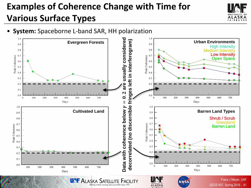
Examples of Coherence Change with Time for Various Surface Types• System: Spaceborne L-band SAR, HH polarization

Evergreen Forests Urban EnvironmentsHigh Intensity

Medium IntensityLow IntensityOpen Space

Cultivated Land Barren Land Types

Shrub / ScrubGrassland

Barren LandD

ata

wit

h c

oh

ere

nc

e b

elo

w 𝜸=𝟎.𝟐

are

us

ua

lly c

on

sid

ere

d

de

co

rre

late

d(n

o d

isc

ern

ible

fri

ng

es

le

ft in

in

terf

ero

gra

m)

Franz J Meyer, UAF

GEOS 657, Spring 2016 - 42

Examples of Coherence Change with Time Boreal Dry Climate

• Example: Delta Junction – L-band SAR (ALOS PALSAR)

Franz J Meyer, UAF

GEOS 657, Spring 2016 - 43

Examples of Coherence Change with Time Boreal Dry Climate

• Delta Junction – Example for Subset-1

• LULC: Woody Savannas

• Flat region

• Summer (June to Oct), Winter

(Nov. to May)

Franz J Meyer, UAF

GEOS 657, Spring 2016 - 44

Examples of Coherence Change with Time Boreal Dry Climate

• Estimated Coherence Models – Delta Junction; L-band

– Coherence Model Characteristics:

ҧ𝛾 𝑡 = 𝑨 ∙ 𝒄𝒐𝒔 𝟐𝝅𝝀 ∙ 𝒕 + 𝝓 + 𝑩 ∙ 𝒆𝒙𝒑 −𝒅 ∙ 𝒕

Ob

servation

sM

od

el Resu

lts

• Different exponential decay parameters (𝑑 & 𝐵)

• Significant & similar periodic cycle 𝝀 for analyzed land covers

• Differences in amplitude 𝐴 of periodic signal

• Periodicity 𝜆 closely one year near-seasonal signatures

• Good model fit (high 𝑅2)

LULC type A λ (1/yr) ϕ B d (1/yr) 𝑹𝟐

1. Woody Savannas 0.08± 0.01

0.99± 0.01

0.00± 0.17

0.31± 0.01

0.18± 0.02

0.89

2. Open Shrublands 0.06± 0.01

0.99± 0.02

0.03± 0.23

0.44± 0.01

0.23± 0.02

0.92

3. Urban & Croplands 0.03± 0.01

1.01± 0.03

0.00± 0.47

0.25± 0.01

0.26± 0.03

0.80

4.Evergreen Forest 0.05± 0.01

0.99± 0.03

0.00± 0.43

0.39± 0.02

0.21± 0.03

0.76

Franz J Meyer, UAF

GEOS 657, Spring 2016 - 45

Limitations of InSAR:2. Temporal Signal Decorrelation

Example: Volcano Monitoring

• Often, caldera of active volcanoes is decorrelated due to constant change (snow and ice melt; ash fall; lahars; lava flows; …).

• Consequence:

– Area with strongest signals inaccessible

– In modeling, shape of source model as well as horizontal location of source hard to define

– combination with GPS is advised

Caldera of Westdahl Peak is

decorrelated in all interferograms

Franz J Meyer, UAF

GEOS 657, Spring 2016 - 46

Limitations of InSAR:3. Limited Spatial Baselines

• Long spatial baselines lead to decorrelationof interferograms

• Figure: Fringe density increases with baseline length!

• At certain baseline length (critical baseline 𝑩⊥,𝒄𝒓𝒊𝒕) the fringes become closer than the pixel size:

phase jump from pixel to pixel > 2𝜋

phase image becomes random

Sh

ort B

aselin

e

Inte

rfero

gra

m

Lo

ng

Baselin

e

Inte

rfero

gra

m

Franz J Meyer, UAF

GEOS 657, Spring 2016 - 47

Limitations of InSAR:How to Calculate the Critical Baseline 𝐵⊥,𝑐𝑟𝑖𝑡

• We can calculate the fringe frequency in the interferogram from:

∆𝑓 𝛼 = −𝑐 ∙ 𝐵⊥

𝑅 ∙ 𝜆 ∙ 𝑡𝑎𝑛 𝜃 − 𝛼

1

𝑠𝛼: terrain slope

• Critical baseline if we have one fringe of phase change per pixel, corresponding

to 𝟐∆𝒇 𝜶

𝒄=

𝟏

𝝆𝒓(with range resolution 𝝆𝒓):

1

𝜌𝑟= −

2 ∙ 𝐵⊥,𝑐𝑟𝑖𝑡𝑅 ∙ 𝜆 ∙ 𝑡𝑎𝑛 𝜃 − 𝛼

⟹ 𝐵⊥,𝑐𝑟𝑖𝑡 =𝑅 ∙ 𝜆 ∙ 𝑡𝑎𝑛 𝜃 − 𝛼

2 ∙ 𝜌𝑟𝑚

• Dependencies:

– Higher range resolution (smaller 𝜌𝑟) → 𝐵⊥,𝑐𝑟𝑖𝑡 increases

– Steeper slopes (larger 𝛼) → 𝐵⊥,𝑐𝑟𝑖𝑡 decreases

– Longer wavelength 𝜆 → 𝐵⊥,𝑐𝑟𝑖𝑡 increases

Franz J Meyer, UAF

GEOS 657, Spring 2016 - 48

Critical Baseline 𝐵⊥,𝑐𝑟𝑖𝑡 for Various Sensors

• Assumptions:

– Surface slope 𝛼 = 0°

– Incidence angle θ = 25°

– Range to ground 𝑅 ≈ 800,000𝑚

• 𝑩⊥,𝒄𝒓𝒊𝒕 for various sensor systems @ 𝜽 = 𝟐𝟓° :

– ERS-1/2 & Envisat Stripmap mode: 𝐵⊥,𝑐𝑟𝑖𝑡 ≈ 1,100𝑚

– ALOS PALSAR:

• FBS mode: 𝐵⊥,𝑐𝑟𝑖𝑡 ≈ 8,500𝑚

• FBD & PLR mode: 𝐵⊥,𝑐𝑟𝑖𝑡 ≈ 4,250𝑚

– TerraSAR-X Stripmap mode: 𝐵⊥,𝑐𝑟𝑖𝑡 ≈ 5,800𝑚

Franz J Meyer, UAF

GEOS 657, Spring 2016 - 49

Limitations of InSAR:Critical Baseline 𝐵⊥,𝑐𝑟𝑖𝑡 - A Frequency-Space Explanation (I)

SAR #1 SAR #2

0ff

sin20

yfcff

1 2

y

yf1

f

• An oblique SAR acquisition transforms object spectrum into observed signal spectrum:

Franz J Meyer, UAF

GEOS 657, Spring 2016 - 50

Limitations of InSAR:Critical Baseline 𝐵⊥,𝑐𝑟𝑖𝑡 - A Frequency-Space Explanation (II)

• An oblique SAR acquisition transforms ground range reflectivity (object) spectrum into observed signal spectrum:

0ff

yf

0fW

Spectral shift filtering: cut off non-overlapping spectral bands

Franz J Meyer, UAF

GEOS 657, Spring 2016 - 51

Identical to Equation on Slide 43

Limitations of InSAR:Critical Baseline 𝐵⊥,𝑐𝑟𝑖𝑡 - A Frequency-Space Explanation (III)

fW

cy

2interferometric range resolution:

See Top of Slide 43

tan

,

R

Bcf

effectivespectral shift = fringe frequency: : terrain slope

c

RWB crit

tan,

𝑊: range signal bandwidth (e.g. 15.5 MHz for ERS)

critical (= maximum) baseline ( ): Wf

Franz J Meyer, UAF

GEOS 657, Spring 2016 - 52

Limitations of InSAR:Critical Baseline 𝐵⊥,𝑐𝑟𝑖𝑡 - A Frequency-Space Explanation (III)

-75 -50 -25 0 25 50 75

tfihs l

artce

psdeg23

degterrain slope

deg90

shadowlay-over

blindangles

MHz5.15

MHz5.15

mB 200

Franz J Meyer, UAF

GEOS 657, Spring 2016 - 53

Limitations of InSAR: 4. Atmospheric Distortions

53

• Atmospheric propagation influence:

– Masks deformation signals in InSAR

– Increases data requirements and latency times for InSAR analyses

What we often get

What we would like

~ -3 cm/y subsidence

Franz J Meyer, UAF

GEOS 657, Spring 2016 - 54

Examples of Atmospheric Phase Distortions in InSAR Data

• 8 100x100 km interferograms showing atmospheric distortions [cm]

Courtesy: R. Hansen, TU Delft

Franz J Meyer, UAF

GEOS 657, Spring 2016 - 55

Limitations of InSAR: 4. Atmospheric Distortions

Atmospheric Signals can lead to incorrect interpretation of observations:

mm

d-InSAR Observations,

Big Island, Hawaii

Is the volcano inflating?

Upcoming eruption?

Atmospheric Model d-InSAR – Atmospheric Model

Mauna Kea

Mauna Loa

Franz J Meyer, UAF

GEOS 657, Spring 2016 - 56

What’s Next?

• This is what awaits next week:

– Tuesday: 5-minute short term project concept presentations

– Thursday : Lab on InSAR Processing Using the SNAP Toolbox

Mid-term …