geophysical techniques used in volcanogenic massive
TRANSCRIPT

GEOPHYSICAL TECHNIQUES USED IN VOLCANOGENIC
MASSIVE SULPHIDES EXPLORATION IN THE ARCHEAN
GREENSTONE BELT OF WESTERN KENYA
CASE STUDY YALA-(KAKAMEGA)
SGL 413: PROJECT IN GEOLOGY
MBAU GITONGA
REGISTRATION NO. I13/2354/2007
A dissertation submitted to the department of Geology of the University of Nairobi as
partial fulfillment for the degree of Bachelor of Science in Geology
JUNE 2011

ii
DECLARATION AND APPROVAL
Declaration by Candidate
I declare that this is my original work and has not been presented for examination elsewhere.
Name: Mbau Gitonga (I13/2354/2007)
Signature……………………………………………………………….
Date………………………………………………………………………
Approval by Advisor
Prof. J. O Barongo
Department of Geology
Signature…………………………………………………………………..
Date………………………………………………………………………..
Approval by Supervisors
Name………………………………………………………………………
Department of Geology
Signature…………………………………………………………………..
Date………………………………………………………………………..

iii
ABSTRACT A prospect is restricted volume of ground that is considered to have the possibility of directly
hosting an ore body. As earth scientist therefore we look for ways of imaging the subsurface to
rule out the question of a prospect. This project addresses how to use electromagnetic technique
in imaging or locating conductive volcanogenic massive sulphides (VMS) and how geology
influences mineralization. The case study area Yala- Kakamega located in Busia County with
coordinates 0.06° and 34.32° where a ground follow up of an input airborne electromagnetic
survey was conducted (Barongo 1987). Observations from the interpreted data in this report
showed that graphite and Pyrite bodies which constitute the main target ore bodies reach near
ground surface. The ore body also occurs mostly in the andesites and rhyolites rocks
(Kavirondian system) as well as they are nearly vertically dipping due to the folding structures of
the area. This correlation is useful in geological mapping. The electromagnetic method therefore
is a simple technique which does not require any expensive trenching and is very effective in
delineating these ore bodies.

iv
ACKNOWLEGDMENT I express my deepest appreciation to my advisor Prof. J.O Barongo for the commitment he has
shown in guiding me in my work. I also thank Dr. Daniel Olago and Dr. C. Gichaba, my course
coordinators for their tremendous efforts in seeing me through this project. This work would not
have been accomplished without their help. I am greatly indebted to the Ministry of Environment
and Mineral Resources for their library materials. Finally, my dear parents, siblings and to all my
classmates for their support.
v
Table of Contents DECLARATION AND APPROVAL ...................................................................................... ii
ABSTRACT............................................................................................................................. iii
ACKNOWLEGDMENT ......................................................................................................... iv
CHAPTER 1 ..............................................................................................................................1
1.1 Introduction .....................................................................................................................1
1.2 Statement of the Problem ...................................................................................................2
1.3 Objectives ..........................................................................................................................2
1.4 Methodology .....................................................................................................................2
1.5 Justification .......................................................................................................................2
1.6 Aim ...................................................................................................................................2
1.7 GEOGRAPHY OF YALA (KAKAMEGA) .......................................................................3
1.8 Geology of Yala –Kakamega .............................................................................................4
1.8.1 Geological Setting .......................................................................................................4
1.8.2 Structural Geology ......................................................................................................5
CHAPTER 2 ..............................................................................................................................7
2.1 BASIC PRINCIPLES ..........................................................................................................7
2.1.1 Electromagnetic Methods ............................................................................................7
2.1.1.1 Frequency Domain E.M Method ...........................................................................8
2.1.1.2 Time Domain E.M System (TDEM) .....................................................................9
CHAPTER 3 ............................................................................................................................ 11
3.0 METHODOLOGY ............................................................................................................ 11
3.1 TIME DOMAIN AIRBORNE EM METHOD .............................................................. 11
3.1.1 Field Proceedures................................................................................................... 11
3.2 Ground Geophysical Surveys ....................................................................................... 13
3.2.1 Field Proceedure ................................................................................................... 13
3.2.2 HLEM ....................................................................................................................... 14
3.2.2.1 Field procedure ................................................................................................... 14
CHAPTER 4 ............................................................................................................................ 17
4.0 RESULTS and INTERPRETATION ............................................................................... 17
4.1 Results ...................................................................................................................... 17

vi
4.1.1 RECONNAISSANCE AEM RESULTS .................................................................... 17
4.1.2 Interpretation ............................................................................................................. 17
4.1.3 Detailed Ground Survey Results ................................................................................ 20
4.1.3.1 VLEM Results .................................................................................................... 20
4.1.3.2 Interpretation ...................................................................................................... 21
4.1.3.3 HLEM RESULTS ............................................................................................... 21
4.1.3.4 Interpretation ...................................................................................................... 22
CHAPTER 5 ............................................................................................................................ 25
5.0 DISCUSSION CONCLUSION AND RECOMMENDATION ........................................ 25
5.1 DISCUSSION.................................................................................................................. 25
5.2 Conclusion ....................................................................................................................... 25
5.3 Recommendation ............................................................................................................. 26
REFERENCES ........................................................................................................................ 27
APPENDIX I ........................................................................................................................... 28
DATA RESULTS FOR VLEM AND HLEM SURVEY .................................................... 28
VLEM DATA....................................................................................................................... 28
HLEM DATA FOR 125W ................................................................................................... 28
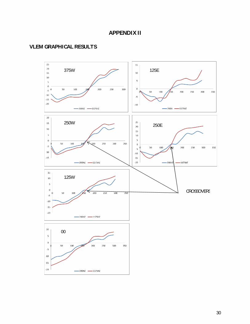
APPENDIX II .......................................................................................................................... 30
VLEM GRAPHICAL RESULTS ....................................................................................... 30
APPENDIX III ........................................................................................................................ 31
FREE-AIR PHASOR DIAGRAMS .................................................................................... 31
LIST OF FIGURES
Figure 1.1 Geographical location of the study area in a blue dot. .................................................3
Figure 1.2 Geological Cross section of the region. . .....................................................................4
Figure 1.3 Figure 1.3 Geological map of Yala – Kakamega area..................................................5
Figure 2.1 Primary and secondary fields in the horizontal loop induction method. (b) Amplitudes
and phases of the primary (p) and secondary (s) fields.). .............................................................6
Figure 2.2 Transmitter current pulse and current decay after current is switched off.. ..................8
Figure 3.1 Airbone EM Survey plan.. ........................................................................................ 10
vii
Figure 3.2 (a) Plan view of VLEM field procedure (b) strike direction of a conductor.. ............. 11
Figure 3.3 (a) Plan view of HLEM field procedure(b) Tx-Rx configuration over a conductor.. .. 13
Figure 1.1 Geographical location of the study area in a blue dot. .............................................................. 3
Figure 1.1 Geographical location of the study area in a blue dot. .............................................................. 3
Figure 1.1 Geographical location of the study area in a blue dot. .............................................................. 3 Figure4.3 Crone fixed transmitter vertical loop EM profiles across anomaly p.. ........................ 17
Figure 1.1 Geographical location of the study area in a blue dot. .............................................................. 3
Figure 1.1 Geographical location of the study area in a blue dot. .............................................................. 3
Figure 1.1 Geographical location of the study area in a blue dot. .............................................................. 3
LIST OF TABLES
Table 4.1 Interpreted results from the HLEM profiles of anomalyP. .......................................... 20
Table 4.2 Interpreted thickness from the HLEM profiles of anomaly P. ..................................... 20

1
CHAPTER 1
1.1 Introduction Volcanogenic massive sulfide ore deposits (VMS) are a type of metal sulfide ore deposit, mainly
Copper (Cu)-Zinc (Zn)-lead (Pb) which are associated with and created by volcanic-associated
hydrothermal events in submarine environments. They occur within environments dominated by
volcanic or volcanic derived (e.g., volcano-sedimentary) rocks, and the deposits are coeval and
coincident with the formation of associated volcanic rocks. As a class, they represent a
significant source of the world's Cu, Zn, Pb, Gold(Au), and Silver(Ag) ores, with Cobalt (Co), tin
(Sn), as by-products. Volcanogenic massive sulfide deposits are forming today on the seafloor
around undersea volcanoes along many mid ocean ridges, and within back-arc basins and fore
arc rifts. Mineral exploration companies are exploring for seafloor massive sulfide deposits;
however, most exploration is concentrated in the search for land-based equivalents of these
deposits, (Alan 2007).
Kenya has tremendous potential of hosting these land-based VMS deposits due to its favorable
geological setting. However; since most of these ores are located in the subsurface except for a
few gossans, geophysical methods such as gravity methods, magnetic methods and
electromagnetic methods are simple techniques which do not require crude exploration drilling
or trenching. Many local miners especially in Western Kenya make use of crude methods such as
this and end up in many cases not locating ores which becomes frustrating and its time
consuming.
A lot of exploration and mining of VMS is carried out in Western Kenya hence much of the
information and interpretations are as a result of the case study at Yala- Kakamega which
involved geophysical detection of mineral conductors in Tropical Terrains with Target
Conductors partly embedded in the conductive overburden, (Barongo 1987). Ground geophysical
methods were used in the greenstone belt of Western Kenya as follow up of an input airborne
electromagnetism (EM) survey, in which in late 1977 a combined EM airborne survey was flown
in the greenstone belt by Terra Survey Limited of Ottawa Canada on behalf of the Kenyan
Government. The survey covers a total area of 4000Km2 in which geological, geochemical soil
mapping and ground geophysical surveys were later carried out on selected anomaly sites.

2
1.2 Statement of the Problem A prospect is a restricted volume of ground that is considered to have the possibility of directly
hosting an ore body and Kenya being a prospecting country has discovered its potential of
hosting VMS deposits. However most local miners make use of crude methods of mining such as
trenching, drilling in prospecting for these ores and end up becoming frustrated. This report
seeks to address the exploration question of how to pinpoint these restricted volumes of ground
through simple geophysical techniques and trying to correlate mineralization to geology.
1.3 Objectives
Describe the geology and structure of the greenstone Belt of Western Kenya.
Describe the geophysical Electromagnetic method which directly locates VMS deposits.
1.4 Methodology
Desktop studies of the geology of the cratonic belt of Western Kenya
Electromagnetic survey which include;
Airborne Time domain EM
Vertical Loop EM
Horizontal loop EM
1.5 Justification VMS mineralization is located in the contacts of basalts and/ or volcano sedimentary formations
in the earth and are host to precious metals such as gold silver or industrial metals Cu-Zn-Pb
cobalt, tin and many others. These deposits therefore are of economic importance to the country.
1.6 Aim The aim therefore is to get to appreciate simple ways of locating these deposits and to emphasize
their importance to local miners.

3
1.7 GEOGRAPHY OF YALA (KAKAMEGA)
Figure 1.1 Geographical location of the study area in a blue dot.
(http://www.mapcruzin.com/free-maps-kenya/kenya_sm_2008.gif)
Yala is located in the previous Nyanza Province of Western Kenya about 42Km North West of
Kisumu and 100km South West of Kakamega but now lies in Busia County bordering Kakamega
County to the west. Its coordinates are 0.06°N and 34.32°E however; the survey area divided
into blocks covers coordinates 0.05N and 34.25E with an approximate area of 4000Km2.
The area generally hilly with altitudes varying from about 1300m in the western portion of the
area to over 2100m on top of Nandi scarp. Rainfall is adequate and well distributed with annual
averages between 60 to 75 inches and temperatures of about 25 to 30. The area is thickly
populated and heavily cultivated except in the forest reserves and Nandi reserves. The main crop
grown is maize and sugarcane in considerable tonnages others include, yams and cassava.
Three major river systems in the area, the Nzoia, Yala and Kiboi systems of these, the Nzoia
with its tributaries is by far the largest. In the Mumias granite area these streams flow in the
general NE- SW direction but on reaching the Kavirondian system, they swing to the east- west
line roughly following the strike of the rocks. The rivers and their tributaries show evidence of
rejuvenation in the form of waterfalls, gently sloping divides often drop sharply to the newly
4
incised modern stream valleys. This rejuvenation has been caused by general uplift along Nandi
fault. (Huddlestone 1954)
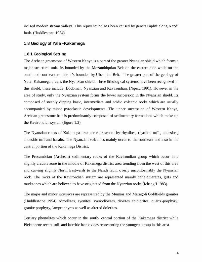
1.8 Geology of Yala –Kakamega
1.8.1 Geological Setting
The Archean greenstone of Western Kenya is a part of the greater Nyanzian shield which forms a
major structural unit. Its bounded by the Mozambiquian Belt on the eastern side while on the
south and southeastern side it’s bounded by Ubendian Belt. The greater part of the geology of
Yala- Kakamega area is the Nyanzian shield. Three lithological systems have been recognized in
this shield, these include; Dodoman, Nyanzian and Kavirondian, (Ngecu 1991). However in the
area of study, only the Nyanzian system forms the lower succession in the Nyanzian shield. Its
composed of steeply dipping basic, intermediate and acidic volcanic rocks which are usually
accompanied by minor pyroclastic developments. The upper succession of Western Kenya,
Archean greenstone belt is predominantly composed of sedimentary formations which make up
the Kavirondian system (figure 1.3).
The Nyanzian rocks of Kakamega area are represented by rhyolites, rhyolitic tuffs, andesites,
andesitic tuff and basalts. The Nyanzian volcanics mainly occur to the southeast and also in the
central portion of the Kakamega District.
The Precambrian (Archean) sedimentary rocks of the Kavirondian group which occur in a
slightly arcuate zone in the middle of Kakamega district area trending from the west of this area
and curving slightly North Eastwards to the Nandi fault, overly unconformably the Nyanzian
rock. The rocks of the Kavirondian system are represented mainly conglomerates, grits and
mudstones which are believed to have originated from the Nyanzian rocks,(Ichang’i 1983).
The major and minor intrusives are represented by the Mumias and Maragoli Goldfields granites
(Huddlestone 1954) admellites, syenites, syenodiorites, diorites epidiorites, quartz-porphyry,
granite porphyry, lamprophyres as well as altered dolerites.
Tertiary phonolites which occur in the south- central portion of the Kakamega district while
Pleistocene recent soil and lateritic iron oxides representing the youngest group in this area.

5
Mineralization in the greenstone belt consists of gold in association with silver both of which
occurs mostly in small quartz veins or reefs, lead, zinc and copper in the form of
sulphides(galena, sphalerite and chalcopyrite.) (Pulfrey 1952).
1.8.2 Structural Geology
The metamorphic effect encountered in the rocks are to a greater part as a result of thermal
metamorphism due to Mumias granite and diorite intrusions (Pulfrey 1946). He was able to
delineate two major metamorphic zones in the Nyanzian volcanic rocks in the Maragoli Region
these are Hornblende zone and Hornblende Biotite zone.
Most of the area is underlain by sedimentary rocks of the Kavirondian system and these have
approximately East – West strike lines over most of the area. The sedimentary rocks have been
folded approximately along East-West fold axes and dips are on average high ranging from 50°
to almost vertical generally (figure 1.2) towards the north and south (Ichang’I 1981).
mudstone
grit
(………….)
conglomeratte
rhyolite
Granite intrusive
Basement rock
Figure 1.2 Geological Cross section of the region. (Huddlestone 1954)

6
Figure 1.3 Geological map of Yala – Kakamega area. (Barongo 1987)
N
7
CHAPTER 2
2.1 BASIC PRINCIPLES
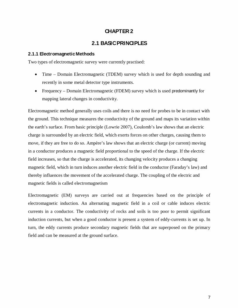
2.1.1 Electromagnetic Methods
Two types of electromagnetic survey were currently practised:
Time – Domain Electromagnetic (TDEM) survey which is used for depth sounding and
recently in some metal detector type instruments.
Frequency – Domain Electromagnetic (FDEM) survey which is used predominantly for
mapping lateral changes in conductivity.
Electromagnetic method generally uses coils and there is no need for probes to be in contact with
the ground. This technique measures the conductivity of the ground and maps its variation within
the earth’s surface. From basic principle (Lowrie 2007), Coulomb’s law shows that an electric
charge is surrounded by an electric field, which exerts forces on other charges, causing them to
move, if they are free to do so. Ampère’s law shows that an electric charge (or current) moving
in a conductor produces a magnetic field proportional to the speed of the charge. If the electric
field increases, so that the charge is accelerated, its changing velocity produces a changing
magnetic field, which in turn induces another electric field in the conductor (Faraday’s law) and
thereby influences the movement of the accelerated charge. The coupling of the electric and
magnetic fields is called electromagnetism
Electromagnetic (EM) surveys are carried out at frequencies based on the principle of
electromagnetic induction. An alternating magnetic field in a coil or cable induces electric
currents in a conductor. The conductivity of rocks and soils is too poor to permit significant
induction currents, but when a good conductor is present a system of eddy-currents is set up. In
turn, the eddy currents produce secondary magnetic fields that are superposed on the primary
field and can be measured at the ground surface.

8
Fig 2.1 (a) Primary and secondary fields in the horizontal loop induction method. (b) Amplitudes
and phases of the primary (p) and secondary (s) fields. (Lowrie 2007)
2.1.1.1 Frequency Domain E.M Method
To illustrate the concept involved, consider the simplified figure 2.1 above. Each of the three
coils represent a particular agreement of an actual E.M system. The transmitter generates the
primary field at a fixed frequency. The conducting loop represents an idealized geological
conductor in the subsurface, with resistance (R) and self-inductance (L), while the receiver loop
measures the resulting magnetic fields. Each loop is coupled to the others by mutual inductance.
For a fixed frequency, let (ep) represents the induced voltage in the receiver caused by the direct
coupling to the transmitter, while (es) represents the induced voltage in the receiver caused by
secondary field created by the ground loop.
The ratio of (es) to (ep) voltages or ratio of HS/HP in the receiver is a measure of the response
from the ground conductor necessarily normalized to offset any variance in the primary field
strength as observed at the receiver.
In frequency domain surveys, alternating currents are passed through transmitter loop or wire at
frequencies 200-4000HZ. There will, in general be a phase difference between the primary and
secondary fields and anomalies are normally expressed in terms of amplitude of the secondary
field (es) competent that are in IN PHASE and QUADRATURE (out of phase by 90°) with the
9
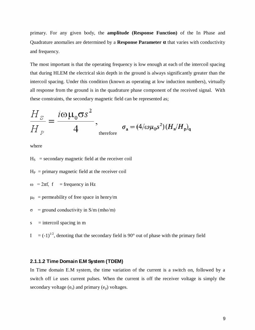
primary. For any given body, the amplitude (Response Function) of the In Phase and
Quadrature anomalies are determined by a Response Parameter α that varies with conductivity
and frequency.
The most important is that the operating frequency is low enough at each of the intercoil spacing
that during HLEM the electrical skin depth in the ground is always significantly greater than the
intercoil spacing. Under this condition (known as operating at low induction numbers), virtually
all response from the ground is in the quadrature phase component of the received signal. With
these constraints, the secondary magnetic field can be represented as;
therefore
where
HS = secondary magnetic field at the receiver coil
HP = primary magnetic field at the receiver coil
ω = 2πf, f = frequency in Hz
μ0 = permeability of free space in henry/m
σ = ground conductivity in S/m (mho/m)
s = intercoil spacing in m
I = (-1)1/2, denoting that the secondary field is 90° out of phase with the primary field
2.1.1.2 Time Domain E.M System (TDEM)
In Time domain E.M system, the time variation of the current is a switch on, followed by a
switch off i.e uses current pulses. When the current is off the receiver voltage is simply the
secondary voltage (es) and primary (ep) voltages.

10
The secondary voltage shows the characteristic exponential decay of an LR circuit, that is to say,
the rate of decay depends on the resistance (R) and inductance (L) of the ground. In general good
conductors have secondary field responses which decay slowly after switch off. These good
conductors can be detected at great depth when the conductor is large and the intervening
material is highly resistive. Poor conductors have responses that decay rapidly.
Figure 2.2 transmitter current pulse and current decay after current is switched off. (Lowrie
2007)

11
CHAPTER 3
3.0 METHODOLOGY Geophysical exploration of VMS involves reconnaissance survey to search for areas where
mineralization occurs. This is followed by detailed survey to pinpoint or delineate the VMS
mineralization.
Reconnaissance Survey
Time Domain Airbone EM.
Vertical Loop EM. (VLEM)
Detailed Survey
Horizontal Loop EM. (HLEM)
3.1 TIME DOMAIN AIRBORNE EM METHOD
Controlled source airborne EM survey systems were developed after the Second World War to
explore for mineral deposits to respond primarily to conductivity of material in the earth
(Richard 2010). Their primary success by International Nickel Company in early fifties was
discovering highly conductive massive sulphide bodies located in resistive terrain in Canada.
3.1.1 Field Proceedures.
The receiver is towed behind and below the aircraft. These systems have a transmitting coil
mounted around the aircraft giving a large dipole moment usually around 105Am2. Typically
they have a large transmitting- receiving coil separation (75-100m) and flying at an altitude of
100-150m above ground level at an approximate speed of 160 to 180km/hr. A flight path is
determined by describing the flight line and line spacing for the aircraft navigation. Extraneous
EM noise produced by man-made and natural signals eg radio waves, electric power lines quite
often pose severe problems. Therefore most EM signals should be fitted with 50 or 60 HZ to
counteract this effect.
In late 1977, a combined electromagnetic/magnetic airborne geophysical survey was flown in the
greenstone belt of Western Kenya by Terra survey limited of Ottawa, Canada on behalf of the

12
Kenyan Government. This was a reconnaissance survey to locate possible areas of anomalous or
mineralization. A towed bird time domain input MKV system was used. The survey area was
divided into five blocks covering a total area of about 4000km2. The flight line spacing in all
blocks was 200m except for some extensions with a line spacing of 500m. a total of
approximately 18600 line km were flown at an average terrain clearance of 1200m (Barongo
1987).
Figure 3.1 Airbone EM Survey plan. (Lowrie 2007)
From basic principle a current pulse is transmitted and the transient EM response is measured
after the pulse is turned off.
The input AEM system samples the anomaly decay curve at 6 different time windows and
records then on six channels. Therefore a complete input AEM anomaly would contain bars or
signature of at most 6 different characters. The bars with dark shading represents an anomaly that
shows on all six channels. Anomaly recorded on only one channel is represented by two parallel
dashed lines.
The higher the number of channels a particular anomaly shows the higher the conductance or
conductivity thickness product of the conductor the bar represents. A group of enclosed bars or
signatures represents an input AEM anomaly which in turn delineates a conductive zone in the
ground.
13
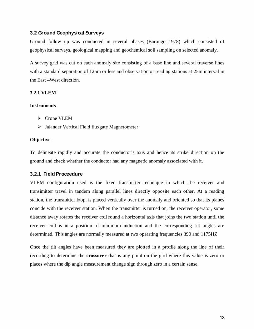
3.2 Ground Geophysical Surveys
Ground follow up was conducted in several phases (Barongo 1978) which consisted of
geophysical surveys, geological mapping and geochemical soil sampling on selected anomaly.
A survey grid was cut on each anomaly site consisting of a base line and several traverse lines
with a standard separation of 125m or less and observation or reading stations at 25m interval in
the East –West direction.
3.2.1 VLEM
Instruments
Crone VLEM
Jalander Vertical Field fluxgate Magnetometer
Objective
To delineate rapidly and accurate the conductor’s axis and hence its strike direction on the
ground and check whether the conductor had any magnetic anomaly associated with it.
3.2.1 Field Proceedure
VLEM configuration used is the fixed transmitter technique in which the receiver and
transimitter travel in tandem along parallel lines directly opposite each other. At a reading
station, the transmitter loop, is placed vertically over the anomaly and oriented so that its planes
concide with the receiver station. When the transmitter is turned on, the receiver operator, some
distance away rotates the receiver coil round a horizontal axis that joins the two station until the
receiver coil is in a position of minimum induction and the corresponding tilt angles are
determined. This angles are normally measured at two operating frequencies 390 and 1175HZ
Once the tilt angles have been measured they are plotted in a profile along the line of their
recording to determine the crossover that is any point on the grid where this value is zero or
places where the dip angle measurement change sign through zero in a certain sense.

14
Figure 3.2 (a) Plan view of VLEM field procedure (b) strike direction of a conductor. (Melvyne
1989)
3.2.2 HLEM
The horizontal loop EM system used consist of a consist of a transmitting coil and a receiver.
The transmitter generates a frequency which is usually set between 200Hz and 4000Hz. This
signal is detected by the receiving coil and a cable connecting the transmitter and receiver allows
the signal to be completely cancelled when no geological conductor is present. If a conducting
body is present the transmitted signal will generate eddy current in that body. These eddy
currents in turn generate a secondary magnetic field which is detected and measured by the
receiving coil. It is customary to measure the component in phase with the primary transmitted
signal and that which lags it by 90° (quadrature)
Instruments
Apex Max MinII HLEM System
3.2.2.1 Field procedure
The transmitter (Tx) and receiver (Rx) coils remain in coplanar configuration at constant
seperations. When surveying the Tx and Rx coupled by the reference cable move as a unit long
the traverse line (figure 3.3). Intervals reading are taken at one quarter the coil separation. When
an anomalous response is encountered, readings are often closed up to one eighth the coil
separation to provide greater density of data to aid in its definition.
crossover
15
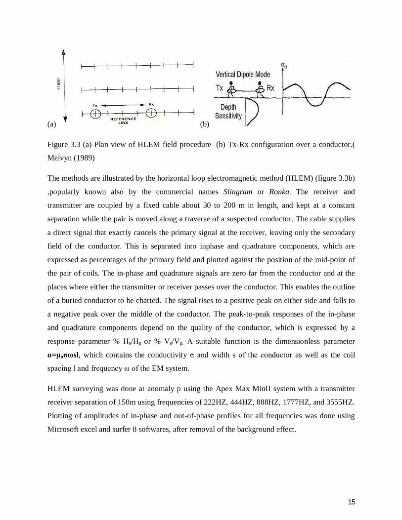
(a) (b)
Figure 3.3 (a) Plan view of HLEM field procedure (b) Tx-Rx configuration over a conductor.(
Melvyn (1989)
The methods are illustrated by the horizontal loop electromagnetic method (HLEM) (figure 3.3b)
,popularly known also by the commercial names Slingram or Ronka. The receiver and
transmitter are coupled by a fixed cable about 30 to 200 m in length, and kept at a constant
separation while the pair is moved along a traverse of a suspected conductor. The cable supplies
a direct signal that exactly cancels the primary signal at the receiver, leaving only the secondary
field of the conductor. This is separated into inphase and quadrature components, which are
expressed as percentages of the primary field and plotted against the position of the mid-point of
the pair of coils. The in-phase and quadrature signals are zero far from the conductor and at the
places where either the transmitter or receiver passes over the conductor. This enables the outline
of a buried conductor to be charted. The signal rises to a positive peak on either side and falls to
a negative peak over the middle of the conductor. The peak-to-peak responses of the in-phase
and quadrature components depend on the quality of the conductor, which is expressed by a
response parameter % Hs/Hp or % Vs/Vp. A suitable function is the dimensionless parameter
α=μoσωsl, which contains the conductivity σ and width s of the conductor as well as the coil
spacing l and frequency ω of the EM system.
HLEM surveying was done at anomaly p using the Apex Max MinII system with a transmitter
receiver separation of 150m using frequencies of 222HZ, 444HZ, 888HZ, 1777HZ, and 3555HZ.
Plotting of amplitudes of in-phase and out-of-phase profiles for all frequencies was done using
Microsoft excel and surfer 8 softwares, after removal of the background effect.

16
Figure 3.4 (a) Geometry of an HLEM profile across a thin vertical dike. (b) In-phase and
quadrature profiles over a dike for some values of the dimensionless response parameter a.
(Lowrie 2007)

17
CHAPTER 4
4.0 RESULTS and INTERPRETATION
4.1 Results
4.1.1 Reconnaissance AEM RESULTS
Two sets of input AEM anomaly maps figure 4.1 and figure 4.2 were prepared at a scale of
1:25000 and 1:50000. In these maps the airborne anomalies are represented by groups of
enclosed EM signatures in the form of parallel or semi-parallel thin bars with or without a
pointer in the middle. The extent of each bar or signature marks the extent of a conductor along
a particular flight line. As the input AEM system samples the anomaly decay curves at six
different time windows and records them on six channels, a complete input AEM anomaly map
would contain bars or signatures of at most six different characters.
The bars with dark shading represent an anomaly that shows on all six channels of the input
AEM record. The other bars have a decreasing intensity of shading related to the number of
channels on which the anomaly is recorded. An anomaly recorded on only one channel is
represented by two parallel dashed lines. The higher the number of channels a particular anomaly
shows on, the higher the conductance or conductivity-thickness product σt (where σ is the
conductivity and t is the thickness). A group of enclosed bars or signatures represents an input
AEM anomaly which in turn delineates a conductive zone on the ground.
4.1.2 Interpretation
Applying the convectional criteria for selecting conductor anomalies due to massive sulphide
bodies namely; conductance, magnetic association, and conductor isolation a priority rating of
(1-3) is assigned to most probable bedrock for the purpose of ground follow up.
After ground follow up through geochemistry and ground geophysics and geology, the rating is
modified based on high conductance, favourable geology and presence of mineral outcrops to
select potential targets for further study.
Figure 4.2 shows the location of the four input AEM anomalies and the geology in which they
occur. Anomaly P is wholly situated in the mafic geology of the Kavirondian system dominated
by mudstones. Anomaly Q occurs on or near the boundary between the Nyanzian andesites and

18
rhyolites and the Kavirondian conglomerates and grits. Anomaly R in the felsic and highly
resistive rhyolitic geology of the Nyanzian system while anomaly S, which occurs on the
boundary between the Nyanzian rhyolites and andesites.
Figure 4.1 location of EM anomalies P,Q,R, and S. (Barongo 1987)

19
Figure 4.2 Geology of the area containing EM anomalies P,Q,R, and S (Barongo 1987)
20
An interesting correlation between the anomaly map and geology is observed. Figure 4.2 shows
that about one third of the area to the northwest is covered by elongated anomalies that coincide
well with the area covered by Nyanzian andesites while the regions covered by granitic
intrusives show no anomalies. The regions covered by Kavirondian conglomerates, grit and
mudstone show no anomalies.
4.1.3 Detailed Ground Survey Results
Ground geophysical survey which involved Vertical loop EM (VLEM) to delineate the strike of
the conductor and Horizontal loop EM (HLEM) to determine the depth and thickness of the ore
conductor. However, only anomaly P was taken into consideration in this report since they offer
substantial information.
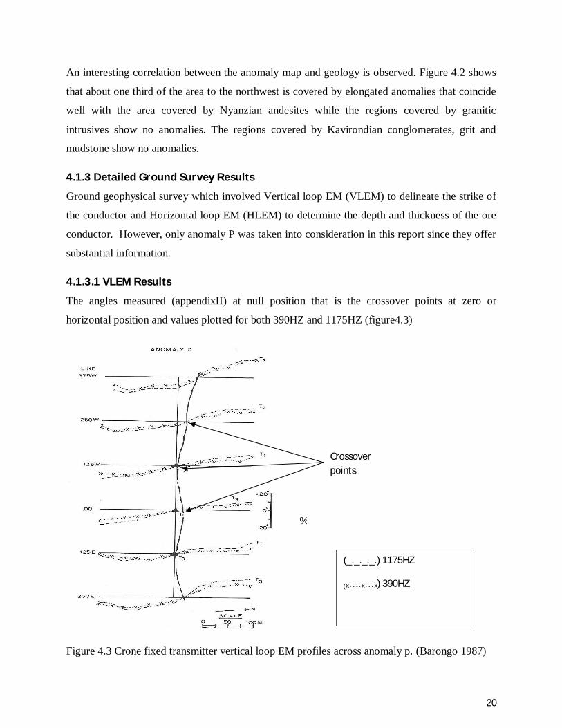
4.1.3.1 VLEM Results
The angles measured (appendixII) at null position that is the crossover points at zero or
horizontal position and values plotted for both 390HZ and 1175HZ (figure4.3)
Figure 4.3 Crone fixed transmitter vertical loop EM profiles across anomaly p. (Barongo 1987)
%
Crossover points
(_._._._.) 1175HZ
(X…..X….X) 390HZ
21
4.1.3.2 Interpretation
The trace of the conductor is found by joining the crossover points from one traverse line to the
next (figure 4.3). The strike is found to be roughly to the east – west direction. There is a
correlation between the geological structures and the strike- dip direction. From previous
mineralization the VMS deposits occur as stratiform deposits that is horizontally parallel to the
rock structures. However due to metamorphism as discussed in the geology its evident that the
VMS have been folded together with other rocks and occur now as sheeted dykes. Anomaly Q
occurs in the same latitude or horizon with anomaly P hence they have same strike.
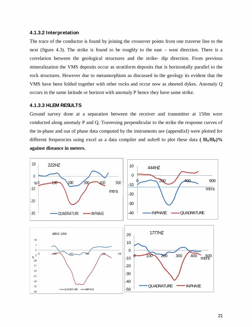
4.1.3.3 HLEM RESULTS
Ground survey done at a separation between the receiver and transmitter at 150m were
conducted along anomaly P and Q. Traversing perpendicular to the strike the response curves of
the in-phase and out of phase data computed by the instruments see (appendixI) were plotted for
different frequencies using excel as a data compiler and sufer8 to plot these data ( HS/HP)%
against distance in meters.
-40
-30
-20
-10
0
10
0 200 400 600
INPHASE QUADRATURE
444HZ
mtrs
-50
-40
-30
-20
-10
0
10
20
0 100 200 300 400 500
QUADRATURE INPHASE
1777HZ
mtrs
222HZ
mtrs %
mtrs

22
-50
-40
-30
-20
-10
00 100 200 300 400 500
QUADRATURE INPHASE
3555HZ
Figure 4.4 HLEM profiles for frequencies 222HZ, 444HZ, 888HZ, 1777HZ and 3555HZ.
4.1.3.4 Interpretation
The anomaly curves observed for the HLEM measurements show a significant response at the
location of the buried ore conductor. At low frequencies of 222HZ and 444HZ, significant
anomalies are observed especially on the in-phase component. At high frequencies however,
there is a general gradual increase particularly on in-phase amplitude due to the skin depth effect
discussed in chapter two.
The profiles also show a common symmetrical shape more on the in-phase component. This
indicates that the ore body is vertical or has a 90° dip. This is supported from the calculation of
dip based on the ratio of the areas under the two shoulders of the curve (A1/A2) in which it
varies from one for a symmetrical, vertical case to zero for a horizontal sheet (John 1997).
-40
-30
-20
-10
0
10
0 100 200 300 400 500 600
INPHASE QUADRATURE
444HZ
mtrs A1 A
Ratio
=1.35
DIP =89.9°

23
Figure 4.5 Calculation of dip of ore body.
Free-air phasor diagrams of Nair Biwas and Mazumdar (1968) in appendixIII are used to
calculate the values of depth to the top of the conductor (d) and its conductivity thickness
product σt.
222HZ 444HZ 888HZ 1777HZ 3555HZ
In-Phase -15.79 -21.32 -27.43 -31.54 -37.14
Quardrature -8.67 -8.90 -6.13 -6.90 -8.43
d (depth) m 45.0 39.0 37.5 35.0 22.5
σt (s) 53.2 37.5 34.0 35.0 12.3
Table 4.1 interpreted results from the HLEM profiles of anomalyP.
The table below shows the thickness of the ore body calculated as the difference between the two
shoulder distances.
Frequency
Hz
222 444 888 1777 3555
Thickness (m) 246.1 300 275 271 223
Average
Thickness
263.0m
Table 4.2 interpreted thickness from the HLEM profiles of anomaly P.

24
0 50 100 150 200 250 300 350 400METERS
-5
AN
OM
AL
Y
-23-22-21-20-19-18-17-16-15-14-13-12-11-10-9-8-7-6-5-4
Figure 4.6 (a) A drill hole of anomaly s at 310w traverse line. (Barongo 1987) (b) An interpreted
contour anomaly map.
A contour map showing the anomaly with red indicating anomalies while blue shows
background or host rock plotted for all frequencies, plotted using surfer8 software.
VMS CONTOUR ANOMALY MAP
VMS SHEETED DYKE

25
CHAPTER 5
5.0 DISCUSSION CONCLUSION AND RECOMMENDATION
5.1 DISCUSSION The electromagnetic method is effective in locating and detecting shallow VMS deposits. It is
observed that the VMS deposits are found at shallow depth with an average value of 40 meters
deep, and a thickness of about 263m. Upon drilling (figure 4.6a) shows mineralization to be
composed of pyrite and graphite.
It is observed that the input airborne EM response is much more common in the areas underlain
by andesites and rhyolites than any other rock type (figure 4.2). The area covered by granitic
intrusives is completely bare of these anomalies. This correlation can be useful in geological
mapping.
Mineralogy of VMS states that they occur as stratiform deposits. However from dip calculation
and strike delineation, the VMS occur as a sheeted dyke. In context, metamorphism caused
folding and dipping of host rocks to nearly vertical positions (Huddleston 1954) hence stratiform
layers were oriented almost vertically to form sheeted dykes. This is evidenced by the presence
of graphite which forms under extreme temperature and pressure.
It is observed that the effect of conductive overburden in galvanic contact with a target conductor
(VMS) affects the EM response at high frequencies. Tropical environment has a conductive
upper zone due to water and weathering products such as clays which interfere with the EM
response as frequencies increases. The overall effect makes the target conductor appear shallow
and less conductive at higher frequencies. (Mwanifembo 1997).
5.2 Conclusion The geophysical techniques are very important tools in the imaging the subsurface. Its accuracy
and simplicity makes electromagnetic technique very efficient and cheap. The geology and
structures are important in locating these deposits. VMS deposits occur mainly in felsic extrusive
igneous rocks such as rhyolites and andesites. These rock types are good location areas for VMS
deposits. The structures are important in delineating their occurrence and give vital information
on how to mine them.
26
5.3 Recommendation
VMS deposits are source of base metals and gold and from the study , they occur at
shallow depths. These deposits therefore can be excavated easily and cheaply.
The greenstone belt extends for miles into Tanzania. These are areas of potential VMS
deposits which should be surveyed using the EM technique and anomaly maps be
sketched for further detailed geophysical studies.
The VMS deposits are associated by submarine environments (Alan 2007). Kenya hosts
the Mozambique Belt which is a collision zone, closing up an ocean (Prichard and
Alabaster 1993). Therefore VMS deposits have a potential of being hosted in these areas.
Geophysical techniques need to be embraced in each county if they are to locate and
manage their own geological resources.

27
REFERENCES Alan G. Galley and Hannington M.D and Jonasson J.R (2007), Volcanogenic Massive
Sulphide Deposits, Mineral Deposit of Canada; A Synthesis of Major Deposit Type and
Exploration Methods, Geological Association of Canada, Special Publication No. 5, pg
141-161.
Barongo J.O (1987), Geophysical Detection of Mineral of Mineral Conductors in
Tropical Terrains with Target Conductors Partly Embedded in the Conductive
Overbudden, pg 3-17.
Huddelson A. (1954), Geology of the Kakamega District, Report No. 28, pg 2-14.
Ichang’I W. Daniel (1983), The Bukura and Mbesa Pyrite Mineralization of Western
Kenya, MSC thesis UON, pg 41-48.
John M. Reynolds (1997), An Introduction to Applied and Environmental Geophysics,
John wiley and Sons publishers, England, pg 550-568.
Lowrie William (2007), Fundamentals of geophysics, 2nd edition, Cambridge University
Press, New York, pg 258 – 300.
Melvyne Best and John B. Borniwell (1989), A Geophysical Handbook for Geologist,
Vol 41, Canada, pg 199-220.
Mwenifumbo C.J (1997), Electrical Methods for Ore Body Delineation, Proceeding of
Exploration 97: Fourth Decinnal international Conference of Mineral Exploration, pg
667-676.
Ngecu M. Wilson (1991), The geology of Kavirondian Group of Sediments, Thesis UON
pg 3-26.
Prichard, H. M, Alabaster T and Neary C. R (1993), Magmatic Processes and Plate
Tectonic, Geological Society special Publication No. 76, pg 345-362.
Pulfrey William (1952), Geology of Kisumu District, Report No. 21, Pg 5-15.
Richard Smith (2010), Airborne Electromagnetic Methods Applications to Minerals,
Water and Hydrocarbon Exploration, Lecture tour, Laurentian University Canada, pg 1-6.
Telford W.M (2001), Applied Geophysics, 2nd edition, Cambridge university Press
Publishers UK, Pg 380-381.
http://www.mapcruzin.com/free-maps-kenya/kenya_sm_2008.gif accessed on 5th May 2011.
28
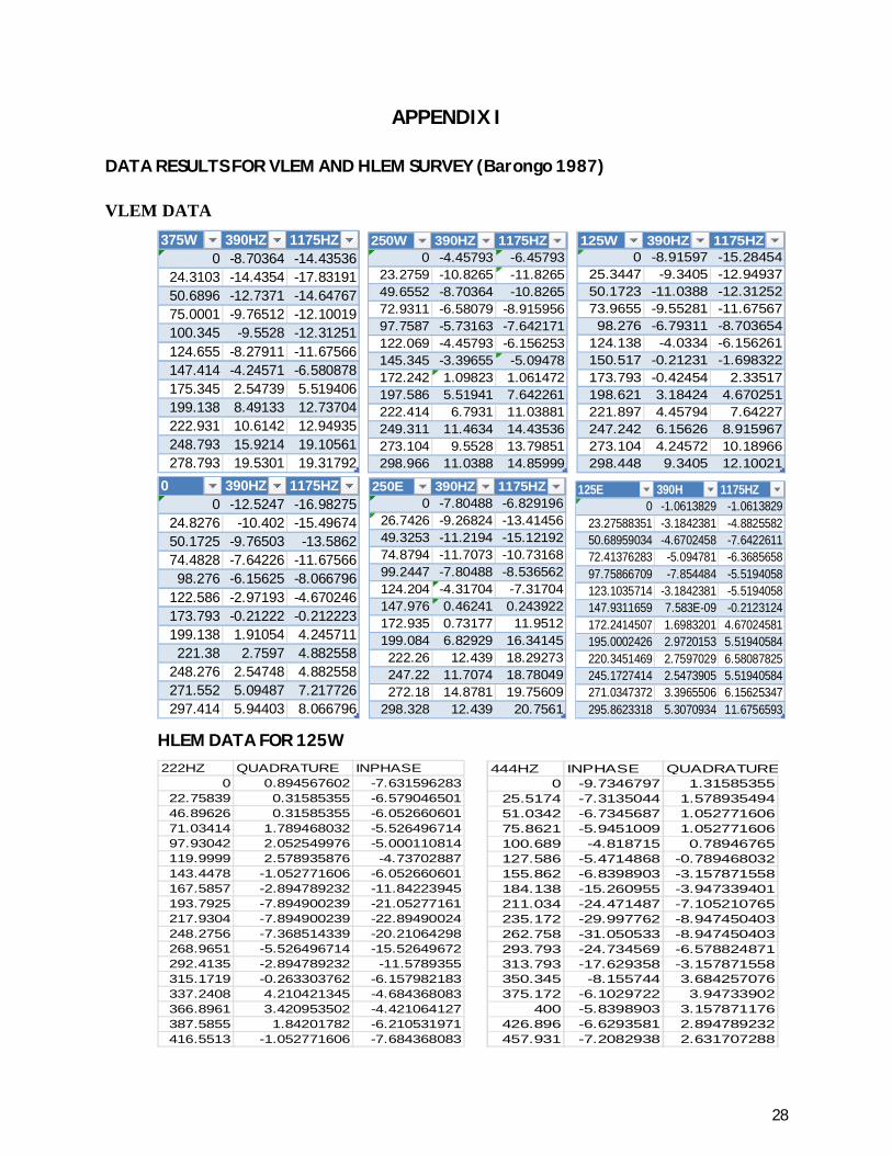
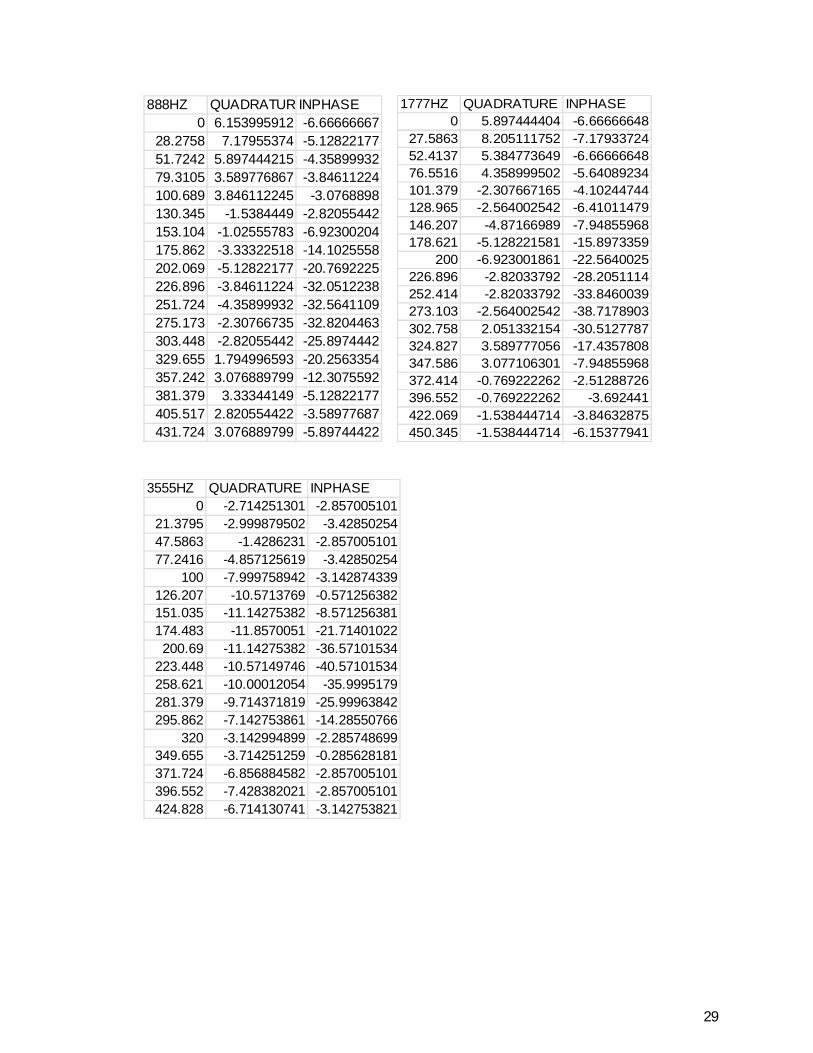
APPENDIX I
DATA RESULTS FOR VLEM AND HLEM SURVEY (Barongo 1987)
VLEM DATA 375W 390HZ 1175HZ
0 -8.70364 -14.4353624.3103 -14.4354 -17.8319150.6896 -12.7371 -14.6476775.0001 -9.76512 -12.10019100.345 -9.5528 -12.31251124.655 -8.27911 -11.67566147.414 -4.24571 -6.580878175.345 2.54739 5.519406199.138 8.49133 12.73704222.931 10.6142 12.94935248.793 15.9214 19.10561278.793 19.5301 19.31792
250W 390HZ 1175HZ0 -4.45793 -6.45793
23.2759 -10.8265 -11.826549.6552 -8.70364 -10.826572.9311 -6.58079 -8.91595697.7587 -5.73163 -7.642171122.069 -4.45793 -6.156253145.345 -3.39655 -5.09478172.242 1.09823 1.061472197.586 5.51941 7.642261222.414 6.7931 11.03881249.311 11.4634 14.43536273.104 9.5528 13.79851298.966 11.0388 14.85999
125W 390HZ 1175HZ0 -8.91597 -15.28454
25.3447 -9.3405 -12.9493750.1723 -11.0388 -12.3125273.9655 -9.55281 -11.6756798.276 -6.79311 -8.703654
124.138 -4.0334 -6.156261150.517 -0.21231 -1.698322173.793 -0.42454 2.33517198.621 3.18424 4.670251221.897 4.45794 7.64227247.242 6.15626 8.915967273.104 4.24572 10.18966298.448 9.3405 12.10021
0 390HZ 1175HZ0 -12.5247 -16.98275
24.8276 -10.402 -15.4967450.1725 -9.76503 -13.586274.4828 -7.64226 -11.6756698.276 -6.15625 -8.066796
122.586 -2.97193 -4.670246173.793 -0.21222 -0.212223199.138 1.91054 4.245711221.38 2.7597 4.882558
248.276 2.54748 4.882558271.552 5.09487 7.217726297.414 5.94403 8.066796
250E 390HZ 1175HZ0 -7.80488 -6.829196
26.7426 -9.26824 -13.4145649.3253 -11.2194 -15.1219274.8794 -11.7073 -10.7316899.2447 -7.80488 -8.536562124.204 -4.31704 -7.31704147.976 0.46241 0.243922172.935 0.73177 11.9512199.084 6.82929 16.34145222.26 12.439 18.29273247.22 11.7074 18.78049272.18 14.8781 19.75609
298.328 12.439 20.7561
125E 390H 1175HZ0 -1.0613829 -1.0613829
23.27588351 -3.1842381 -4.882558250.68959034 -4.6702458 -7.642261172.41376283 -5.094781 -6.368565897.75866709 -7.854484 -5.5194058123.1035714 -3.1842381 -5.5194058147.9311659 7.583E-09 -0.2123124172.2414507 1.6983201 4.67024581195.0002426 2.9720153 5.51940584220.3451469 2.7597029 6.58087825245.1727414 2.5473905 5.51940584271.0347372 3.3965506 6.15625347295.8623318 5.3070934 11.6756593
HLEM DATA FOR 125W 222HZ QUADRATURE INPHASE
0 0.894567602 -7.63159628322.75839 0.31585355 -6.57904650146.89626 0.31585355 -6.05266060171.03414 1.789468032 -5.52649671497.93042 2.052549976 -5.000110814119.9999 2.578935876 -4.73702887143.4478 -1.052771606 -6.052660601167.5857 -2.894789232 -11.84223945193.7925 -7.894900239 -21.05277161217.9304 -7.894900239 -22.89490024248.2756 -7.368514339 -20.21064298268.9651 -5.526496714 -15.52649672292.4135 -2.894789232 -11.5789355315.1719 -0.263303762 -6.157982183337.2408 4.210421345 -4.684368083366.8961 3.420953502 -4.421064127387.5855 1.84201782 -6.210531971416.5513 -1.052771606 -7.684368083
444HZ INPHASE QUADRATURE0 -9.7346797 1.31585355
25.5174 -7.3135044 1.57893549451.0342 -6.7345687 1.05277160675.8621 -5.9451009 1.052771606100.689 -4.818715 0.78946765127.586 -5.4714868 -0.789468032155.862 -6.8398903 -3.157871558184.138 -15.260955 -3.947339401211.034 -24.471487 -7.105210765235.172 -29.997762 -8.947450403262.758 -31.050533 -8.947450403293.793 -24.734569 -6.578824871313.793 -17.629358 -3.157871558350.345 -8.155744 3.684257076375.172 -6.1029722 3.94733902
400 -5.8398903 3.157871176426.896 -6.6293581 2.894789232457.931 -7.2082938 2.631707288
29
888HZ QUADRATUREINPHASE0 6.153995912 -6.66666667
28.2758 7.17955374 -5.1282217751.7242 5.897444215 -4.3589993279.3105 3.589776867 -3.84611224100.689 3.846112245 -3.0768898130.345 -1.5384449 -2.82055442153.104 -1.02555783 -6.92300204175.862 -3.33322518 -14.1025558202.069 -5.12822177 -20.7692225226.896 -3.84611224 -32.0512238251.724 -4.35899932 -32.5641109275.173 -2.30766735 -32.8204463303.448 -2.82055442 -25.8974442329.655 1.794996593 -20.2563354357.242 3.076889799 -12.3075592381.379 3.33344149 -5.12822177405.517 2.820554422 -3.58977687431.724 3.076889799 -5.89744422
1777HZ QUADRATURE INPHASE0 5.897444404 -6.66666648
27.5863 8.205111752 -7.1793372452.4137 5.384773649 -6.6666664876.5516 4.358999502 -5.64089234101.379 -2.307667165 -4.10244744128.965 -2.564002542 -6.41011479146.207 -4.87166989 -7.94855968178.621 -5.128221581 -15.8973359
200 -6.923001861 -22.5640025226.896 -2.82033792 -28.2051114252.414 -2.82033792 -33.8460039273.103 -2.564002542 -38.7178903302.758 2.051332154 -30.5127787324.827 3.589777056 -17.4357808347.586 3.077106301 -7.94855968372.414 -0.769222262 -2.51288726396.552 -0.769222262 -3.692441422.069 -1.538444714 -3.84632875450.345 -1.538444714 -6.15377941
3555HZ QUADRATURE INPHASE
0 -2.714251301 -2.85700510121.3795 -2.999879502 -3.4285025447.5863 -1.4286231 -2.85700510177.2416 -4.857125619 -3.42850254
100 -7.999758942 -3.142874339126.207 -10.5713769 -0.571256382151.035 -11.14275382 -8.571256381174.483 -11.8570051 -21.71401022200.69 -11.14275382 -36.57101534
223.448 -10.57149746 -40.57101534258.621 -10.00012054 -35.9995179281.379 -9.714371819 -25.99963842295.862 -7.142753861 -14.28550766
320 -3.142994899 -2.285748699349.655 -3.714251259 -0.285628181371.724 -6.856884582 -2.857005101396.552 -7.428382021 -2.857005101424.828 -6.714130741 -3.142753821
30
APPENDIX II
VLEM GRAPHICAL RESULTS
375W
250W
125W
00
125E
250E
CROSSOVERS

31
APPENDIX III
FREE-AIR PHASOR DIAGRAMS
Free-air phasor diagrams of Nair Biwas and Mazumdar (1968) (Telford 2001)