Geophysical Journal InternationalGeophys. J. Int. (2016) 207, 89–110 doi: 10.1093/gji/ggw257Advance Access publication 2016 July 14GJI Gravity, geodesy and tides

Elastic tidal response of a laterally heterogeneous planet: a completeperturbation formulation

Chuan Qin, Shijie Zhong and John WahrDepartment of Physics, University of Colorado at Boulder, Boulder, CO 80309, USA. E-mail: chuan.qin@colorado.edu

Accepted 2016 July 8. Received 2016 July 8; in original form 2016 April 2

S U M M A R YConstraining laterally varying structures in planetary interiors is important for understandingboth the composition and the internal dynamics of a planet. Recognizing that seismic imagingtechnique is currently only viable for studying the Earth’s interior structures, methods thatcan be supported by advanced space geodetic techniques may become alternatives to ‘im-age’ the interiors of other planets. The method of tidal tomography is one possibility, and itrelies on high precision measurement of the response of a planet to its body tide. However,it is essential to develop an efficient analytical tool that computes the dependence of tidalresponse to 3-D interior structures. In this paper, we present a complete formulation of suchan analytical tool, which calculates to high accuracy the tidal response of a terrestrial planetwith lateral heterogeneities in its elastic and density structures. We treat the lateral hetero-geneities as small perturbations and derive the governing equations based on the perturbationtheory. In a spherical harmonic representation, equations at each order of perturbation arereduced into multiple matrix equations at harmonics that are allowed by mode couplings,and the total response equals the sum of all those single-harmonic responses, which can besolved semi-analytically. We test our perturbation method by applying it to the Moon with aharmonic degree-1 mantle structure for which the perturbation solutions of the tidal responseare compared with those from a fully numerical method. The remarkable agreement betweenresults from these two methods validates the perturbation method. As an example, we then usethe perturbation method to evaluate the impact of lunar crustal thickness variations on tidalresponse of the Moon. We find that lunar crust produces much smaller degree-3 tidal responsesthan a relatively weak degree-1 structure in the deep lunar mantle. Our calculations show thatdegree-3 tidal response measurements may hold key constraints on possible degree-1 mantlestructure of the Moon, as suggested from previous modelling results.

Key words: Time variable gravity; Lunar and planetary geodesy and gravity; Tides andplanetary waves; Dynamics of lithosphere and mantle; Planetary interiors.

1 I N T RO D U C T I O N

Space observations over the past decades have revealed that some planetary bodies in the solar system have apparent long-wavelength laterallyvarying features at their surfaces. For example, the Earth’s moon displays global asymmetries in its surface chemical compositions, marebasalt volcanism and crustal thickness (e.g. Zuber et al. 1994; Smith et al. 1997; Lawrence et al. 1998; Tompkins & Pieters 1999; Lawrenceet al. 2002). Mars shows significant differences in crustal thickness between northern and southern hemispheres and in volcanism betweeneastern and western hemispheres (Zuber 2001). Mercury is proved to have a magnetic field in a north-south asymmetry, for which the surfacemagnetic field at the northern hemisphere is about three times stronger than that at the southern hemisphere (e.g. Anderson et al. 2011).The Saturn’s moon Enceladus features a geologically older northern hemisphere and a younger southern hemisphere, where an active geysersystem with abnormally high surface temperature is observed at the south-pole region (e.g. Porco et al. 2006; Spencer et al. 2006). It has beenproposed that these laterally varying features originate from the deep interiors of these planetary bodies (e.g. Zhong et al. 2000; Laneuvilleet al. 2013). Therefore, imaging the interior structures and constraining the interior material properties are crucial for understanding thecurrent state and the dynamic evolution of these bodies. However, high-resolution imaging of the planetary interiors relies on a global networkof seismometers, which are unavailable on any of the planetary bodies other than the Earth.

Advanced space geodetic techniques may provide alternative and cost-effective tools to infer the interior structure of a planetary body.The GRACE mission used a twin-satellite system to capture very small variations in the Earth’s gravity field, by measuring the position of the

C© The Authors 2016. Published by Oxford University Press on behalf of The Royal Astronomical Society. 89

90 C. Qin, S. Zhong and J. Wahr

orbiting satellites and the relative ranging rate between them at extremely high precision (Tapley et al. 2004). The later lunar mission GRAILlaunched a similar pair of twin satellites to the Moon’s low-altitude orbit and measured the Moon’s gravity field and its time-variations to anunprecedented precision (Zuber et al. 2013). The onboard LOLA (Lunar Orbiter Laser Altimeter) instrument on LRO (Lunar ReconnaissanceOrbiter) can determine the lunar global topography at high resolution and precision, and may potentially capture small ground movement ofthe lunar surface (Smith et al. 2010). These measurements and future missions open a window for using the response of a planet (i.e. changesin gravitational potential and/or surface topography) to time-varying body tide to constrain 3-D long-wavelength structure of the planetaryinterior, that is, tidal tomography (e.g. Latychev et al. 2009; Zhong et al. 2012). Tidal force acting on a planetary body with 3-D interiorstructures excites additional response modes that are distinct from those for a spherically symmetric body (1-D). In principle, the elasticresponse of a planetary body has the identical frequency as the applied time-varying tidal force, and thus is spectrally separable from the staticresponse and other low frequency responses. Although none of the above missions has so far been targeted to extract small tidal responsesignals for inference of possible 3-D interior structures, an analytical tool that can effectively compute the tidal response of a planetary bodywith 3-D interior structures is desirable.

Additionally, such an analytical tool would help improve the theoretical framework in solving general geophysical response problems.The theory and method for solving the elastic tidal/loading response of a spherically symmetric (i.e. 1-D) planetary body were establishedlong ago (Longman 1962; Longman 1963; Farrell 1972). In the following decades, response problems for a planetary body with laterallyheterogeneous material properties (i.e. 3-D) could only be solved through fully numerical methods (e.g. Latychev et al. 2009; Zhong et al.2012). Until recently, stimulated by the more advanced geodetic measurements, two different analytical tools in solving 3-D tidal responseproblems have been developed. First, motivated by the GRAIL mission, we developed a semi-analytical perturbation method based on the Lovenumber formalism that solves the elastic tidal response of a planetary body with lateral heterogeneity in the shear modulus (Qin et al. 2014).Second, Lau et al. (2015) developed a new normal mode theory that can predict the tidal response of a laterally heterogeneous, rotating andanelastic Earth in the semi-diurnal band. Their goal is to use GPS measurements of ground deformation to constrain the Earth’s deep mantlestructure. In Qin et al. (2014), we took the advantage of mathematical simplicity of the perturbation theory, and extended our formulationto the second order of perturbation for high accuracy. Systematic benchmark tests were made by comparing the perturbation solutions withthose from a finite element code (Zhong et al. 2003; A et al. 2013), showing remarkable agreement between these two solutions. However,Qin et al. (2014) only considered lateral heterogeneity in the shear modulus in their formulation and did not include lateral heterogeneities inother properties such as the first Lame parameter and the density. The benchmark calculations were only made for radial displacement andgravitational potential in the response (Qin et al. 2014).

This study is a continuation of our previous work (Qin et al. 2014). Here, we present a complete perturbation method by incorporatinglateral heterogeneities in the elastic and density structures into one formulation. Benchmarks are performed to validate our perturbationmethod, which are done not only for response in radial displacement and gravitational potential but also for that in horizontal displacement.The paper is organized as follows. In Section 2, we derive the governing equations and the perturbation formulation. A special treatment indealing with nonzero net force on the system that can potentially be caused by density anomaly is demonstrated. In Section 3, we transformour perturbation equations into a matrix form through spherical harmonic (SH) and vector spherical harmonic (VSH) expansions, and presentsolution method for solving the equations. In Section 4, we present benchmark results of tidal responses of a hemispherically asymmetric(degree-1) Moon that are computed from our perturbation method and a finite element based numerical method. We then use the perturbationmethod to calculate the tidal response of the Moon caused by the large crustal thickness variations that are inferred from the GRAILobservations. The final section is on conclusions and discussions.

2 T H E O RY

We seek to derive governing equations for tidal response of a spherically stratified planetary body superposed with small lateral heterogeneitiesin its rocky mantle and crust (hereafter, we refer to ‘mantle’ as both mantle and crust). The mantle is assumed to be compressible and respondto time-varying tidal force elastically with self-gravitational effect. We include all sources of lateral heterogeneities, which can exist in thetwo elastic moduli (shear modulus μ and first Lame parameter λ) and the density ρ. The equation of motion originates from the conservationof momentum, which is given as (Dahlen & Tromp 1998; Tromp & Mitrovica 1999b)

∇ · TE − ρE∇φE = 0, (1)

where ρE, φE and TE are Eulerian density, gravitational potential and stress field, respectively.

2.1 Background state

A spherically symmetric (1-D) planetary body is in hydrostatic equilibrium and has no deformation without external force being applied.From eq. (1), we have

∇ · T0 = ρ0∇φ0, (2)

Tidal response of a terrestrial planet 91

where ρ0, φ0 and T0 (T0 = −p0I and p0 is the hydrostatic pressure) are the reference density profile, the gravitational potential and the stressfield, respectively, and are all functions of radius. φ0 satisfies the Poisson’s equation

∇2φ0 = 4πGρ0. (3)

When there exist small lateral heterogeneities, δμ0, δλ0 and δρ0 (δμ0/μ0 � 1, δλ0/λ0 � 1 and δρ0/ρ0 � 1, where μ0, λ0 and ρ0 are1-D profiles of the shear modulus μ, the first Lame parameter λ and the density ρ, respectively), although δμ0 and δλ0 alone have no directeffect, the density anomaly δρ0 would act as a body force in causing a pre-stressed system involving mantle deformation. As a result, thispre-stressed system forms a new background state, which can be described by a new equation of motion, as

∇ · T′0 − ρ ′

0∇φ′0 = 0, (4)

where ρ ′0 = ρ0 + δρ0, φ′

0 = φ0 + δφ0, T′0 = −p0I+τ0, respectively, τ0 is the stress induced by the body force (i.e. the pre-stress), δφ0 is the

change in gravitational potential due to δρ0.It is important to note that the density-induced potential change δφ0 can no longer be determined from the Poisson’s equation ∇2δφ0 =

4πGδρ0 alone, it also contains the effect from undulations (i.e. dynamic topography) of any density interfaces in the mantle that are causedby δρ0 (e.g. Hager & Richards 1989). More generally, eq. (4) can be used to describe a system that is pre-stressed by a combined effect fromnot only internal density anomaly δρ0 but also different other sources, such as static body tide, rotation, surface loading and etc., as long asthey act in entirely different frequency bands from that of the body tide we consider. However, solving eq. (4) for a pre-stressed state mayrequire a viscous or viscoelastic rheology for the mantle, because such a flow deformation operates at a much longer time scale than theelastic tidal deformation that we consider in this study. Consequently, we ignore any pre-stress effect.

2.2 Net force due to density anomaly

The time-varying body tide may be induced by the orbital eccentricity or obliquity of the planetary body. For example, Mercury’s tide isalmost solely contributed by the Sun, and its time-dependent part is mainly caused by its orbital eccentricity. Body tide in the moons of thegas giants is predominantly raised by their planets, while the effect from the Sun and other planets is negligible. For the Earth’s Moon, thetidal potential from the Sun is ∼200 times smaller than that due to the Earth, and thus is excluded from our analyses. Also, we only considerthe leading terms in the Moon’s tidal potential that is caused by its eccentric orbit in our analyses, that is, the harmonic degree-2 terms. Wedenote the tidal potential as Vtd(t) or Vtd(r, t), so that the tidal force can be expressed as −ρ ′

0∇Vtd(t). Since Vtd(t) is at degree-2 SHs, theresponse of a spherically symmetric (1-D) body would be at the same harmonics. However, when coupled with laterally heterogeneous (3-D)structures, the degree-2 tidal force also excites non-degree-2 harmonics in the response.

In principle, solving tidal response of a planetary body requires external forces be balanced, which means the net external force on thesystem must be equal to zero. On a spherically symmetric (1-D) body, the tidal force −ρ0∇Vtd(t) never causes a net force. However, whendensity anomaly δρ0 is present, the coupling term −δρ0∇Vtd(t) may result in a nonzero net force on the planetary body. Physically, this netforce would only accelerate the planetary body but not cause any deformation. However, keeping this net force in the term −δρ0∇Vtd(t) andincluding it in the equation of motion would impose an incorrect force balance on the system, leading to errors in the solutions. To correctlysolve the tidal response, we remove this net force component by redefining the problem in a non-inertial reference frame which is acceleratingwith the planetary body. A fictitious inertial force is added in the equation of motion as to cancel the net force, as discussed below.

Mode coupling in the forcing term −δρ0∇Vtd(t) can be solved by VSH expansion that will be introduced in Section 3. In the expansionform,

−δρ0∇Vtd(t) =∑l,m

f l,m(r, t), (5)

where f l,m(r, t) is the modal component at harmonic (l, m). It can be mathematically proved that only a harmonic degree-1 modal componentcan cause a nonzero net force. We thus focus on the degree-1 components in eq. (5), which can be further expressed as

f 1,m(r, t) = f P1,m(r, t)P1,m + f B

1,m(r, t)B1,m, (6)

where P1,m and B1,m are VSH basis functions for a spheroidal vector (see Section 3) of degree 1 and order m of 1, 0 or −1, and f P1,m and

f B1,m are the expansion coefficients for corresponding basis functions. We compute the net force f net(t) by integrating f 1,m(r, t) throughout

the mantle, as

f net(t) =�

V

f 1,m(r, t)r 2 sin θdrdθdφ. (7)

The direction of f net(t) depends on the choice of m and

f net(t) =

⎧⎪⎪⎨⎪⎪⎩

f0(t)x m = 1

f0(t) y m = −1

f0(t) z m = 0

, (8)

92 C. Qin, S. Zhong and J. Wahr

where x, y and z are unit vectors in Cartesian coordinates, and

f0(t) = 4π

3

a∫rcmb

[f P1,m(r, t) + 2 f B

1,m(r, t)]

r 2 dr , (9)

where rcmb and a are the radii of the core–mantle boundary (CMB) and the surface, respectively. f net(t) would accelerate the planet with theacceleration

atot(t) = f net(t)

M, (10)

where M is the total mass of the planet.Solving degree-1 deformation in the accelerating reference requires an inertial force be added to every portion of the mantle, where the

inertial force is equal to

f int(r, t) = −ρ ′0atot(t) = −ρ ′

0

f0(t)

M(P1,m + B1,m), (11)

which is in the opposite direction of the acceleration. Here we make use of the following relation in eq. (11).

P1,m + B1,m =

⎧⎪⎪⎨⎪⎪⎩

x m = 1

y m = −1

z m = 0

. (12)

2.3 Governing equations

The time-varying tidal force −ρ0′∇Vtd(t) deforms the pre-stressed mantle elastically further by u(t), in addition to any background deformation.

As a result, the equation of motion is updated to

∇ · [T′0 + TE1(t)] − [ρ ′

0 + ρE1(t)]∇[φ′0 + Vtd(t) + ϕE1(t)] − ρ ′

0atot(t) = 0, (13)

where ρE1(t), ϕE1(t) and TE1(t) are Eulerian perturbations in density, gravitational potential and stress, respectively, due to the incrementaldeformation u(t), and the inertial force f int = −ρ ′

0atot is added to cancel potential nonzero net force on the planet. Subtracting eq. (4) (i.e.the background state) from eq. (13) and neglecting small terms involving products of Eulerian increments lead to the linearized governingequation for tidal response, which is given by

∇ · TE1(t) − ρ ′0∇[Vtd(t) + ϕE1(t)] − ρE1(t)∇φ′

0 − ρ ′0atot(t) = 0. (14)

Note that we have ignored the effect of pre-stress τ0 for linearization of eq. (14) as usually done in formulation for similar analyses (e.g.Dahlen & Tromp 1998; Tromp & Mitrovica 1999a). Considering δφ0 � φ0, we will also neglect the effect of δφ0 in eq. (14).

We substitute the Eulerian incremental stress TE1(t) with the Lagrangian form through the relation (Dahlen & Tromp 1998)

TE1(t) = TL1(t) − u(t) · ∇T0, (15)

where TL1(t) can be related to u(t) through the constitutive relation by assuming simple elasticity for the mantle, as

TL1 = TL1(λ′0, μ

′0, u) = λ′

0(∇ · u)I+μ′0(∇u + ∇Tu), (16)

where μ′0 = μ0 + δμ0 and λ′

0 = λ0 + δλ0. We obtain the final equation of motion as

∇ · TL1(λ′0, μ

′0, u) − ∇(ρ0u · ∇φ0) − ρ ′

0∇(Vtd + ϕE1) − ρE1∇φ0 − ρ ′0atot = 0, (17)

and together with the Poisson’s equation

∇2ϕE1 = 4πGρE1, (18)

where the Eulerian density perturbation ρE1 is related to u through

ρE1 = −∇ · (ρ ′0u). (19)

Note that u, ϕE1, TL1 and atot all have the same time dependence as the tidal potential Vtd(t). Here, we can omit the time dependence ineqs (16)–(19) for elastic response.

Compared with the governing equations in Qin et al. (2014), eqs (16)–(19) also include the effects of δλ0 and δρ0 on the response,together with that of δμ0. If δμ0, δλ0 and δρ0 vanish, eqs (16)–(19) would automatically reduce to the 1-D equations that reconcile eqs (1)–(3)in Qin et al. (2014). Hereafter, we omit any superscripts that denote an Eulerian or Lagrangian quantity.

Tidal response of a terrestrial planet 93

2.4 Perturbation formulation

Solving eqs (16)–(19) for u and ϕ fully determines the tidal response. We solve the equations using a perturbation method, in which we treat anysmall lateral heterogeneities (3-D) in the mantle as perturbations to the 1-D reference state (similar to what Qin et al. (2014) used in modelling3-D structures in shear modulus μ). We denote the tidal response solution for the 1-D reference structure as (u0, ϕ0) and the solution for thatbeing perturbed by a 3-D structure as (u, ϕ). The difference between the two solutions, denoted as (u′, ϕ′)[i.e. (u′, ϕ′) = (u, ϕ) − (u0, ϕ0)],represents the incremental tidal response as a result of the 3-D structure. Taking (u0, ϕ0) as zeroth order solution, we further divide (u′, ϕ′)into high order solutions by the order of perturbation in the lateral heterogeneities to represent incremental responses at different levels ofaccuracy, as (u′, ϕ′) = (u1, ϕ1) + (u2, ϕ2) + (u′′, ϕ′′), where (u1, ϕ1), (u2, ϕ2) and (u′′, ϕ′′) are called first order, second order and residual(higher than second order) solutions, respectively (Qin et al. 2014). Since a second order approximation to (u, ϕ) is sufficiently accurate, wedrop (u′′, ϕ′′) and replace u and ϕ in eqs (16)–(19) with u0 + u1 + u2 and ϕ0 + ϕ1 + ϕ2, respectively. As a result, different orders of solutions(up to second order of perturbation) are grouped into individual sets of perturbation equations, which can be expressed in a generalized formas

∇ · TD − ∇(ρ0uD · ∇φ0) − ρ0∇ϕD + ∇ · (ρ0uD)∇φ0 = −FD, (20)

∇2ϕD + 4πG∇ · (ρ0uD) = −GD, (21)

TD = λ0(∇ · uD)I+μ0(∇uD + ∇TuD), (22)

where FD and GD are called the coupling terms, the subscript D indicates the order of perturbation and can be 0, 1 or 2, that is, the zeroth,first or second order. Eqs (20)–(22) have non-trivial solutions only when the coupling termFD or GD is non-zero.

When D = 0 (i.e. zeroth order), F0 = −ρ0∇Vtd and G0 = 0, and eqs (20)–(22) solves the tidal response for a spherically symmetric(1-D) body. The technique in solving 1-D response was well developed decades ago (Longman 1962; Longman 1963; Farrell 1972).Difficulties lie in solving the higher order equations, that is for D = 1 or 2, due to involvement of the coupling terms. At higher orders,FD = Fμ

D +FλD +Fρ

D , whereFμ

D ,FλD andFρ

D are mutually independent and are contributions toFD from the coupling between the lowerorder (D − 1) solution and the lateral heterogeneities δμ0, δλ0 and δρ0, respectively, as seen from

Fμ

D = ∇ · [δμ0(∇uD−1 + ∇TuD−1)], (23)

FλD = ∇(δλ0∇ · uD−1), (24)

Fρ

D = −δρ0∇ϕD−1 + ∇ · (δρ0uD−1)∇φ0 + f ρ

D . (25)

Note that Fμ

D and FλD keep the same form in different orders of equations, while Fρ

D differs by an extra term f ρ

D between the first and thesecond orders. Specifically,

f ρ

1 = −δρ0∇Vtd − ρ0atot, (26)

f ρ

2 = −δρ0atot. (27)

Also, at higher orders,

GD = 4πG∇ · (δρ0uD−1), (28)

and GD is non-zero only when δρ0 �= 0.Solving eqs (20)–(22) requires appropriate continuity conditions as well as boundary conditions at the outer surface and the CMB (e.g.

Qin et al. 2014). Across any concentric interface in the spherically layered mantle, uD , ϕD , the normal traction term (r · TD+BD) and thepotential gradient term [r · (∇ϕD + 4πGρ0uD) +HD] must be continuous, which can be expressed as

[uD]+− = [ϕD]+− = [r · TD+BD

]+− = [

r · (∇ϕD + 4πGρ0uD) +HD

]+− = 0, (29)

where []+− symbolizes the jump of the enclosed quantity across an interface, r is the normal vector in the radial direction, BD and HD aretwo other coupling terms. Specifically, BD is induced by δμ0 or δλ0 while HD results from δρ0, and both of them are non-zero only in thehigher order equations (i.e. D = 1 or 2). SplittingBD into terms that represent δμ0 and δλ0 contributions, asBD = Bμ

D +Bλ

D ,Bμ

D ,Bλ

D andHD are given by

Bμ

D = r · [δμ0(∇uD−1 + ∇TuD−1)], (30)

Bλ

D = r · [δλ0(∇ · uD−1)I] , (31)

HD = r · 4πGδρ0uD−1, (32)

respectively. The surface and CMB boundary conditions are provided in the next section in a matrix form.

94 C. Qin, S. Zhong and J. Wahr

3 M E T H O D

We solve the perturbation equations, that is eqs (20)–(22), through a two-step procedure (Qin et al. 2014). Step one: we perform SH and VSHexpansions, respectively, for any 3-D scalars and vectors that enter in the perturbation equations. In this way, a complete set of harmonic modesin the tidal response solution can be pre-determined by solving the mode coupling terms. Meanwhile, any radially dependent component ofthe solution is separated from the angular dependence in the harmonics, thus reducing the problem of solving the partial differential equations(i.e. eqs 20–22) into solving multiple sets of ordinary differential equations (ODEs) with respect to the radius that are associated with theharmonics allowed by the mode couplings. Each set of ODEs can then be converted into a more manageable matrix form for solution (Dahlen& Tromp 1998; Tromp & Mitrovica 1999b). Step two: we adopt the propagator matrix method to solve those resulting matrix equations foreach response mode from each order of perturbation. The total response is equal to the sum of all those responses.

Eqs (20)–(22) and the corresponding continuity and boundary conditions are non-dimensionalized by the following scalings:

r = ar , uD = auD, ϕD = 4πGρcmba2ϕD, ∇ = 1

a∇,

μ0 = μcmbμ0, λ0 = μcmbλ0, ρ0 = ρcmbρ0,

δμ0 = μcmbδμ0, δλ0 = μcmbδλ0, δρ0 = ρcmbδρ0,

TD = μcmbTD,FD = μcmb

aFD,BD = μcmbBD,

GD = 4πGρcmbGD,HD = 4πGρcmbaHD, (33)

where the tilt denotes a non-dimensional quantity, a is the radius of the planet, ρcmb and μcmb are the reference density and shear modulus rightabove the CMB, respectively. Thus, the non-dimensional form of the perturbation equations [i.e. eqs (20)–(22)] and the associated continuityconditions [eq. (29)] are expressed as

∇ · TD − η[∇(ρ0uD · ∇φ0) + ρ0∇ϕD − ∇ · (ρ0uD)∇φ0

] = −FD, (34)

∇2ϕD + ∇ · (ρ0uD) = −GD, (35)

TD = λ0(∇ · uD)I+μ0(∇ uD + ∇TuD), (36)

[uD]+− = [ϕD]+− =[r · TD+BD

]+

−=[r · (∇ϕD + ρ0uD) + HD

]+

−= 0, (37)

respectively, where η = 4πGρ2cmba2

μcmb, FD = Fμ

D + FλD + ηFρ

D and BD = Bμ

D + BλD . Hereafter, all the quantities are non-dimensional and we

omit the tilts for brevity.We expand all 3-D scalar and vector variables in the spherical coordinates (r, θ, φ) into SHs and VSHs, respectively, of which the basis

functions are (Dahlen & Tromp 1998; Tromp & Mitrovica 1999b)

Ylm = Ylm(θ, φ), P lm = rYlm, Blm = ∇1Ylm, C lm = r × ∇1Ylm, (38)

where Ylm is the SH function in real form, P lm , Blm and C lm are vector functions defined over (θ, φ), l and m are harmonic degree and order,respectively, which define a unique mode in the harmonics. The explicit expressions of these basis functions are given in appendix A of Qinet al. (2014). Assuming that the lateral heterogeneities are composed of eigenstructures of different SHs, they can be expanded into

δμ0 =∑l1,m1

μ

l1m1(r )μ0(r )Yl1m1 (θ, φ), (39)

δλ0 =∑l1,m1

λl1m1

(r )λ0(r )Yl1m1 (θ, φ), (40)

δρ0 =∑l1,m1

ρ

l1m1(r )ρ0(r )Yl1m1 (θ, φ), (41)

respectively, where l1m1 (r ) measures the lateral variability of the heterogeneities and is considered to be small.uD , ϕD and r · TD are expanded respectively into (Dahlen & Tromp 1998; Tromp & Mitrovica 1999b)

uD =∑l,m

(U D

lm P lm + V Dlm Blm + W D

lm C lm

), (42)

ϕD =∑l,m

K DlmYlm, (43)

r · TD =∑l,m

(RD

lm P lm + SDlm Blm + T D

lm C lm

), (44)

Tidal response of a terrestrial planet 95

where the expansion coefficients are functions of radius. The expansion coefficients U Dlm , V D

lm , W Dlm and K D

lm fully describe the tidal responsesolution at mode (l, m) and order D. RD

lm , SDlm , T D

lm and an auxiliary variable Q Dlm are derivative terms, which are given specifically by (Dahlen

& Tromp 1998; Tromp & Mitrovica 1999b)

RDlm = (λ0 + 2μ0)U D

lm + λ0

r

(2U D

lm − l(l + 1)V Dlm

), (45)

SDlm = μ0

(V D

lm − V Dlm

r+ U D

lm

r

), (46)

T Dlm = μ0

(W D

lm − W Dlm

r

), (47)

Q Dlm = K D

lm + l + 1

rK D

lm + ρ0U Dlm, (48)

where a dot denotes the first order derivative with respect to radius.The mode coupling terms FD , GD , BD and HD (for D > 0) need to be expanded into appropriate forms in order for the high-order

responses to be solved. Here, we only show the symbolic expansion forms of these terms, as

FD =∑l,m

(F p,D

lm P lm + Fb,Dlm Blm + Fc,D

lm C lm

), (49)

GD =∑l,m

G DlmYlm, (50)

BD =∑l,m

(B p,D

lm P lm + Bb,Dlm Blm + Bc,D

lm C lm

), (51)

HD =∑l,m

H DlmYlm, (52)

where D = 1 or 2, while their full expressions are given in Appendix A and will enter in the matrix equations before the propagator matrixmethod being applied. Note that determining the coupling terms at order D requires that the response at order D − 1 be fully solved. Thecoupling terms govern the response modes at each order of perturbation (for D > 0) through the selection rule [eq. (22) in Qin et al. (2014)].A permissible mode in the response is indicated by a non-trivial set of expansion coefficients ofFD ,BD ,HD and GD at that specific mode.Thus, tidal response is restricted to a finite number of pre-determined modes other than spans in infinite number of modes. More descriptionsof the mode coupling can be referred to section 3.2 of Qin et al. (2014).

The SH and VSH expansion forms (i.e. eqs 39–52) help turn the perturbation equations at order D (eqs 20–22) into equations forindividual response modes, and these equations can be further reduced to ODEs with respect to radius by dropping angular dependence inthe harmonics. The ODEs of a single mode belong to either one of the two categories: spheroidal (s) and toroidal (t), which describe twonon-overlapping sets of components in the response. The spheroidal (s) component includes all the vector components that span in P lm andBlm , and potential and potential derivatives; the toroidal component only includes vector components in C lm . We can convert these ODEsinto a matrix form, and the spheroidal and toroidal equations share the same general form, as

dX Dlm

dr= Al X D

lm − FDlm, (53)

where X Dlm is the solution vector of mode (l, m), Al is a square matrix and depends on l but not on m or D, and FD

lm is the vectorized form ofthe two coupling termsFD and GD . The explicit forms of X D

lm , Al and FDlm as well as the associated continuity and boundary conditions are

different for spheroidal and toroidal modes. Specifically,

(1) Spheroidal mode

X Dlm = (

U Dlm, V D

lm, RDlm, SD

lm, K Dlm, Q D

lm

)T. (54)

Al =

⎛⎜⎜⎜⎜⎜⎜⎜⎜⎜⎜⎜⎝

− 2λ0rβ

l(l+1)λ0rβ

1β

0 0 0

− 1r

1r 0 1

μ00 0

4r ( γ

r − ξ ) − l(l+1)r ( 2γ

r − ξ ) − 4μ0rβ

l(l+1)r − ξ (l+1)

g0rξ

g0

1r (ξ − 2γ

r ) − 1r2 [2μ0 − l(l + 1)(γ + μ0)] − λ0

rβ − 3r

ξ

rg00

−ρ0 0 0 0 − l+1r 1

−ρ0l+1

r ρ0l(l+1)

r 0 0 0 l−1r

⎞⎟⎟⎟⎟⎟⎟⎟⎟⎟⎟⎟⎠

, (55)

96 C. Qin, S. Zhong and J. Wahr

where β = λ0 + 2μ0 , γ = μ0(3λ0+2μ0)λ0+2μ0

, ξ = ηρ0g0 and η = 4πGρ2cmba2

μcmb.

FDlm =

(0, 0, F p,D

lm , Fb,Dlm , 0, G D

lm

)T. (56)

The vectorized continuity conditions in the solid mantle and the boundary conditions are, respectively,[U D

lm

]+− = [

V Dlm

]+− = [

K Dlm

]+− =

[RD

lm + B p,Dlm

]+

−= [

SDlm + Bb,D

lm

]+− = [

Q Dlm + H D

lm

]+− = 0, (57)

X Dlm(rcmb) =

(U D

lm, V Dlm, ηρ0

(K D

lm+g0U Dlm

), 0, K D

lm,2l + 1

rcK D

lm + ρ0U Dlm

)T

r=rcmb

, (58)

X Dlm(a) = (U D

lm, V Dlm, 0, 0, K D

lm, 0)Tr=a, (59)

where X Dlm(rcmb) and X D

lm(a) are solution vectors at the CMB and the outer surface, respectively.

(2) Toroidal mode

X Dlm = (

W Dlm, T D

lm

)T. (60)

Al =(

1r

1μ0

(l+2)(l−1)μ0r2 − 3

r

). (61)

FDlm = (

0, Fc,Dlm

)T. (62)

The associated continuity conditions and boundary conditions are[W D

lm

]+− = [

T Dlm + Bc,D

lm

]+− = 0, (63)

X Dlm (rcmb) = (

W Dlm, 0

)T

r=rcmb, (64)

X Dlm(a) = (

W Dlm, 0

)T

r=a, (65)

respectively.Solving eqs (16)–(19) for the total tidal response (u, ϕ), up to second order accuracy in the perturbation, is now equivalent to summing

over the responses of all the individual modes at every order of perturbation. The relative magnitude of the response is only a function of thelateral variabilities in the heterogeneities (see Appendix A). In addition, response at each mode is a combined effect of the three sources oflateral heterogeneities (i.e. those in μ, λ and ρ). As a direct consequence of our perturbation formulation, the first order response is simplythe sum of the first order responses induced by individual sources, that is, only one source of lateral heterogeneity appears while the othertwo are zeroed out. This can be shown as

X1lm = X1,μ

lm + X1,λlm + X1,ρ

lm , (66)

where X1,μ

lm , X1,λlm and X1,ρ

lm (X2,μ

lm , X2,λlm and X2,ρ

lm for later) are first order (second order) solutions due to lateral heterogeneity only in μ, λ andρ, respectively. This summation rule, however, does not hold for the second order responses. The first order solution X1

lm would enter in thesecond order coupling terms (see eqs 23–28 and 30–32), resulting in X2,μ

lm , X2,λlm , X2,ρ

lm as well as cross effects between the lateral heterogeneitiesinto the second order solution X2

lm , as

X2lm = X2,μ

lm + X2,λlm + X2,ρ

lm +(χ

δμ⊗δλ

lm + χδμ⊗δρ

lm + χδλ⊗δρ

lm

), (67)

where the symbol ⊗ represents the cross effects between two lateral heterogeneities.We implement the propagator matrix method based on a fourth order Runge–Kutta numerical scheme to solve the whole set of matrix

equations, mode by mode, from zeroth to second order of perturbation. The implementation of the propagator matrix method can be referredto section 3.3 and appendix C in Qin et al. (2014). The whole solution procedure of the perturbation method is summarized in Appendix B.

4 R E S U LT S

In this section, we use the perturbation method to calculate the tidal response of a laterally heterogeneous planetary body. As we did in ourprevious study (Qin et al. 2014), we continue to apply our method to the Earth’s moon, of which the long-wavelength structure in depth isstill unknown. But compared to other planetary bodies, we have a much better constraint on the Moon’s 1-D reference profile (Weber et al.2011) as well as its 3-D structure at shallow depths, for example, lunar crustal thickness variations (e.g. Wieczorek et al. 2013).

Tidal response of a terrestrial planet 97

The Moon has a clear hemispherical asymmetry in its surface geological settings, for example, mare volcanism (e.g. Wieczorek et al.2006) and crustal thickness (e.g. Wieczorek et al. 2013). Those asymmetries may have originated from a deeper source of long-wavelengthheterogeneities, from a dynamic point of view (e.g. Zhong et al. 2000; Laneuville et al. 2013). More interestingly, recent analyses on deepseismicity in the lunar interior (Nakamura 2005) imply that those potential heterogeneities may have partially survived the thermochemicalevolution and remain in the present-day lunar mantle (Qin et al. 2012). One mechanism predicts that those potential mantle heterogeneities,if existed, may have the same asymmetric distribution as that near the surface, which is a nearside-farside antipodal distribution (Qin et al.2012). This mantle structure can be described predominantly by a (1, 1) SH in certain depth range in our chosen coordinate system (i.e. theorigin of the coordinate system is fixed at the centre of the Moon, with x-axis pointing towards the sub-Earth point and z-axis perpendicularto the Moon’s orbital plane). Considering such (1, 1) structure in the elastic moduli and the density, we have

δμ0 = μ

1,1(r )μ0(r )Y1,1 = −δμ

1,1(r )μ0(r ) sin θ cos φ, (68)

δλ0 = λ1,1(r )λ0(r )Y1,1 = −δλ

1,1(r )λ0(r ) sin θ cos φ, (69)

δρ0 = ρ

1,1(r )ρ0(r )Y1,1 = −δρ

1,1(r )ρ0(r ) sin θ cos φ, (70)

where Y1,1 = −√

34π

sin θ cos φ, 1,1 is called the lateral variability, δ1,1 measures the amplitude of the (1, 1) lateral variability and δ1,1 =√3

4π1,1. In general, 1,1(r ) is piecewise constant as a function of the radius.In the following calculations, we select the time-varying part of the tidal potential that is due to the eccentricity of the Moon’s orbit, and

only consider the leading harmonic degree-2 terms [Wahr et al. 2009; eq. (4) in Qin et al. (2014)]. In a simplified form, the tidal potential isgiven by

Vtd(r, t) = [�2,0(r )Y2,0 + �2,2(r )Y2,2

]T (t), (71)

which contains both (2, 0) and (2, 2) components. T (t) represents the time dependence of the tidal potential, which can be dropped whensolving elastic tidal response.

For a 1-D planetary body, tidal response can be fully described by three non-dimensional Love numbers (Love 1911). The tidal responseis spheroidal and the solution (i.e. for D = 0) can be expressed by⎡⎢⎢⎣

U 0l0m0

(r )

V 0l0m0

(r )

K 0l0m0

(r )

⎤⎥⎥⎦ = �td

l0m0(r )

⎡⎢⎢⎣

hl0 (r )/g0

ll0 (r )/g0

kl0 (r )

⎤⎥⎥⎦ , (72)

where (l0, m0) denotes the harmonic of a specific potential term, hl0 , ll0 and kl0 are tidal Love numbers, which represent responses in radialdisplacement, horizontal displacement and gravitational potential, respectively. The Love numbers depend only on the 1-D reference profileand the harmonic degree (Love 1911; Farrell 1972). For a planetary body with 3-D structure, additional (high order) responses due to themode coupling occur at multiple harmonics (l, m)’s in either spheroidal or toroidal mode. For each mode at order of perturbation D, wenon-dimensionalize the tidal response solution based on eq. (72), and normalize it further by the three Love numbers. As a result, we get

hD′lm (r ) = U D

lm(r )

U 0l0m0

(r ), l D′

lm (r ) = V Dlm(r )

V 0l0m0

(r ), k D′

lm (r ) = K Dlm(r )

K 0l0m0

(r ), wD′

lm (r ) = W Dlm(r )

V 0l0m0

(r ), (73)

where hD′lm , l D′

lm and k D′lm (wD′

lm ) are called relative responses of a spheroidal (toroidal) mode s D(l, m) [t D(l, m)]. Note that hD′lm , l D′

lm , k D′lm and wD′

lm

can be positive or negative values. At the zeroth order, h0′l0m0

= l0′l0m0

= k0′l0m0

≡ 1, and w0′l0m0

does not exist.We now use our perturbation method to do the following calculations. First, we run benchmark calculations to verify the formulation

and implementation of the perturbation method for lateral heterogeneities in elastic structures, similar to the benchmark cases in Qin et al.(2014) (see table 1 in Qin et al. (2014) for the 1-D reference model of the Moon). The benchmark is done by comparing solutions from ourperturbation method with those from a finite element method (Zhong et al. 2012; A et al. 2013; Qin et al. 2014). Second, since the finiteelement solutions are not yet available for cases with lateral heterogeneity in density, we calculate the density effect on the tidal response andcompare it with the effect from lateral heterogeneity in shear modulus. Third, we evaluate the impact of lunar crustal thickness variations onthe tidal response.

4.1 Benchmarks

In Qin et al. (2014), benchmarks were performed for cases in which (1, 1) lateral heterogeneity exists purely in the shear modulus μ. Here,we first apply the same procedure on (1, 1) lateral heterogeneity in first Lame parameter λ, by comparing the tidal response solutions fromthe perturbation method and the finite element method (Zhong et al. 2003; A et al. 2013). For benchmark purposes, the responses to (2, 0)and (2, 2) tidal forcing components are computed separately, such that the relative magnitude of the forcing needs not to be considered. Alsofor simplicity, we set the amplitudes of lateral variability in elastic and density structures, that is, δ

μ

1,1, δλ1,1 and δ

ρ

1,1, to be constant throughoutthe lunar mantle (i.e. independent of the radius).

98 C. Qin, S. Zhong and J. Wahr

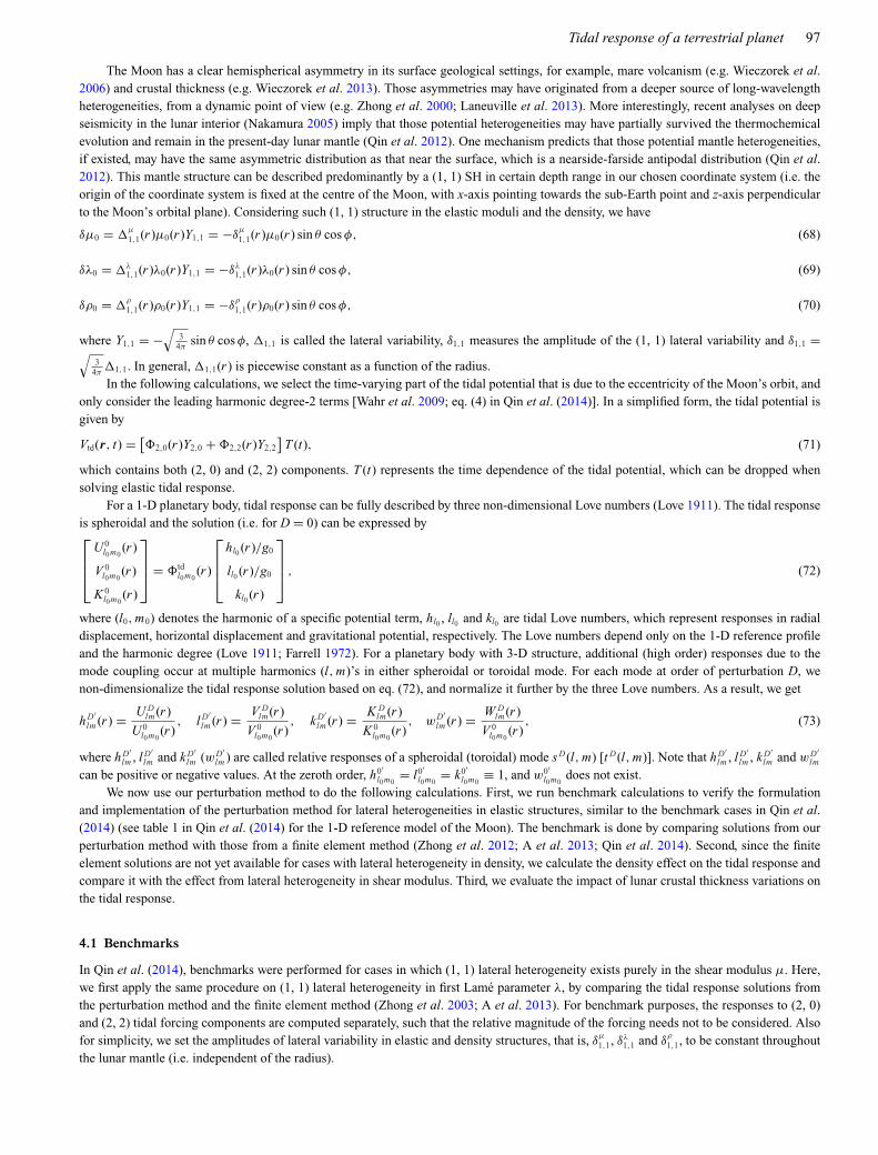
Figure 1. Hierarchies of mode couplings (up to order of perturbation D = 2) between spherical harmonic (1, 1) lateral heterogeneity in shear modulus μ, firstLame parameter λ or density ρ and (2, 0) (a) and (2, 2) (b) tidal forcing, respectively. s or t denotes a spheroidal or toroidal mode, and superscript 0, 1 or 2denotes order of perturbation D. The dashed boxes and lines mark the toroidal modes and the couplings that are associated with toroidal modes, respectively,which are allowed in μ and ρ cases but prohibited in λ case.

We first show the mode coupling diagrams to the second order of perturbation for (2, 0) and (2, 2) tidal forcing in Figs 1(a) and (b),respectively. The selection rule [eq. (22) in Qin et al. (2014)] holds the same for δμ0, δλ0 and δρ0, except that δλ0 does not induce anytoroidal modes as δμ0 and δρ0 do. This said, we obtain the same set of spheroidal modes in the response from different sources of (1, 1)lateral heterogeneity, but the toroidal modes t1(2, −1) and t2(3, −2) and the mode couplings that are associated with them (marked by dashedframes and lines in Fig. 1) do not exist for δλ0 case.

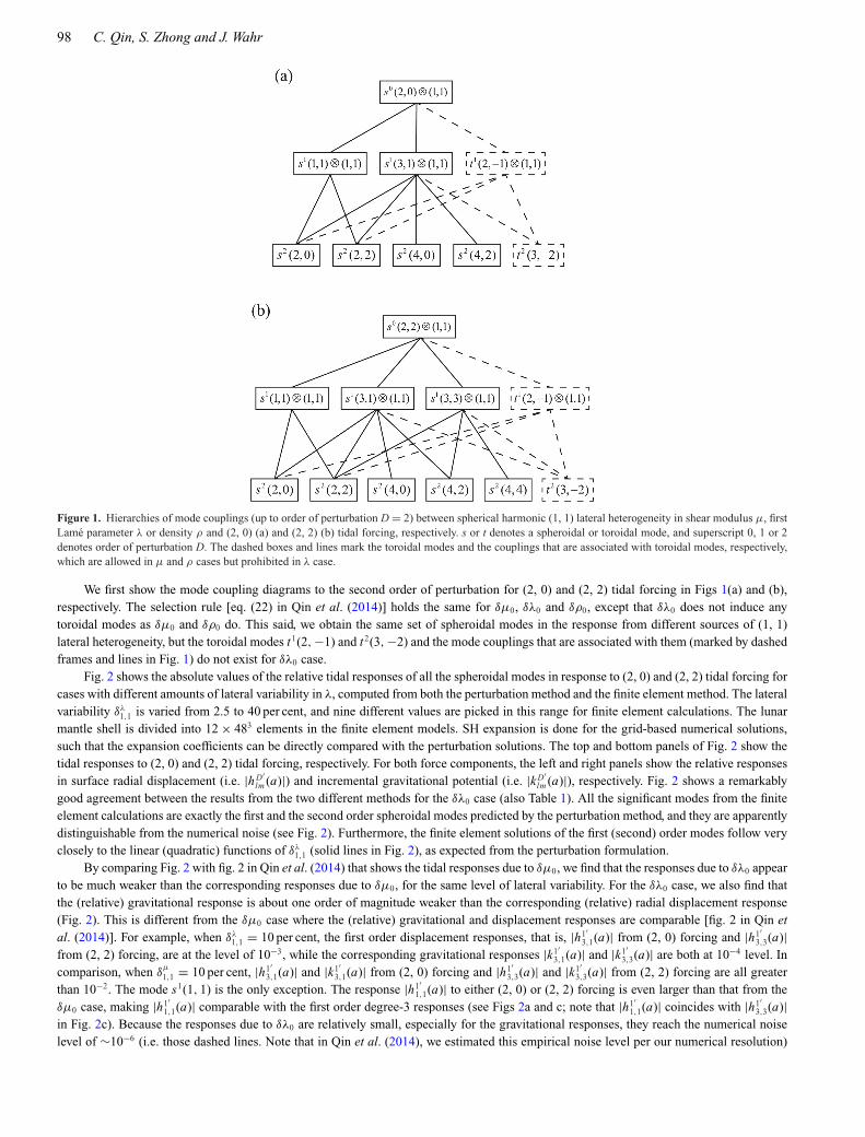
Fig. 2 shows the absolute values of the relative tidal responses of all the spheroidal modes in response to (2, 0) and (2, 2) tidal forcing forcases with different amounts of lateral variability in λ, computed from both the perturbation method and the finite element method. The lateralvariability δλ

1,1 is varied from 2.5 to 40 per cent, and nine different values are picked in this range for finite element calculations. The lunarmantle shell is divided into 12 × 483 elements in the finite element models. SH expansion is done for the grid-based numerical solutions,such that the expansion coefficients can be directly compared with the perturbation solutions. The top and bottom panels of Fig. 2 show thetidal responses to (2, 0) and (2, 2) tidal forcing, respectively. For both force components, the left and right panels show the relative responsesin surface radial displacement (i.e. |hD′

lm (a)|) and incremental gravitational potential (i.e. |k D′lm (a)|), respectively. Fig. 2 shows a remarkably

good agreement between the results from the two different methods for the δλ0 case (also Table 1). All the significant modes from the finiteelement calculations are exactly the first and the second order spheroidal modes predicted by the perturbation method, and they are apparentlydistinguishable from the numerical noise (see Fig. 2). Furthermore, the finite element solutions of the first (second) order modes follow veryclosely to the linear (quadratic) functions of δλ

1,1 (solid lines in Fig. 2), as expected from the perturbation formulation.By comparing Fig. 2 with fig. 2 in Qin et al. (2014) that shows the tidal responses due to δμ0, we find that the responses due to δλ0 appear

to be much weaker than the corresponding responses due to δμ0, for the same level of lateral variability. For the δλ0 case, we also find thatthe (relative) gravitational response is about one order of magnitude weaker than the corresponding (relative) radial displacement response(Fig. 2). This is different from the δμ0 case where the (relative) gravitational and displacement responses are comparable [fig. 2 in Qin etal. (2014)]. For example, when δλ

1,1 = 10 per cent, the first order displacement responses, that is, |h1′3,1(a)| from (2, 0) forcing and |h1′

3,3(a)|from (2, 2) forcing, are at the level of 10−3, while the corresponding gravitational responses |k1′

3,1(a)| and |k1′3,3(a)| are both at 10−4 level. In

comparison, when δμ

1,1 = 10 per cent, |h1′3,1(a)| and |k1′

3,1(a)| from (2, 0) forcing and |h1′3,3(a)| and |k1′

3,3(a)| from (2, 2) forcing are all greaterthan 10−2. The mode s1(1, 1) is the only exception. The response |h1′

1,1(a)| to either (2, 0) or (2, 2) forcing is even larger than that from theδμ0 case, making |h1′

1,1(a)| comparable with the first order degree-3 responses (see Figs 2a and c; note that |h1′1,1(a)| coincides with |h1′

3,3(a)|in Fig. 2c). Because the responses due to δλ0 are relatively small, especially for the gravitational responses, they reach the numerical noiselevel of ∼10−6 (i.e. those dashed lines. Note that in Qin et al. (2014), we estimated this empirical noise level per our numerical resolution)

Tidal response of a terrestrial planet 99

10-10

10-9

10-8

10-7

10-6

10-5

10-4

10-3

10-2

10-1

100

2 5 10 20 40

C(1,1)P(1,1)C(3,1)P(3,1)C(2,0)P(2,0)C(2,2)P(2,2)C(4,0)P(4,0)C(4,2)P(4,2)C(3,3)C(4,4)N_err

10-10

10-9

10-8

10-7

10-6

10-5

10-4

10-3

10-2

10-1

100

C(3,1)P(3,1)C(2,0)P(2,0)C(2,2)P(2,2)C(4,0)P(4,0)C(4,2)P(4,2)C(3,3)C(4,4)C(1,1)N_err

10-10

10-9

10-8

10-7

10-6

10-5

10-4

10-3

10-2

10-1

100

C(1,1)P(1,1)C(3,1)P(3,1)C(3,3)P(3,3)C(2,0)P(2,0)C(2,2)P(2,2)C(4,0)P(4,0)C(4,2)P(4,2)C(4,4)P(4,4)N_err

10-10

10-9

10-8

10-7

10-6

10-5

10-4

10-3

10-2

10-1

100

C(3,1)P(3,1) C(3,3)P(3,3)C(2,0)P(2,0)C(2,2)P(2,2)C(4,0)P(4,0)C(4,2)P(4,2)C(4,4)P(4,4)C(1,1)N_err

δ (%) δ (%)2 5 10 20 40

2 5 10 20 40δ (%)

2 5 10 20 40δ (%)

rela

tive

grav

itatio

nal p

oten

tial r

espo

nse

rela

tive

radi

al d

ispl

acem

ent r

espo

nse

rela

tive

grav

itatio

nal p

oten

tial r

espo

nse

(a) (b)

(c) (d)

(2,0) tide, δλ (2,0) tide, δλ

(2,2) tide, δλ (2,2) tide, δλ

{{1st

{{2nd

1st

{{2nd

{{1st

{{2nd

2nd

1st

{{

{{

rela

tive

radi

al d

ispl

acem

ent r

espo

nse

Figure 2. Relative responses (absolute values) in radial displacement (a,c) and gravitational potential (b,d) of the Moon with (1, 1) lateral heterogeneity in firstLame parameter λ of the mantle, to (2, 0) (a,b) and (2, 2) (c,d) tidal forcing, from both the perturbation (solid lines) and finite element calculations (symbolsand dashed lines). The plots are in a log–log scale. The lateral variability δλ

1,1 is varied from 2.5 to 40 per cent. The solid straight lines represent all the firstand second order response modes from the perturbation method (denoted by P). The triangles (first order), inverted triangles (second order) and open circles(higher than second order) represent the responses from the finite element results (denoted by C). The dashed lines represent all the other modes of harmonics0 ≤ l ≤ 4 and 0 ≤ m ≤ l from the finite element results, which are analysed to be the numerical artefacts.

when δλ1,1 is small. This explains why, for the δλ0 case, the agreement on the gravitational responses between the two methods is relatively

poor: some finite element solutions fluctuate around the perturbation solutions even by more than 10 per cent, like s2(4, 2) from (2, 2) forcingas one of the examples (Fig. 2 and Table 1).

We find that the significant differences between the tidal response solutions due to δλ0 and δμ0 exist not only for (1, 1) lateralheterogeneity, but also exists for lateral heterogeneity of other harmonics. Thus, in general, when similar level of lateral heterogeneity existsin μ and λ, the tidal response due to δλ0(especially for the gravitational potential) would be significantly smaller than that due to δμ0. Finally,like in Qin et al. (2014), the finite element solutions show some weak modes, such as s(3, 3) and s(4, 4) (marked by open circles in Figs 2aand b), and these modes are only expected from the third or higher order perturbation solutions according to the selection rule [eq. (22) inQin et al. (2014)]. Although we cannot verify the accuracy for these modes using our second-order perturbation method, it is interesting tonote that the responses at s(3, 3) and s(4, 4) are, respectively, approximately cubic and quartic functions of δλ

1,1 for relatively large δλ1,1, as

expected. Finite element solutions also display even weaker modes (i.e. the dotted and dashed lines in Fig. 2) that we consider as numericalerrors, as they are not predicted from the perturbation solutions and do not show any systematic dependence on δλ

1,1, similar to that in Qinet al. (2014).

All the benchmark results that have so far been presented are for radial displacement and gravitational potential responses, as inFig. 2 and in Qin et al. (2014). No direct comparison has been made for horizontal displacement response, although fig. 3 of Qin et al.(2014) indirectly showed correct solutions for toroidal response in horizontal displacement. Here, we examine the tidal response solutions inhorizontal displacement due to δμ0 and δλ0 directly, as an additional validation of the perturbation method.

100 C. Qin, S. Zhong and J. Wahr

Table 1. Relative differences between perturbation and finite element solutions of modal responses to (2,0) and (2, 2) tidal forces, respectively, due to (1, 1) lateral heterogeneity in shear modulus μ and first Lameparameter λ of lateral variability δ

μ

1,1 = δλ1,1 =10 per cent. k, h and l/w represent responses in gravitational

potential, radial and horizontal displacements, respectively, as defined in eq. (73). Reference table 2 in Qinet al. (2014) for k and h results of δμ case.

δλ0 δμ0

Modea εk (%)b εh (%) εl /εw (%) εl /εw (%)

s1(1, 1)(2,0) – 0.62 0.21 0.12s1(3, 1)(2,0) 5.07 0.48 0.04 1.42t1(2, −1)(2,0) – – – 0.41s2(2, 0)(2,0) 3.31 2.37 1.44 0.52s2(2, 2)(2,0) 0.82 0.37 0.87 0.97s2(4, 0)(2,0) 1.84 0.19 0.36 0.46s2(4, 2)(2,0) 1.61 0.07 0.57 2.88t2(3, −2)(2,0) – – – 0.63

s1(1, 1)(2,2) – 0.66 0.04 0.31s1(3, 1)(2,2) 6.86 0.93 0.42 0.91s1(3, 3)(2,2) 5.34 0.50 0.14 0.73t1(2, −1)(2,2) – – – 0.44s2(2, 0)(2,2) 1.29 0.38 1.00 0.69s2(2, 2)(2,2) 0.95 0.49 0.91 0.53s2(4, 0)(2,2) 1.96 0.18 1.14 0.23s2(4, 2)(2,2) 21.2 1.95 1.49 0.63s2(4, 4)(2,2) 8.36 0.33 0.26 1.65t2(3, −2)(2,2) – – – 0.69aSpheroidal or toroidal mode of harmonic (l, m) induced by (2, 0) and (2, 2) tidal forcing, respectively.bPercentage difference in the relative response X, εX = |(XCitcom − Xpert)/Xpert|, where X can be k (po-tential), h (radial displacement), l and w (horizontal displacement of spheroidal and toroidal, respectively).

We add a post-processing functionality into our finite element code to perform VSH expansion on the surface horizontal displacementfield uh, such that

uh = uh(a, θ, φ) =∑l,m

V Dlm(a)Blm + W D

lm(a)C lm, (74)

which contains both spheroidal and toroidal components of horizontal displacement. Per the selection rule for degree-2 tidal force and (1, 1)lateral heterogeneity, we only need to examine certain spheroidal and toroidal modes in our benchmarks, that is, 1 ≤ l ≤ 4 and 0 ≤ m ≤ l(−l ≤ m < 0) for spheroidal (toroidal) modes. Using the expansion coefficients of the finite element solutions from eq. (74), we compute therelative horizontal displacement responses |l D′

lm (a)| and |wD′lm (a)| for spheroidal and toroidal modes [see eq. (73)], respectively, and plot them

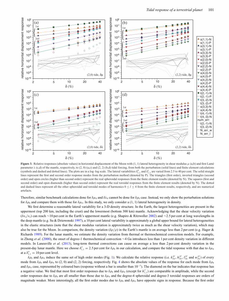
together against the perturbation solutions.Results are shown in Fig. 3 for four individual cases: (2, 0) and (2, 2) forcing on δμ0 (top panels) and δλ0 (bottom panels), respectively.

Again, all the first and the second order spheroidal and toroidal modes (triangles and squares in Fig. 3, respectively) predicted by theperturbation method are also the most significant modes from the finite element solutions, and the perturbation solutions (solid lines in Fig. 3)match the corresponding finite element solutions remarkably well (Fig. 3 and Table 1). Also, the horizontal displacement responses due toδμ0 are larger than those due to δλ0 by on average an order of magnitude (Figs 3a and b verse c and d), similar to what we find for radialdisplacement responses. The (relative) horizontal displacement responses (Fig. 3) are similar in amplitude to the radial displacement responses(Fig. 2 for δλ0 and fig. 2 of Qin et al. (2014) for δμ0). An exception is mode s1(1, 1) due to δμ0. The horizontal displacement response |l1′

1,1(a)|is one of the largest responses and is about two orders of magnitude larger than the corresponding radial displacement response |h1′

1,1(a)|[Figs 3a and b verse fig. 2 of Qin et al. (2014)].

For δμ0 cases, both (2, 0) and (2, 2) forces induce the same set of toroidal modes in the response, which are t1(2,−1) and t2(3, −2).The toroidal response |w1′

2,−1(a)| is surprisingly large, especially for that induced by (2, 0) forcing, and when δμ

1,1 is sufficiently large (e.g.δ

μ

1,1 ≥ 30 per cent), |w1′2,−1(a)| is even close to 1. The finite element solutions clearly show toroidal modes t3(4, −1) and t3(4, −3) (open

diamonds in Figs 3a and b). Although these two modes are predicted to exist at the third order of perturbation, their responses are at thesame level as those second order degree-4 responses. Note that δλ0 does not induce any toroidal modes, which is evident in Figs 3(c) and (d):|w1′

2,−1(a)| and |w2′3,−2(a)| are both at the noise level (dashed lines in corresponding colours).

4.2 Density anomaly effect on tidal response

We now explore the effect of lateral heterogeneity in density ρ on tidal response. Because including density anomaly δρ0 brings additional forcebalance terms into the governing equations, it is unclear how this complication can be implemented in our current finite element formulation.

Tidal response of a terrestrial planet 101

Figure 3. Relative responses (absolute values) in horizontal displacement of the Moon with (1, 1) lateral heterogeneity in shear modulus μ (a,b) and first Lameparameter λ (c,d) of the mantle, respectively, to (2, 0) (a,c) and (2, 2) (b,d) tidal forcing, from both the perturbation (solid lines) and finite element calculations(symbols and dashed and dotted lines). The plots are in a log–log scale. The lateral variabilities δ

μ

1,1 and δλ1,1 are varied from 2.5 to 40 per cent. The solid straight

lines represent the first and second order response modes from the perturbation method (denoted by P). The triangles (first order), inverted triangles (secondorder) and open circles (higher than second order) represent the real spheroidal responses from the finite element results (denoted by N). The squares (first andsecond order) and open diamonds (higher than second order) represent the real toroidal responses from the finite element results (denoted by N). The dottedand dashed lines represent all the other spheroidal and toroidal modes of harmonics 0 ≤ l ≤ 4 from the finite element results, respectively, and are numericalartefacts.

Therefore, similar benchmark calculations done for δμ0 and δλ0 cannot be done for δρ0 case. Instead, we only show the perturbation solutionsfor δρ0 and compare them with those for δμ0. In this study, we only consider a (1, 1) lateral heterogeneity in density.

We first determine a reasonable lateral variability for a 3-D density structure. In the Earth, the largest heterogeneities are present in theuppermost (top 200 km, including the crust) and the lowermost (bottom 300 km) mantle. Acknowledging that the shear velocity variation(δvs/vs) can reach ∼10 per cent in the Earth’s uppermost mantle (e.g. Shapiro & Ritzwoller 2002) and ∼2.5 per cent at long wavelengths inthe deep mantle (e.g. Su & Dziewonski 1997), a 10 per cent lateral variability is approximately a global upper bound for lateral heterogeneitiesin the elastic structures (note that the shear modulus variation is approximately twice as much as the shear velocity variation), which mayalso be true for the Moon. In comparison, the density variation (δρ/ρ) in the Earth’s mantle is on average less than 2 per cent (e.g. Hager &Richards 1989). For the lunar mantle, we estimate the density variation from thermal or thermochemical convection models. For example,in Zhong et al. (2000), the onset of degree-1 thermochemical convection ∼4 Ga introduces less than 1 per cent density variation in differentmodels. In Laneuville et al. (2013), long-term thermal convections can cause on average a less than 2 per cent density variation in thepresent-day lunar mantle. Here we choose δ

ρ

1,1 = 2.5 per cent for δρ0 in our calculation, and compare the tidal response with that due to δμ0

at a δμ

1,1 = 10 per cent level.δρ0 and δμ0 induce the same set of high order modes (Fig. 1). We calculate the relative response (i.e. k D′

lm , hD′lm , l D′

lm and wD′lm ) of every

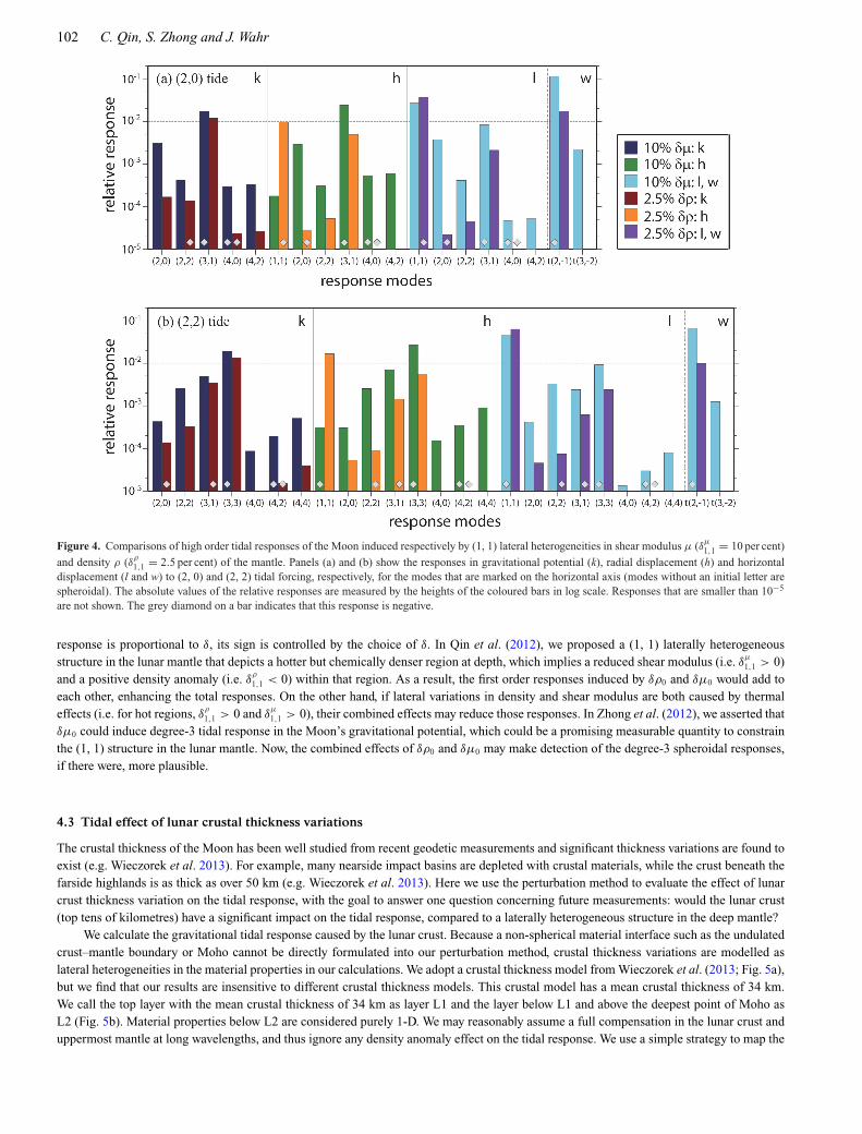
mode from δρ0 and δμ0 to (2, 0) and (2, 2) forcing, respectively. Fig. 4 shows the absolute values of the response for each mode from δρ0

and δμ0 case, represented by coloured bars (response without a bar is smaller than 10−5). The diamond on the bar indicates that response hasa negative value. We find that most first order responses due to δρ0 and δμ0 (except for h1′

1,1) are comparable in amplitude, while the secondorder responses due to δρ0 are all smaller than those due to δμ0 and the degree-4 spheroidal and degree-3 toroidal responses are orders ofmagnitude weaker. More interestingly, all the first order modes due to δρ0 and δμ0 have opposite signs in response. Because the first order

102 C. Qin, S. Zhong and J. Wahr

Figure 4. Comparisons of high order tidal responses of the Moon induced respectively by (1, 1) lateral heterogeneities in shear modulus μ (δμ

1,1 = 10 per cent)

and density ρ (δρ

1,1 = 2.5 per cent) of the mantle. Panels (a) and (b) show the responses in gravitational potential (k), radial displacement (h) and horizontaldisplacement (l and w) to (2, 0) and (2, 2) tidal forcing, respectively, for the modes that are marked on the horizontal axis (modes without an initial letter arespheroidal). The absolute values of the relative responses are measured by the heights of the coloured bars in log scale. Responses that are smaller than 10−5

are not shown. The grey diamond on a bar indicates that this response is negative.

response is proportional to δ, its sign is controlled by the choice of δ. In Qin et al. (2012), we proposed a (1, 1) laterally heterogeneousstructure in the lunar mantle that depicts a hotter but chemically denser region at depth, which implies a reduced shear modulus (i.e. δμ

1,1 > 0)and a positive density anomaly (i.e. δ

ρ

1,1 < 0) within that region. As a result, the first order responses induced by δρ0 and δμ0 would add toeach other, enhancing the total responses. On the other hand, if lateral variations in density and shear modulus are both caused by thermaleffects (i.e. for hot regions, δρ

1,1 > 0 and δμ

1,1 > 0), their combined effects may reduce those responses. In Zhong et al. (2012), we asserted thatδμ0 could induce degree-3 tidal response in the Moon’s gravitational potential, which could be a promising measurable quantity to constrainthe (1, 1) structure in the lunar mantle. Now, the combined effects of δρ0 and δμ0 may make detection of the degree-3 spheroidal responses,if there were, more plausible.

4.3 Tidal effect of lunar crustal thickness variations

The crustal thickness of the Moon has been well studied from recent geodetic measurements and significant thickness variations are found toexist (e.g. Wieczorek et al. 2013). For example, many nearside impact basins are depleted with crustal materials, while the crust beneath thefarside highlands is as thick as over 50 km (e.g. Wieczorek et al. 2013). Here we use the perturbation method to evaluate the effect of lunarcrust thickness variation on the tidal response, with the goal to answer one question concerning future measurements: would the lunar crust(top tens of kilometres) have a significant impact on the tidal response, compared to a laterally heterogeneous structure in the deep mantle?

We calculate the gravitational tidal response caused by the lunar crust. Because a non-spherical material interface such as the undulatedcrust–mantle boundary or Moho cannot be directly formulated into our perturbation method, crustal thickness variations are modelled aslateral heterogeneities in the material properties in our calculations. We adopt a crustal thickness model from Wieczorek et al. (2013; Fig. 5a),but we find that our results are insensitive to different crustal thickness models. This crustal model has a mean crustal thickness of 34 km.We call the top layer with the mean crustal thickness of 34 km as layer L1 and the layer below L1 and above the deepest point of Moho asL2 (Fig. 5b). Material properties below L2 are considered purely 1-D. We may reasonably assume a full compensation in the lunar crust anduppermost mantle at long wavelengths, and thus ignore any density anomaly effect on the tidal response. We use a simple strategy to map the

Tidal response of a terrestrial planet 103

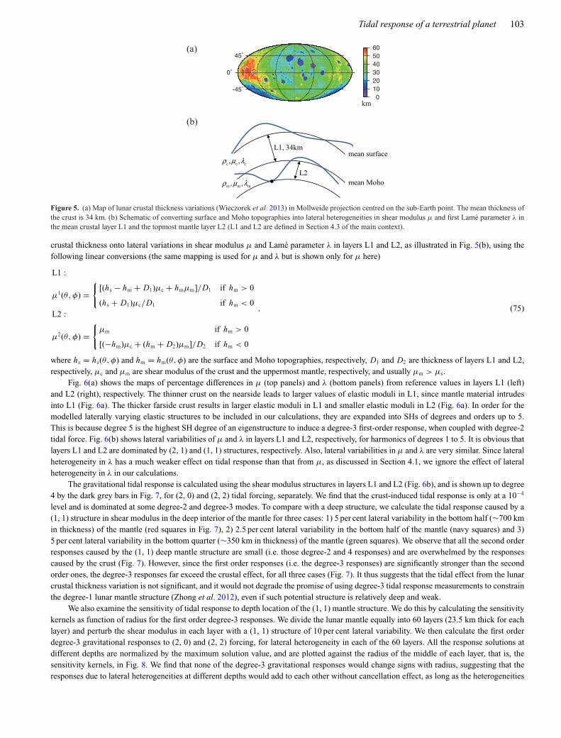
Figure 5. (a) Map of lunar crustal thickness variations (Wieczorek et al. 2013) in Mollweide projection centred on the sub-Earth point. The mean thickness ofthe crust is 34 km. (b) Schematic of converting surface and Moho topographies into lateral heterogeneities in shear modulus μ and first Lame parameter λ inthe mean crustal layer L1 and the topmost mantle layer L2 (L1 and L2 are defined in Section 4.3 of the main context).

crustal thickness onto lateral variations in shear modulus μ and Lame parameter λ in layers L1 and L2, as illustrated in Fig. 5(b), using thefollowing linear conversions (the same mapping is used for μ and λ but is shown only for μ here)

L1 :

μ1(θ, φ) ={

[(hs − hm + D1)μc + hmμm]/D1 if hm > 0

(hs + D1)μc/D1 if hm < 0L2 :

μ2(θ, φ) ={

μm if hm > 0

[(−hm)μc + (hm + D2)μm]/D2 if hm < 0

, (75)

where hs = hs(θ, φ) and hm = hm(θ, φ) are the surface and Moho topographies, respectively, D1 and D2 are thickness of layers L1 and L2,respectively, μc and μm are shear modulus of the crust and the uppermost mantle, respectively, and usually μm > μs.

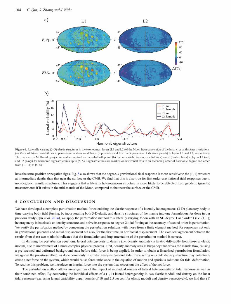
Fig. 6(a) shows the maps of percentage differences in μ (top panels) and λ (bottom panels) from reference values in layers L1 (left)and L2 (right), respectively. The thinner crust on the nearside leads to larger values of elastic moduli in L1, since mantle material intrudesinto L1 (Fig. 6a). The thicker farside crust results in larger elastic moduli in L1 and smaller elastic moduli in L2 (Fig. 6a). In order for themodelled laterally varying elastic structures to be included in our calculations, they are expanded into SHs of degrees and orders up to 5.This is because degree 5 is the highest SH degree of an eigenstructure to induce a degree-3 first-order response, when coupled with degree-2tidal force. Fig. 6(b) shows lateral variabilities of μ and λ in layers L1 and L2, respectively, for harmonics of degrees 1 to 5. It is obvious thatlayers L1 and L2 are dominated by (2, 1) and (1, 1) structures, respectively. Also, lateral variabilities in μ and λ are very similar. Since lateralheterogeneity in λ has a much weaker effect on tidal response than that from μ, as discussed in Section 4.1, we ignore the effect of lateralheterogeneity in λ in our calculations.

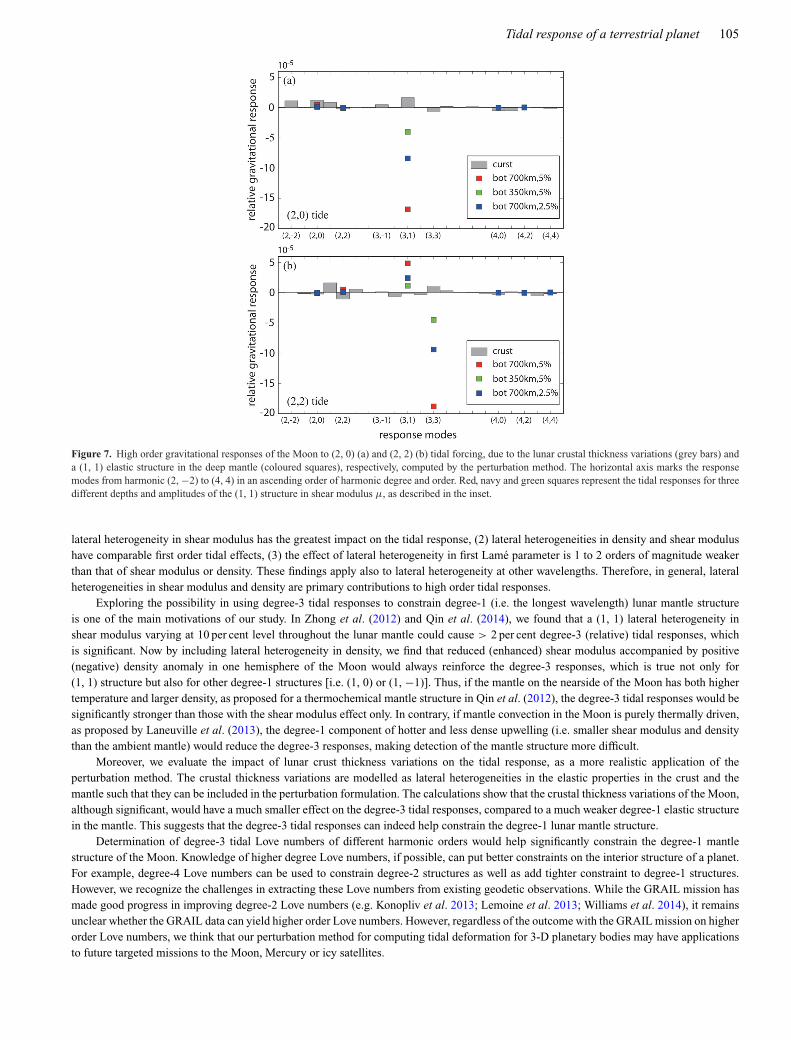
The gravitational tidal response is calculated using the shear modulus structures in layers L1 and L2 (Fig. 6b), and is shown up to degree4 by the dark grey bars in Fig. 7, for (2, 0) and (2, 2) tidal forcing, separately. We find that the crust-induced tidal response is only at a 10−4

level and is dominated at some degree-2 and degree-3 modes. To compare with a deep structure, we calculate the tidal response caused by a(1, 1) structure in shear modulus in the deep interior of the mantle for three cases: 1) 5 per cent lateral variability in the bottom half (∼700 kmin thickness) of the mantle (red squares in Fig. 7), 2) 2.5 per cent lateral variability in the bottom half of the mantle (navy squares) and 3)5 per cent lateral variability in the bottom quarter (∼350 km in thickness) of the mantle (green squares). We observe that all the second orderresponses caused by the (1, 1) deep mantle structure are small (i.e. those degree-2 and 4 responses) and are overwhelmed by the responsescaused by the crust (Fig. 7). However, since the first order responses (i.e. the degree-3 responses) are significantly stronger than the secondorder ones, the degree-3 responses far exceed the crustal effect, for all three cases (Fig. 7). It thus suggests that the tidal effect from the lunarcrustal thickness variation is not significant, and it would not degrade the promise of using degree-3 tidal response measurements to constrainthe degree-1 lunar mantle structure (Zhong et al. 2012), even if such potential structure is relatively deep and weak.

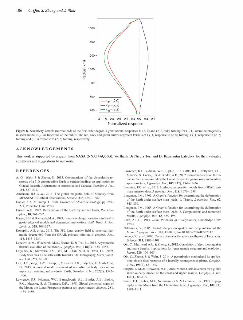
We also examine the sensitivity of tidal response to depth location of the (1, 1) mantle structure. We do this by calculating the sensitivitykernels as function of radius for the first order degree-3 responses. We divide the lunar mantle equally into 60 layers (23.5 km thick for eachlayer) and perturb the shear modulus in each layer with a (1, 1) structure of 10 per cent lateral variability. We then calculate the first orderdegree-3 gravitational responses to (2, 0) and (2, 2) forcing, for lateral heterogeneity in each of the 60 layers. All the response solutions atdifferent depths are normalized by the maximum solution value, and are plotted against the radius of the middle of each layer, that is, thesensitivity kernels, in Fig. 8. We find that none of the degree-3 gravitational responses would change signs with radius, suggesting that theresponses due to lateral heterogeneities at different depths would add to each other without cancellation effect, as long as the heterogeneities

104 C. Qin, S. Zhong and J. Wahr

Figure 6. Laterally varying (3-D) elastic structures in the two topmost layers (L1 and L2) of the Moon from conversion of the lunar crustal thickness variations.(a) Maps of lateral variabilities in percentage in shear modulus μ (top panels) and first Lame parameter λ (bottom panels) in layers L1 and L2, respectively.The maps are in Mollweide projection and are centred on the sub-Earth point. (b) Lateral variabilities in μ (solid lines) and λ (dashed lines) in layers L1 (red)and L2 (navy) for harmonic eigenstructures up to (5, 5). Eigenstructures are marked on horizontal axis in an ascending order of harmonic degree and order,from (1, −1) to (5, 5).

have the same positive or negative signs. Fig. 8 also shows that the degree-3 gravitational tidal response is more sensitive to the (1, 1) structureat intermediate depths than that near the surface or the CMB. We find that this is also true for first order gravitational tidal responses due tonon-degree-1 mantle structures. This suggests that a laterally heterogeneous structure is more likely to be detected from geodetic (gravity)measurements if it exists in the mid-mantle of the Moon, compared to that near the surface or the CMB.

5 C O N C LU S I O N A N D D I S C U S S I O N

We have developed a complete perturbation method for calculating the elastic response of a laterally heterogeneous (3-D) planetary body totime-varying body tidal forcing, by incorporating both 3-D elastic and density structures of the mantle into one formulation. As done in ourprevious study (Qin et al. 2014), we apply the perturbation method to a laterally varying Moon with an SH degree 1 and order 1 (i.e. (1, 1))heterogeneity in its elastic or density structure, and solve its response to degree-2 tidal forcing at the accuracy of second order in perturbation.We verify the perturbation method by comparing the perturbation solutions with those from a finite element method, for responses not onlyin gravitational potential and radial displacement but also, for the first time, in horizontal displacement. The excellent agreement between theresults from these two methods indicates that the formulation and implementation of the perturbation method is correct.

In deriving the perturbation equations, lateral heterogeneity in density (i.e. density anomaly) is treated differently from those in elasticmoduli, due to involvement of a more complex physical process. First, density anomaly acts as buoyancy that drives the mantle flow, causinga pre-stressed and deformed background state before tidal force is being applied. In order to obtain a linearized perturbation formulation,we ignore the pre-stress effect, as done commonly in similar analyses. Second, tidal force acting on a 3-D density structure may potentiallycause a net force on the system, which would cause force imbalance in the equation of motion and spurious solutions for tidal deformation.To resolve this problem, we introduce an inertial force into the system that zeroes out the effect of the net force.

The perturbation method allows investigations of the impact of individual sources of lateral heterogeneity on tidal response as well astheir combined effect. By comparing the individual effects of a (1, 1) lateral heterogeneity in two elastic moduli and density on the lunartidal response (e.g. using lateral variability upper bounds of 10 and 2.5 per cent for elastic moduli and density, respectively), we find that (1)

Tidal response of a terrestrial planet 105

Figure 7. High order gravitational responses of the Moon to (2, 0) (a) and (2, 2) (b) tidal forcing, due to the lunar crustal thickness variations (grey bars) anda (1, 1) elastic structure in the deep mantle (coloured squares), respectively, computed by the perturbation method. The horizontal axis marks the responsemodes from harmonic (2, −2) to (4, 4) in an ascending order of harmonic degree and order. Red, navy and green squares represent the tidal responses for threedifferent depths and amplitudes of the (1, 1) structure in shear modulus μ, as described in the inset.

lateral heterogeneity in shear modulus has the greatest impact on the tidal response, (2) lateral heterogeneities in density and shear modulushave comparable first order tidal effects, (3) the effect of lateral heterogeneity in first Lame parameter is 1 to 2 orders of magnitude weakerthan that of shear modulus or density. These findings apply also to lateral heterogeneity at other wavelengths. Therefore, in general, lateralheterogeneities in shear modulus and density are primary contributions to high order tidal responses.

Exploring the possibility in using degree-3 tidal responses to constrain degree-1 (i.e. the longest wavelength) lunar mantle structureis one of the main motivations of our study. In Zhong et al. (2012) and Qin et al. (2014), we found that a (1, 1) lateral heterogeneity inshear modulus varying at 10 per cent level throughout the lunar mantle could cause > 2 per cent degree-3 (relative) tidal responses, whichis significant. Now by including lateral heterogeneity in density, we find that reduced (enhanced) shear modulus accompanied by positive(negative) density anomaly in one hemisphere of the Moon would always reinforce the degree-3 responses, which is true not only for(1, 1) structure but also for other degree-1 structures [i.e. (1, 0) or (1, −1)]. Thus, if the mantle on the nearside of the Moon has both highertemperature and larger density, as proposed for a thermochemical mantle structure in Qin et al. (2012), the degree-3 tidal responses would besignificantly stronger than those with the shear modulus effect only. In contrary, if mantle convection in the Moon is purely thermally driven,as proposed by Laneuville et al. (2013), the degree-1 component of hotter and less dense upwelling (i.e. smaller shear modulus and densitythan the ambient mantle) would reduce the degree-3 responses, making detection of the mantle structure more difficult.

Moreover, we evaluate the impact of lunar crust thickness variations on the tidal response, as a more realistic application of theperturbation method. The crustal thickness variations are modelled as lateral heterogeneities in the elastic properties in the crust and themantle such that they can be included in the perturbation formulation. The calculations show that the crustal thickness variations of the Moon,although significant, would have a much smaller effect on the degree-3 tidal responses, compared to a much weaker degree-1 elastic structurein the mantle. This suggests that the degree-3 tidal responses can indeed help constrain the degree-1 lunar mantle structure.

Determination of degree-3 tidal Love numbers of different harmonic orders would help significantly constrain the degree-1 mantlestructure of the Moon. Knowledge of higher degree Love numbers, if possible, can put better constraints on the interior structure of a planet.For example, degree-4 Love numbers can be used to constrain degree-2 structures as well as add tighter constraint to degree-1 structures.However, we recognize the challenges in extracting these Love numbers from existing geodetic observations. While the GRAIL mission hasmade good progress in improving degree-2 Love numbers (e.g. Konopliv et al. 2013; Lemoine et al. 2013; Williams et al. 2014), it remainsunclear whether the GRAIL data can yield higher order Love numbers. However, regardless of the outcome with the GRAIL mission on higherorder Love numbers, we think that our perturbation method for computing tidal deformation for 3-D planetary bodies may have applicationsto future targeted missions to the Moon, Mercury or icy satellites.

106 C. Qin, S. Zhong and J. Wahr

Figure 8. Sensitivity kernels (normalized) of the first order degree-3 gravitational responses to (2, 0) and (2, 2) tidal forcing for (1, 1) lateral heterogeneityin shear modulus μ, as functions of the radius. The red, navy and green curves represent kernels of (3, 1) response to (2, 0) forcing, (3, 1) response to (2, 2)forcing and (3, 3) response to (2, 2) forcing, respectively.

A C K N OW L E D G E M E N T S

This work is supported by a grant from NASA (NNX14AQ06G). We thank Dr Nicola Tosi and Dr Konstantin Latychev for their valuablecomments and suggestions to our work.

R E F E R E N C E S

A, G., Wahr, J. & Zhong, S., 2013. Computations of the viscoelastic re-sponse of a 3-D compressible Earth to surface loading: an application toGlacial Isostatic Adjustment in Antarctica and Canada, Geophys. J. Int.,192, 557–572.

Anderson, B.J. et al., 2011. The global magnetic field of Mercury fromMESSENGER orbital observations, Science, 333, 1859–1862.

Dahlen, F.A. & Tromp, J., 1998. Theoretical Global Seismology, pp. 268–271, Princeton Univ. Press.

Farrell, W.E., 1972. Deformation of the Earth by surface loads, Rev. Geo-phys., 10, 761–797.

Hager, B.H. & Richards, M.A., 1989. Long-wavelength variations in Earth’sgeoid: physical models and dynamical implications, Phil. Trans. R. Soc.Lond., A, 328, 309–327.

Konopliv, A.S. et al., 2013. The JPL lunar gravity field to spherical har-monic degree 660 from the GRAIL primary mission, J. geophys. Res.,118, 1415–1434.

Laneuville, M., Wieczorek, M.A., Breuer, D. & Tosi, N., 2013. Asymmetricthermal evolution of the Moon, J. geophys. Res., 118(7), 1435–1452.

Latychev, K., Mitrovica, J.X., Ishii, M., Chan, N.-H. & Davis, J.L., 2009.Body tides on a 3-D elastic earth: toward a tidal tomography, Earth planet.Sci. Lett., 277, 86–90.

Lau, H.C., Yang, H.-Y., Tromp, J., Mitrovica, J.X., Latychev, K. & Al-Attar,D., 2015. A normal mode treatment of semi-diurnal body tides on anaspherical, rotating and anelastic Earth, Geophys. J. Int., 202(2), 1392–1406.

Lawrence, D.J., Feldman, W.C., Barraclough, B.L., Binder, A.B., Elphic,R.C., Maurice, S. & Thomsen, D.R., 1998. Global elemental maps ofthe Moon: the Lunar Prospector gamma-ray spectrometer, Science, 281,1484–1489.

Lawrence, D.J., Feldman, W.C., Elphic, R.C., Little, R.C., Prettyman, T.H.,Maurice, S., Lucey, P.G. & Binder, A.B., 2002. Iron abundances on the lu-nar surface as measured by the Lunar Prospector gamma-ray and neutronspectrometers, J. geophys. Res., 107(E12), 13-1–13-26.

Lemoine, F.G. et al., 2013. High-degree gravity models from GRAIL pri-mary mission data, J. geophys. Res., 118, 1676–1698.

Longman, I.M., 1962. A Green’s function for determining the deformationof the Earth under surface mass loads: 1. Theory, J. geophys. Res., 67,845–850.

Longman, I.M., 1963. A Green’s function for determining the deformationof the Earth under surface mass loads: 2. Computations and numericalresults, J. geophys. Res., 68, 485–496.

Love, A.E.H., 1911. Some Problems of Geodynamics, Cambridge Univ.Press.

Nakamura, Y., 2005. Farside deep moonquakes and deep interior of theMoon, J. geophys. Res., 110, E01001, doi:10.1029/2004JE002332.

Porco, C.C. et al., 2006. Cassini observes the active south pole of Enceladus,Science, 311, 1393–1401.

Qin, C., Muirhead, A.C. & Zhong, S., 2012. Correlation of deep moonquakesand mare basalts: implications for lunar mantle structure and evolution,Icarus, 220, 100–105.

Qin, C., Zhong, S. & Wahr, J., 2014. A perturbation method and its applica-tion: elastic tidal response of a laterally heterogeneous planet, Geophys.J. Int., 199(2), 631–647.

Shapiro, N.M. & Ritzwoller, M.H., 2002. Monte-Carlo inversion for a globalshear-velocity model of the crust and upper mantle, Geophys. J. Int.,151(1), 88–105.

Smith, D.E., Zuber, M.T., Neumann, G.A. & Lemoine, F.G., 1997. Topog-raphy of the Moon from the Clementine lidar, J. geophys. Res., 102(E1),1591–1611.

Tidal response of a terrestrial planet 107

Smith, D.E. et al., 2010. The lunar orbiter laser altimeter investigation onthe lunar reconnaissance orbiter mission, Space Sci. Rev., 150, 209–241.

Spencer, J.R. et al., 2006. Cassini encounters Enceladus: background andthe discovery of a south polar hot spot, Science, 311, 1401–1405.

Su, W. & Dziewonski, A.M., 1997. Simultaneous inversion for 3-D varia-tions in shear and bulk velocity in the mantle, Phys. Earth planet. Inter.,100, 135–156.

Tapley, B.D., Bettadpur, S., Watkins, M. & Reigber, C., 2004. The grav-ity recovery and climate experiment: mission overview and early results,Geophys. Res. Lett., 31(9), doi:10.1029/2004GL019920.

Tompkins, S. & Pieters, C.M., 1999. Mineralogy of the lunar crust: resultsfrom Clementine, Meteorit. Planet. Sci., 34, 25–41.

Tromp, J. & Mitrovica, J.X., 1999a. Surface loading of a viscoelastic earth–I.General theory, Geophys. J. Int., 137, 847–855.

Tromp, J. & Mitrovica, J.X., 1999b. Surface loading of a viscoelastic earth–II. Spherical models, Geophys. J. Int., 137, 856–872.

Wahr, J., Selvans, Z.A., Mullen, M.E., Barr, A.C., Collins, G.C., Selvans,M.M. & Pappalardo, R.T., 2009. Modeling stresses on satellites due tononsynchronous rotation and orbital eccentricity using gravitational po-tential theory, Icarus, 200, 188–206.

Weber, R.C., Lin, P.Y., Garnero, E.J., Williams, Q. & Lognonne, P., 2011.Seismic detection of the lunar core, Science, 331, 309–312.

Wieczorek, M.A. et al., 2006. The constitution and structure of the lunarinterior, Rev. Mineral. Geochem., 60, 221–364.

Wieczorek, M.A. et al., 2013. The crust of the Moon as seen by GRAIL,Science, 339, 671–675.

Williams, J.G. et al., 2014. Lunar interior properties from the GRAIL mis-sion, J. geophys. Res., 119, 1546–1578.

Zhong, S., Parmentier, E.M. & Zuber, M.T., 2000. A dynamic origin for theglobal asymmetry of lunar mare basalts, Earth planet. Sci. Lett., 177(3),131–140.

Zhong, S., Paulson, A. & Wahr, J., 2003. Three-dimensional finite-elementmodelling of Earth’s viscoelastic deformation: effects of lateral variationsin lithospheric thickness, Geophys. J. Int., 155, 679–695.

Zhong, S., Qin, C., A, G. & Wahr, J., 2012. Can tidal tomography be usedto unravel the long-wavelength structure of the lunar interior?, Geophys.Res. Lett., 39, L15201, doi:10.1029/2012GL052362.

Zuber, M.T., 2001. The crust and mantle of Mars, Nature, 412, 220–227.Zuber, M.T., Smith, D.E., Lemoine, F.G. & Neumann, G.A., 1994. The shape

and internal structure of the Moon from the Clementine mission, Science,266, 1839–1843.

Zuber, M.T. et al., 2013. Gravity field of the Moon from the Grav-ity Recovery and Interior Laboratory (GRAIL) mission, Science, 339,668–671.

A P P E N D I X A : H A R M O N I C E X PA N S I O N O F M O D E C O U P L I N G T E R M S

The termsFD ,BD , GD andHD , which involve mode coupling between the lateral heterogeneities in material properties and the lower order(D − 1) response, exist only in the first and the second order perturbation equations. In order to implement the propagator matrix solutionmethod, we expand those coupling terms into different harmonics that separate into either spheroidal (s) or toroidal (t) mode. Here, we callthe lower order response or mode as ‘parent’ and the modes that result from the coupling as ‘child’. A ‘child’ at a specific mode is indicatedby a non-trivial set of expansion coefficients of the coupling terms at that harmonic [eq. (A11) in Qin et al. (2014) for VSH expansion].Assuming that the ‘parent’, a single eigenstructure of the lateral heterogeneities, and a ‘child’ are at harmonics (l0, m0), (l1, m1) and (l, m),respectively, expansion of the coupling terms can be generalized into four categories, depending on whether it is spheroidal or toroidal thatthe ‘parent’ and the ‘child’ belong to.

Following eqs (49) and (51), we divide F x,Dlm and Bx,D

lm further into δμ0, δλ0 and δρ0 induced terms, as

F x,Dlm = F x,D

μ,lm + F x,Dλ,lm + F x,D

ρ,lm (A1)

and

Bx,Dlm = Bx,D

μ,lm + Bx,Dλ,lm, (A2)

where x denotes p, b or c component (corresponding to VSH basis functions in eq. (38)). Note that a spheroidal (toroidal) mode does nothave c (p or b) component(s). The four categories of expansion coefficients ofFD ,BD , GD andHD are thus expressed, respectively, as

I) s(l0, m0) ⊗ (l1, m1) → s(l, m)i. δμ0 induced:

F p,Dμ,lm =

μ

l1m1μ0

[a1

(U + 2U

r− 2U

r 2

)+ a2

V

r 2+ a3

S

μ0r

]D−1

l0m0

, (A3)

Fb,Dμ,lm =

μ

l1m1μ0

[a4

(S

μ0+ 3S

μ0r

)+ a5

U

r 2+ a6

V

r 2

]D−1

l0m0

, (A4)

B p,Dμ,lm =

μ

l1m1μ0

[a1U

]D−1

l0m0, (A5)

Bb,Dμ,lm =

μ

l1m1[a4 S]D−1

l0m0, (A6)

where []D−1l0m0

means the enclosed r-dependent quantities belong to mode (l0, m0) at the order of perturbation D − 1.

ii. δλ0 induced:

F p,Dλ,lm = λ

l1m1λ0

[b1 X

]D−1

l0m0, (A7)

108 C. Qin, S. Zhong and J. Wahr

Fb,Dλ,lm = λ

l1m1λ0

[b2

X

r

]D−1

l0m0

, (A8)

B p,Dλ,lm = λ

l1m1λ0 [b1 X ]D−1

l0m0, (A9)

Bb,Dλ,lm = 0, (A10)

where X D−1l0m0

= [U + 2Ur − l0(l0+1)V

r ]D−1l0m0

.

iii. δρ0 induced:

F p,Dρ,lm =

ρ

l1m1ρ0

[c1(g0 X − K ) + c2g0

V

r

]D−1

l0m0

+ f p,Dρ,lm, (A11)

Fb,Dρ,lm = −

ρ

l1m1ρ0

[c3

K

r

]D−1

l0m0

+ f b,Dρ,lm, (A12)

where f p,Dρ,lm and f b,D

ρ,lm are from the additional terms that depend on the order of perturbation D [eqs (26) and (27)]. When D = 1 ,

f p,1ρ,lm = −

ρ

l1m1ρ0c1�

tdltd,mtd

− δ(l − 1, m − m ′)ρ0f0

M, (A13)

f b,1ρ,lm = −

ρ

l1m1ρ0c3

�tdltd,mtd

r− δ(l − 1, m − m ′)ρ0

f0

M, (A14)

where we assume the tidal potential is at harmonic (ltd, m td) and thus Vtd = �tdltd,mtd

Yltd,mtd . Here, δ(x, y) = 1 if and only if x = y = 0 ,otherwise δ(x, y) = 0. Therefore, the second terms on the right-hand side of (A13) and (A14) are non-vanishing only when the forcing term−δρ0∇Vtd causes a degree-1 net force at (1, m ′) [see eq. (11) for the definition of f0

M ]. When D = 2 ,

f p,2ρ,lm = −

ρ

l1m1ρ0

{δ(l − l ′′, m − m ′′)c1

f0

M

}, (A15)

f b,2ρ,lm = −

ρ

l1m1ρ0

{δ(l − l ′′, m − m ′′)c3

f0

M

}, (A16)

where (l ′′, m ′′) is the mode allowed from the coupling of (1, m ′) and (l1, m1) [eq. (27)]. In addition, GD andHD are caused by δρ0 only,where

G Dlm =

ρ

l1m1ρ0

[c1 X + c2

V

r

]D−1

l0m0

(A17)

and

H Dlm =

ρ

l1m1ρ0 [c1U ]D−1

l0m0, (A18)

respectively. The constants a1, a2, . . . , a6, b1, b2, c1, c2 and c3 are coupling constants and they vary for different couplings.

II) s(l0, m0) ⊗ (l1, m1) → t(l, m)i. δμ0 induced:

Fc,Dμ,lm =

μ

l1m1μ0

[a1

(S

μ0+ 3S

μ0r

)+ a2

V

r 2

]D−1

l0m0

, (A19)

Bc,Dμ,lm =

μ

l1m1[a1 S]D−1

l0m0. (A20)

ii. δλ0 does not induce toroidal mode, therefore Fc,Dλ,lm = Bc,D

λ,lm = 0.iii. δρ0 induced:

Fc,Dρ,lm = −

ρ

l1m1ρ0

[c1

K

r

]D−1

l0m0

+ f c,Dρ,lm, (A21)

Tidal response of a terrestrial planet 109

where when D = 1

f c,1ρ,lm = −

ρ

l1m1ρ0c1

�tdL ,M

r, (A22)

when D = 2

f c,2ρ,lm = −

ρ

l1m1ρ0

{δ(l − l ′′, m − m ′′)c1

f0

M

}. (A23)

Note that GD or HD does not appear in the toroidal equations. The coupling constants a1, a2, a3 and c1 are different from those in thefirst category.

III) t(l0, m0) ⊗ (l1, m1) → s(l, m)i. δμ0 induced:

F p,Dμ,lm =

μ

l1m1μ0

[a1

T

μ0r

]D−1

l0m0

, (A24)

Fb,Dμ,lm =

μ

l1m1μ0

[a2

(T

μ0+ 3T

μ0r

)+ a3

W

r 2

]D−1

l0m0

, (A25)

B p,Dμ,lm = 0, (A26)

Bb,Dμ,lm =

μ

l1m1[a2T ]D−1

l0m0. (A27)

ii. δρ0 induced:

F p,Dρ,lm =

ρ

l1m1ρ0g0

[c1

W

r

]D−1

l0m0

, (A28)

Fb,Dρ,lm = 0. (A29)

Note that (A28) and (A29) do not contain extra terms f p,Dρ,lm or f b,D

ρ,lm .

G Dlm =

ρ

l1m1ρ0

[c1

W

r

]D−1

l0m0

, (A30)

H Dlm = 0. (A31)

A toroidal mode will not couple with δλ0 to induce a ‘child’ mode.

IV) t(l0, m0) ⊗ (l1, m1) → t(l, m)i. δμ0 induced:

Fc,Dμ,lm =

μ

l1m1μ0

[a1

(T

μ0+ 3T

μ0r

)+ a2

W

r 2

]D−1

l0m0

, (A32)

Bc,Dμ,lm =

μ

l1m1[a1T ]D−1

l0m0. (A33)

We find that a toroidal mode coupling with δρ0 does not further induce any toroidal mode, meaning Fc,Dρ,lm = G D

lm = H Dlm = 0.

A P P E N D I X B : S O LU T I O N P RO C E D U R E O F P E RT U R B AT I O N M E T H O D

The whole solution procedure of the perturbation method is coded up and can be summarized by a flowchart in Fig. B1. At the initial step,the mode of tidal forcing [i.e. (l0, m0)], the 1-D reference properties of the planet and the 3-D elastic and density structures (i.e. lateralheterogeneities in eigenstructures, see eqs 39–41) are set up. All quantities are non-dimensionalized. Then, an outer loop solves the modecouplings up to the second order of perturbation for each eigenstructure in the lateral heterogeneities. All the high order response modes andtheir associated matrix equations are determined, depending on different ‘parent’–‘child’ pairings (see Appendix A). An inner loop then goesthrough all the response modes and solves for the tidal responses correspondingly, mode by mode, from zeroth to second order of perturbation.The propagator matrix method based on a fourth-order Runge–Kutta numerical scheme is used to solve the matrix equations [appendix C inQin et al. (2014)]. The total tidal response is thus the sum of responses of each mode.

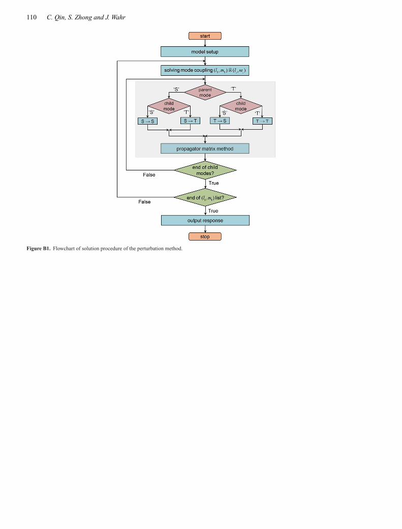
110 C. Qin, S. Zhong and J. Wahr

Figure B1. Flowchart of solution procedure of the perturbation method.