Early Research Directions: Geometric Analysis I & II

Geometry of Surfaces

Andrejs Treibergs

University of Utah

Friday, January 29, 2010

2. References

Notes on two lectures on geometric analysis.

1 “Geometry of Surfaces” given January 22, 2010,

2 “Intrinsic Geometry” given January 29, 2010.

The URL for these Beamer Slides: “Geometry of Surfaces”

http://www.math.utah.edu/~treiberg/GeomSurfSlides.pdf

3. Outline.

Surfaces of Euclidean Space and Riemannian Surfaces

Induced Metric

Hyperbolic Space.

Parabolicity.

Complete Manifolds with Finite Total Curvature.

4. Examples of Surfaces.

Some examples of what should be surfaces.

Graphs of functionsG2 = (x , y , z) ∈ R3 : z = f (x , y) and (x , y) ∈ U

where U ⊂ R2 is an open set.

Level sets, e.g.,S2 = (x , y , z) ∈ R3 : x2 + y2 + z2 = 1

This is the standard unit sphere.

Parameterized Surfaces, e.g.,

T2 =(

(A + a cosφ) cos θ, (A + a cosφ) sin θ, a sinφ))

: θ, φ ∈ R

is the torus with radii A > a > 0 constructed as a surface ofrevolution about the z-axis.

5. Local Coordinates.

A surface can locally be given by a curvilinear coordinate chart, alsocalled a parameterization. Let U ⊂ R2 be open. Let

X : U → R3

be a C1 function. Then we want M = X (U) to be a surface. At eachpoint P ∈ X (U) we can identify tangent vectors to the surface. IfP = X (a) some a ∈ U, then

Xi (a) =∂X

∂ui(a)

for i = 1, 2 are vectors in R3 tangent to the coordinate curves. To avoidsingularities at P, we shall assume that all X1(P)and X2(P) are linearlyindependent vectors. Then the tangent plane to the surface at P is

TPM = spanX1(P),X2(P).

6. Example of Local Coordinates.

For the graph G2 = (x , y , z) ∈ R3 : z = f (x , y) and (x , y) ∈ U onecoordinate chart covers the whole surface, X : U → G2 ∩ V = G2, where

X (u1, u2) = (u1, u2, f (u1, u2)).

where V = (u1, u2, u3) : (u1, u2) ∈ U and u3 ∈ R.The tangent vectors are thus

X1(u1, u2) =

(1, 0,

∂f

∂u1(u1, u2)

),

X2(u1, u2) =

(0, 1,

∂f

∂u2(u1, u2)

) (1)

which are linearly independent for every (u1, u2) ∈ U.

7. Definition of a Surface.

Definition

A connected subset M ⊂ R3 is a regular surface if to each P ∈ M, thereis an open neighborhood P ∈ V ⊂ R2, and a map

X : U → V ∩M

of an open set U ⊂ R2 onto V ∩M such that

1 X is differentiable. (In fact, we shall assume X is smooth (C∞)

2 X is a homeomorphism (X is continuous and has a continuousinverse)

3 The tangent vectors X1(a) and X2(a) are linearly independent for alla ∈ U.

8. Transition Functions.

Figure: Extrinsic: Coordinate Charts for Surface in E3

Suppose S ⊂ R3 is a surface and at P ∈ S there are two coordinatecharts σ : U → S and σ : U → S such that U and U are open subsets ofR2 and P ∈ σ(U) ∩ σ(U). Then on the overlap, for u ∈ σ−1(σ(U)), wehave the transition function

u = g(u) = σ−1(σ(u))which gives the change of coordinates map. These maps are smoothdiffeomorphisms on overlaps, by the Inverse Function Theorem.

9. Abstract Differentiable Manifold.

To abstract the idea of a regular surface, we drop the requirement thatM ⊂ R3 and just require that there is a topological space M that has acollection of coordinate charts, an atlas, whose transition functions aresmooth and consistently defined. Such an abstract surface is called adifferentiable manifold and the atlas of charts with correspondingtransition functions is called a differential structure.

Question: Are there differentiable manifolds that do not arise assubmanifolds of Euclidean space with the induced differential structure?Answer: No. (Provided we allow big codimension.)

Theorem (Whitney’s Embedding Theorem.)

Let Mn be an abstract, smooth differentiable manifold of dimension n.Then Mn is diffeomorphic to some W n ⊂ RN , an embedded regularsubmanifold provided N ≥ 2n + 1.

10. Lengths of Curves.

The Euclidean structure of R3, the usual dot product, gives a way tomeasure lengths and angles of vectors. If V = (v1, v2, v3) then its length

|V | =√

v21 + v2

2 + v23 =

√V • V

If W = (w1,w2,w3) then the angle α = ∠(V ,W ) is given by

cosα =V •W

|V | |W |.

If γ : [a, b] → M ⊂ R3 is a continuously differentiable curve, its length is

L(γ) =

∫ b

a|γ(t)| dt.

11. Induced Riemannian Metric.

If the curve is confined to a coordinate patch γ([a, b]) ⊂ X (U) ⊂ M,then we may factor through the coordinate chart. There are continuouslydifferentiable u(t) = (u1(t), u2(t)) ∈ U so that

γ(t) = X (u1(t), u2(t)) for all t ∈ [a, b].

Then the tangent vector may be written

γ(t) = X1(u1(t), u2(t)) u1(t) + X2(u1(t), u2(t)) u2(t)

so its length is

|γ|2 = X1 • X1 u21 + 2X1 • X2 u1u2 + X2 • X2 u2

2

For i , j = 1, 2 the Riemannian Metric is is given by the matrix function

gij(u) = Xi (u) • Xj(u)

Evidently, gij(u) is a smoothly varying, symmetric and positive definite.

12. Induced Riemannian Metric. -

Thus |γ(t)|2 =2∑

i=1

2∑j=1

gij(u(t)) ui (t) uj(t).

The length of the curve on the surface is determined by its velocity in thecoordinate patch u(t) and the metric gij(u).A vector field on the surface is also determined by functions in U usingthe basis. Thus if V and W are tangent vector fields, they may bewritten

V (u) = v1(u)X1(u)+v2(u)X2(u), W (u) = w1(u)X1(u)+w2(u)X2(u)

The R3 dot product can also be expressed by the metric. Thus

V •W = 〈V ,W 〉 =2∑

i ,j=1

gij v i w j .

where 〈·, ·〉 is an inner product on TpM that varies smoothly on M. ThisRiemannian metric is also called the First Fundamental Form.

13. Angle and Area via the Riemannian Metric.

If V and W are nonvanishing vector fields on M then their angleα = ∠(V ,W ) satisfies

cosα =〈V ,W 〉|V | |V |

which depends on coordinates of the vector fields and the metric.If D ⊂ U is a piecewise smooth subdomain in the patch, the area ifX (D) ⊂ M is also determined by the metric

A(X (D)) =

∫D|X1 × X2| du1 du2 =

∫D

√det(gij(u)) du1 du2

since if β = ∠(X1,X2) then

|X1 × X2|2 = sin2 β |X1|2 |X2|2 = (1− cos2 β) |X1|2 |X2|2

= |X1|2 |X2|2 − (X1 • X2)2 = g11g22 − g2

12.

14. Example in Local Coordinates. -

For the graph G2 = (x , y , z) ∈ R3 : z = f (x , y) and (x , y) ∈ U takethe patch X (u1, u2) = (u1, u2, f (u1, u2)).The metric components are gij = Xi • Xj so using (1),(

g11 g12

g21 g22

)=

(1 + f 2

1 f1f2f1f2 1 + f 2

2

)

where fi =∂f

∂ui. Thus gives the usual formula for area

det(gij) = 1 + f 21 + f 2

2

so

A(X (D)) =

∫D

√1 + f 2

1 + f 22 du1 du2.

15. Abstract Riemannian Manifold.

If we endow an abstract differentiable manifold Mn with a RiemannianMetric, a smoothly varying inner product on each tangent space that isconsistently defined on overlapping coordinate patches, the resultingobject is a Riemannian Manifold.

Question: Are there Riemannian manifolds that do not arise assubmanifolds of Euclidean space with the induced differential structureand Riemannian metric?Answer: No. (Provided we allow big codimension.)

Theorem (Nash’s Isometric Immersion Theorem.)

Let Mn be an abstract, smooth Riemannian manifold of dimension n.Then Mn is isometric to a smooth immersed submanifold W n ⊂ RN withinduced Riemannian metric provided that N ≥ n2 + 10n + 3.

John Nash had to invent some heavy duty PDE’s (the Nash ImplicitFunction Theorem) to solve Xi • Xj = gij for X .

16. Tensorial Nature of the Metric.

What is obvious when we think of a regular surface M ⊂ R3 is thatregardless of what coordinate system we use in the neighborhood ofP ∈ M, the inner product between two vectors, or the area of a domainor the length of the curve is the same because they are expressions of theEuclidean values. e.g., if we compute vectors and metrics in the U or theU coordinate systems near P,

2∑i ,j=1

gij(u) v i (u) w j(u) = V •W =2∑

i ,j=1

gij(u) v i (u) w j(u).

where points u = u(u) correspond under the transition function.

This also holds true in an abstract Riemanniam manifold. That isbecause the vector fields and the first fundamental form are tensors.Their transformations under change of coordinates exactly compensate tokeep geometric quantities invariant under change of coordinate.

17. Intrinsic Geometry.

Geometric quantities determined by the metric are called intrinsic. Adiffeomorphism between two abstract Riemanniam manifolds is called anisometry if it preserves lengths of curves, hence all intrinsic quantities.Equivalently, the Riemannian metrics are preserved. Thus if

f : (Mn, g) → (Mn, g)

is an isometry, then f : Mn → Mn is a diffeomorphism and f ∗g = gwhich means that for every vector fields V ,W on M and at every pointP ∈ M,

g(V (u),W (u))u = g(dfu(V (u)), dfu(V (u)))u

where dfu : TX (u) → TuM is the differential, u = u(u) correspond underthe transition map and where we have written the first fundamental formg(V ,W ).

WARNING: funtional analysts and geometric group theorists define“isometry” in a slightly different way.

18. Extrinsic Geometry.

Extrinsic Geometry deals with how M sits in its ambient space.

How to measure the shape of a regular surface M ⊂ R3? Suppose thate1 and e2 are orthonormal tangent vectors at P ∈ M and e3 is a unitvector perpendicular to TPM. Then near P, the surface may beparameterized as the graph over its tangent plane, where f (u1, u2) is the“height” above the tangent plane

X (u1, u2) = P + u1e1 + u2e2 + f (u1, u2)e3. (2)

So f (0) = 0 and Df (0) = 0. The Hessian of f at 0 gives the shapeoperator at P. It is also called the Second Fundamental Form.

hij(P) =∂2 f

∂ui ∂uj(0)

The Mean Curvature and Gaussian Curvature at P are

H(P) =1

2tr(hij(P)), K (P) = det(hij(P)).

19. Sphere Example.

The sphere about zero of radius r > 0 is an example

S2r = (x , y , z) ∈ R3 : x2 + y2 + z2 = r2.

Let P = (0, 0,−r) be the south pole. By a rotation (an isometry of R3),any point of S2

r can be moved to P with the surface coinciding. Thus thecomputation of H(P) and K (P) will be the same at all points of S2

r . Ife1 = (1, 0, 0), e2 = (0, 1, 0) and e3 = (0, 0, 1), the height function of (2)near zero is given by

f (u1, u2) = r −√

r2 − u21 − u2

2 .

The Hessian is

∂2f

∂ui uj(u) =

r2−u2

2

(r2−u21−u2

2)3/2

−u1u2

(r2−u21−u2

2)3/2

−u1u2u22

(r2−u21−u2

2)3/2

r2−u21

(r2−u21−u2

2)3/2

Thus the second fundamental form at P is

hij(P) = fij(0) =

(1r 00 1

r

)so H(P) =

1

rand K (P) =

1

r2

20. Graph Example.

If X (u1, u2) = (u1, u2, f (u1, u2)), by correcting for the slope at differentpoints one finds for all (u1, u2) ∈ U,

H(u1, u2) =

(1 + f 2

2

)f11 − 2f1 f2 f12 +

(1 + f 2

1

)f22

2(1 + f 2

1 + f 22

)3/2,

K (u1, u2) =f11 f22 − f 2

12(1 + f 2

1 + f 22

)2 .

21. The Plane and Cylinder are Isometric.

One imagines that one can roll up a piece of paper in R3 withoutchanging lengths of curves in the surface. Thus the plane and thecylinder are locally isometric. Let us check by computing the Riemannianmetrics at corresponding points. For any (u1, u2) ∈ R2 the plane isparameterized by

X (u1, u2) = (u1, u2, 0)so X1 = (1, 0, 0), X2 = (0, 1, 0) and so for the plane

gij =

(X1 • X1 X1 • X2

X2 • X1 X2 • X2

)=

(1 00 1

).

The cylinder Z2 = (x , y , z) : y2 + z2 = 1 may be parameterized byZ (u1, u2) = (u1, cos u2, sin u2). so Z1 = (1, 0, 0),

Z2 = (0,− sin u2, cos u2) and so for the cylinder

gij =

(Z1 • Z1 Z1 • Z2

Z2 • Z1 Z2 • Z2

)=

(1 00 1

).

The map f : X (u1, u2) 7→ Y (u1, u2) is an isometry because the metricsagree: f preserves lengths of curves.

22. Caps of Spheres are Not Rigid.

By manipulating half of a rubber ball that has been cut through itsequator, one sees that the cap can be deformed into a football shapewithout distorting intrinsic lengths of curves and angles of vectors. Thespherical cap is deformable through isometries: it is not rigid. (Rigidmeans that any isometry has to be a rigid motion of R3: composed ofrotations, translations or reflections.)

It turns out by Herglotz’s Theorem, all C3 closed K > 0 surfaces (hencesurfaces of convex bodies which are simply connected) are rigid.

23. Gauss’s Excellent Theorem.

So far, the formula for the Gauss Curvature has been given in terms ofthe second fundamental form and thus may depend on the extrinsicgeometry of the surface. However, Gauss discovered a formula that hedeemed excellent:

Theorem (Gauss’s Theorema Egregium 1828)

Let M2 ⊂ R3 be a smooth regular surface. Then the Gauss Curvaturemay be computed intrinsically from the metric and its first and secondderivatives.

In other words, the Gauss Curvature coincides at corresponding points ofisometric surfaces.

Thus the Gauss Curvature is an invariant that can be computed inabstract Riemannian manifolds.

The Latin word has the same root as “egregious” or “gregarious.”

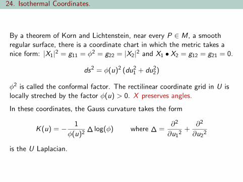
24. Isothermal Coordinates.

By a theorem of Korn and Lichtenstein, near every P ∈ M, a smoothregular surface, there is a coordinate chart in which the metric takes anice form: |X1|2 = g11 = φ2 = g22 = |X2|2 and X1 • X2 = g12 = g21 = 0.

ds2 = φ(u)2 (du21 + du2

2)

φ2 is called the conformal factor. The rectilinear coordinate grid in U islocally streched by the factor φ(u) > 0. X preserves angles.

In these coordinates, the Gauss curvature takes the form

K (u) = − 1

φ(u)2∆ log(φ) where ∆ =

∂2

∂u12

+∂2

∂u22

is the U Laplacian.

25. Stereographic Projection of the Sphere.

Figure: Stereographic Projection.P = σ(u1, u2) is the point on thesphere corresponding to(u1, u2) ∈ R2.

For the unit sphere S2 centered at theorigin, imagine a line through the southpole Q and some other point P ∈ S2.This line crosses the z = 0 plane atsome coordinate x = u1 and y = u2.Then we can express P in terms of(u1, u2). Thus σ : U = R2 → S2 − Qis a coordinate chart for the spherecalled stereographic coordinates.σ(u1, u2) =(

2u1

1+u21+u2

2, 2u2

1+u21+u2

2,

1−u21−u2

2

1+u21+u2

2

)

26. Stereographic Projection of the Sphere.-

The tangent vectors for stereographic projection are

X1 =

(2−2u2

1+2u22

(1+u21+u2

2)2 ,− 4u1u2

(1+u21+u2

2)2 ,− 4u1

(1+u21+u2

2)2

),

X2 =

(− 4u1u2

(1+u21+u2

2)2 ,

2+2u21−2u2

2

(1+u21+u2

2)2 ,− 4u2

(1+u21+u2

2)2

)so that (u1, u2) are isothermal coordinates

X1 • X2 = 0, φ(u1, u2) =√

X1 • X1 =√

X2 • X2 =2

1 + u21 + u2

2

.

Thus

K = − 1

φ2 ∆ log(φ) = 1.

27. Complex Notation for Isothermal Charts.

Figure: Transition between two isothermal coordinate charts.

Let two overlapping isothermal charts be given, σ : U → S , σ : U → Swith corresponding conformal factors

φ(z)2 |dz |2 = σ∗(ds2), φ(z)2 |dz |2 = σ∗

(ds2).

Written in complex notation, z = x + iy so |dz |2 = dx2 + dy2.

28. Intrinsic Geometry.-

The induced metrics are consistently defined. The transition functiong : U → U given by g = σ−1 σ turns out to be holomorphic (iforientation preserved) since angles are preserved. The transition identifieslocal metrics by a change of variables

φ(z)2 |dz |2 = φ(g(z))2∣∣∣∣dg

dz

∣∣∣∣2 |dz |2 = g∗(φ(z)2 |dz |2

).

Thus, oriented surfaces with a Riemannian metric have the structure of aRiemann Surface.

We don’t need to embed the surface in Euclidean Space as long as wehave a cover S by charts and define the INTRINSIC METRIC of Schartwise in a consistent way.

29. Intrinsic Metric and Distance.

The Riemannian metric gives length and angles of vectors and lengths ofcurves. If γ : [α, β] → S then γ(t) = σ(u(t)) so in the conformal metric,

L(γ) =

∫ β

αφ(u(t)

)|u(t)| dt.

The Riemannian metric induces a distance function on S . If P,Q ∈ S ,

d(P,Q) = inf

L(γ) :

γ : [α, β] → S is piecewise C 1,γ(α) = P, γ(β) = Q

Theorem

(S , d) is a metric space.

30. Hyperbolic Space invented to show independence of 5th Postulate.

Euclid’s Postulates are the following:

1 any two points may be joined by a line segment;

2 any line segment may be extended to form a line;

3 a circle may be drawn with any given center and distance;

4 any two right angles are equal;

5 (Playfair’s Version) Given any line m and a point p, there is aunique line through p and parallel to m.

31. Saccheri’s Axiom. Example of Gauss, Bolyai & Lobachevski.

Figure: m′ and m′′ are parallels tom through P. This is Poincare’smodel of the Hyperbolic Plane H2.The space is the unit disk. Lines arediameters or arcs of circles that areperpendicular to the boundarycircle.

In letters found after his death, Gausshad already realized in 1816 that thereare geometries in which the FifthPostulate fails. J. Bolyai andN. Lobachevski independently proved itin 1823 and 1826 by essentiallyconstructing Poincare’s model. Theyassumed an axiom of Saccheri, whotried to reach a contradiction from it toprove the Fifth postulate.

5 Given any line m and a point p notin m, there are at least two linesthrough p and parallel to m.

This axiom is also known as thehyperbolic axiom. In 1854, Riemannshowed a consistent geometry may alsobe constructed assuming instead thatno lines are parallel.

32. The metric of the Poincare’s Model. H2 = (D, ds2).

Let D = z ∈ C : |z | < 1 be the unit disk. The Poincare metric is

ds2 = φ(z)2 |dz |2 where φ(z) =2

1− |z |2.

Thus

K = − 1

φ2 ∆ log(φ) = −1.

Theorem (Hilbert, 1901)

There is no C 2 isometric immersion σ : H2 → E3.

The metric is invariant under rotation about the origin z 7→ e iαz (α ∈ R)and reflection z 7→ z . It is also invariant under the holomorphic self-mapsof D. Such maps f : D → D that fix the circle and map p ∈ D to 0 havethe form

w = f (z) =e iα(z − p)

1− pz

33. The metric of the Poincare’s Model.

They are isometries of the Poincare plane because the pulled-back metric

f ∗(ds2) = φ(w)2|dw |2

=4(

1− |z−p|2|1−pz|2

)2

(1− |p|2)2|dz |2

|1− pz |4

=4(1− |p|2)2|dz |2

(|1− pz |2 − |z − p|2)2

=4(1− |p|2)2|dz |2(

(1− pz)(1− pz)− (z − p)(z − p))2

=4(1− |p|2)2|dz |2(

1− pz − pz + |p|2|z |2 − |z |2 + pz + pz − |p|2)2

=4(1− |p|2)2|dz |2

(1− |p|2)2(1− |z |2)2=

4|dz |2

(1− |z |2)2= φ(z)2|dz |2.

34. Geodesics.

A geodesic is a curve that locally minimizes the length. A Calculus ofVariations argument shows geodesics satisfy a 2nd order ODE.

If ζ : [a, b] → U is minimizing in an isothermic patch, and η : [a, b] → Cis a variation such that η(a) = η(b) = 0, then the length L (σ(ζ + εη)) isleast when ε = 0 so

0 =d

dε

∣∣∣∣ε=0

L(ζ + εη) =d

dε

∣∣∣∣ε=0

∫ b

aφ(ζ + εη)

∣∣∣ζ(t) + εη(t)∣∣∣ dt

=

(∫ b

a∇φ(ζ + εη) • η|ζ + εη|+ φ(ζ + εη)

(ζ + εη) • η|ζ + εη|

dt

)∣∣∣∣∣ε=0

=

∫ b

a

(∇φ(ζ)|ζ| − d

dt

[φ(ζ)

ζ

|ζ|

])• η

35. The geodesic equation.

Since η is arbitrary, we deduce the Euler-Lagrange Equations. Thegeodesic satisfies the 2nd order ODE system

d

dt

[φ(ζ)

ζ

|ζ|

]−∇φ(ζ)|ζ| = 0. (3)

Combining ODE existence theorems with some geometry one gets

Theorem

For every P ∈ S there is a neighborhood U such that if Q1,Q2 ∈ U therethere is a unique smooth distance realizing curve ζ : [α, β] → S from Q1

to Q2 such that d(Q1,Q2) = L(ζ), ζ([α, β]) ⊂ U and ζ satisfies (3).Moreover, solutions of (3) are locally distance realizing.

36. Geodesics in H2 example.

For example, in H2, ζ(t) = (t, 0) is geodesic. |ζ| = 1,

φ(ζ(t)

)=

2

1− t2, ∇φ =

4(u, v)

(1− u2 − v2)2.

Substitutingd

dt

[2(1, 0)

1− t2

]− 4(t, 0)

(1− t2)2= 0.

37. Geodesic equation for unit speed curves.

The length is independent of parametrization. Thus we may convert toarclength

s =

∫ t

αφ(ζ(t)

)|ζ(t)| dt

so

φ|ζ| dds

=d

dt, φζ ′ =

ζ

|ζ|,

writing “ ′ ” for arclength derivatives.

d

ds

[φ(ζ)

ζ

|ζ|

]−∇ lnφ(ζ)

orζ ′′ + 2(∇ lnφ • ζ ′)ζ ′ − |ζ ′|2∇ lnφ = 0. (4)

For example, in E2, φ ≡ 1 so ζ ′′ = 0 and ζ(s) = c0 + c1s: geodesics arestraight lines. Note that any solution of (4) moves at a constant speedbecause φ(ζ)|ζ ′| remains constant.

38. Completeness.

We shall assume our surfaces are complete. The geodesic equation is

ζ ′′ + 2(∇ lnφ • ζ ′)ζ ′ − |ζ ′|2∇ lnφ = 0. (5)

S is complete if solutions of the initial value problem for (5) can beinfinitely extended.

Theorem (Hopf - Rinow)

S is complete if and only if (S , d) with the induced distance is acomplete metric space. Completeness implies that for all Q1,Q2 ∈ Sthere there is a distance realizing geodesic ζ : [α, β] → S from Q1 to Q2

such that d(Q1,Q2) = L(ζ).

39. Polar Coordinates and the Exponential Map.

Figure: Exponential Map.

The solvability, uniqueness andsmooth dependence of the initialvalue problem for (5) lets usdefine the exponential map

expP : TpM → M.

Fix P ∈ M. The map takes avector V ∈ TPM with length rand maps it to the endpoint of a

geodesic of length r which starts at Pand heads in the direction V . (So ifr = φ(p)|V |, let ζ(t) be the solution ofthe initial value problem for (5) withstarting point ζ(0) = P and directionζ ′(0) = V

r . Define expP(V ) = ζ(r).)

The exponential map gives polarcoordinates (also called normalcoordinates) near P. If M is a surfacethen a unit vector U(θ) ∈ TPM isdetermined by its angle θ. Thus anyvector V ∈ TPM can be writtenV = rU(θ) for some unit vector U(θ)and scalar r ≥ 0. The coordinate chartnear P is

σ(r , θ) = expP

(rU(θ)

).

40. The Metric in Polar Coordinates.

The metric of M in polar coordinates turns out to be

ds2 = dr2 + J(r , θ)2 dθ (6)

where J ≥ 0 in U .(The fact that circles of radius r about P cross the geodesic raysemanating from P orthogonally, hence no cross term, is a lemma ofGauss.)

In these coordinates, the Gauss Curvature is

K = −Jrr

J.

It follows that the expansion of the area growth of the r -ball near r = 0has the Euclidean value with a correction due to the Gauss curvature

A(B(0, r)

)= πr2

(1− K (P) r2

12+ · · ·

)

41. Polar Coordinates in H2 example.

For example, if P = 0 in H2 then the length of the segment from (0, 0)to (t, 0) in H2 is

ρ =

∫ t

0

2 dt

1− t2= ln

(1 + t

1− t

)⇐⇒ t = tanh

(ρ2

).

The exponential map takes (ρ, θ) in polar coordinates of E2 = TPH2 to(t, θ) ∈ H2. Pulling back the Poincare metric

dρ2+sinh2ρ dθ2 =sech4

(ρ2

)dρ2 + 4 tanh2

(ρ2

)dθ2(

1− tanh2(ρ

2

))2 = exp∗P

(4(dt2 + t2dθ2)

(1− t2)2

)

Thus

K = −Jrr

J= − 1

sinh ρ

∂2

∂ρ2sinh ρ = −1.

42. Area of a disk. Length of a circle.

In polar coordinates, H2 = (R2, dρ2 + sinh2ρ dθ2 ). Let B(0, r) be thedisk about the origin of radius r (measured in H2.). Then

L(∂B(0, r)

)=

∫ 2π

0sinh r dθ = 2π sinh r ,

A(B(0, r)

)=

∫ 2π

0

∫ r

0sinh r dr dθ = 2π(cosh r − 1).

The Taylor expansion near r = 0 gives

A(B(0, r)

)= πr2

(1 +

r2

12+ · · ·

)= πr2

(1− K (0) r2

12+ · · ·

)thus K (0) = −1.

43. Polar coordinates for general surfaces.

If S is complete, then expp : TPS → S is onto. Let e1, e2 ∈ TpS beorthonormal vectors. Let U(θ) = cos(θ)e1 + sin(θ)e2. Consider the unitspeed geodesic γ(t, θ) = expP(tU(θ)) from P in the U(θ) dierection. Foreach r > 0 let Θ(r) ∈ S1 be the set of directions θ such that γ(•, θ) isminimizing over [0, r ].

Thus if r1 < r2 we have Θ(r2) ⊂ Θ(r1). Let U = ∪r>0rU(Θ(r)). It turnsout that expP(U) covers all of S except for a set of measure zero.

44. Jacobi Equation.

The variation vector field measures the spread of geodesics as they arerotated about P ∈ S .

V =d

dθγ(t, θ) (7)

is perpendicular to γ(t, θ) and has length J(t, θ) as in the metric in polarcoordinates (6). By differentiating the geodesic equation (5) with respectto θ one finds the Jacobi Equation

Jss(s, θ) + K(γ(s, θ)

)J(s, θ) = 0 (8)

with initial conditions, J(0, θ) = 0 and Js(0, θ) = 1.

For example, in H2, J(s, θ) = sinh s and K ≡ −1.For E2, J(s, θ) = s and K ≡ 0.

45. Harmonic functions.

Let ds2 = φ(z)2 |dz |2 be the metric in an isothermal coordinate patch.The intrinsic area form, gradient and Laplacian are given by the formulas

dA = φ2 dx dy ; |∇u|2 =u2x + u2

y

φ2; ∆u =

uxx + uyy

φ2=

4uzz

φ2.

Let u ∈ C 1(Ω) be a function on a domain Ω ⊂ S . Then the energy orDirichlet integral is invariant under conformal change of metric∫

Ω|∇u|2 dA =

∫Ω

u2x + u2

y dx dy .

A function is harmonic if ∆u = 0 and subharmonic if ∆u ≥ 0 (at leastweakly.) These notions agree regardless of conformal metric φ2 |dz |2.

46. Parabolicity.

We seek generalizations of the Riemann mapping theorem to surfaces.

Theorem (Riemann Mapping Theorem)

Let Ω ⊂ R2 be a simply connected open set that is not the whole plane.Then there is an analytic, one-to-one mapping onto the disk f : Ω → D.

A noncompact, simply connected surface S is said to be parabolic if it isconformally equivalent to the plane. That is, there is a global isothermalcoordinate chart σ : C → S . Otherwise the surface is called hyperbolic.The sphere S2 is compact, so it is neither parabolic nor hyperbolic.

Theorem (Koebe’s Uniformization Theorem)

Let S be a simply connected Riemann Surface. Then S is conformallyequivalent to the disk, the plane or to the sphere.

Conceivably, the topological disk could have many conformal structures,but the uniformization theorem tells us there are only two. Thetopological sphere has only one conformal structure.

47. Characterizing hyperbolic manifolds.

For each p ∈ S , the positive Green’s function z 7→ g(z , p) is harmonic forz ∈ S − p, g(z , p) > 0, infz g(z , p) = 0 and in a isothermal patcharound p, g(z , p) + ln |z − p| has a harmonic extension to aneighborhood of p (so g(z , p) →∞ as z → p.)

Theorem

Let S be a simply connected noncompact Riemann surface. Then thefollowing are equivalent.

S is hyperbolic.

S has a positive Green’s function.

S has a negative nonconstant subharmonic function.

S has a bounded nonconstant harmonic function.

e. g., u = ax + by is a bounded harmonic function on D hence on H2,but there are no bounded harmonic functions on E2 by Liouville’sTheorem.

48. A theorem relating curvature and function theory.

A surface S is said to have finite total curvature if∫S|K | dA <∞.

Theorem (Blanc & Fiala, Huber)

Let S be a noncompact, complete surface with finite total curvature.Then S is conformally equivalent to a closed Riemann surface of genus gwith finitely many punctures Σg − p1, . . . , pk.

For example, E2 has zero total curvature and is conformal to S2 − Qvia stereographic projection.

To illustrate something of the ways of geometric analysis, we sketch theproof for the simply connected case.

49. Growth of a geodesic circle.

Lemma

Assume that S is a complete, noncompact, simply connected surfacewith finite total curvature ∫

S|K | dA = C <∞.

ThenL(∂B(p, r)

)≤ (2π + C )r .

Proof Idea. By the Jacobi equation (7),

Jr (r , θ)− 1 = Jr (r , θ)− Jr (0, θ)

=

∫ r

0Jrr (r , θ) dr

= −∫ r

0K(γ(r , θ)

)J(r , θ) dr .

50. Growth of a geodesic circle proof.

The length L(r) = L(∂B(p, r)

)grows at a rate

dL

dr= lim

h→0+

L(r + h)− L(r)

h

= limh→0+

1

h

(∫Θ(r+h)

J(r + h, θ) dθ −∫

Θ(r)J(r , θ) dθ

)

= limh→0+

(∫Θ(r+h)

J(r + h, θ)− J(r , θ)

hdθ − 1

h

∫Θ(r)−Θ(r+h)

J(r , θ) dθ

)

≤∫

Θ(r)Jr (r , θ) dθ

=

∫Θ(r)

(1−

∫ r

0K(γ(r , θ)

)J(r , θ) dr

)dθ

≤ 2π +

∫ r

0

∫Θ(r)

∣∣K(γ(r , θ))∣∣ J(r , θ) dθ dr

= 2π +

∫B(P,r)

|K | dA ≤ 2π + C .

51. Blanc & Fiala’s theorem.

Theorem (Blanc & Fiala)

Let S be a complete, noncompact, simply connected Riemann surface offinite total curvature. Then S is parabolic.

Proof idea. Suppose not. Then S has a global isothermal chartσ : D → S . Then u = − ln |z | is a positive Green’s function on S . Letε > 0 and K ⊂ D− B(0, ε) be any compact domain. On the one hand,the energy is uniformly bounded

E(K ) =

∫K

u2x + u2

y dx dy ≤ −2π ln ε.

This estimate is done in the background D metric. But energy isconformally invariant, so it will hold in the surface metric also.

52. Blanc & Fiala’s theorem. -

Indeed, let R = sup|z | : z ∈ K < 1 and A = z ∈ D : ε ≤ |z | ≤ R bean annulus containing K . Using the fact that u > 0 and ur < 0 on K , byintegrating by parts,

E(K ) ≤ E(A) = −∫A

u∆0u dx dy +

∮|z|=ε

u∂u

∂n+

∮|z|=R

u∂u

∂n

≤ 0−∮|z|=ε

ln ε

ε+ 0

≤ −2π ln ε

since on |z | = ε, u = − ln ε and ur = −1ε and L(z : |z | = ε) = 2πε.

53. Blanc & Fiala’s theorem. - -

On the other hand, bounded total curvature will imply that the energywill grow to infinity. For the remainder of the argument, work in intrinsicpolar coordinates. Let B(0, r) denote the intrinsic ball for r ≥ 1 and

E(r) =

∫B(0,r)−B(0,1)

|Du|2 dA =

∫ r

1

∫∂B(0,r)

|Du|2 ds dr

where s is length along ∂B(0, r). By the Schwartz inequality,

L(r)dEdr

=

∫∂B(0,r)

ds

∫∂B(0,r)

|Du|2 ds ≥

(∫∂B(0,r)

|Du| ds

)2

≥

(∮∂B(0,r)

∂u

∂n

)2

=

(∫B(0,r)−B(0,δ)

∆u dA−∮

∂B(0,δ)

∂u

∂n

)2

= c0

for any fixed δ ∈ (0, 1] where c0 > 0 is independent of r .In fact, c0 → 4π2 as δ → 0.

54. Blanc & Fiala’s theorem. - - -

Now, using the length lemma,

dEdr

≥ c0

(2π + C )r.

Integrating, this says

E(r) ≥ c0 ln r

(2π + C )→∞ as r →∞.

This is a contradiction because the energy is invariant under conformalchange and is uniformly bounded.

To understand the argument, try using it to prove E2 is parabolic!

55. Application to harmonic maps.

A harmonic map locally minimizes energy of a map between surfaces,generalizing harmonic functions and geodesics.If h : (S1, φ(z)2 |dz |2) → (S2, ψ(w)2 |dw |2) is harmonic, then it satisfiesthe PDE system

hzz + 2ψw (h)

ψ(h)hz hz = 0.

Theorem

If f : S → S1 is a conformal diffeomorphism and h : S1 → S2 is harmonic,then h f : S → S2 is harmonic.

56. Existence of harmonic diffeomorphisms.

Theorem (Treibergs 1986)

Let I ⊂ ∂D be any closed set with at least three distinct points andConv(I) its convex hull in H2, then there is a complete, spacelike entireconstant mean curvature surface S in Minkowski Space such that theGauss map G : S → Conv(I) is a harmonic diffeomorphism.

Minkowski Space is E2,1 = (R3, dx2 + dy2 − dz2).An entire, spacelike surface S ⊂ E2,1 is the graph of a functionS =

(x , y , u(x , y)

): (x , y) ∈ R2

such that u2

x + u2y < 1.

The Gauss map is the map given by the future-pointing unit normal

G =(ux , uy , 1)√1− u2

x − u2y

: S → H.

The hyperboloid H = (x , y , x) : x2 + y2 − z2 = −1, z > 0 consists ofall future-pointing vectors of length −1.The hyperboloid model (H, dx2 + dy2 − dz2) is isometric to H2.

57. Harmonic diffeomorphisms Conv(I).

Figure: Harmonic diffeomorphisms

58. Harmonic diffeomorphisms to ideal polygons.

Corollary

Let I ⊂ ∂B be a closed set with at least three points.

If I is finite, there is a harmonic diffeomorphism

h : C → Conv(I).

If I has nonempty interior, then there is a harmonic diffeomorphism

h : B → Conv(I).

Since S is convex, its total curvature is −A(G(S)

)= π(2− ]I) by the

Gauss-Bonnet Theorem in H2. By Blanc-Fiala’s Theorem, S is conformalto the plane if I is finite.

If I has nonempty interior then one can construct a nonconstantbounded harmonic function on S so it is conformal to the disk.

Thanks!