geometry of algebraic curves - university of …math.uchicago.edu/~amathew/287y.pdfgeometry of...
TRANSCRIPT

Geometry of Algebraic Curves
Lectures delivered by Joe HarrisNotes by Akhil Mathew
Fall 2011, Harvard
Contents
Lecture 1 9/2§1 Introduction 5 §2 Topics 5 §3 Basics 6 §4 Homework 11
Lecture 2 9/7§1 Riemann surfaces associated to a polynomial 11 §2 IOUs from last time: the
degree of KX , the Riemann-Hurwitz relation 13 §3 Maps to projective space 15 §4Trefoils 16
Lecture 3 9/9§1 The criterion for very ampleness 17 §2 Hyperelliptic curves 18 §3 Properties
of projective varieties 19 §4 The adjunction formula 20 §5 Starting the courseproper 21
Lecture 4 9/12§1 Motivation 23 §2 A really horrible answer 24 §3 Plane curves birational to
a given curve 25 §4 Statement of the result 26
Lecture 5 9/16§1 Homework 27 §2 Abel’s theorem 27 §3 Consequences of Abel’s theorem 29§4 Curves of genus one 31 §5 Genus two, beginnings 32
Lecture 6 9/21§1 Differentials on smooth plane curves 34 §2 The more general problem 36 §3
Differentials on general curves 37 §4 Finding L(D) on a general curve 39
Lecture 7 9/23§1 More on L(D) 40 §2 Riemann-Roch 41 §3 Sheaf cohomology 43
Lecture 8 9/28§1 Divisors for g = 3; hyperelliptic curves 46 §2 g = 4 48 §3 g = 5 50
1

Lecture 9 9/30§1 Low genus examples 51 §2 The Hurwitz bound 52
2.1 Step 1 . . . . . . . . . . . . . . . . . . . . . . . . . . . . . . . . . 532.2 Step 1′ . . . . . . . . . . . . . . . . . . . . . . . . . . . . . . . . . 542.3 Step 1′′ . . . . . . . . . . . . . . . . . . . . . . . . . . . . . . . . 542.4 Step 2 . . . . . . . . . . . . . . . . . . . . . . . . . . . . . . . . . 54
Lecture 10 10/7§1 Preliminary remarks 57 §2 The next theorem 57 §3 Remarks 58 §4 The
main result 59
Lecture 11 10/12§1 Recap 62 §2 The bound, again 64 §3 The general position lemma 64 §4
Monodromy 65 §5 Proof of the general position lemma 66
Lecture 12 10/14§1 General position lemma 68 §2 Projective normality 69 §3 Sharpness of the
Castelnuovo bound 70 §4 Scrolls 71
Lecture 13 10/17§1 Motivation 74 §2 Scrolls again 75 §3 Intersection numbers 75
Lecture 14 10/19§1 A basic lemma 79 §2 Castelnuovo’s lemma 81 §3 Equality in the Castelnuovo
bound 82
Lecture 15 10/21§1 Introduction 84 §2 Castelnuovo’s argument in the second case 85 §3
Converses 87
Lecture 16 10/26§1 Goals 89 §2 Inflection points 90 §3 A modern reformulation 91
Lecture 17 11/2§1 Review 95 §2 The Gauss map 96 §3 Plane curves 97
Lecture 18 11/4§1 Inflectionary points; one last remark 101 §2 Weierstrass points 102 §3 Examples 105
Lecture 19 11/9§1 Real algebraic curves 106 §2 Singularities 108 §3 Harnack’s theorem 108 §4
Nesting 109 §5 Proof of Harnack’s theorem 110
Lecture 20 11/16§1 Basic notions 111 §2 The differential of u 112 §3 Marten’s theorem 115

Lecture 21 11/18§1 Setting things up again 116 §2 Theorems 118
Lecture 22 11/30§1 Recap 121 §2 Families 122 §3 The basic construction 123 §4 Constructing
such families 124 §5 Specializing linear series 125
Lecture 23 12/2§1 Two special cases 127 §2 The inductive step 128 §3 The basic construction 128§4 A relation between the ramifications of U,W 130 §5 Finishing 131

Introduction
Joe Harris taught a course (Math 287y) on the geometry of algebraic curves at Harvardin Fall 2011. These are my “live-TEXed” notes from the course.
Conventions are as follows: Each lecture gets its own “chapter,” and appears in thetable of contents with the date. Some lectures are marked “section,” which means thatthey were taken at a recitation session. The recitation sessions were taught by AnandDeopurkar.
Of course, these notes are not a faithful representation of the course, either in themathematics itself or in the quotes, jokes, and philosophical musings; in particular, theerrors are my fault. By the same token, any virtues in the notes are to be credited tothe lecturer and not the scribe.
Please email corrections to [email protected].
Lecture 1 Geometry of Algebraic Curves notes
Lecture 19/2
§1 Introduction
The text for this course is volume 1 of Arborello-Cornalba-Griffiths-Harris, which iseven more expensive nowadays.
We will be covering a subset of the book, and probably adding some additionaltopics, but this will be the basic source for most of the stuff we do. There will beweekly homeworks, and that will determine the grade for those of you taking thecourse for a grade. There will be no final.
There will be a weekly section with Anand Deopurkar.The course doesn’t meet on Mondays because of the “Basic Notions” seminar. On
those weeks that there won’t be seminars, we might meet then. Every third or fourthweek, the lecture will be cut short on Wednesdays. However, the course will basicallymeet on a three-hour-per-week basis.
§2 Topics
Here is what we are going to talk about. We are going to talk about compact Riemannsurfaces, and a compact Riemann surface is the same thing as a smooth projectivealgebraic curve (over C). That in turn is really the same thing as a smooth projectivecurve over any algebraically closed field of characteristic zero. By abuse of notation,we will use C to denote any such field as well.
The fact that these are the same thing—that is, that a compact Riemann surfaceis an algebraic curve—is nontrivial. It requires work to show that such an object evenadmits a nontrivial meromorphic function. Note:
1.1 Proposition. There are compact complex manifolds of dim ≥ 2 that do not admitnonconstant meromorphic functions.
The miracle in dimension one is that there are nonconstant meromorphic functions,and enough to embed the manifold in projective space.
There are a number of beautiful topics that we are not going to cover. We will nottalk about singular algebraic curves, in general. We will encounter them (e.g. whenwe consider maps of curves to projective space, the image might be singular), but theywill not be the focus of study. When we have a singular curve C in projective space,we will treat C its normalization, i.e. as an image of a smooth projective curves. Wealso will not talk about open (i.e. noncompact) Riemann surfaces. Another even-more large-scale and interesting topic is the theory of families of curves, and how theisomorphism class of a curve changes as we vary the coefficients of the defining equations(e.g. moduli of curves). Finally, we are not going to talk about curves over fields thatare not algebraically closed. There has been a huge amount of work on algebraic curvesover R, but we won’t discuss them.
5

Lecture 1 Geometry of Algebraic Curves notes
§3 Basics
Today, we shall set the notation and conventions. Algebraic curves is one of the oldestsubjects in modern mathematics, as it was one of the first things people did once theylearned about polynomials. It has developed over time a multiplicity of language andsymbols, and we will run through it.
Let X be a smooth projective algebraic curve over C. There are many ways ofdefining the genus of X, e.g. via the Hilbert polynomial, the Euler characteristic (viacoherent cohomology), and so on. We are just going to take the naive point of view.
1.2 Definition. The genus of X is the topological genus (as a surface).
We can also use:
1. g(X) = 1− χ(OX).
2. 1− 12χtop(X).
3. 12 degKX + 1 (for KX the canonical divisor, see below).
Given a geometric object, one wishes to define the functions on it. On a compactRiemann surface, there are no nonconstant regular functions, by the maximal principle:every holomorphic function on X is constant. We need to allow poles, and to keep trackof them we will need to introduce the language of divisors.
1.3 Definition. A divisor D on X is a formal finite linear combination of points∑nipi, pi ∈ X on the curve. We say that D is effective if all ni ≥ 0 (in which case
we write D ≥ 0), and we say that degD =∑ni is the degree of D.
As a reality check, one should see that the family of effective divisors of a givendegree d should be the dth symmetric power of the curve with itself, Cd; this is C ×· · · × C (d times) modulo the symmetric group Sd.
The point of this is, if we have a meromorphic function f : X → P1, we can associateto it a divisor measuring its zeros and poles.
1.4 Definition. Given f : X → P1, we say that the divisor of X is the sum∑p∈X ordp(f)p. The positive terms come from the zeros, while the negative terms
come from the poles.
The problem is to deal with interesting classes of functions. Holomorphic functionsdo it, while there are too many meromorphic functions to work with them all at once.Instead, we do the following:
1.5 Definition. Given a divisor D =∑npp, we can look at functions which may have
poles at each p, but with orders bounded by np. Namely, we look at the space L(D)of rational functions f : X → P1 such that ordp(f) ≥ −np for all p ∈ X. This isequivalently the space of f such that div(f) +D ≥ 0.
We note (without proof) that L(D) is finite-dimensional. We write:
1.6 Definition. 1. `(D) = dimL(D).
6

Lecture 1 Geometry of Algebraic Curves notes
2. r(D) = `(D)− 1.
In the literature, both notations `, r are used.The basic problem is this: given D, find explicitly these vector spaces L(D), and
in particular the dimension `(D) and the number r(D). This is a completely solvedproblem, and not just by general theorems like Riemann-Roch. If one is given analgebraic curves as a smooth projective curve (given by explicit equations), and anexplicit divisor, there is an algorithm to determine the space L(D). We’ll do that in aweek or two.
The one thing to observe is that there’s a certain redundancy here, in this problem.This is for the following reason: if L(D) is known, and E is another divisor that differsfrom D by div(f) for some global meromorphic f : X → P1 (nonconstant), then wecan determine L(E). Namely, there is an elementary isomorphism
L(D) ' L(E),
given by multiplying by the rational function f . So, in some sense, asking to describeL(D) is the same as asking to describe L(E). To solve this problem, we need onlystudy divisors modulo this equivalence relation.
1.7 Definition. We say that D,E are linearly equivalent when there is a globalmeromorphic function f such that D − E = div(f). We write D ∼ E.
In some sense, the fundamental object is the space of divisors modulo linear equiva-lence. Note that the degree of a global rational function is zero, so the degree is definedmodulo linear equivalence. (This states that the number of poles is the same as thenumber of zeros, for a global meromorphic functions.)
We are going to realize the space of divisors modulo linear equivalence as a space.For now:
1.8 Definition. We call Picd(X) the space of divisors on X modulo linear equivalence.
So far, we’re just talking about divisors in general on X. There is a particular onewe should keep in mind, the canonical divisor.
1.9 Definition. If ω is a meromorphic 1-form (i.e., something that locally looks likef(z)dz for a meromorphic function f), we can define the order at a point p ∈ X (viathe order of the coefficient function). In particular, we can define the divisor div(ω)of a meromorphic 1-form ω.
Note that the ratio of two meromorphic 1-forms ω1, ω2 is a global meromorphic (orrational) function ω2/ω1. In particular, div(ω1) = div(ω2).
The canonical class KX of X is the class of the divisor of ω for any meromorphic1-form ω.
We’re now going to turn around and say everything again, in a more modern lan-guage.
There are a lot of circumstances in which we want to forget about the divisor D, andthink only of linear equivalence. We would like a terminology that would let us onlyspecify the divisor mod linear equivalence. This will be the language of line bundles.
7
Lecture 1 Geometry of Algebraic Curves notes
1.10 Definition. Suppose D =∑npp is a divisor on X. Let OX be the sheaf of
regular functions on X; similarly, we define OX(D) to be the sheaf of functions withzeros and poles prescribed by this divisor D. In other words, the sections of OX(D) overan open subset U are the meromorphic functions f : U → P1 such that ordp(f) ≥ npfor p ∈ U .
This is a local version of the space L(D) (i.e. L(D) = Γ(X,OX(D)), and is muchlarger.
The point is that this sheaf OX(D) is locally free of rank one. In other words, itis a holomorphic line bundle. We will basically identify holomorphic line bundles withlocally free sheaves of OX -modules of rank one; this is standard in algebraic geometry.
Remark. If D ∼ E, then OX(D) ' OX(E) as line bundles. So, in some sense, we canrealize the space of divisors modulo linear equivalence as the space of line bundles onX. That’s how Picd(X) is typically defined.
There’s one more thing we should define. There is a canonical divisor class, andthe associated line bundle can be easily defined. Namely, we just have to take theholomorphic cotangent bundle T ∗X ; this corresponds to the divisor associated to anyglobal meromorphic 1-form.
We said at the outset that compact Riemann surfaces correspond to smooth pro-jective curves. How do we go from one to another? How do we describe maps from Xto projective space Pn? This is where the notion of divisors and line bundles plays anessential role. We could write all this in the classical language of divisors, but we’ll usethe modern language of line bundles; you can think in the former way if you wish.
Let L be a line bundle on X. Suppose σ0, . . . , σr are global sections of L, saylinearly independent. (So if L = OX(D), then each σi corresponds to an element ofL(D), i.e. a meromorphic function on X with appropriate zeros and poles.) Supposethat they have no common zeros. In that case, there is induced a map
X → Pr, x 7→ [σ0(x), . . . , σr(x)].
Here the σi(x) sure aren’t numbers, but we can still make sense of this. Namely, the σiare not numbers, but they are elements of the fiber of L over p. Given an r+1-tuple ofelements of a one-dimensional C-vector space, we get a uniquely determined element ofPr. Another way to see it is that a line bundle is locally trivial, and we can use a localtrivialization to think of the σi(x) as functions so that the σi(x) are actual numbers. Ifyou chose a different trivialization, you would get a different vector [σ0(x), . . . , σr(x)],but it would be the same up to scalars. In fact, if we changed the σi around, then wewould just change the embedding by some automorphism group of Pn.
So,
Up to automorphisms of Pn, the map X → Pr is uniquely determined bythe subspace of H0(L) spanned by the {σi}.
We thus get:
1.11 Proposition. There is a correspondence between pairs (L, V ) where L is a linebundle on X of degree d and V ⊂ H0(L) is an r+ 1-dimensional space of sections with
8

Lecture 1 Geometry of Algebraic Curves notes
no common zeros, and the space of nondegenerate maps of degree d, X → Pr (up toautomorphisms of Pr).
So if we’re looking for maps to projective space, it’s the same as looking for linebundles and sections. Here the word “nondegenerate” means that the image is notcontained in a hyperplane. If the image is contained in a hyperplane, then the sectionsσ1, . . . , σr used to define the map would satisfy a nontrivial linear relation.
1.12 Definition. A linear series of degree d and dimension r on X is a pair (L, V ):
1. L is a holomorphic line bundle on X, of degree d (i.e. the associated divisor hasdegree d).
2. V is an r + 1-dimensional space of sections, contained in H0(L).
We are no longer requiring that there be no common zeros. This is to make the spacecompact.
This will be denoted grd: here, again, the d refers to the degree, r the dimension.Here “g” comes from the old word for a divisor, a “group.”
A grd can be thought of as a family of effective divisors. For each σ ∈ V ⊂ H0(L),we can associate the divisor of zeros div(σ). This means that P(V ) corresponds to afamily of effective divisors on X, parametrized by the projective space P(V ). To recap,each nonzero section has a divisor (or divisor of zeros), and the section is defined upto rescaling by its divisor (because there are no nonconstant holomorphic functions onX). When you think of a linear series in this form, it is often denoted D .
We can give a more intrinsic description of the map associated to a linear system.Given a linear system (L, V ) on X without common zeros, we can describe the associ-ated map X → Pr as the map specifically sending X to the projectivization P(V ∗), sothat a point p ∈ X is sent to the hyperplane of sections in V vanishing on p (and thishyperplane belongs to P(V ∗)).
Lastly (and this is really crucial), when the genus of X is ≥ 1, we have enoughholomorphic differentials on X to get a map to projective space.
1.13 Proposition. The dimension of the space L(K) of holomorphic 1-forms is exactlythe genus g. Moreover, there are no common zeros of the canonical line bundle L(K),so there is a canonical map X → Pg−1 associated to the linear series of all 1-forms.
We’ve left out a lot of details (and even a lot of definitions), but now we want todo something. Let’s give a false proof of Riemann-Roch in the next five minutes.
Given a divisor D, we’re (as before) interested in the space L(D) of rational func-tions with the desired poles. Suppose for simplicity D is a sum of distinct points,D = p1 + p2 + · · ·+ pd. The vector space L(D) consists of meromorphic functions thathave at most a simple pole at the points pi but are otherwise regular. How might youdefine such a function?
Choose a local coordinate zi around pi; given a function f ∈ L(D), we can write itnear pi as ai
zi+ f0 for some holomorphic f0 (defined in a neighborhood of pi), because
f is only allowed to have simple poles. This polar part aizi
says a lot about f . In fact,f is determined up to addition of scalars by specifying these polar parts {ai}, again
9
Lecture 1 Geometry of Algebraic Curves notes
because there are no nonconstant holomorphic functions on X. In other words, thereis a natural map
L(D)→ Cd,
whose kernel consists of the constant functions. We get in particular,
`(D) ≤ 1 + d.
If you want to describe L(D) (and in particular its dimension), you want to know theimage. This raises the question:
Given a1, . . . , ad, when is there a global meromorphic f : X → P1 withpolar part ai
ziat pi, and holomorphic elsewhere?
In other words, we need to find constraints on the {ai} for them to form a family ofpolar parts of a function in L(D). Here’s the point: if f ∈ L(D), and ω is a holomorphic1-form, we can consider the meromorphic differential fω. This has potentially simplepoles at the {pi}, but is holomorphic elsewhere. In particular, the sum of the residuesis zero.
(Recall that the sum of the residues of a meromorphic differential on a compactRiemann surface is zero.)
So, if ω = gi(zi)dzi locally, near pi (using the local coordinate zi around pi), then theresidue of fω at pi is aigi(pi). It follows that if the {ai} arise as a system of polar parts,then we want
∑aigi(pi) = 0. Thus the image of the map L(D) → Cd is contained
in the orthogonal complement of the space of holomorphic differentials (where each ωmaps to (gi(pi)) ∈ Cd as before). We get a total of g linear conditions on the {ai}, overa family of holomorphic differentials, suggesting that
`(D) ≤ 1 + d− g
But this is false. It’s possible that a differential might not give a serious relation onthe {ai}. For instance, a differential at the points {ai}. The correct statement is
`(D) ≤ 1 + d− (g − `(K −D)), (1)
because the dimension of the image of L(D) → Cd is contained in the orthogonalcomplement of the image of the 1-forms in Cd.
However, a 1-form is the dual of a vector field. So the degree of a 1-form is justminus the degree of the corresponding vector field, and that is the topological Eulercharacteristic. In particular, the degree of a 1-form is the opposite of the topologicalEuler characteristic, i.e. 2g − 2.
Now we want to apply (1) to K −D, and we get
`(K −D) ≤ 1 + (2g − 2− d)− g + `(D),
where we have used the degree of K to get the degree of K −D as 2g− 2− d. Now weadd this to (1). We get `(D) + `(K −D) ≤ `(K −D) + `(D), and as a result we musthave equalities in both inequalities. We “get”:
10

Lecture 2 Geometry of Algebraic Curves notes
1.14 Theorem (Riemann-Roch). For any divisor D of degree d, we have
`(D) = d− g + 1 + `(K −D).
But, we’ve been cheating. The restriction in the argument to divisors of the formp1 + · · ·+ pd was ok, but there is a serious gap in this argument.
The point, however, is that everything derives from the condition that the sum ofthe residues of a meromorphic differential be zero.
§4 Homework
Here is the homework assignment: ACGH, chapter 1, “batch A,” problems 1-5. Thiswill be due next Friday. When we talk about a “curve,” we mean the normalization ofthe compactification.
Lecture 29/7
We start with some material intended to help out with the problem set.
§1 Riemann surfaces associated to a polynomial
Consider a polynomial f(x, y) ∈ C[x, y]. We want to think of this in the form ad(x)yd+ad−1(x)yd−1 + · · · + a1(x)y + a0(x). Consider the equation that this should be set tozero. As we vary x, we want to think of there being d solutions of y. So y is a functionimplicitly defined by x, with d possible values; it varies holomorphically. A large partof the impetus for Riemann surfaces was to provide a proper foundation for such multi-valued functions. (They did not develop abstractly as compact complex manifolds ofdegree one. They came up as branched covers of P1, that occurred via multi-valuedfunctions in this way.)
We’re going to discuss this complex-analytically, to start with. Consider X ={(x, y) : f(x, y) = 0} ⊂ C2, the “complex plane” (this is very ambiguous terminology).Let X0 be the smooth locus, so X0 is a smooth submanifold of C2. We want to thinkof this as a branched cover of P1.
We have a projection map π : X → C that sends a point to its x-coordinate. Forp ∈ X, there are three possibilities:
1. π is smooth at p. That is, ∂∂yf(p) 6= 0, so X is smooth at p and π is a local
isomorphism (in the complex analytic or etale topologies).
2. ∂∂yf(p) = 0, but ∂
∂xf(p) = 0. Here X is smooth at p, but the projection mapfrom X is not locally one-to-one. So π is locally m-to-one, and in terms of localcoordinates, it looks like z 7→ zm. This is a branched cover of the disk.
In this case, we say that p is a branch point of the map, and m the ramification.
3. Both derivatives vanish, in which case we have a singular point of the curve (inX −X0). There is an algebraic answer, but here is the complex analytic answer.
11

Lecture 2 Geometry of Algebraic Curves notes
However, it doesn’t matter. No matter how bad the singularity is, we can stillfind a suitable neighborhood of the image point, such that over the punctureddisk, the associated map is a covering space. That is, if q = π(p), then there is asmall disk ∆ containing q such that π−1(∆∗)→ ∆∗ (for ∆∗ the punctured disk)is a covering. This is because singular locus is a finite set.
So, any covering of a punctured disk ∆∗, say the unit disk in the complex plane,
is given in the form ∆∗z 7→zm→ ∆∗. No matter how bad the singularity may look at
first, be assured that if one eliminates the singular point and its pre-image, thenyou just get a disjoint union of punctured disks. In this case, one fills in eachconnected component (which is a punctured disk) by adding a point (to makethese punctured disks disks). That’s it. This is a procedure that gives a newcomplex manifold that projects onto the x-line.
So, after we make the transformation in the last item, then we get a Riemannsurface projecting to the x-line. We have resolved the singularities.
2.1 Example. Consider the equation y2 − x2, projecting to the line. There is asingularity at the origin. If we take the pre-image over a punctured disk in the x-line,we get a union of two punctured disks. So the associated Riemann surface has twopoints above the origin, one for each punctured disk.
2.2 Example. Consider the curve defined by y2 − x3. We take the pre-image overthe x-punctured-disc {x : 0 < |x| < ε}. The curve looks analytically locally like onepunctured disk, so there is one point over the origin in the associated Riemann surface.
2.3 Example. Consider y3 − x2; here the x-projection is locally three-to-one. Thepre-image over a small punctured disk in the x-plane is connected, so one point liesover the origin in the Riemann surface.
So, right now we have associated a branched cover of C by a Riemann surface X toany polynomial equation P (x, y), even if this is singular (by possibly adding points).We want, however, a compact Riemann surface in the end. We take the complexnumbers C and complete it to P1. We want to extend the branched cover X → C toa branched cover X → P1 such that X is a compact Riemann surface. To do this,take the complement of a large disk, so something of the form UR = {x : |x| > R}. Letπ : X → C be the projection. Then π−1(UR) → UR is a covering space for R � 0.So we get a covering space of the punctured disk UR. Again, we can complete this toa compact Riemann surface X by adding one point in each connected component ofπ−1(UR).
In this way, we complete X to a compact Riemann surface.
2.4 Theorem. To each equation P (x, y) = 0, we can associate a branched cover X →P1 where X is a compact Riemann surface, by the above procedure.
The above construction gives a means of computing the number of points in thefiber above ∞, for instance: one has to consider the number of connected componentsin the pre-image of a large disk.
12

Lecture 2 Geometry of Algebraic Curves notes
2.5 Example. Consider y2 = x3−1. Consider this as a two-sheeted cover of the x-line.The branch points occur at the cube roots of unity. Over the complement of a largedisk in the x-line, the projection is a covering space. We only need to know whetherthe pre-image of said complement is connected.
It is. To see this, let’s wander around a bit. As x wanders around a large circleand gets back to the same point, the argument increases by 2π, so the argument ofx3 − 1 increases by 6π if we are wandering around a large circle. Thus the argumentof y increase by 3π, so y flips. It follows that the cover is connected, and one adds onepoint. (The idea is that analytically continuing a germ of a solution of y in terms of xaround a circle gives the opposite solution.)
This is a recipe. Starting with a polynomial in two variables, you arrive at a compactRiemann surface. You can do the same thing, purely algebraically. For one thing, youneed to make a complete variety (this is the algebraic way of saying “compact”), andwe also want to make it smooth. Typically, what you would do algebraically is to startwith the polynomial P (x, y), and take the associated curve in A2. We can take theclosure of this in P2, which is the hypersurface in P2 cut out by the homogeneizationby P (x, y). Then, one has to normalize the projective curve by blowing up to resolvesingularities. If you want to carry this out algebraically, here is an alternative.
Warning: Don’t do this. If you can take the analytic route, use that instead. Youmight have to blow up a curve multiple times to resolve a singularity (e.g. for a curvelike ya − xb), while the analytic approach is very simple. Moreover, the operation oftaking projective closure is not well-behaved. There is nothing to suggest that thecurve necessarily wants to live in P2: taking the projective closure even of a smoothaffine curve may give a non-smooth curve. Eye-balling polynomials and thinking aboutRiemann surfaces is easier.
§2 IOUs from last time: the degree of KX, the Riemann-Hurwitzrelation
There are several things owed from last lecture. If X is a compact Riemann surface ofgenus g, we want to claim:
2.6 Proposition. deg(KX) = 2g − 2 for KX the canonical divisor.
This is going to come out of the Riemann-Hurwitz relation. Namely, let X,Y becompact Riemann surfaces. Let g(X) = g, g(Y ) = h. Let f : X → Y be a nonconstantholomorphic map. By standard complex analysis, this means that the map f has finitedegree d. So, over all but finitely many points of Y , the pre-image has cardinality d.There will be a finite number of ramification points in X, where f will fail to be a localisomorphism. (The images of the ramification points, which lie in Y , are called thebranch points.)
2.7 Definition. Given p ∈ X mapping to q ∈ Y , we can choose local coordinates nearp, q such that f looks like f : z 7→ zm; that is, it looks like a standard m-fold cover ofa disk by a disk. In this case, we say that the ramification index is m − 1. Whenm ≥ 2, then there is ramification at p. We denote m− 1 by νp(f).
13
Lecture 2 Geometry of Algebraic Curves notes
2.8 Definition. Let R be the ramification divisor on X. This is∑
p∈X νp(f)p. Thebranch divisor B is the image of R under f . This “image” is taken in the naive sense.
So B =∑
q∈Y
(∑p∈f−1(q) νp(f)
)q.
In particular, if we write B =∑nqq, then the cardinality of f−1(q) is d−nq. When
you have ramification, you lose points in the fiber (so there will be less than d).Now we derive Riemann-Hurwitz. Consider X with all the points in the branch
divisor removed. Take q1, . . . , qδ be the points appearing in the branch locus. Weconsider X ′ = X − f−1({q1, . . . , qδ}), which maps by a covering space map to Y ′ =Y −{q1, . . . , qδ}. So X ′ → Y ′ is a d-sheeted covering space map. In particular, χ(X ′) =dχ(Y ′). We know these Euler characteristics. So χ(Y ′) = χ(Y ) − δ = 2 − 2h − δ.Similarly, χ(X ′) = χ(X)−
∑i(d− nq) for nq = |f−1(q)|, and χ(X) = 2− 2g. We have
just used the fact that removing points decreases the Euler characteristic accordingly.We are left with:
2.9 Theorem (Riemann-Hurwitz). Notation as above,
2− 2g = d(2− 2h)− deg(B).
This is often written as
g − 1 = d(h− 1)− b
2.
One way to remember this, which generalizes to higher dimensions, is that the Eulercharacteristic χ(X) upstairs is exactly what it would be if X → Y were a coveringspace—that is, dχ(Y )—with correction terms for the ramification. This in fact gener-alizes to higher dimensions, but that’s for another course.
Here’s another thing. Suppose f : X → Y is a map. Let ω be any meromorphicdifferential on Y . For simplicity, let’s assume that div(ω) is supported away from thebranch points. So there are no zeros or poles of ω on these branch points. What’s thedivisor of f∗ω? But if ω has a pole or a zero or downstairs, then pulling back gives ita pole or zero of the same degree upstairs except at the branch points. At the branchpoints, if f looks locally like z 7→ zm, then the differnetial ω looks locally like dz, sothe pull-back (m− 1)zm−1dz vanishes to degree m− 1. That is:
The pull-back of the canonical divisor on Y is the canonical divisor on Xplus the ramification divisor. That is, div(f∗ω) = f∗divω + R for R theramification divisor.
Now let’s compare this formula with the Riemann-Hurwitz relation. We find thatthe 2g − 2 formula we want to prove can be proved via passing to a branched cover:
2.10 Proposition. If the degree of the canonical divisor of Y is 2h − 2, then that ofX is 2g − 2.
Since any compact Riemann surface admits a map to P1, and since the 2g − 2formula is easily verified for P1, it follows that the formula holds for all X. That is, weare done with the claim we wanted about the degree of the canonical divisor.
14

Lecture 2 Geometry of Algebraic Curves notes
§3 Maps to projective space
We’re almost ready to begin the course. So far, we’ve been reviewing stuff that peopleare sort of expected to know.
We now want to talk about maps of Riemann surfaces to projective space. As aresult, we need a characterization of when a map X → Pn is an imbedding. We willderive a criterion. Recall that a linear series on X is a pair consisting of a line bundleL on X of degree d, and a vector subspace V ⊂ H0(L) of dimension r + 1. We writethis as a gdr for short.
2.11 Definition. If the sections in this subspace V have no common zeros, then wesay that V is base-point free.
A base-point free linear series defines a regular map X → Pr. In general, a linearsystem will have common zeros (“base points”).
Note that a global section σ ∈ H0(L) is determined, up to scalar, by its divisor (ordivisor of zeros). The reason is simply that any two sections differ by a meromorphicfunction, and the only meromorphic functions on X with no zeros or poles are theconstants. So, by associating to each section the divisor, we get a family of effectivedivisors D of degree d on X, parametrized by the projectivization P(V ). In otherwords, a gdr corresponds to a family of effective divisors of degree d, parametrized byPr. Very often, when people talk about linear series, they mean a family of divisors inthis sense, and then denote the family by a D .
If (L, V ) is a linear series on X without base points, then as before we get a mapφ : X → P(V ∨) = Pr. We can do this as follows. If E is any effective divisor, we letV (−E) be the set of sections in V whose divisors are at least E. So, to give the mapX → P(V ∨), we send each point p ∈ X to the hyperplane V (−p) ⊂ V , and considerthat as a line in P(V ∨).
More concretely, if L = OX(D), then we can think of H0(L) as consisting ofmeromorphic functions with suitable restrictions on poles (or zeros). Then the mapX → P(H0(L)∨) can be thought of by choosing a basis f0, . . . , fr ∈ V of V of mero-morphic functions, and then considering the homogeneous vector
x ∈ X 7→ [f0(x), . . . , fr(x)].
This is a very concrete construction.We make the following observation.
2.12 Proposition. The map φ : X → Pr associated to a linear series is characterized,up to automorphisms of Pn, by the property that φ−1(H) are exactly the divisors in thelinear series D on X.
This is true either in algebraic geometry or in complex geometry, in any dimension.We don’t just have to work with Riemann surfaces (though we can’t use the samelanguage of divisors).
We want a condition that the map φ : X → Pr associated to a linear series withoutbase-points be an imbedding.
2.13 Proposition. φ is an imbedding if and only if:
15

Lecture 3 Geometry of Algebraic Curves notes
1. For all pairs p, q ∈ X, the subspace V (−p − q) of sections (of the line bundle,contained in V ) vanishing at both p, q has dimension dimV −2. This is equivalentto V (−p) 6= V (−q), since both have codimension one in V .
2. V (−2p) is properly contained in V (−p) for each p ∈ X.
Proof. The first condition is equivalent to φ being set-theoretically injective; this is adirect translation of what we defined. The second condition corresponds to φ being animmersion. It states that there is a function in V , coming from this map, that vanishesat p, but does not vanish to order two. N
We leave the next result as an exercise.
2.14 Proposition. If L has degree d ≥ 2g + 1 and V is the complete linear series (ofall sections of L), then the associated map φ to projective space is an imbedding.
So, if we have a large degree line bundle on a compact Riemann surface, then we getan imbedding in projective space. In particular, we can realize any compact Riemannsurface as a smooth projective curve. We are going to spend a lot of time trying to dobetter. Say you can imbed a Riemann surface in some huge projective space by a linebundle of degree 10100—this will be too complicated, and won’t let us get a handle onthe geometry of the curve. We want to know what the smallest possible degree of amap to projective space.
Here’s another question we’d like to ask. What is the smallest degree of a noncon-stant meromorphic function on a general Riemann surface? We can always express aRiemann surface of genus g as a branched cover of projective space of degree 2g + 1;however, we can do better. That’ll be one of our main goals.
§4 Trefoils
In the last five minutes, we will do something random and fun. Consider the curveX ⊂ C2 given by y2 = x3. The real picture of this curve is familiar. What do thecomplex points look like? It’s hard to draw the complex plane C2 on a chalkboard,and even harder to draw it while live-TEXing a course. But say there is a small ballBε around the origin of radius ε in C2, and consider the intersection of the curve Xwith ∂Bε ' S3. For ε small, the curve X will intersect ∂Bε in a real 1-manifold. Thisis compact, and so a union of S1’s—in fact, it is a link contained in ∂Bε = S3. Whatis it?
Well, we are restricting to the case |y|2 = |x|3 and |x|2 + |y|2 = ε. These twoequations determine the absolute value of x, y. All we have to do is determine thearguments. All of this is to say that the intersection X ∩ ∂Bε is a trefoil, a torus knot,of type (2, 3). The locus of x, y in this sphere such that |x|, |y| are fixed is a torus,parametrized by the arguments—the equation of the curve is a linear restriction onthese arguments. So you can think of this very singular variety as something like acone on this trefoil knot.
16

Lecture 3 Geometry of Algebraic Curves notes
Lecture 39/9
The second homework is up. There will be a class 3-4 next Monday (technically, calledthe “Basic Notions Seminar”), and no class next Wednesday. There will be a class onFriday at an undisclosed location. There are three things to do today. The first is tofinish the discussion we were having on characterizing when a map X → Pn associatedto a linear series is an imbedding.
§1 The criterion for very ampleness
Let us recall the basic theorem from last time:
3.1 Proposition. If (L, V ) is a linear system on the curve X, then the map φ : X →P(V ∨) is an imbedding if and only if, for all p, q ∈ X, dimV (−p − q) = dimV − 2(where V (−p− q) is the subspace of sections vanishing on the divisor p+ q).
For p 6= q, this states that the map is injective on points. For p = q, this statesthat the map is injective on the tangent space.
3.2 Corollary. If L has degree d ≥ 2g + 2 and V is the complete linear series H0(L),then (L, V ) defines an imbedding of X in projective space.
Proof. Let D be the associated divisor.We can check the previous result by Riemann-Roch. Indeed, Riemann-Roch states
that `(D) = d− g + 1 + `(K −D), and likewise
`(D − p− q) = d− 2− g + 1 + `(K −D + p+ q).
However, `(K−D) = `(K−D+ p+ q) = 0 because these two divisors have degree < 0(as degK = 2g − 2 and degD is large). As a result, the claim follows: `(D − p− q) =`(D)− 2. N
One can see more from this.
3.3 Example. If L is a line bundle of degree 2g. When would it fail to be an imbedding?The only way it would fail would be if `(K−D+p+q) admitted a nonzero section, andsince K −D+ p+ q has degree zero, this would happen precisely when K −D+ p+ qwas principal for some p, q.
Now let’s look at the canonical class. Let’s say g ≥ 2. This is much more importantto us. If we take L the canonical class, we get a map φK : X → Pg−1 given by thecanonical divisor. This will be an imbedding precisely when
`(K − p− q) = `(K)− 2,
and the first term, by Riemann-Roch, is
2g − 4− g + 1 + `(p+ q) = g − 3 + `(p+ q).
17
Lecture 3 Geometry of Algebraic Curves notes
Of course, `(p+ q) ≥ 1 (because of the constant function), but the problem would be ifthis happened to be two-dimensional. If there is a nonconstant meromorphic functionwith just two poles p, q on X, then the canonical divisor fails to be an imbedding. Weconclude:
3.4 Corollary. The map φK : X → Pg−1 from the canonical divisor is an imbeddingunless there exists a divisor D = p + q on X with `(D) = 2. In other words, unlessthere exists a nonconstant meromorphic function of degree two on X.
§2 Hyperelliptic curves
As a result of the last section, we make:
3.5 Definition. We say that a compact Riemann surface X is hyperelliptic if (equiv-alently) X has a global meromorphic function of degree 2, or if X is expressible as a2-sheeted (branched) cover of P1.
So for non-hyperelliptic curves of genus ≥ 2, the canonical divisor induces an imbed-ding if and only if X is not hyperelliptic. We have now shown that there are non-hyperelliptic curves, but we will see this soon enough. Once you get to genus 3, mostcurves are non-hyperelliptic. One question we’ll raise later is what degree one needs ingeneral to express a curve as a branched cover of the sphere.
For a non-hyperelliptic curve, we call φK(X) ⊂ Pg−1 the canonical model ofX. The whole point is to understand the connection between the abstract Riemannsurface X and concrete subvarieties of projective varieties in Pn. There are lots ofways of imbedding a Riemann surface in projective space. This is a canonical one fora non-hyperelliptic curve of genus ≥ 2.
Here is a fun application.
3.6 Proposition (Geometric Riemann-Roch). Let X be a non-hyperelliptic curve ofgenus ≥ 2, thus imbedded X ↪→ Pg−1 via an imbedding of degree 2g − 2. Consider adivisor D = p1 + · · ·+ pd consisting of d distinct1 points. Then r(D) is the number oflinear relations on the points p1, . . . , pd.
Note that this relates the intrinsic properties of X to the extrinsic properties of Xconsidered as a subscheme of Pg−1 (via the canonical morphism).
Proof. Then, r(D) = d − g + `(K − D) by the Riemann-Roch theorem. What is`(K −D)? Well, this is the space of linear forms on the canonical space that vanish atthe {pi}. By construction, since X ⊂ Pg−1, the one-forms on X correspond to linearforms on Pg−1 because we have used the canonical imbedding. What is the dimensionthat vanish at p1, . . . , pd? There are a lot of linear forms on Pg−1, and we have imposedd conditions on them if the forms are to vanish on the {pi}. However, the {pi} mightnot be linearly independent. So the dimension of the space of such forms is
g − d+ {# of relations satisfied by p1, . . . , pd} .
However, this is a cancellation, and this is just the number of linear relations onp1, . . . , pd. N
1This applies to arbitrary divisors of degree d if one interprets the terms appropriately.
18

Lecture 3 Geometry of Algebraic Curves notes
We say that a curve is trigonal if it is a three-sheeted cover of P1. This means thatthere is a divisor of degree 3 moving in a pencil (i.e. fits into a nontrivial linear series,corresponding to the map to P1), and this will be the case if and only if the canonicalmodel contains three collinear points.
§3 Properties of projective varieties
We will be working with curves in projective space, and will need some tools for that.We start with a general remark. Everything said last week about divisors on curves
applies to divisors on an arbitrary smooth projective variety. If X is such an object(or alternatively a complex manifold), of dimension n, Then a divisor on X is a formallinear combination of irreducible varieties of codimension one, or of dimension n − 1.So D =
∑niYi is a formal linear combination, as before. We have the same notion
of linear equivalence: D ∼ E if there is a meromorphic function on X whose divisoris D − E (we can, as before, talk about the divisor of a meromorphic function). Oncemore, we say that Pic(X), the group of line bundles on X, is the set of all divisorson X modulo the relation of linear equivalence, at least if such line bundles alwaysadmit meromorphic sections. (This is always true for an algebraic variety, though notnecessarily for a complex manifold.)
Note that a compact complex manifold need not have any nontrivial meromorphicfunctions, and in fact no nontrivial divisors. A general torus C2/Λ for Λ a randomrank four lattice in C2, then one gets a compact complex manifold, homeomorphic to(S1)4, which in general will have no nonconstant meromorphic functions and no non-trivial subvarieties (besides points). In this case, the previous discussion is somewhatuninteresting. However, one can also find line bundles that do not come from divisors.
3.7 Example. ConsiderX = C2/Λ where Λ ∼ Z4, where Λ is generated by (1, 0), (0, 1), v1, v2,for v1, v2 ∈ C2. Here v1 = αe1 + βe2, v2 = γe1, δe2. We consider the matrix of coeffi-cients, [
α βγ δ.
]The condition for the existence of non-constant meromorphic functions on X is that, forsuitable choices of generators of a finite-index sublattice, the matrix above is symmetricwith positive-definite imaginary part. The space of such matrices is called the Siegelupper-half space. This is analogous to sublattices of C generated by {1, τ}, whichparametrize elliptic curves. A general lattice will not satisfy this condition.
We can also talk about maps to projective space induced by a divisor on a smoothvariety. We won’t need this so much. More important to us will be the canonicalbundle KX =
∧n T ∗X , the top exterior power of the cotangent bundle. The sections areholomorphic differential forms of top degree. So these look like f(z1, . . . , zn)dz1 ∧ · · · ∧dzn. This corresponds to a divisor class on X, which is the canonical divisor: take aglobal meromorphic n-form on X, and its divisor represents KX .
Warning. There is generally no notion of degree for divisors on higher-dimensionalvarieties.
We start with a basic example:
19

Lecture 3 Geometry of Algebraic Curves notes
3.8 Example. Take X = Pn. Any irreducible n− 1-dimensional subvariety Y ⊂ Pn isthe zero locus of a single irreducible homogeneous polynomial F . The degree of thatpolynomial is the degree of Y . The basic observation is that Y is linearly equivalent toY ′ if and only if deg Y = deg Y ′. If Y is the zero locus of F and Y ′ the zero locus ofG, then [Y ]− [Y ′] is the divisor of the global meromorphic function F/G if F,G havethe same degree.
So there are many, many divisors on Pn, but Pic(Pn) = Z.
We’re going to need a name for the generator of Pic(Pn). We could just take thedivisor class of a hyperplane, by the previous example.
3.9 Definition. The divisor class associated to a hyperplane (or the associated linebundle) in Pn is denoted O(1). We will also just call it h, for “hyperplane.” So O(1)is a line bundle on Pn, which generates the Picard group.
We need to compute the canonical divisor class of Pn. To do this, it’s not thatcomplicated: you write down a meromorphic differential, and see where it has zerosand poles. To write down a meromorphic differential, just write something down in anaffine open subset.
3.10 Example. In Pn, we could take dz1 ∧ · · · ∧ dzn on the affine subspace An ⊂ Pn:this is holomorphic and nonzero on the affine subspace. What happens when you goto the hyperplane at ∞? One can make the standard change of coordinates to go toany hyperplane at ∞; one finds that this differential has a pole of order n+ 1 at thathyperplane. One has proved:
3.11 Proposition. The canonical bundle of Pn is O(−n− 1).
§4 The adjunction formula
Now let’s do something that will make the previous section very useful. Let X bea smooth variety, or alternatively a complex manifold, and let Y ⊂ X be a smoothsubvariety (or manifold) of codimension one. Then Y is a divisor, among other things.We want to relate the canonical bundles of X,Y .
3.12 Proposition. The canonical bundle KY is (KX ⊗ O(Y ))|Y , where O(Y ) is theline bundle on X associated to Y .
Proof. This will be based on two facts. Say dimX = n. First, there is an exactsequence
0→ TY → TX |Y → NY/X → 0,
where NY/X is the normal bundle. As a result, we find
n∧T ∗X |Y =
n−1∧T ∗Y ⊗N∗Y/X
or the canonical bundle of Y is the canonical bundle of X (restricted to Y ) tensoredwith the normal bundle. Next, we claim that NY/X = O(Y )|Y . This is essentially atautology in the algebraic geometry world because the conormal bundle is defined bythe ideal sheaf mod the ideal sheaf squared. In the analytic sense, one doesn’t define thenormal bundle in this way, so one has to work a tiny bit to see that NY/X = O(Y )|Y . N
20

Lecture 3 Geometry of Algebraic Curves notes
3.13 Example. Consider a curve X ⊂ P2, which is a smooth plane curve of degree d.The line bundle O(d) on P2 is also the line bundle O(X) associated to X (i.e. to thedivisor). Since KP2 = O(−3), we find
KX = O(d− 3)|X = OX(d− 3).
(Here OX(1) is by definition O(1) restricted to X.) We can thus obtain the canonicaldivisor on X simply.
For a general hyperplane (i.e. line) in P2, it will intersect P2 in d points. So O(1)|Xhas degree d as a line bundle on X, which implies that degKX = d(d − 3). SincedegKX = 2g − 2, we get the familiar formula
g =
(d− 1
2
).
3.14 Example. Consider a smooth quadric Q ' P1×P1 ⊂ P3. It’s not hard to see thatPic(Q) = Z × Z. This is generated by e, f for e, f copies of P1 in opposite directions.One can show by similar reasoning that
KQ ∼ −2e− 2f.
Namely, the canonical bundle KQ is (O(2)⊗O(−4))|Q because O(2) is the line bundleon P3 associated to a quadric, and O(−4) is the canonical bundle on P3. One can checkthat O(1)|Q ∼ e+ f , directly. This proves the claim.
3.15 Example. LetX ⊂ P1×P1 be a smooth curve. Suppose we have thatX ∼ ae+bf .This means that X meets a line of the first ruling b times and a line of the second rulinga times. So X is the zero locus of a bihomogeneous polynomial of bidegree (a, b). Whatis the genus?
The canonical bundle onX is ((−2e− 2f)⊗OP1×P1(X))X . This is (a−2)e+(b−2)f ,restricted to X. However, e meets X b times and f meets X a times. Consequently,the degree of the canonical bundle is
(a− 2)b+ (b− 2)a,
so the genus isg = (a− 1)(b− 1).
§5 Starting the course proper
The theory of curves got started in earnest about 200 years ago, with the introductionof the complex numbers and projective space. However, that’s a long time, and peoplehave gotten familiar with curves of low degree or genus in projective space. As a result,people know what to expect because there are so many known examples of curves.That’s what we’ll be doing for the next few weeks in this course. We’ll intersperse thiswith the introduction of new techniques.
Let us first consider the case of genus zero.
21

Lecture 3 Geometry of Algebraic Curves notes
3.16 Example. Let X be a compact Riemann surface of genus zero. Topologically, Xlooks like a sphere. There is only one such Riemann surface: X ' P1. To see this, letp ∈ X, and consider the associated divisor D. Then degD = 0, and by Riemann-Roch(since degD > 2g − 2), there are two sections. Ignoring the constant section, we get adegree one map X → P1.
Alternatively, we showed in general that a line bundle of degree 2g + 1 gives animbedding in projective space. So, for g = 0, we just take the line bundle associatedto a point. This is the only case where there is only one curve of a given genus.
How can we imbed X in projective space? Given a divisor D = dp, we can use it toimbed X in projective space. For instance, take p =∞; then L(D) consists of the vectorspace of functions spanned by 1, z, . . . , zd. We get a map X → Pd, z 7→ [1, z, . . . , zd].The image is called a rational normal curve of degree d. For instance, when d = 2, weget that X is isomorphic to a smooth plane conic.
For d = 3, we get the twisted cubic X ↪→ P3 via z 7→ [1, z, z2, z3]. The equationsof the twisted cubic can be written down explicitly. They can be written as minorsof a matrix. For [A,B,C,D] ∈ P3, the equations defining the twisted cubic are AC −B2, AD −BC,BD − C2. Note that any two of these are insufficient, though they willgive a variety of dimension one.
Remark. For any two quadrics containing a twisted cubic containing the twisted cubicin P3, the intersection is the twisted cubic plus a chord. This is an interesting question,though I didn’t really understand the discussion.
Remark. There is an open problem of whether curves in P3 are set-theoretic completeintersections. For instance, the twisted cubic is a set-theoretic complete intersection.
We now want to at least introduce some of the ideas for the homework problems.When considering rational curves in projective space P2, we have only so far coveredrational normal curves. These are those defined by the complete linear system ofa divisor dp, p ∈ P1, to imbed P1 ↪→ Pd. However, we could use a non-completelinear system. So we could consider a subspace of the polynomials of polynomials ofdegree ≤ d, and use that to imbed P1 in some projective space. In this way, a generalrational curve in projective space come from the previous imbedding in Pd (the Veroneseimbedding) followed by a projection to a smaller projective space.
3.17 Example. Let’s consider an example of a rational curve φ : P1 ↪→ P3 not givenin the previous example (rational normal curves), so we use a proper subspace of thepolynomials of a given degree, via a quartic curve. So we consider O(4) on P1, and takea four-dimensional space of sections (the space of sections is five-dimensional). Nowwe’d like to ask various questions: what surfaces does this rational curve lie on? Doesit lie on a quadric?
By definition, φ∗OP3(1) = OP1(4). Correspondingly, φ∗(OP3(2)) = OP1(8), whichcorresponds to homogeneous polynomials of degree eight. There is a map from ho-mogeneous polynomials of degree two (quadratic) on P3 to octics on P1; this is themap
H0(OP3(2))→ H0(OP1(8)).
However, the latter space has dimension nine. The first space has dimension ten. Thatimplies that this map has a kernel. As a result, the image curve must lie in a quadric.
22

Lecture 4 Geometry of Algebraic Curves notes
In fact, such a quadric turns out to be necessarily smooth. (Exercise.) The imageof a map P1 ↪→ P3 given by a non-complete linear system of degree four must have type(1, 3) on a quadric surface.
Lecture 49/12
These are notes from the “Basic Notions seminar,” which was combined with the lecturefor this course.
§1 Motivation
It seems that sometime between the nineteenth and twentieth centuries, there was afundamental shift in viewpoint. People were still studying the same objects, but theway in which they were studied changed. For instance, in the nineteenth century,what was a group? A group was more or less defined to be a subset of GLn, closedunder multiplication and inversion. There was a notion of isomorphism of groups, butone didn’t have groups that didn’t come with this inclusion in GLn. In the twentiethcentury, what we would now call a group was defined. A group then became just a setwith a binary operation satisfying the basic axioms. This was this shift from definingobjects as subobjects of some given standard objects to intrinsically defined objects.
As another example, in the nineteenth century, a manifold was a subset of Rndefined by smooth functions with independent differentials. In the twentieth century,it became a set with additional structure (a locally ringed space looking locally like Rk).In the twentieth century, manifolds stopped being assumed imbedded in the ambientspace; one builds the objects from the ground up.
In algebraic geometry, the situation was very similar. In the nineteenth century, analgebraic variety was simply a subset of projective space Pn defined over polynomialequations, while now one works with abstract varieties.
This shift in viewpoint led to a wholesale restructuring of the various fields. Forinstance, there is now the classification of abstract groups (as opposed to imbeddedgroups), as well as the second half of representation theory: given an abstract group,consider the set of all ways to consider it as imbedded in an ambient GLn. In thesame way, the theory of algebraic curves broke up into two parts after the shift: firstwas the classification to abstract curves (here all curves will be assumed smooth andprojective). Here one knows that there is a discrete invariant g, the genus, and in eachinvariant locus a space Mg parametrizing curves in that space. But there is the otherhalf of the problem: given a curve X, classify maps X → Pr to projective space. It’sthis second half we’d like to discuss today.
Note that with this shift in viewpoint, it’s hard to think of classes of abstractobjects as parametrized by a given object. There is no moduli space of groups, forinstance. But in algebraic geometry, a defining characteristic of the field is that theclass of algebro-geometric objects of a given form becomes itself an algebro-geometricobject. For instance, there is a space Mg parametrizing curves of genus g. It turns
23

Lecture 4 Geometry of Algebraic Curves notes
out that we can stratify this moduli space Mg according to the answer to the questionwe’re now discussing, that is how the curve can map to projective space.
In other words, we’re interested in: does a curve X admit a map of degree d toPr? The curves that do form a locally closed subset of the moduli space. Given thisfact, there should be a generic answer to the question. The “generic” curve of genus gshould behave similarly. This is the Brill-Noether problem.
1. For general genus g X, describe the space of non-degenerate2 maps X → Pr ofdegree d.
In particular, we might ask whether this space is nonempty. We ask further ques-tions:
2 If X is generic of genus g, what is the smallest degree d of a non-constant mapX → P1?
3 What is the smallest degree of a plane curve (in P2) birational to X?
4 What is the smallest degree of the smallest imbedding in P3?
Since the set of maps X → Pr is not just a set of maps, but a space of maps, wecan ask how it behaves. We will just focus today on existence questions.
§2 A really horrible answer
We’re going to take a naive approach (which is how people dealt with these things in thenineteenth century). Note that Mg wasn’t known about until 1969, but people infor-mally worked with it much earlier. They thought of Riemann surfaces as continuouslydepending on the coefficients and polynomials.
More formally, let’s not consider the space Mg parametrizing abstract curves. Let’sinstead look at space Hd,g of pairs (X, f) where X is an abstract Riemann surface andf : X → P1 is a map of degree d, and simply branched. We want a map from Hd,g
to Pb \ ∆ by sending a branched cover to the branch divisor (we have identified Pbwith the symmetric power of P1). This is well-behaved. Once you describe the branchdivisor, all you have to do to describe X is to describe the monodromy (which is afinite set of data). As a result, Hd,g is a finite “cover” of Pb−∆, so Hd,g has dimensionb = 2g + 2d− 2 (by Riemann-Hurwitz).
Let us now try to describe the fibers of Hd,g → Mg. Once you have a compactRiemann surface, to give a map to P1 is just a rational function of a given degree. Taked� 0 (say d ≥ 2g + 1), which implies that to specify a rational function, we can startby specifying a polar divisor of degree d. When d is large, Riemann-Roch tells us theanswer to how many such functions there are. The space of meromorphic functionswith poles along D is a vector space of dimension d − g + 1; an open subset of thisspace gives simply branched coverings.
As a result, we can conclude that the dimension of Mg is the difference of dimHd,g
minus the dimension of the fiber,
2d+ 2g − 2− (d+ d− g + 1) = 3g − 3,
2The image is not contained in a hyperplane.
24

Lecture 4 Geometry of Algebraic Curves notes
which gives the famous dimension of the moduli space Mg (informally), i.e. that it is3g − 3.
Well, we might also ask: when does Hd,g → Mg become a dominant morphism?We know the dimension of Hd,g, and we know the fibers have dimension at least three(because any map X → P1 can be composed with an automorphism of P1). In fact,Hd,g → Mg is dominant only when b ≥ 3g, or when d ≥ g
2 + 1. This is one of the firstcases of Brill-Noether theory that was proved.
Anyway, the lesson is: the space Mg is not the easier one to deal with. Rather, thespace Hd,g is better. Still, it is a naive approach, and it takes work to make it precise.
§3 Plane curves birational to a given curve
Let us now consider the question of when a curve is birational to a plane curve of agiven degree. We consider the space Vd,g of pairs (X, f) where X is a Riemann surfaceand f : X → P2 is of degree d such that f is birational onto a plane curve with onlynodes. Just as in the case of branched covers, we had a formula for the number ofbranch points. We can say that the number of nodes is
δ =
(d− 1
2
)− g,
the difference of the “expected genus” (if the image were smooth) minus the actualgenus.
We are going to associate to each element of Vd,g an element of Symδ(P2) −∆ bysending each pairs to the set of nodes. We’ll now do something really illegitimate: we’lltry to estimate dimVd,g via this map. The claim is that the fibers of this map have agiven dimension. Well, the space of all plane curves has dimension d(d+ 3)/2. To havedouble points at δ given points, then we impose 3δ conditions. We get that
dimVd,g =d(d+ 3)
2− δ = 3d+ g − 1.
This argument is completely bogus if δ is too big. However, this claim is true, andit can be established via deformation theory.
Anyway, so we want to obtain the fibers of Vd,g → Mg. By counting fibers (whichhave dimension at least 8), we find that Vd,g has dimension at least eight plus that ofMg. So the requirement is that
3d+ g − 9 ≥ 3g − 3, d ≥ 2
3g + 2.
In general, it is conjectured—and now proved—that the existence problem is thatthere exists a nondegenerate map from a general Riemann surface of genus g to Pr ofdegree d if and only if d ≥ r
r+1g + r. This was conjectured in the mid nineteenth-century, and was considered more or less self-evident based on known examples. Forinstance, Enriques works through all examples up to genus seven, and then just statesthe general formula and moves on. It wasn’t proved until at least the 1970’s (thoughthe earlier cases for r = 1, r = 2 were proved using proper arguments earlier).
25

Lecture 4 Geometry of Algebraic Curves notes
The problem is that people still don’t know the dimension of the space of curvesof a given genus in, say, P3. It’s not the case that this space is irreducible: there aremany components of many dimensions, and nobody knows how many components orwhat the dimensions are. People don’t even know if there are non-trivial examples ofnon-“rigid” curves. We still lack the ability to give a bound on the dimension of thespace of curves in a higher-dimensional projective space.
§4 Statement of the result
Here is a part of the Brill-Noether theorem that we need.
4.1 Theorem. Let ρ = g−(r+1)(g−d+r). Then a general compact Riemann surfaceof genus g admits a non-degenerate map X → Pr of degree d if and only if ρ ≥ 0 and,in this case, the dimension of the space of such maps is ρ.
Moreover, for a general such map, f is an imbedding when r ≥ 3; f is a birationalimbedding when r = 2.
This also answers the further questions of maps to Pr and imbeddings. The generalmap is an imbedding once r ≥ 3.
We won’t prove this. But we’ll say a little more. This is really the beginning ofthe story. If you start with an abstract algebraic curve, there isn’t much structure.There is a little: for instance, things like Weierstrass points. But once it is mapped toprojective space, it acquires a rich structure. Once X is realized as a closed subschemeof Pr, it obtains various types of structure. We can talk about geometric things likesecant planes and trisecant lines, tangent lines, inflectionary points, the Gauss mapto the Grassmannian, and so on. But there’s also a great deal of algebraic structurethat’s not just on the abstract curve. For instance, we have an associated homogeneousideal in the coordinate ring, with a rich structure: we can ask what the generators ofthis ideal, what degrees they are, etc. We can ask what the defining equations for thiscurve are.
There, we have a conjecture, still unknown. That’s what will be described in theremaining nine minutes. The problem now is: for a general X (a Riemann surface ofgenus g), and a general map X → Pr of degree d (with r ≥ 3, so it’s an imbedding),describe a minimal set of generators for the associated homogeneous ideal of the image.
4.2 Example. A genus two curve X can be described as the intersection of a quadricand a cubic in P3. How can we describe this? We have to pick an effective divisor D ofdegree five on this curve; by Riemann-Roch, L(D) has dimension 5 − 2 + 1 = 4. Thevector space can be written as [1, f1, f2, f3] and we get a map
X → C ⊂ P3, x 7→ [1, f1(x), f2(x), f3(x)].
What are the equations of the ideal? What is the lowest degree polynomial in fourvariables that vanishes on the curve. It’s not one, since the curve is non-degenerate.Does this curve lie on a quadric? If you consider the space of homogeneous quadraticpolynomials on P3, and pull it back to X, we get a map to L(2D). The first space hasdimension ten, while dimL(2D) = 9. So there is a nontrivial quadric that the curvemust lie on. (It is also a unique quadric.) If we do the same thing for cubic polynomials,
26

Lecture 5 Geometry of Algebraic Curves notes
one sees that C lies on six linearly independent cubics. Four of those are the productsof the quadrics with linearly independent lines, but we can choose two cubics for C tolie on. Thus, the ideal of C is generated by a choice of one quadric and two cubics. Infact, we have a resolution of the ideal
0→ O(−4)2 → O(−3)2 ⊕O(−2)→ I → 0.
This example would be a lot harder in P4. We don’t have such a complete descrip-tion.
We’d hope that the following conjecture is true. If X is a general curve of genus g,f : X → Pr of degree d is a general imbedding, and r ≥ 3, then we can look for eachn at the space of polynomials (in r + 1-variables) of degree n: we get a map from thisspace to sections of a very ample line bundle on the curve. The conjecture is that thisrestriction map has maximal rank.
Lecture 59/16
§1 Homework
The problems in the homework to this class tend to be open-ended. For the last week,one problem that confused a lot of people was the following. The statement was, ifC ⊂ Pd is a rational normal curve of degree d, then the normal bundle NC/Pd should
be isomorphic to the direct sum OP1(d+ 2)d−1. Leaving aside the question of how youdo this problem—it was covered in recitation—there are lots of ways of seeing this,none of this are direct applications of things we did in class. But just the question ofdetermining the normal bundle to the rational normal curve gets you thinking. SupposeC is a copy of P1 imbedded in Pr, of degree d: what normal bundles occur?
The answer to this question is known when r = 3, but not in general. Even inthe known case, it is far from obvious. Hopefully the course will help give a sense ofthese sorts of questions of interest in algebraic geometry, through the exercises. Notein particular, you don’t have to do all the homework problems.
Another question explored in the homework that is of interest in current researchwas determining the Hilbert functions of certain varieties, e.g. curves in P3, are. Thisleads to the more general case of minimal resolutions of the ideals.
§2 Abel’s theorem
There is one main new idea that we will introduce now; after that, we will focus mostlyon examples.
One of the motivations in the early nineteenth century for studying algebraic curveswas to study the indefinite integrals of algebraic functions. People had already knockedoff integrals such as
∫dx√x2+1
; quadratic irrationalities could be evaluated. But when
they ran into square roots of cubics, such as∫
dx√x3+1
, they hit a brick wall.
27

Lecture 5 Geometry of Algebraic Curves notes
Ultimately, you want to think of the cubic integral not as just a plain integral, but asa line integral
∫dxy on a Riemann surface associated to y2 = x3 +1. This helped people
to understand why the cubic integral was insoluble. When you integrate a differentialon a Riemann surface of genus one (e.g. one associated to a cubic), the choice of pathbetween points matters. In other words, the inverse function of the antiderivative is adoubly periodic function in the complex plane; such cannot be elementary.
Let’s now try to set this up properly, from the beginning. We want to considera compact Riemann surface C, of genus g. We want to consider the expression
∫ pp0
.What does this mean? We can consider this as a linear function on one-forms. LetH0(KC) be the space of holomorphic 1-forms; we want to get a map H0(KC) → Cgiven by integration on the path from p0 to p. However, the linear functional thusdefined depends on the choice of path p0 → p. In order to get a well-defined object, wehave to quotient out H0(KC)∗ by the class of such functionals obtained by integrationover closed loops.
In other words, for each closed loop γ in C, then we get an element of H0(KC)∗ byintegration over γ, which gives an inclusion
H1(C,Z)→ H0(KC)∗
of a group isomorphic to Z2g of a complex vector space of dimension 2g. The imageturns out to be a (discrete) lattice. We can thus think of the element
∫ pp0
as an element
of this quotient as H0(KC)∗/H1(C,Z).
5.1 Definition. The Jacobian of C, denoted J(C), is the quotientH0(KC)∗/H1(C,Z).This is a complex torus of complex dimension g.
We get a map C → J(C) by sending a point p to∫ pp0
. This depends on a choice ofp0. We’re going to assume that we have chosen a basepoint, but bear that dependencein mind: it becomes important.
We can extend this additively from the curve C to all divisors on the curve. Forinstance, we send D =
∑nipi to the linear functional∑
ni
∫ pi
p0
∈ J(C).
In particular, if we restrict to restrict divisors of degree d, then we get a map from thedth symmetric product Cd (the space of degree-d divisors) to the Jacobian J(C). Wewrite
ud : Cd → J(C).
Describing this map is in some sense the problem of abelian integrals.Abel made a crucial observation in the first half of the nineteenth century. He
observed the following. We have a map from divisors to J(C).
5.2 Proposition. Given two linearly equivalent effective divisors D,D′ (i.e. two suchthat the difference is the divisor of a rational function), then D,D′ map to the samepoint in the Jacobian.
28

Lecture 5 Geometry of Algebraic Curves notes
Proof. Indeed, if D,D′ are linearly equivalent, then there is a P1-family of divisorsinterpolating between D,D′. If we can think of D−D′ as the divisor of a meromorphicfunction f , then we can just think of the level sets of f as a family of divisors Dt, t ∈ P1
interpolating between D,D′. As a result, we get a map
P1 → J(C), t 7→ ud(Dt).
However, J(C) is a complex torus, as the quotient of a Cg by a lattice. Thus thereare lots of global 1-forms on the Jacobian: we can in fact take translation-invariant1-forms to span the cotangent space at each point. On the other hand, there are noholomorphic 1-forms on P1. So given a map P1 → J(C), all the 1-forms on J(C) arepulled back to zero on P1, and since they span the cotangent space at each point ofJ(C), it follows that P1 → J(C) must have zero differential. So P1 → J(C) must beconstant.
Another way of seeing this is that P1 is simply connected, so any map P1 → J(C)lifts to a map P1 → Cg (because Cg is the universal cover), and must be constant byLiouville’s theorem. N
So two divisors that are linearly equivalent map to the same point in the Jacobian.Abel still couldn’t tell you what these integrals were, but he found that if you takethe sums of these integrals, it depended only on the linear equivalence class of theendpoints. This in some sense was the beginning of modern mathematics, where youdon’t actually solve the problem, but just make qualitative statements about it.
Sometime later, we have “Abel’s theorem” (due to Clebsch, though he gets nocredit):
5.3 Theorem (Abel’s theorem). Let D,E be effective divisors of degree d. Thenu(D) = u(E) if and only if D ∼ E.
This is a much harder theorem. Just knowing that the integrals turn out to be thesame, one has to construct a rational function with the required divisors and poles.The point is the conclusion: the fibers of the map
u : Cd → J(C),
are exactly the complete linear systems. In particular, these fibers are all projectivespaces.
The typical notation is that if D is a divisor, |D| denotes the set of effective divisorslinearly equivalent to D. (This is the complete linear system corresponding to D.)According to Abel’s theorem, these are the fibers.
§3 Consequences of Abel’s theorem
Keep the same notation.Let us consider the map
u : Cd → J(C)
from the symmetric power to the Jacobian. Recall now the geometric Riemann-Rochtheorem: if C is a canonical curve, sitting inside Pg−1, then the dimension of the
29

Lecture 5 Geometry of Algebraic Curves notes
complete linear system associated to a divisor is the number of linear relations onthose divisors. It follows that if one takes ≤ g points, then there are generally no otherdivisors linearly equivalent. It follows that u : Cd → J(C) is generically injective ford ≤ g. For d = g, we have a generically injective map between g-dimensional varieties,so u : Cg → J(C) is a birational isomorphism. (N.B. We have not actually shown thatwe are working with a variety here as J(C).)
5.4 Corollary (Jacobi inversion). Given a sum∑
g
∫ pip0
+∑∫ qi
p0, then one could always
write this as∑∫ ri
p0for algebraic functions in pi, qi.
This is what the surjectivity of u : Cd → J(C) means.When d ≥ 2g − 1, then Cd → J(C) is a projective bundle, in fact a Pd−g-bundle.
This follows from the fact that the r’s of large divisors are all of the same dimension.This lets you realize symmetric powers of C as projective bundles over a complex torus.
5.5 Example. In genus one, the Jacobian J(C) is isomorphic to the curve itself. Acourse that covers elliptic functions would probably already know this. This is false incharacteristic p.
5.6 Example. In genus two, then there is a birational map C2 → J(C): it is genericallyone-to-one, except on the locus of nontrivial linear systems of degree two. But thereis only one nontrivial linear system of degree two, the canonical series. We have a P1
of divisors in the canonical series in C2, and those get blown down to a point whenprojecting to J(C). In other words, C2 is a blow-up of J(C) at a point.
In some sense, the thing to bring out now is not Abel’s theorem itself, but thefact that this group of linear equivalence classes of divisors (of a given degree), hasgeometric structure. It is a compact complex manifold. We can talk about Pic0 as analgebraic variety.
Remark. This is a very old-fashioned construction of the Jacobian, which has manydrawbacks.
1. As we’ve defined it, the Jacobian is only a complex torus so far. Note that ageneral complex torus is not embeddable in projective space. However, it turnsout that the Jacobian has enough meromorphic functions to embed in projectivespace, so it is a projective variety.
2. The construction just outlined works only over the complex numbers. It doesn’teven begin to describe what to do in characteristic p. Even if you’re over a fieldof characteristic zero, and you can construct the Jacobian in this way, you’ll getsomething defined over the complex numbers. If you have a curve defined overQ, then you probably want the Jacobian to be defined over Q as well.
3. This really bothered Andre Weil, who felt that there has to be a purely algebraicconstruction of the Jacobian. What he did was to go back to the birationalisomorphic Cg → J(C), and argued that an open subset of J(C) was isomorphicto Cg; after composing with the translates, one sees that J(C) is covered by opensets isomorphic to open subsets of J(C). Weil decided to reverse the process: he
30

Lecture 5 Geometry of Algebraic Curves notes
took open subsets of Cg and glued them to form the Jacobian. However, the ideathat one can construct a variety by gluing affine varieties had not been constructedyet: Weil invented abstract varieties precisely to construct the Jacobians.
4. Weil’s construction is also antiquated. Grothendieck then came along, and con-sidered Cd → J for large d, and developed a general theory of quotienting varietiesby equivalence relations. This is how Grothendieck constructed the Jacobian.
We only mentioned abelian integrals because they are historically interesting. Again,the real take-away is that the space of line bundles of degree zero has an algebraic struc-ture, and that there is this birational isomorphism Cg → J(C).
§4 Curves of genus one
Now we want to do examples of realizing curves in projective space. Last time wetalked about rational curves, so now let’s do genus one. Let C be a Riemann surfaceof degree one.
If D is a divisor of degree d ≥ 1, then Riemann-Roch says that h0(L(D)) = d, orr(D) = d − 1. For instance, a divisor of degree two has a nontrivial element of L(D).It follows that we get C as a double cover of P1, branched (by Riemann-Hurwitz) atfour points. We get the expression
y2 = x(x− 1)(x− λ)
to describe C. This is the familiar expression for an elliptic curve.
5.7 Example. Now a divisor of degree 3 gives an embedding of C as a smooth planecubic, because as we saw earlier such divisors are very ample.
5.8 Example. A divisor D of degree 4 gives an embedding C ↪→ P3 has a quarticcurve. If we look at the map
H0(OP3(2))→ H0(C,OC(2D)),
we find that the last thing has dimension 8 because D has degree four. In particular,the kernel has dimension at least two. Thus C lies on two irreducible quadrics (thequadrics can’t be reducible as they would be then union of planes). We conclude:
5.9 Proposition. An elliptic curve C ⊂ P3 is a complete intersection of two quadrics.
The converse is easy. The complete intersection of two smooth quadrics in P3, bythe adjunction formula, has genus one.
5.10 Example. Recall that a quadric in P3 is isomorphic to P1 × P1, so it has tworulings of lines on it. If C ⊂ P3 is an elliptic curve, then we have two quadrics Q,Q′
that C lies on. But in fact we have a pencil of quadrics given by t0Q + t1Q′, and we
thus get a pencil of quadrics, each of which contains the given curve C.Exactly four of these quadrics in the pencil will turn out to be singular, by a
determinant argument. So occasionally, as this quadric varies, it will degenerate to aquadric cone.
31

Lecture 5 Geometry of Algebraic Curves notes
§5 Genus two, beginnings
We want to do one more example. Up to now, when we talked about curves of genuszero and one, we considered maps to projective space coming from divisors on thesecurves. The geometry of the imbedding turned out to be uniform over all curves ofgenus zero or one and over all line bundles. In genus two, the geometry of these mapswill depend on the choice of line bundle.
Let C be a curve of genus two. Let D be a divisor or divisor class of degree d. Wewant to look at what sorts of maps we get.
5.11 Example. When d = 2, then Riemann-Roch states that
dimL(D) = 2 if D = KC or 1 otherwise.
We saw this earlier when we said that the map C2 → J(C) consists of a blow-up at thecanonical divisor. But we do get one nontrivial linear series, which gives a two-to-onemap
C → P1.
This expresses C as a double cover of P1, now branched at six points. This is thus inthe form y2 =
∏6(x− λi).
5.12 Corollary. A curve of genus two is hyperelliptic.
Note that this gives an involution of the curve that exchanges the two sheets ofthis cover. Any curve of genus two has a canonical involution from its canonical doublecover of P1.
5.13 Example. Now let’s consider the case d = 3. Riemann-Roch states that h0(D)is the same for all such divisors D, and we get a pencil of dimension two in each case.It seems that we get a family of maps C → P1 of degree three. Well, not quite.
1. If D ∼ K + p for some p ∈ C, then p is a base-point of the linear series D. Inother words, L(D) = L(D − p) = L(K). Every divisor of the linear system D isjust a canonical divisor plus this fixed point. We don’t get a map to P1.
2. If D 6∼ K + p, we do get a degree-three map C → P1.
Now do we know that there is a divisor class of degree three not linearly equivalent toK+ p? If we know there is, then we get a degree-three map to P1. Note that the spaceof divisor classes of degree three has the structure of a compact complex manifold ofdimension two, by the theory of the Jacobian. The divisors of the form K + p, p ∈ Cfill out a subspace of dimension at most one. We find that the generic divisor of degreetwo is not of the form K + p for some p ∈ C.
In particular:
5.14 Proposition. A curve of genus two is a triple cover of P1.
However, so far we haven’t gotten an imbedding in projective space, even a bira-tional one.
32

Lecture 6 Geometry of Algebraic Curves notes
5.15 Example. Let’s take d = 4, so D is a divisor of degree four. Then L(D) is aspace of dimension three. There are no base-points (again by Riemann-Roch). Thus,for any such D, there is a map of degree four
φD : C → P2
given by the complete linear system associated to D.There are three possibilities. Note that any such D can be written as K+p+ q (by
using facts about the Jacobian, as before). Proofs are not included here.
1. D = K + p + q such that p, q lie over distinct points of P1 via the double coverC → P1 constructed earlier. Then φD : C → P2 is not an imbedding; it is in factsingular. In fact, φD(p) = φD(q) because dimL(D − p− q) = dimL(D)− 1. Weget a map φD to P2 which is one-to-one and an immersion except that p, q arecollapsed. We’re not going to do this out, and it may appear on the homework,but in fact φD(C) ⊂ P2 is a quartic plane curve with a node. (Prove this.)
2. The second possibility is that D = K + 2p for p is not a branch point in thetwo-sheeted cover. Here the map fails to be an immersion at p, and the imagecurve φD(C) has a cusp at φD(p).
3. If D = K + p + q where p, q are conjugate under the involution, In this case,every pair of points conjugate under the hyperelliptic involution are mapped tothe same point. So if ι : C → C is the hyperelliptic involution of C, thenφD(r) = φD(ι(r)). It follows that the map φD : C → P2 factors as the canonicalcover C → P1 followed by a conic imbedding P1 → P2. Here the map is not evenbirational.
All these examples occur. Indeed, the divisors of the form K + 2p form a curve in theJacobian, so the generic divisor of degree four gives a node.
Lecture 69/21
Today we are going to fix a loose end. We gave a bogus proof of Riemann-Roch earlier,and asserted without proof that the genus g (defined topologically) was the dimensionof the space of holomorphic differentials.
Let us consider the following problem. Given a smooth projective curve C and adivisor D, we want to find the complete linear system |D|, namely the set of all effectivedivisors linearly equivalent to D. Equivalently, we want to write down all the rationalfunctions with poles at these points. We’ll discuss a simple way of doing this usingonly linear algebra.
In particular, we need to do this for the canonical bundle. In other words, we shouldwrite down the space of all holomorphic differentials.
33

Lecture 6 Geometry of Algebraic Curves notes
§1 Differentials on smooth plane curves
Let’s start with a relatively simple case. Let C ⊂ P2 be a smooth plane curve, ofdegree d (and genus3 given by the usual formula
(d2
)). Choose an affine open in P2, so
say a complement of a line. Let’s take the line at ∞, which we’ll call L∞. We haveA2 = P2 − L∞ (the usual plane before they projectivized it). We can choose affinecoordinates (x, y) on this affine plane A2 ⊂ P2, and let the corresponding homogeneouscoordinates on P2 be {X,Y, Z}. (The line L∞ is thus given by Z = 0.) We’re going tosingle out the vertical point at ∞, which is [0, 1, 0].
We now want to make a couple of assumptions about the coordinate plane:
1. L∞ intersects the curve C transversely, in d distinct points.
2. C does not contain the vertical point at ∞, [0, 1, 0].
We can achieve this by rotating the axes.In A2, let us say that the curve is the zero locus of an inhomogeneous polynomial
f in x, y (so the projective curve is the zero locus of the homogeneization). Let’snow write one holomorphic differential on the curve. The standard way to do thisis to pick a meromorphic differential, and then to kill the poles by multiplying by ameromorphic function. So, consider the meromorphic differential dx: this is a perfectlygood meromorphic differential, which is even holomorphic in the finite plane (but notat ∞). To say this in another way, if we project from the point [0, 1, 0] /∈ C (in theaffine picture: just the vertical projection, or projection to the x-coordinate), we get amap
π : C → P1x
which expresses C as a d-sheeted cover of P1, unramified at ∞ (because we assumedthere were d points in L∞). The differential dx on C is the pull-back of the differentialdx on P1 (which is meromorphic).
So, there’s our differential: dx. What’s its divisor? In the finite plane, there are nopoles; where are the zeros? The zeros are the points where π is ramified. In fact, thisis equivalently where ∂f
∂y = 0. To see this, note that(∂f
∂xdx+
∂f
∂ydy
)|C = 0,
because it is df and f = 0 on C. Consequently, if ∂f∂y vanishes at a point, smoothness
of the curve (that is, the partials of f have no common zeros), dx must vanish on C tothe same order as ∂f
∂y .Consequently:
In the finite plane, dx is holomorphic, and its divisor is the divisor of thefunction ∂f
∂y |C .
3Recall that we did this by computing the degree of the canonical divisor in terms of the topologicalgenus, by the Poincare-Hopf theorem (for instance). In this case, we showed that the canonical bundleKC was (d− 3)L for L a line in P2: the degree was thus d(d− 3), which was 2g− 2, and let us computeg.
34

Lecture 6 Geometry of Algebraic Curves notes
All right. What about at ∞? Again, we have C → P1 as a d-sheeted cover. Well,the claim is that dx has a pole of order 2 at ∞: this is because dx on P1 has a pole oforder 2 at ∞ (easy to check), and π is unramified above the points at ∞. So, if D∞ isthe intersection L∞ ∩ C, the points at ∞, then:
The differential dx has double poles at each point in D∞.
In particular, we find:
div(dx) = div(∂f
∂y)|A2 − 2D∞.
Now, we have to divide by a function with poles at ∞ to get rid of the poles of dx.Consider a polynomial of degree 2 in x, y: there will be a pole at ∞. If we divide bythis, we can get rid of the poles at ∞ of dx. Of course, we have to be careful: thisdivision will introduce new poles where this polynomial by which we divide vanishes.I.e., we’re looking for a holomorphic differential of the form dx/h where h ∈ C[x, y] hasdegree at least two—so has no poles at ∞—but we have to worry about the zeros ofP . If we can arrange the zeros of P so they occur at pre-existing zeros of dx, then wewon’t have a problem: the zeros will just cancel.
Let’s consider P (x, y) = ∂f∂y ; let’s assume this is degree ≥ 2. Given the expression
for div(dx), we see that the zeros of P are precisely at the zeros of dx. Consequently,we have obtained a holomorphic differential on the curve:
6.1 Proposition. Suppose the degree is at least 3. Then ω = dx∂f∂y
is a holomorphic
differential on the curve C. Moreover, ω is nonzero on the affine part of C, i.e. A2∩C.There will be zeros of order d− 3 along the divisor at ∞.
Note that dividing by P precisely eliminated the zeros in the affine part. The divisorat ∞ was obtained by considering the pole of P = ∂f
∂y at ∞. Note also that since thedifferential div(ω) is (d − 3)D∞, we have obtained again that the canonical divisor isd(d− 3), as expected by the Riemann-Roch theorem and the genus formula.
How can we write down other holomorphic differentials? We don’t have to worryabout poles except at ∞; we just have to multiply ω as above by any rational functionwith poles at most d − 3 at ∞. These things are known as polynomials of degree atmost d−3. In other words, if g(x, y) is a polynomial of degree at most d−3, then gω isa global holomorphic differential. This space of {gω} is a vector space of differentials,and the dimension is
(d−1
2
). As a result, we have expected a g-dimensional vector space
of holomorphic differentials, and that’s all.
6.2 Corollary. The holomorphic differentials on C are of the form gω for ω as aboveand g ∈ C[x, y] a polynomial of degree ≤ d− 3.
We’ve written down all the differentials on a plane curve. This is a special case:most curves are not smooth plane curves. The second case that we will later consideris the normalization of a nodal plane curve. Since any curve can be realized in thisway, we’ll be done.
35
Lecture 6 Geometry of Algebraic Curves notes
§2 The more general problem
Let C be as before, in the previous subsection, a plane curve of degree d. Let D benow an effective divisor on C: we want to write down L(D), or equivalently |D|. Wedid this earlier for D the canonical divisor. Let’s now assume D doesn’t intersectD∞ = L∞ ∩ C.
If we want to find functions allowed to have poles at D, then we should thinkabout ratios of polynomials—rational functions in the plane—where the denominatoris allowed to vanish on D. That’s cool, but having written down a denominator, itmight vanish at other points too. The starting point, anyway, is to choose a polynomialg(x, y) (not the same g as we had a moment ago!) in the plane, of some degree m,vanishing at the points of D. Let G = V (g) ⊂ P2 be the degree m curve that we requireto contain the subscheme D. We can think of g as the denominator of the rationalfunction. We’ve got the poles at the points of D, but we also have illegitimate polescoming from the points where g vanishes outside of D. So we have to multiply by afunction that vanishes at the points of V (g) not in C.
So, let’s write G.C = D + E. Here E consists of the points where 1g has poles, in
addition to its already chosen poles on D (which are legitimate). We need to multiplyby a function h = h(x, y) of the same degree m (to cancel the poles at ∞) that haszeros at the points of E. In other words, we want to look for plane curves H = V (h)in P2 of degree m containing E. If we do this, then we can take h/g as the desiredrational function.
Suppose H.C = E + F for another divisor F . Then H.C is the intersection H ∩C,linearly equivalent to mD∞ and thus to G.C = D +E. We find that F ∼ D. In otherwords, div(h/g) is linearly equivalent to zero: it has no poles or divisors at ∞, and theremaining divisor is F − E. So F ∼ E.
6.3 Proposition. Any element of L(D) can be obtained in this form. In other words,if we fix g(x, y), and consider the set of all divisors of the form div(h/g) + D whereh ∈ C[x, y] has degree m and vanishes at E, then this is exactly the complete linearsystem L(D).
It seems too easy to be true, but it is true. You saw this in some of the homeworkproblems (batch A in ACGH).
6.4 Example. Those of you interested in elliptic curves (plane cubics) should also notethat the addition law on an elliptic curve can be described efficiently using divisors.Recall that if C is a plane cubic, then to add points p, q ∈ C, one draws the linethrough p, q and considers the third point of intersection r′ ∈ C. Then, one draws theline through ∞ and r′, and finds the third point r ∈ C of the intersection. Then onehas p+ q = r. One has, from this construction, that as divisors
p+ q = r +∞.
This is because each line corresponds to a homogeneous polynomial of degree one, andthe quotient of any such will be a rational function.
Anyway, this construction is thus not completely unfamiliar to you: however, theclaim is that it works in complete generality. It’s not too hard to prove, and we’ll deferthe proof until we’ve done something more general (not just for smooth plane curves).
36

Lecture 6 Geometry of Algebraic Curves notes
6.5 Example. It’s instructive to consider what this description tells you about thedimension. Say D is a divisor, and degD = n. Let’s run through the construction andtry to conclude something, which will be crucial. It follows that if E is as above, thendegE = deg(G.C)−D = md− n, where degG = m. To find the dimension dimL(D),we just have to look at polynomials h of degree m that vanish at E. So there are(m+2
2
)linearly independent polynomials, and
(m−d+2
2
)polynomials that vanish on C.
We have (m+ 2
2
)−(m− d+ 2
2
)for the total number of polynomials, and when we restrict to vanish on E, we imposemd− n conditions. As a result,
dimL(D) ≥(m+ 2
2
)−(m− d+ 2
2
)− (md− n).
What happens when you multiply this out? There’ll be quadratic terms that cancel.Asymptotically, you can find
dimL(D) ≥ n−(d− 1
2
)+ 1.
That’s exactly what Riemann-Roch predicts. This is really important.
Remark. The original notion of genus was not the one we think of. When Riemannintroduced the notion of Riemann surface, and topologists classified compact surfaces,they got the modern notion. But the
(d−1
2
)is what people initially thought of. The
classical geometers observed that if you have any set of 2m points on a conic, then anym will be linearly equivalent to the other m, but that on a plane cubic this isn’t a case:given 3m points in a plane cubic, there is one condition that they be the intersectionof the cubic with a degree m curve. In general, on a genus g surface, there should beg conditions: this was considered a deficiency of the curve (and this was the originalterminology).
Remark. We assumed that D was effective earlier. That was for simplicity of notationand language. If D = D′ − D′′ where D′, D′′ are effective, then we can do the samething: just take a curve G = V (g) ⊃ D′, and write G.C = D′ + E, and choose anequal-degree curve H = V (h) such that H ⊃ E +D′′. If we write H.C = E +D′′ + F ,what we see is that F ∼ D′ − D′′. In other words, we should allow poles on D′, butwe want zeros on D′′ as well as removing the extra poles from g. Again, we can get allelements of L(D) as h/g.
§3 Differentials on general curves
We now want to consider a generalization of the previous case. Consider a planecurve C with nodes. In this case, we’re mostly talking about smooth curves, so we’reimplicitly talking about the normalization. Alternatively, the set-up is this: consider asmooth projective curve C of genus g, and consider a birational map ν : C → C0 ⊂ P2
where C0 has degree d and has only nodes. Essentially, we’re going to try to solve the
37

Lecture 6 Geometry of Algebraic Curves notes
problem posed earlier—i.e., writing down holomorphic differentials and more generallyrational functions—using this plane model C0.
The main point is that, given any smooth abstract projective curve, there is alwayssuch a birational map to P2. One can always embed in P3, and then a general projectionP3 → P2 will realize the curve as birational to something in P2 with only nodes. (Thiswill be on the homework.)
All right. Let’s start by trying to find all holomorphic differentials on C. Assumefirst that at each node, there are no vertical tangents (we can use a general automor-phism of P2 to arrange this). We do exactly the same thing: consider a meromorphicdifferential, say dx—or really, to be technical, ν∗dx on C. Last time, we said that wehad the basic relation
∂f
∂xdx+
∂f
∂ydy = 0
on C, and the two partials have no common zeros in the finite plane. So we concludedthat the order of dx at a point in the plane was the order of ∂f
∂y . This is no longer true.Outside of a node, this is still valid (the partials have no common zeros), but at thenodes, this fails.
At a node, dx won’t vanish, because of what we’ve assumed about the lack ofvertical tangents at nodes, but the argument doesn’t work. Let r1, . . . , rδ be the nodeson C0. On the curve C, there are two points pi, qi that map to ri. If we consider thedifferential ν∗(dx/∂f∂y ), the general hypothesis we made shows that this has no poles inthe finite plane except at the nodes. In fact, if ∆ =
∑(pi + qi), then
div(ν∗(dx/∂f
∂y) = (d− 3)D∞ −∆.
So, given the nodes, we still have to cancel the poles corresponding to the nodes. Tocancel the poles, we’re going to multiply this by a polynomial g(x, y) in the plane ofdegree ≤ d − 3, and such that g(ri) = 0 for all i. Then ν∗(gdx/∂f∂y will be a global
holomorphic differential. How many have we got? We have(d−1
2
)total polynomials,
and δ conditions, so then at least(d−1
2
)− δ linearly independent differentials. But we
know (Plucker formula!) that this is the genus of C, so these are all the differentials.So, we have solved the problem of finding differentials on a curve.
Remark. The Plucker formula for the genus of g, as(d−1
2
)− δ, can be obtained by
applying Riemann-Hurwitz to the projection π : C → P1 given by the x-coordinate (thenodes reduce the number of branch points because they increase the fibers). Alterna-tively, the Plucker formula can be obtained by computing the degree of the meromorphicdifferential obtained above.
Remark. We saw that the {ri} imposed precisely δ conditions on the polynomials ofdegree ≤ d − 3: in particular, these conditions on polynomials are independent. Thisfollows because if there were fewer conditions, we would get more differentials on thecurve than we should (by the Plucker formula for the genus). This is important in thedeformation theory of plane curves.
38

Lecture 6 Geometry of Algebraic Curves notes
§4 Finding L(D) on a general curve
We’re now going to try to find L(D) on a curve C projecting birationally via ν : C → P2
to a nodal curve C0 ⊂ P2 with δ nodes r1, . . . , rδ, as before in the previous section.Consider an effective divisor D on C, and for the moment let’s assume its support isdisjoint from ∆, the nodal divisor.
As before, we want to consider polynomials g(x, y) of degree m, which vanishes onthe (effective) divisor D. In other words, the plane curve G = V (g) should be such thatG.C = D+.... Here’s the wrinkle: we also want to require that g vanish at the nodes ri,or that G pass through them. Then the divisor of ν∗g is going to be D+∆+E+mD∞,where E is the residual divisor.
Note, as a generalization of the adjunction formula, we have
KC = (d− 3)D∞ −∆.
This follows from the divisor dx.OK, let h be a polynomial of degree m, vanishing on E and also vanishing on the
{ri}. We have that divν∗(h) = E+F +∆−mD∞. Consequently, h/g will have divisor≥ −D (in fact, it will be F −D). The claim is that all rational functions in L(D) canbe obtained in this way. Alternatively:
6.6 Proposition. L(D) is the space of rational functions h/g where g is fixed and his any polynomial such that h(E) = h(ri) = 0.
The trick is to make both h, g vanish at the ri. In fact, doing this is going to giveus more functions, which is what we should expect: nodes make the genus go down.Note that degE = md − n − 2δ (where n is degD), because the nodes are removed.Consequently, if you consider dimL(D), you get(
m+ 2
2
)−(m− d+ 2
2
)− (md− n− 2δ)− δ
where the last condition is for the δ conditions that h vanish at those points. So,there’s an extra δ here, which makes it different from what there was on the boardtwenty minutes before. By requiring g to vanish at the ri, the residual divisor dropsby two. However, only one condition is imposed on h for each ri. Consequently, we getmore rational functions in this way. One gets for D � 0,
`(D) ≥ n− (
(d− 1
2
)− δ) + 1.
The presence of nodes decreases the deficiency.
Remark. We can do the same splitting D = D′−D′′ when D is not assumed effectivea priori.
Now, you can have some confidence that when you write down a curve in the plane,or even a nodal curve in the plane, you can find explicitly the rational functions witha specified polar divisor. We’ll use this, probably next time, not today, for provingRiemann-Roch.
39

Lecture 7 Geometry of Algebraic Curves notes
The last thing to do before calling it quits is to consider arbitrary singularities.Every curve admits a birational map to a nodal plane curve, so we’ve really handledarbitrary projective curves, but in practice, one wants to deal with curves as they cometo you. So, practically, it is useful to know what to do—as above—even when there arewilder singularities. That is, there is a birational map ν : C → C0 ⊂ P2 where C0 mighthave arbitrary singularities. You can figure out the contribution of each such singularityin C0 to the genus, by projecting to a line and using Riemann-Hurwitz. It’s out there,and you can read about it in the exercises in ACGH. But anyway, one can find thecomplete linear series one wants—in particular, the space of differentials—by replacingthe condition above g(ri) = 0 to what was classically called “g(x, y) satisfies the adjointconditions.” The modern way of saying this is that g(x, y) is in the “conductor ideal,”i.e. is in the annihilator of (ν∗OC)/OC0 .
Lecture 79/23
§1 More on L(D)
Last time, the claim was that there was an algorithm for finding the space L(D) asso-ciated to a divisor, and in particular obtaining the space of holomorphic differentials.
The idea was to map this birationally to the plane. Let C be a smooth projectivecurve of genus g. Let ν : C → C0 ⊂ P2 be a birational morphism, where C0 = V (f)is the zero locus of a homogeneous polynomial f in three variables. Suppose there areδ nodes r1, . . . , rδ of C0, and no other singularities. We can always do this. We sawthat δ here is the difference between the arithmetic genus
(d−1
2
)and the actual genus
g; this follows from the Plucker formulas, or follows from writing down meromorphicdifferentials.
The strategy, for our problem, is to consider the differential ω = gdxfy
where g is a
polynomial of degree m ≤ d− 3 vanishing at the nodes, g(ri) = 0 for each i. These willbe holomorphic differentials on the curve.
As we saw:
7.1 Proposition. All the holomorphic differentials on C are of this form.
Proof. We observed that the dimension of this vector space of ω constructed in thisway is of dimension at least
(d−1
2
)− δ, because the space of such polynomials g is of
dimension(d−1
2
)and we have imposed δ linear conditions. Consequently, we have at
least g holomorphic differentials, and this must give all of them. N
Remark. The fact that the dimension of H0(K) is at most g can be seen in anelementary way as follows. Note that any holomorphic differential is closed, but it can’tbe exact: if it were, it would be the differential of a holomorphic function, and those areconstant. So H0(K) injects into the first de Rham cohomology group H1(C,C), whichis a dimension 2g on a Riemann surface of genus g. By the same token, we have theantiholomorphic differentials, which include in H1(C,C) as a subspace of dimension g,and the claim is that
H0(K) ∩H0(K) = 0.
40

Lecture 7 Geometry of Algebraic Curves notes
Here H0(K) consists of the conjugates of the subspace H0(K), or equivalently theantiholomorphic differentials. Once we’ve proved it, we’ll be done: dimH0(K) =dimH0(K) ≤ g.
But we have a positive definite hermitian form on H0(K), which is given by ω 7→i∫C ω∧ω. Call this H(ω). The positive definiteness follows because locally ω = f(z)dz
and ω = f(z)dz, so
ω ∧ ω = |f(z)|2 (dx+ idy) ∧ (dx− idy) = −i|f(z)|2dx ∧ dy.
Anyway, if we had a form ω which was both holmorphic and homologous to anantiholomorphic form, then the integral of ω ∧ ω would be zero (this is because theintegral
∫η ∧ η′ depends only on the de Rham cohomology classes of η, η′).
It follows that if one starts from first principles, then we can determine that thedimension of H0(K) is g.
§2 Riemann-Roch
Let now D be an effective divisor, say of degree n. We can choose a polynomial g(x, y)of degree m and vanishes on D and also vanishes at the nodes, g(ri) = 0. We canwrite (g) = D + ∆ + E for ∆ the sum of the points lying over the nodes, and E someresidual divisor. We then look at functions of the form h/g, where h is a polynomialof the same degree or less, such that h vanishes on E and all the nodes. Once we’vefixed g and let h vary, these ratios h/g are elements of L(D) because the poles alongE,∆ cancel.
7.2 Proposition. All of L(D) can be obtained in this way, as h/g (where g is fixed).
Note also the dimension count. We have degE = md − 2δ − n, by counting. Thedimension of the space of {h/g} thus constructed is
≥(m+ 2
2
)−(m− d+ 2
2
)− δ − (md− 2δ − n) = n− g + 1,
because we have counted the number of polynomials, and counted the number of rela-tions imposed. (We have required that h(ri) = 0 and h(E) = 0.)
Let’s prove that this construction gives all the functions, and also prove Riemann-Roch:
7.3 Theorem (Riemann-Roch). If D = p1 + · · ·+ pd is an effective divisor, then
h0(D)− h0(K −D) = 1 + d− g.
Let’s recall how we “proved” this earlier. Let ω be a holomorphic differential onC, and let f ∈ L(D). We observed that
∑respi(fω) = 0 where fω is a meromorphic
differential on C.Note that an element of L(D) is determined up to a constant by the polar parts
at each pi, and consequently the space of polar parts plus constants has dimensiondegD + 1. However, we get a condition on the polar parts for each ω ∈ H0(K),which gives us g conditions. Nonetheless, these conditions are not linearly independent,
41
Lecture 7 Geometry of Algebraic Curves notes
because whenever a differential vanishes identically on the pi the relation is trivial. Weget that there are at least g − `(K −D) relations imposed on the polar parts for it tobe a meromorphic function, so
`(D) ≤ d+ 1− (g − `(K −D)).
Now the argument went downhill; we applied the above inequality to K −D, andadded the two to deduce Riemann-Roch. But to apply this argument properly, wewould have to assume that K − D was effective. If K − D is effective, then we geta reasonable proof of Riemann-Roch. If, however, `(K −D) = 0, then this argumentdoesn’t work, so we need to prove for a “non-special divisor”
`(D) = d+ 1− g.
We only need to prove`(D) ≥ d+ 1− g.
However, we did this on Wednesday. We wrote down a vector space of rational functionsof dimension d+ 1− g. So, we’ve done it, and it follows that the construction made onWednesday gives us all of L(D). In particular, we’ve proved Riemann-Roch at least ifone of D,K −D is effective.
If D,K − D are both non-effective, then we need to claim that degD,deg(K −D) < g. Every divisor class of degree g is represented by an effective divisor: thisis Jacobi inversion, so we agree. Since degK = 2g − 2, the only alternative is thatdegD = degK −D = g − 1, and the Riemann-Roch formula is clear in this case.
We didn’t completely prove that this construction of the elements of L(D) worksin the non-effective case.
Remark. A long time ago, people didn’t talk about differential forms. A given Rie-mann surface can be realized as a projective curve in many different ways. There arevarious representations of a Riemann surface with different degrees, different numbersof nodes. People noticed that the divisor cut by a hyperplane could vary in differentmodels, but the divisor cut by an adjoint of degree d − 3 was the same for any pro-jective model. No matter what you did to this curve, there was one constant divisorclass. That’s what led to the whole notion of a canonical series, and to the genus.
The adjoint series on a plane curve consists of the plane curves of a given degreem that pass through the nodes. It’s a hard exercise to show that the adjoint series iscomplete.
We now give some examples.
7.4 Example. Consider a smooth conic C in P2, which is rational: it’s isomorphic toP1. To do this, pick any point p ∈ C and project from it. Another way of saying this isto consider the linear system of degree one and dimension one that are cut out by thelines through that point (not including the point p), and this moving family of divisorsgives a map of degree one to P1.
7.5 Example. A nodal cubic is birational to P1. Namely, pick the node, and drawlines through it intersecting the curve at other points. Each of those lines intersectsthe curve in one other point (because of the node), and that defines a map from P1 tothe nodal cubic.
42

Lecture 7 Geometry of Algebraic Curves notes
7.6 Example. A plane quartic with three nodes is birational to P1. This follows fromthe genus formula written down earlier. How can we see this? Well, if it’s rational,then the divisor consisting of a single point has to move in a pencil, and that shouldgive the meromorphic function of degree one. How do we do that? We have to choosea curve of some degree m that vanishes at one point and at the three nodes. So, letG be a conic plane curve containing the starting point p and the three nodes r1, r2, r3.By Bezout, the intersection has eight points, but we’ve accounted for seven; so weget a new point q which is the remaining point of intersection. This family of conicsvanishing on p, r1, r2, r3 is a P1 of conics, and each of them meets the curve exactly onemore time. So we get a birational map from P1 to this plane quartic.
The key point is that each node ri imposes one condition on the conic, but absorbstwo intersection points: this is the “two-for-one deal.” Classically, this is why the nodesdrop the genus.
In practice, whenever you see a plane curve and the genus formula leads you toconclude that it’s rational, you can write down the rational parametrization very ex-plicitly.
§3 Sheaf cohomology
Now we’ll review a certain language we have already been using.Consider a set Γ = {p1, . . . , pδ} ⊂ P2. We’ve already been working with family of
plane curves passing through a family of points, or equivalently homogeneous polyno-mials that vanish at this family of points. In other words, one is interested in the spaceof homogeneous polynomials of degree m in three variables vanishing at p1, . . . , pδ,which sits inside H0(P2,O(m)). That is,
H0(IΓ(m)) ↪→ H0(OP2(m)).
The condition that a polynomial vanish on a point is one linear condition, but whenare those conditions independent? This is hard.
7.7 Definition. We say that Γ imposes independent conditions on curves of degreem if the codimension of H0(IΓ(m)) ⊂ H0(OP2(m)) is equal to δ (it is at most δ).
In other words, given any collection of complex numbers, you can interpolate atthose points. In modern language, you want the surjective sheaf map OP2(m)→ OΓ(m)to be surjective on global sections. This is one of the ways in which the language ofsheaves and sheaf cohomology emerges from simply an alternative way of writing downthe same objects. When you express it in this way, it amounts to the same thing.Sheaf cohomology was designed to answer the question of when a surjective sheaf mapis surjective on global sections. Well, there is an exact sequence
0→ IΓ(m)→ OP2(m)→ OΓ(m)→ 0,
and consequently there is a long exact sequence in cohomology
0→ H0(IΓ(m))→ H0(OP2(m))→ H0(OΓ(m))→ H1(IΓ(m))→ 0,
because any intermediate cohomology group of a line bundle on projective space is zero.Consequently:
43

Lecture 7 Geometry of Algebraic Curves notes
7.8 Proposition. Γ imposes independent conditions on curves of degree m if and onlyif h1(IΓ(m)) = 0.
What does this do for us? Absolutely nothing. It just helps to observe that thissame group H1(IΓ(m)) will occur in other contexts as well.
7.9 Example. Here’s a problem. You’ve seen that you can realize a genus one curveas a quartic space curve (the intersections of two quadrics). Also, a genus zero curvecan be embedded in P3 as a quadric, as a rational normal curve.
Let C be a quartic space curve: it turns out it will be either genus zero or one.How do we detect which one? Note that C ∩ H for a hyperplane H = P2 ⊂ P3 willlook the same either way: it will be four points. The question is: there are two conicsin H vanishing on Γ. Are these restrictions of quadrics in P3 containing C? In otherwords, when can a conic curve in the plane be lifted to a quadric in P3? Whenever youask whether a restriction of something comes from something larger, that’s what sheafcohomology is there to answer, and it tells us what the genus must be.
Recall that the space of quadratics vanishing on Γ is just IC(2), and we have asurjection
IC(2)→ IΓ(2)→ 0,
and the kernel is going to consist of polynomials of degree two vanishing on the hyper-plane, so we get an exact sequence
0→ IC(1)→ IC(2)→ IΓ(2)→ 0,
and we wonder if the last map is surjective on global sections. Now, when we look atH1 of the kernel, we find what we saw earlier in a different context.
Anyway, we will have problem sets on sheaf cohomology, not as a way of calculatingthings, but as a way of transferring information between contexts.
Here is a basic theorem.
7.10 Theorem. If δ ≤ m+1, then any configuration Γ of degree δ imposes independentconditions of polynomials of degree m. If δ = m+2, then Γ fails to impose independentconditions if and only if Γ is contained in a line.
Proof. Given m + 1 points, they impose independent conditions: that is, there is apolynomial of degree m that vanishes at all but one point, and not at that one point.How can we exhibit a polynomial that vanishes at m points but not at a different one?Choose m lines that pass through the m points that don’t pass through the remainingone; we get a degree m curve passing through the m points and not through the m+1stone.
When we take δ = m + 2, we want to cover m + 1 points with m lines, and well,we’ll leave the details to the reader. N
Let’s apply this language to plane curves.
7.11 Example. Let C ⊂ P2 be a smooth plane curve of degree d. We’d like to ask thequestion: what is the smallest degree of a nonconstant meromorphic function on C?
44

Lecture 8 Geometry of Algebraic Curves notes
Equivalently, what is the smallest n such that there exists a map C → P1 expressingC as a branched cover of the sphere of degree n?
The coordinate functions in P2 (or rather, ratios of them), give rational functionsC → P1 of degree d. We can also get a rational function C → P1 of degree d − 1:draw two lines in P2 through a point p ∈ C, cut out by equations `, `′; the ratio ofthe defining equations gives a rational function of degree d − 1 to P1 (because the pcancels).
Let D = p1 + · · · + pm be any divisor of degree m. How can we tell when thismoves in a pencil? We can use the geometric form of Riemann-Roch: if we look atthe canonical model of a (non-hyperelliptic curve), then a bunch of points move in apencil if and only if they are linearly dependent. In other words, they should fail toimpose independent conditions on the canonical series. That is, r(D) ≥ 1 if and onlyif p1, . . . , pm fail to impose independent conditions on the canonical series on the curveis. By what we said, though, this is just the restriction of the linear system of degreed − 3 plane curves. That is, H0(K) = gdx
fywith g a polynomial of degree ≤ d − 3. In
other words, r(D) ≥ 1 if and only if p1, . . . , pm fail to impose independent conditionson polynomials of degree d− 3 in P3.
But we’ve just seen that any d − 2 points impose independent conditions on thelinear system of curves of degree d − 3. Consequently, if D moves in a pencil, thenm ≥ d− 1, and that can only happen p1, . . . , pm are collinear. As a result, the best wecan do is a degree d− 1-map:
7.12 Proposition. There are no nonconstant meromorphic functions on a smoothplane curve of degree d which have degree ≤ d− 2.
Let’s do one more example today.
7.13 Example. Let’s try to do this for a plane curve C0 ⊂ P2 with one node, again ofdegree d. We can ask the same question, again not really for the plane curve but for itsnormalization C. What is the smallest degree of a nonconstant meromorphic functionto P1? We’re looking for divisors D = p1 + · · · + pm that fail to impose independentconditions on the canonical series. The canonical series of the curve is not simply cut bypolynomials of degree d−3, but rather is cut by polynomials of degree d−3 that vanishat the node r. In other words, we want that {p1, . . . , pm, r} fail to impose independentconditions on degree d− 3 curves. The answer is pretty much what you would expect:this can happen only when m+ 1 ≥ d− 2, or m ≥ d− 3.
Typically, when you take a random curve and jam it into the plane, you’ll see morethan one node, so this isn’t necessarily helpful.
Lecture 89/28
Today, we want to get back to talking about examples of curves. We’d like to go throughcurves of low genus, and see how they behave and what we can say about them. Inother words, what makes some curves different from others, which is a fascinating topic.
45

Lecture 8 Geometry of Algebraic Curves notes
Next week, we’ll start on one of the main topics of the course, which is Castelnuovotheory. Those of you who want to read ahead can look at chapter 3 of ACGH.
Before last week, we talked about curves of genus zero, one, and two and theirvarious imbeddings in projective space. Here’s the thing: if we start with a curve C ofgenus g, and let D be a divisor class on C (or, a line bundle) of degree d, then we geta map of degree d (if there are no base-points), φ : C → Pr. We can talk about thegeometry of the image curve of C. Note however that in the case of genus zero or one,the behavior of this map φ depends only on the degree d. In genus two, however, thebehavior of this map depends on the choice of line bundle. If we consider g = 2, d = 4we get a map φ : C → P2 which is either birational onto a nodal curve, or birational toa curve with a cusp, or two-to-one onto a conic. All three are possible, and correspondto different choices of a line bundle.
1. If D = 2K, then the map is two-to-one onto a conic.
2. If D = K + p+ q, then we get a birational map.
It’s the same picture for every curve of genus two. That is, for curves with g = 2,the answer depends on the line bundle, but not on the curve. For higher genera, we’llsee that the answer depends on both, in general.
§1 Divisors for g = 3; hyperelliptic curves
Consider d = 4, i.e. divisors of degree four, and g = 3. We have, staring us right in theface, a canonical map, no choices required. This is a map
φK : C → P2.
If this is an embedding, then φK realizes C as a smooth projective quartic curve.However, this map may not be an embedding; it is an imbedding precisely if C is nothyperelliptic, or that it is not a two-to-one cover of P1. We don’t have too much to sayhere as a result, but we might as well talk about hyperelliptic curves. This will workin any genus.
Let C be a curve of any genus, say g. We say that C is hyperelliptic if it isa branched cover of degree two of P1, and consequently it is given by the equationy2 =
∏2g+2(x− λi). This expresses C as a cover of P1 branched at the points λi, and
with two points at ∞ (and no ramification there). The first thing we want to do forsuch a curve is to write down the holomorphic differentials.
8.1 Example (Differentials on a hyperelliptic curve). For the curve C given by y2 =∏2g+2(x − λi), we can find a meromorphic differential easy: dx. This is nice; if wehave a projective curve, as usual, we have an automatic way to generate differentials.However, if you consider a Riemann surface by the usual way via coordinate charts,it’s much less obvious that these differentials exist. Let r1, . . . , r2g+2 be the pointson C lying over the branch points of C → P1 (so the points lying over the λi). Thedifferential dx has zeros at the {ri} and nowhere else. At ∞, we find that dx has adouble pole at the two points p, q ∈ C lying over C (since x has a simple pole there).
46

Lecture 8 Geometry of Algebraic Curves notes
I.e., div(dx) =∑ri − p− q. To make this a holomorphic differential, we multiply by a
rational function to kill the poles at ∞, without introducing new poles.We can consider dx/y: there are no poles and no zeros in the finite plane, because
those of dx cancel those of y. At ∞, the point is, there has to be zeros because thedegree of the divisor of dx/y is 2g − 2. So there has to be a zero of order g − 1 at eachof p, q (by symmetry). So we get a nontrivial holomorphic differential, and we can getmore via
xidx
y, 0 ≤ i ≤ g − 1.
These form a basis for the g-dimensional space of holomorphic differentials.This also tells us what the canonical map C → Pg−1 looks like; it is
(x, y) 7→ [1, x, x2, . . . , xg−1] ∈ Pg−1.
So the canonical map of a hyperelliptic curve (with, say g ≥ 2) is 2-to-1 onto a rationalnormal curve in Pg−1.
Note that a hyperelliptic curve comes with a divisor class that moves in a pencil,coming from the meromorphic function to P1 which is 2-to-one (i.e. the pull-back ofa point). As a result, a hyperellliptic curve has a g1
2, given by π−1(r) for r ∈ P1 andπ : C → P1 the meromorphic function. The canonical class, from the above analysisof dx, is given by (g − 1)g1
2 for this (unique) g12. Now, if p, q ∈ C are any points on
C, we observe—by Riemann-Roch—the pair (p, q) moves in a pencil if and only if thelinear series K(−p) = K(−q), or only if φK(p) = φK(q). As a result, any two pointson the curve that move in a pencil map to the same point on the canonical curve, andconversely.
There’s one more important thing to say. Let’s recall the geometric form of theRiemann-Roch theorem. If C is a non-hyperelliptic curve, and C → Pg−1 is the canon-ical imbedding, and if D = p1 + · · ·+ pd is a divisor on C consisting of distinct points,then the dimension of L(D) is the number of relations on the points pi in Pg−1. So,for a non-hyperelliptic curve, finding nontrivial linear systems corresponds to findingpoints on a hyperplane.
Let C be possibly hyperelliptic; we want to generalize this. We get a canonicalmap φK : C → Pg−1 which may be two-to-one. How can we interpret the geometricRiemann-Roch? If D is any effective divisor on C, not necessarily with distinct points,we are going to define the span of the divisor D on the canonical model. That is, welet D be the intersection of the hyperplanes H ⊂ Pg−1 whose pre-image φ−1
K (H) ⊃ D.This is the scheme-theoretic pre-image, and there could be multiplicities. So the spanof 2p for p ∈ C is the tangent line at p. Note that the span of a divisor does not requirethe curve to be hyperelliptic, though on a non-hyperelliptic curve with distinct points,the span of two distinct points is the line through them. Given a hyperelliptic curvewith φK two-to-one, the span of twice a point p ∈ C is just the point in Pg−1 (becauseof the two-to-oneness).
8.2 Theorem (Riemann-Roch). The dimension of L(D) is the difference between d−1(the expected dimension) and the dimension of the projective space D.
47

Lecture 8 Geometry of Algebraic Curves notes
Something is a little funky here. If the curve C is hyperelliptic, and the map φK istwo-to-one onto a rational normal curve. How are we going to find divisors on the curveC whose span is dimension less than d− 1 (so they will move in a pencil)? Here’s thething. Obviously we can find such a collection if we use a pair of two points mappingto the same thing via φK . But, since the image is a rational normal curve, we note
8.3 Proposition. Any d ≤ g points on φK(C) is linearly independent (spans a Pd−1).
As a result, the only way a divisor can move in a pencil, for d ≤ g, is if it containstwo points in the g1
2. The complete linear system D is always a multiple mg12 +D0 for
some residual D0.
8.4 Corollary. The only special linear series on a hyperelliptic curve are those thatcontain the g1
2.
By “special” we mean that a divisor D is such that h0(K −D) > 0. This amountsto saying that D ( Pg−1. We are using the fact that any collection of points on arational normal curve either spans the projective space or is linearly independent. Theonly way to get a birational embedding of a hyperelliptic curve, as a result, is to take aspecial divisor. We have to take d ≥ g+ 2. If we take d = g+ 2, we can get a birationalmap, and for a real embedding, we can take d = g + 3. (This is on the homework.)
Hyperelliptic curves have a rational function of lowest possible degree, but they arethe most resistant to actually embedding in projective space. Any other curve, as we’llsee, can be embedding with smaller degree.
8.5 Example. Consider a hyperelliptic curve C of genus 3. Then, we need to take adivisor of degree at least six to imbed C in projective space. If D is a divisor of degreesix not of the form K + p + q, p, q ∈ C, one gets an imbedding. (Check this.) Theimage is then a curve of type (2, 4) on a quadric. To see that it lies on a quadric, it’sthe standard calculation which we’ll do in a moment. To see that it’s a type (2, 4), it’sbecause the degree is six and the genus three.
In general, to embed a hyperelliptic curve, if you really must, this is how you woulddo it: you would take a random divisor class of degree g + 3, and the image in P3 willbe a curve of type (2, g + 1) on a quadric.
8.6 Example. A non-hyperelliptic curve C of genus 3 imbeds in P2 as a smoothquartic, via the canonical imbedding. From this, we can see all the linear series on C.For instance, what’s the smallest degree of a nonconstant rational function? Three, aswe saw last time—project from a point. So, at least, it’s a three-sheeted cover of P1,and you can do this in a 1-parameter family of ways, corresponding to the points of C.
§2 g = 4
We’re going to exclude the hyperelliptic case, because in some sense we know what thoselook like, from the previous section. To focus our ideas, let’s consider a genus four curveC, and wonder whether C is a three-sheeted cover of P1. The key to understandingthe geometry of the curve—in every respect—is to look at the canonical model φK :
48

Lecture 8 Geometry of Algebraic Curves notes
C ↪→ P3. Let’s take C0 as the image φK(C); this is a degree six curve in P3. As we’vediscussed, we first want to know what surfaces it lies on.
Consider the pull-back
φ∗ : H0(OP3(2))→ H0(C, 2K).
The first has dimension ten; the second, by Riemann-Roch, has dimension nine. Con-sequently, it follows that:
8.7 Proposition. The canonical imbedding C0 ⊂ P3 lies on a quadric.
By the same logic, we find:
8.8 Proposition. C0 lies on five cubics.
Proof. This follows from the same analysis, since there are twenty linearly independentcubics in P3. N
Of these five cubics, however, four of them are multiples of the quadric with ahyperplane section. But, there is a fifth linearly independent one. Since the curve C0
is irreducible, we find that C0 lies on an irreducible cubic as well, a unique one. ByBezout, and since C0 is a sextic, we find:
8.9 Proposition. C0 is the complete intersection of a quadric and a cubic surface.
Consequently, the ideal of C0 is generated by this quadric equation and this cubicequation, by Noether’s AF +BG theorem.
Remark. There are different notions of what it means for a variety X in projectivespace to be cut out by hypersurfaces. One is that X is the set-theoretic intersection ofthese; one is that X is the scheme-theoretic intersection; one is that the homogeneousideal of X is cut out by the ideals of these hypersurfaces. Noether’s theorem states thatthe second implies the third for a transverse intersection. (The second implies that thehomogeneous ideal of X is generated in sufficiently large degrees by the equations ofthe ideals of these hypersurfaces.)
In the plane case, Noether’s theorem states that if F,G are three-variable homo-geneous polynomials defining transversely intersecting curves in P2, then any homo-geneous polynomial H vanishing on the finite set V (F ) ∩ V (G) ⊂ P2 can be writtenas AF + BG for polynomials A,G. Noether’s theorem is a fun application of sheafcohomology.
Back to the main goals. Let Q be the quadric containing C0, the canonicallyimbedded genus four curve in P3. We don’t know whether Q is a cone or if it’s smooth.(Note, also, that the complete intersection of any quadric and a cubic in P3 has genusfour by adjunction.) In other words, the non-hyperelliptic curves of genus four areprecisely the smooth complete intersections of quadrics and cubics in P3.
Once again, let’s return to the main question: if C is non-hyperelliptic, is there anon-constant meromorphic, degree three function on the curve? Geometric Riemann-Roch gives the answer. A divisor of degree three on the curve C will move in a pencil
49

Lecture 8 Geometry of Algebraic Curves notes
if and only if it is contained in a line on the canonical model: that is, if their span isnot a P2 but a P1. Are there such? Well, if such a line L intersects C0 in three points,it intersects the quadric Q in three points, so it sits inside Q. And conversely: if a lineis contained in Q, then it will meet the cubic surface in three points by Bezout. Wefind:
8.10 Proposition. The divisors of degree three that move in pencils are precisely theintersections of lines on the quadric Q with C0.
This means that there are two distinct such pencils if Q is nonsingular, and one ifQ is singular. As a result, C can be expressed as a three-sheeted cover of P1, but ineither one or two ways—not in a one-parameter family of ways.
Remark. C0 is a (3, 3) curve in the quadric Q, so if Q is smooth, we find automaticallythat there are degree-three maps to P1 by projecting.
Here we find a situation where different curves behave differently. As you increasethe genus, there’ll be more and more phenomena. We are going to get up to genus6 (I assure you that something vaguely theoretical is coming up; we won’t be here inDecember analyzing curves of genus 17), there’ll be dozens of different types. There isnot a botany course.
§3 g = 5
We’ll consider non-hyperelliptic curves of genus 5, so any such C is imbedded in P4 viathe canonical map. This is an octic curve. We’ll look at the quadrics that contain thecurve. As before, we consider the map
H0(P4,OP4(2))→ H0(C, 2K),
and counting dimensions (15 and 12), we find that C lies on at least three linearlyindependent quadrics Q1, Q2, Q3. Then C could be, and generically is, the completeintersection of these three quadrics. (If we start with a smooth curve which is thecomplete intersection of these three quadrics, then an exercise in adjunction showsthat the genus is five.)
But, if C is given, and Q1, Q2, Q3 are found as above, it might be that C is notthe complete intersection of these three. In fact, the three might intersect in a surface.There is only one nondegenerate surface in P4 that lies on three quadrics, the cubicscroll. For this to happen, Q1 ∩ Q2 must be reducible, and Q3 would contain one ofthe components of Q1 ∩Q2. The only way this can happen if Q1 ∩Q2 is the union ofa plane and a cubic surface, and Q3 is a third quadric vanishing on that cubic surface.This is the cubic scroll. So, there are two possibilities:
1. C = Q1 ∩Q2 ∩Q3.
2. C ( Q1 ∩Q1 ∩Q3, and the latter is a cubic scroll.
As before, we now ask: Can we express C as a triple cover of P1? Once more, weconsider divisors of degree 3, say D, on C. Then D moves in a pencil if and only if D is
50

Lecture 9 Geometry of Algebraic Curves notes
contained in a line on the canonical model, by geometric Riemann-Roch. But if you hadthree collinear points on C, the line would be contained in all three quadrics Q1, Q2, Q3
since a line can only intersect a quadric twice. In the first case above, in particular,there are no such divisors. So, not every curve of genus five can be a three-sheetedcover of P1.
If, however, C is contained in three quadrics intersecting in a surface, we’ll just statethe answer. Here S = Q1 ∩Q2 ∩Q3 is the rational normal scroll, and is constructed asfollows. Choose a line in P4 and a conic in P2 ⊂ P4, choose an isomorphism between theline and the conic, and draw lines in P4 between corresponding points. Intrinsically, itis the blow-up of P2 at a point, imbedded in P4 by the divisor of conics in P2 throughthat points. (Equivalently, imbed P2 in P5 via the Veronese, and project from a point.)When C lies on a cubic scroll, one can check that C meets each line of the ruling ofthe scroll three times, and in this case we get a unique g1
3.It’s possible for a genus five curve to be a three-sheeted cover of P1, but generically
it does not happen.
Lecture 99/30
This class was taught by Anand Deopurkar. Today’s topic is not strictly a continuationof what Joe has been doing, but it will be related, and it will involve a preview of therest of the class.
The main question we are interested in is about automorphisms of compact Riemannsurfaces. Let X be a smooth projective curve of genus g. The question we are goingto be dealing with is, what can we say about the automorphism group Aut(X)?
§1 Low genus examples
9.1 Example. In genus zero, we have X = P1, and all isomorphic maps P1 → P1
are just coordinate transformations. They look like [X,Y ] 7→ [aX + bY, cX + dY ];
the matrix
[a bc d.
], for a nonsingular matrix. This depends only up to scaling, so the
automorphism group is PGL2—there is a three-dimensional space of automorphisms.There are infinitely many. In fact, given any three ordered distinct points of P1, thereis a unique automorphism sending them to 0, 1,∞. The automorphism group is 3-transitive.
9.2 Example. In genus one, X is an elliptic curve (once we fix a point p ∈ X) andthere is a group law on X with origin p. There are infinitely many automorphisms ofX given by translates; i.e. x 7→ x + q for each q ∈ X. We can ask if these are all theautomorphisms. In other, we can ask for automorphisms X → X that fix the originp (since translations never do). There is obviously one such: the inverse in the grouplaw, x 7→ −x. All elliptic curves have this.
Are there even more? To answer this, we consider the linear series 2p on X. Thisis a g1
2 on X, and in fact every divisor of degree two is one such, so we get a map ofdegree two X → P1 ramified at four points by Riemann-Hurwitz. p is one of the points
51

Lecture 9 Geometry of Algebraic Curves notes
of ramification, because {p} is a fiber. There are three more. Any automorphism of Xthat fixes p must fix this linear series {2p}, and consequently induces an automorphismof P1. There is a commutative diagram
X
��
// X
��P1 // P1.
The ramification points of the linear series are sent to the ramification points, andconsequently the four branch points are permuted. Let’s call the image of p in P1 ∞;the three remaining branch points of P1 are permuted by this automorphism, and∞ isfixed. Conversely, if we have an automorphism of P1 which sends∞ to∞ and permutesthe three other points, then we can lift it to an automorphism of the cover X → P1.This is basically the theory of covering spaces once you forget the branch points. Thelift is not unique, but it is unique once you fix where a given point (unramified) goes(there are two choices). In other words, the lift is unique up to the hyperellipticinvolution (which is also known as inversion in the group).
Consequently, computing the order of automorphism of the elliptic curve amountsto computing the number of automorphisms of P1 that permute three given distinctpoints and send ∞ 7→ ∞. If a, b, c ∈ C ⊂ P1 are the three points, then we havea linear map C → C permuting the three a, b, c. Once we count these, we multiplyby two to account for the hyperelliptic involution. There are not many tuples (up toisomorphism) for which there is a nontrivial automorphism of C permuting {a, b, c}.Simple calculations show that there are only three such: {1, 0,−1} (given by inversion),and the second is
{1, ω, ω2
}, given by rotation by ω, a cube root of unity.
The conclusion is that there is one elliptic curve (the double cover of P1 branchedover {∞, 1, 0,−1}) which has an automorphism group of size four. There is one ellipticcurve (the double cover of P1 branched over
{∞, 1, ω, ω2
}) which has an automorphism
group of size six. There are two special elliptic curves with more than the normal shareof automorphisms.
We can also see this as follows. An elliptic curve is just a torus C/L for L ⊂ C alattice, and its universal cover is C. Any automorphism of the torus is (by the theoryof covering spaces) the same thing as an automorphism of C (say, fixing zero), thatsends L into itself. Such an automorphism will be necessarily linear. In other words,to determine the automorphism group of C/L, we have to find all α ∈ C such thatαL ⊂ L. For almost all L, the only possible choices are α = ±1. There are two speciallattices for which there are more. The first is the square lattice Z[i] ⊂ C (which hasα = ±i as well) and the hexagonal lattice Z[ω] ⊂ C (which has α = ±ω,±ω2 as well).
In particular, the automorphism group of an elliptic curve can only be Z/2Z,Z/4Z,Z/6Z.Again, however, there are infinitely many automorphisms of a genus one curve (wherethe origin is not fixed).
§2 The Hurwitz bound
For the rest of the time, we want to prove:
52

Lecture 9 Geometry of Algebraic Curves notes
9.3 Theorem. Let X be a smooth projective curve over C of genus g ≥ 2. ThenAut(X) has cardinality at most 84(g − 1) = −42χ(X).
There is a sudden change from genus one and genus zero to genus two and up—suddenly, there are not so many automorphisms.
Proof. We have two clearly distinct steps. First, we have to show that |Aut(X)| <∞.We’ll do this in one way and sketch a couple of other ways. The second case is, assumingthe group is finite, to show that its order is at most what claimed. You really have todo the first step before the second.
It is surprising where the seemingly random number 84 comes up. In fact, 42 willbe pretty prominent in the proof.
2.1 Step 1
Let’s start with the finiteness. Let G = Aut(X) be the automorphism group. Associ-ated to X, there is a vector space V = H0(K,X). If g ∈ G is an automorphism of X,then it acts on V by pull-back, so V is a G-representation. In other words, we get amap G→ GL(V ).
Let us start by showing that the image of G in GL(V ) is finite. To see this, werecall further structure associated with V ; there is a canonically defined bilinear pairingV ⊗C V → C. This was introduced earlier; it sends (ω, η) to −i
∫X ω ∧ η (the constant
factor is to make it positive definite). Clearly the action of G on V respects thishermitian form. So, in fact, G maps into the unitary group U(V ). Now the unitarygroup is compact.
There’s even more structure to V , though: there’s a distinct lattice. The integralcohomology H1(X,Z) ⊂ H0(K) which is a lattice (recall that this is how the Jacobianwas constructed). Any automorphism of X preserves this lattice as it must preservethe cohomology. Consequently, G also lands in GL2g(Z), the space of automorphismsof this lattice. This is discrete.
But a group which is discrete and which lies in a compact group must be finite.Consequently, the image of G is finite. (We haven’t used g ≥ 2 yet.)
Now, we claim that G→ GL(V ) is injective. Combined with the previous argument,this will prove that G is finite. Consider an element σ ∈ G which acts trivially onH0(K), and let’s consider the de Rham cohomology H∗(X;C). Here we have
H1(X;C) = H0(K)⊕H0(K),
as we saw earlier. Any automorphism acts trivially on H0, H2. Any automorphism inthe kernel of G → GL(V ), from the above decomposition, acts trivially on H1, andthus on all the topological cohomology.
We’ll now use the Lefschetz fixed-point theorem. Recall what it states. If φ : K →K is an endomorphism of a finite CW complex, then the number of fixed points of φ(“morally”) is the Lefschetz number,i.e. the alternating sum of the traces φ∗ : H i(K)→H i(K). To be precise, if the number of fixed points is finite, then one can say that thenumber of fixed points counted with the right multiplicity is the Lefschetz number. Toget the multiplicities, one has to take the intersection numbers of the graph of φ with
53

Lecture 9 Geometry of Algebraic Curves notes
the diagonal ∆ ⊂ K ×K, with orientation; in the case of complex manifolds, we don’thave to worry about orientation (all intersection numbers are positive).
In our case, we find that the Lefschetz number of σ ∈ G is χ(X) because anyautomorphism σ in kerG→ GL(V ) acts trivially on the cohomology, as we saw above.This Lefschetz number is 2− 2g < 0. Consequently, there can’t be finitely many fixedpoints by the above (as g ≥ 2), so we find that σ must fix an infinite number of points.So σ = 1X because the fixed points will have a limit point. (Here is where the genus≥ 2 thing is used.)
2.2 Step 1′
Alright, that’s one proof of the finiteness, but there are others. Here is a sketch. Wedon’t have all the tools yet. This goes back to the case of elliptic curves; recall that wehad, for elliptic curves, marked special points on the curves and automorphisms thatpreserved the origin had to preserve them.
More generally, given an automorphism σ : X → X of X which fixes more than2g + 2 points, the claim is that it must be the identity.
Once again one can prove this using the Lefschetz fixed-point theorem: when onecomputes the action on cohomology, one gets integer-valued matrices whose eigenvaluesmust have absolute value one (since they are unitary as we saw above) and consequentlythe Lefschetz number can be at most 2g + 2.
Then, one can argue as follows: one associates to a Riemann surface X a finite setW ⊂ X canonically, such that any automorphism has to permute these points. Theseare called Weierstrass points. We will show (later) that there are enough Weierstrasspoints that there is an injection Aut(X) → Aut(W ) (i.e. such that |W | > 2g + 2).Consequently, we win.
2.3 Step 1′′
Here is a sketch of something that works in characteristic p which proves the claim aboutfiniteness of the automorphism group (for g ≥ 2). The theme is really nice. Look atthis group G = Aut(X), as before. The neat thing that happens in algebraic geometryis that this itself turns out to be a scheme. (This happens a lot: for instance, divisorsup to linear equivalence are not just a set, but a variety—the Jacobian.) Anyway, soG = Aut(X) is this quasi-projective scheme. (We already saw this in genus zero andone.)
We want to show that it is finite—to do this, we can show that it is zero-dimensional.To do this, we can show that the tangent spaces are zero. Let’s compute the tangentspace at the identity (enough by translation); this is the space of holomorphic vectorfields of X. Indeed, you can think of as a vector field as an infinitesimal deformationof the identity. But this is zero when g ≥ 2.
2.4 Step 2
This is not too hard. Now, once we’ve accepted that Aut(X) for X a compact Riemannsurface of genus at least two is finite, we’re going to show that its cardinality is at most84(g − 1). Let G be the automorphism group. We form the quotient Y = X/G, which
54

Lecture 9 Geometry of Algebraic Curves notes
is also a compact Riemann surface such that X → Y is holomorphic. This is not toohard. Details are in Miranda’s book “Algebraic curves and Riemann surfaces.” (It isgenerally not a covering map, if G has fixed points.) We use two observations:
1. There are only finitely many points of X such that there exists g ∈ G fixing thepoint.
2. The stabilizer of each point of X is cyclic. This is amusing to see using a powerseries expansion. For instance, let z be a local coordinate near a point p ∈ Xwith nontrivial stablizer. For any element σ in the stabilizer, we get an elementof C∗ by sending σ to the first coefficient in the local coordinate σ(z). This isinjective: that is, there can’t be a nontrivial automorphism of X which fixes apoint p and whose tangent space at that point is the identity. This is an exerciseusing the finite order.
With these in mind, it’s not too hard to make X/G into a Riemann surface.There is also a purely algebraic way of forming X/G, via the “categorical quotient”
process of quotienting a quasi-projective variety by a finite group. Since this preservesnormality, X/G constructed in this way will be a smooth scheme.
OK, anyway, we have our map
π : X → Y = X/G.
This has degree |G|. Let g be the genus of X and h that of Y . Let’s apply Riemann-Hurwitz. We find
2g − 2 = |G|(2h− 2) +R,
for R the ramification. What can we say about ramification? Suppose there are bbranch points, p1, . . . , pd ∈ Y . Say that above pi, there are fi distinct points in Xabove pi; this will be one orbit of G, and the behavior at each of these distinct pointswill be uniform. That is, the ramification index at each of these fi points above fi willbe the same, say ei. We know that eifi = |G|, the degree of the map. The degree ofthe ramification divisor is consequently∑
i
fi(ei − 1).
This is because there are fi points over the ith branch points, each contributing ei− 1.This is also |G|
∑i(1−
1ei
), and we find
2g − 2 = |G|(2h− 2 +∑i
(1− 1
ei)).
Let us call Q the quantity within parentheses. Here Q is positive, and if we find outthe minimum positive value for such an expression, then we will have an upper boundfor the genus. This is where the number comes from.
We are trying to minimize Q = 2h− 2 +∑
i
(1− 1
ei
)subject to the conditions that
it be positive, h, b ≥ 0, and all the ei are integers at least two. For h ≥ 2, one checksthat Q ≥ 1. For h = 1, necessarily Q ≥ 1/2. Then one has to check for h = 0. Thebest one can achieve, as one may check, is −2 + (1− 1/2) + (1− 1/3) + (1− 1/7) = 1
42 .This gives the minimum value of Q, and consequently the bound for |G|. N
55

Lecture 10 Geometry of Algebraic Curves notes
One might ask whether this bound is sharp. It is actually sharp, and it turns out:
1. There are infinitely many genera g ≥ 2 for which the bound is achieved (i.e. forwhich there exists a curve X of genus g with 84(g − 1) automorphisms).
2. In genus two, this bound is unattainable.
3. In genus three, the Klein quartic attains the curve. This is a quartic in P2, givenby X3Y +Y 3X+Z3X = 0, with 168 automorphisms. All its automorphisms comefrom automorphisms from P2, but they’re not all easy to see. Cyclic permutationis one. An automorphism of order seven is given by [X,Y, Z] 7→ [ζ4X, ζ2Y, ζZ]for ζ a root of order seven. There is also an element of order two, which is givenby a rather complicated matrix.
4. For a long time, the Klein quartic was the only curve known for which the boundwas achieved. But appropriate covers of the Klein quartic can be used to achievethe bound in higher genera.
5. There are also infinitely many genera for which the bound is not sharp, i.e. forwhich no curve reaching the bound is achieved.
The function N(g) defined as the size of the largest automorphism group of a curveof genus g is an object of current research. One can also ask about lower bounds forN(g); here, one has to exhibit curves with large automorphism groups.
9.4 Example. Using hyperelliptic curves with 2g+2 branch points whose branch pointsare vertices of a regular 2g+ 2-gon (i.e. y2 = x2g+2− 1), one can permute these branchpoints (and thus find automorphisms of the curve by lifting) to get N(g) ≥ 2(4g + 4)(where the 2 comes from the hyperelliptic involution). Amusingly, N(g) = 8g+ 8 holdsfor infinitely many g.
In positive characteristic, the automorphism group of a curve of genus g is boundedby something like 16g4; it can grow more rapidly than in the characteristic zero case.
9.5 Example. The curve y2 = xp − x in characteristic p is branched over all the Fp-points, and consequently the genus (proportional to p) is a lot less than the numberof automorphisms (which is at least |PGL2(Fq)|, coming from automorphisms of theline).
Lecture 1010/7
It’s time to get serious. We’ve been looking at a lot of examples and basic results, andnow we should prove a theorem. We’ve been studying linear series on curves, so nowlet’s ask a very basic question. We’ll answer it completely, and then find that it wasthe wrong question—so ask a better question, and answer that too.
So here’s the question. C is, as always, a smooth projective curve of genus g, and Da divisor (or divisor class) of degree d. What’s the dimension r(D) of the linear system|D| in which D moves? Alternatively, what is h0(D) = r(D) + 1?
56

Lecture 10 Geometry of Algebraic Curves notes
We have to choose one notation or the other, so let’s use h0(D), and express every-thing in terms of that.
§1 Preliminary remarks
First, we can make some obvious remarks about the above question.
1. If d < 0, then h0(D) = 0: there are no sections.
2. If d ≥ 2g − 1, then h0(D) = d− g + 1 (by Riemann-Roch).
3. In general, h0(D) ≤ d+ 1.
4. For a divisor of degree 2g − 2, we have h0 < g except for the canonical class.
In other words, we can draw a graph where the vertical axis represents the numberof sections, and the horizontal axis represents the degree, then the graph starts out atzero—and at the end, it becomes a line of slope one. Riemann-Roch implies that thereare upper and lower bounds to this graph (which should be drawn). So we get a rangeof values allowed by Riemann-Roch. However, that’s not the full story—only abouthalf of the parallelogram actually occurs.
§2 The next theorem
We’ll now prove Clifford’s theorem, which will give a complete answer to the questionoriginally posed. There are a lot of forms, but we’ll quote one suited to the picture.
10.1 Theorem. If D is a special divisor, then h0(D) ≤ d2 + 1; alternatively, a special
divisor can’t move in a projective space of dimension > d/2. Equality holds if and onlyif one of three things is true:
1. D = 0.
2. D = K is the canonical series.
3. C is hyperelliptic and D is a multiple of the base g12.
Recall that a divisor is special if h0(K −D) > 0.
Proof. It is easy to check that the boundary cases verify equality in the inequality; thiswill be omitted. Anyway, if we think in terms of the parallelogram that restricts thegraph of the dimension versus the degree, then Clifford’s theorem restricts the graphto about half of it.
The proof of the inequality is quite simple. One bit of basic language. If D is a linearseries—not necessarily complete—and E is a linear series—not necessarily complete—then D +E is the subspace of the associated complete linear system spanned by divisorsof the form D′ + E′ for D′ ∈ D , E′ ∈ E . If you want to think of it in terms of vectorspaces and sections, then D corresponds to a line bundle L and V ⊂ H0(L), and Ecorresponds to L′ and W ⊂ H0(L′); we take the image of V ⊗W → H0(L ⊗ L′). Sowe can add linear series.
Here’s an amusing fact.
57

Lecture 10 Geometry of Algebraic Curves notes
10.2 Lemma. If we have a linear map φ : V ⊗W → U of complex vector spaces, whichis one-to-one on something of the form V ⊗{w} for some w ∈W , and on {v}⊗W forsome v ∈ V , then dim(V ⊗W ) ≥ dimV + dimW − 1.
We’re not going to use this in the proof, but note that it is false over the reals. It’san exercise to find a counterexample.
Anyway, if we apply it here, we find that the dimension of D + E is at least r(D) +r(E ) (be careful with projective dimension and vector space dimension). The conclusionis:
10.3 Lemma. r(D + E ) ≥ r(D) + r(E ).
But this lemma is a completely obvious fact. What does it mean for a linear seriesto have dimension r? To say that r(D) ≥ r is to say that for any choice of r pointson the curve p1, . . . , pr, there exists a divisor D ∈ D containing these points. If weuse this fact, then the lemma becomes a simple statement. If we have r(D) + r(E )points on the curve, we can find a divisor in D containing the first r(D) of them, and adivisor in E containing the second r(E ) of them, and then add them to get somethingin r(D + E ) containing all of them.
So you don’t need this tensor product stuff to prove the lemma.Now let’s prove Clifford’s theorem. Let D = |D| be the complete linear series
associated to the special divisor D, and let E = |K −D|; then D + E is contained inthe canonical series, and the above lemma states that
h0(D) + h0(E ) ≤ g + 1.
But we also have Riemann-Roch, which states that
h0(D)− h0(E ) = d− g + 1 (E = |K −D|).
If we add these and divide by two, we get h0(D) ≤ d+22 , which is Clifford’s theorem. We
haven’t yet shown that if equality holds implies the special cases, which we won’t. N
§3 Remarks
So Clifford’s theorem was pretty elementary. Now we want to point out that this wasthe wrong question to ask. There are two variants of this question which will be ofinterest to us for the rest of the semester. If we thought of the graph of the dimension-degree thing in a parallelogram, then we cut the thing in half by Clifford’s theorem.But we also showed that things in the middle of the graph—where equality holds inthe inequality—holds for Clifford’s theorem.
The main point is, on most curves, even the half of the parallelogram isn’t filled.This is the basic subject of Brill-Noether theory—what linear series exist on a generalcurve? In other words, it’s not only the case that points on the edge of this diagonaloccur only on special curves, but that even near the diagonal, most curves get near it.
So we might ask the following. For which r, d does every curve of genus gpossess a grd? We talked about this in the basic notions talk, and the answer is thatthere is a slow-growing conic that bounds the graph of the dimension-degree thinggenerally, and gives a better bound than Clifford’s theorem for a general curve.
58

Lecture 10 Geometry of Algebraic Curves notes
Anyway, there’s something else wrong with this question. Remember we said atthe beginning of the course that the way to understand algebraic curves is to thinkof them simultaneously in two ways—as abstract curves, and as curves in projectivespace. We need to know how to pass between the two viewpoints. If we start with anabstract curve, we’d like to know how to imbed it in projective space. Note somethingabout the extremal examples in Clifford’s theorem—the ones that give inequality arethose that don’t give imbeddings of the curve (they’re multiples of the g1
2).So here’s another question? On a curve of genus g, what very ample linear
series exist? We are mostly interested in linear series that give imbeddings, or atleast birational imbeddings. In other words: on a (smooth, projective) curve C ofgenus g, D a divisor class of degree d that is very ample (such that the map φDassociated to D imbeds C as a curve in projective space Pr), what relations can we sayabout possible values of (g, r, d)? This includes, for instance, fixing r, d and consideringwhat possibilities for g can arise.
Here’s how we will answer the question today.
Question. If we start with C ⊂ Pr is an irreducible, smooth, nondegeneratecurve of degree d, how large can its genus be?
Anything that involves with three quantities requires a chart. For example, it’s nothard to see what we know and don’t know r = 3. If r = 2, then we have the usualgenus formula—there isn’t any ambiguity, but in higher dimensions, the degree doesn’tdetermine the genus.
10.4 Example. When r = 3, and the degree is three, then we get the rational normalcurve (of genus zero). For d = 4, one can get a projection of a rational normal curve(genus zero) or an elliptic curve which is the intersection of two quadrics (genus one).Note that a curve C ⊂ P3 of degree four, nondegenerate, can’t have genus ≥ 2. For, bytaking D = O(1)|C , then h0(D) ≥ 4 and D must be non-special by Clifford’s theorem.So g = 4− h0(D) + 1 by Riemann-Roch. One can, by the same reasoning, show that ifthe degree is five, then the genus can be 0, 1, 2 only. With a little more work, one canshow that for degree six, then the genus is at most four. However, Clifford’s theoremdoesn’t help us in degree seven and up.
Note that in the above example, there is always a maximum genus in each degree,and the lower genera actually occur. However, this isn’t always true. We will get asharp upper bound for the genus in terms of the degree, but not every number belowthe upper bound actually occurs as a genus.
§4 The main result
Here’s Castelnuovo’s approach to the previous problem. This succeeds much betterthan it has any right to. We start with a curve C ⊂ Pr—smooth, irreducible, non-degenerate. Let D be a hyperplane section of C, typically for D general. We willsimultaneously think of D as a divisor on C and as a configuration of points in Pr−1.
Castelnuovo’s approach in this set up is to bound from below h0(mD). Put itthis way—when the degree is low (this is a general pattern), Clifford’s theorem tellsus that the linear series is non-special. Once we know that D is non-special, we can
59

Lecture 10 Geometry of Algebraic Curves notes
read the genus off from the degree and its dimension. But once we get to a certaindegree, Clifford’s theorem no longer tells us anything. Even Riemann-Roch doesn’t tellus anything.
Anyway, if you can bound from below h0(mD), then form� 0 we’ll apply Riemann-Roch (because mD will eventually become non-special). Then, we will have g = md−h0(mD) + 1, so we can do stuff with that. This is the basic outline of the argument.
Remark. This illustrates a general principle: we can ask abstract questions aboutlinear series, but it’s crucial that we use the imbedding in projective space.
OK. How do we estimate h0(mD), as outlined in the above approach? Consider thevector space H0(OC(mD)), which we’ll sometimes just write as H0(mD). We want torelate this to H0((m− 1)D). To do this, note that D is a sum of d points, which willbe the intersection C ∩H for a general hyperplane, intersecting C transversely. We’llevaluate the sections of H0(mD) at these points. So we take the map
H0(OC(mD))→ H0(OD(mD)) ' Cd,
which is just evaluating the sections at the points of D, or taking the fibers of thesesections. (This isn’t the best notation.)
Note that the kernel of H0(mD) → Cd is just H0((m − 1)D). We have an exactsequence
0→ H0((m− 1)D)→ H0(mD)ρm→ H0(OD(mD)).
To bound from below H0(mD), we will bound from below the rank of ρm. The rankof ρm is just the number of linear conditions on a section of H0(mD) to vanish at thepoints of D. Among sections of mD, there are sections of H0(Pr,OPr(m)). In otherwords, there is an inclusion H0(Pr,OPr(m)) ↪→ H0(C,mD). (This inclusion might beproper—the linear system of hyperplanes might not be complete.)
So, we’ll do something a little weaker. We’ll estimate from below the rank of themap H0(Pr,OPr(m)))→ H0(mD)→ H0(OD(mD)). In other words, the number thatwe want (the rank of ρm) is at least the number of linear conditions on a polynomialof degree m in Pr to vanish on the d points of D. This has to do with “imposingindependent conditions” on degree m hypersurfaces, as we discussed some lecturesback.
We want to know: if we have a collection of d points, what is the smallest numberof conditions they can impose on degree m hypersurfaces? At least min(d,m + 1).When is it acheived? For collinear points. But, well, if you take a D from a hyperplanesection, then D won’t be contained in a line (e.g. you can get such a D by choosingthree points not on a line and taking a plane containing them). So this bound is waytoo weak for our purposes.
Here is the crucial lemma.
10.5 Lemma (General position lemma). If C is irreducible and nondegenerate in Pr,and H ⊂ Pr a general hyperplane, D = H ∩ C = p1 + · · · + pd the intersection, thenthe points of D (i.e. p1, . . . , pd) are linear general position in that H = Pr−1.
“Linear general position” means that no r are linearly dependent. Again, forgetr—take r = 3. Then what the result states is that no three of the points on a general
60

Lecture 10 Geometry of Algebraic Curves notes
hyperplane section are collinear. This is a fun, fun theorem to try to prove directly;we’ll give a proof in the next class (as a consequence of a more general statement). It’sfun to try to prove a priori.
Let’s accept the general position lemma and move on ahead. This is where it getskind of interesting. We’ve taken a question about algebraic curves, and now we aretalking about a simpler question: if we have a bunch of points in projective space, howmany conditions do they impose? Let’s ask a sub-question.
Sub-question. Say p1, . . . , pd ∈ Pn. Assume they span Pn and are inlinear general position. How many conditions do they impose on degree mpolynomials?
Before we answer this, there is a standard way of writing this. If we let D be theset of points {p1, . . . , pd}, then the number of conditions imposed by hypersurfaces ofdegree m is what we called the Hilbert function of D, hD(m). So we want to boundfrom below the Hilbert function.
We now answer the sub-question.
Answer. The number of conditions imposed is at least hD(m) ≥ min(d,mn+1). Hereis a simple argument for the claim. Say first d > mn + 1, so the minimum is mn + 1.Then we want to say that, given mn + 1 points of D, we claim that there exists ahypersurface Z ⊂ Pn of degree m, containing all but any one of these points. We cando this using the linear general position hypothesis.
Suppose we start with q among the mn+ 1-points; can we produce a hypersurfaceof degree m containing q but not the others. Well, take a bunch of hyperplanes. Forany q, we just group the remaining mn points into m sets of n, and take the union ofthe hyperplanes spanned by each of these groups. By linear general position, none ofthose hyperplanes contains q, so we get the claim.
The same argument works also if d < mn+ 1.
So, we get a lower bound on the Hilbert function on a set of points in linear generalposition in projective space. This is certainly better than min(d,m+ 1), but it doesn’tseem like it could be sharp—we’re using incredibly crude methods (just looking atproducts of linear forms). But it is, remarkably, sharp.
In fact, for any configuration D = {p1, . . . , pd} as above contained in a rationalnormal curve, the bound is achieved. The point is that a hyperplane containing anymn+ 1 points will contain the full curve.
Now we have all the ingredients in place. We can finish the Castelnuovo theorem.Going back to our original curve C ⊂ Pr of degree d, we apply this lemma to the pointsof a hyperplane section. Let n = r − 1 be the hyperplane H in which D = C ∩H lies.We find that, using the previous short exact sequence,
h0(OC(mD)) ≥ h0(OC((m− 1)D)) + min(d,m(r − 1) + 1).
We know a priori that h0(D) ≥ r + 1, because the hyperplanes cut a linear series ofdimension r. Also we find that h0(2D) ≥ (r + 1) + (2r − 1) = 3r, assuming d is largeenough, from the above inequality. Again, h0(3D) ≥ 6r − 2 from the above inequality.At some point repeating this argument will fail because min(d,m(r−1)+1) will become
61

Lecture 11 Geometry of Algebraic Curves notes
d. Let d = m0(r− 1) + ε+ 1 where 0 ≤ ε ≤ r− 2. This will detect the point where theminimum shifts over.
The point is that this rapid increase occurs up until m0. So we get
h0(m0D) ≥(m0
2
)(r − 1) +m0 + 1.
If we continue to do this, we just add d. After m0, we just keep adding d. So
h0((m0 + k)D) ≥(m0
2
)(r − 1) +m0 + 1 + kd.
Now we’re almost done.Let’s recall that d = m0(r − 1) + ε+ 1. Now, for large k, we have that (m0 + k)D
is non-special, and we can just apply Riemann-Roch. We find that
g = deg(m0 + k)D − h0((m0 + k)D) + 1.
This, however, is at most (by the lower bounds)
(m0 + k)d−((
m0
2
)(r − 1) +m0 + 1 + kd
)+ 1.
Here the kd’s cancel, as it should be. We now lose the k’s, and we just plug in d interms of m0; we find in the end
g ≤ π(d, r) :=
(m0
2
)(r − 1) +m0ε.
This is the main result. Next time, we have to prove the general position lemma, andgo through the derivation of this result more carefully.
Lecture 1110/12
Today’s class should be fun. We’re going to review the material from last time onbounding the genus of a curve in projective space. We’ll then prove some of thenecessary lemmas for said estimate, and see some of the consequences.
§1 Recap
From last time, the situation was: we have C ⊂ Pr, a smooth curve which is nonde-generate, irreducible. (Actually, much of this applies if C is just birational onto itsimage in Pr, and not necessarily imbedded. The arguments go through.) The basicgoal is to estimate the genus of C. The key part of the construction is to focus on aparticular hyperplane section. That is, we take a general hyperplane H ⊂ Pr, and letΓ = H ∩ C be the corresponding hyperplane section. Then Γ is a d-tuple of pointsp1, . . . , pd (where the degree of C is d). They play a dual role: first, as a divisor on thecurve; and second, as a configuration of points in projective space.
We are now going to estimate r(mΓ) for various m, the dimension of the variouslinear series. The basic estimate is a series of inequalities.
62

Lecture 11 Geometry of Algebraic Curves notes
1. r(kΓ) − r((k − 1)Γ) ≥ the number of conditions imposed by Γ on H0(kΓ). Thisis pretty straightforward, and it’s actually equality. This in turn is at least thenumber of conditions on the subseries H0(Pr,OPr(k)).
2. Castelnuovo estimates the number of conditions. If H is general, then the claimis that the points of Γ are in linear general position. We didn’t prove this lasttime. Consequently, we find (by elementary means) that the number of conditionsimposed is at least min(d, k(r − 1) + 1).
3. Let’s see what that gives us. We know that h0(Γ) ≥ r + 1 (because the mapH0(Pr,OPr(1)) → H0(Γ) is injective by nondegeneracy). Now, we apply thebasic inequalities:
h0(Γ) ≥ r + 1 (2)
h0(2Γ) ≥ r + 1 + 2r − 1 = 3r (3)
h0(3Γ) ≥ 6r − 2 (4)
. . . (5)
and this continues as long as k(r − 1) + 1 ≤ d. This stops, though, once d <k(r − 1) + 1. That suggests we introduce m, the integer part of d−1
r−1 , and we letd− 1 = m(r− 1) + ε where 0 ≤ ε ≤ r− 2. (This because we need the difference.)So, the above pattern persists up until h0(mΓ), which gives
h0(mΓ) ≥(m+ 1
2
)(r − 1) +m+ 1.
At this point, we could argue by Clifford that mΓ is a non-special linear series,and then plug this into Riemann-Roch to determine the genus. However, it isn’tnecessary. We can just keep iterating by adding Γ and adding d to the inequality.We have
h0((m+ n)Γ) ≥(m+ 1
2
)(r − 1) +m+ 1 + nd.
To this, we apply Riemann-Roch. For n � 0, this is a non-special linear series,so we find that
g(C) = deg((m+ n)Γ)− h0((m+ n)Γ) + 1,
and this becomes (after cancellation of md and the fact that deg((m + n)Γ) =(m+ n)d),
g ≤ md−(m+ 1
2
)(r − 1)−m− 1.
Here this becomesg ≤ m2(r − 1) +mε+m.
Note that the m’s now cancel, and what we’re finally left with is
g ≤ π(d, r) ≡(m
2
)(r − 1) +mε. (6)
63
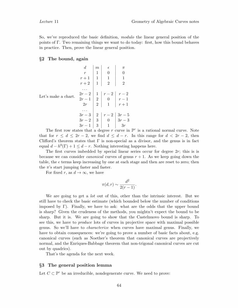
Lecture 11 Geometry of Algebraic Curves notes
So, we’ve reproduced the basic definition, modulo the linear general position of thepoints of Γ. Two remaining things we want to do today: first, how this bound behavesin practice. Then, prove the linear general position.
§2 The bound, again
Let’s make a chart.
d m ε πr 1 0 0
r + 1 1 1 1r + 2 1 2 2. . .
2r − 2 1 r − 2 r − 22r − 1 2 0 r − 1
2r 2 1 r + 1. . .
3r − 3 2 r − 2 3r − 53r − 2 3 0 3r − 33r − 1 3 1 3r
The first row states that a degree r curve in Pr is a rational normal curve. Notethat for r ≤ d ≤ 2r − 2, we find d ≤ d − r. In this range for d < 2r − 2, thenClifford’s theorem states that Γ is non-special as a divisor, and the genus is in factequal d− h0(Γ) + 1 ≤ d− r. Nothing interesting happens here.
The first curves imbedded by special linear series occur for degree 2r; this is isbecause we can consider canonical curves of genus r + 1. As we keep going down thetable, the ε terms keep increasing by one at each stage and then are reset to zero; thenthe π’s start jumping faster and faster.
For fixed r, as d→∞, we have
π(d, r) ∼ d2
2(r − 1).
We are going to get a lot out of this, other than the intrinsic interest. But westill have to check the basic estimate (which bounded below the number of conditionsimposed by Γ). Finally, we have to ask: what are the odds that the upper boundis sharp? Given the crudeness of the methods, you mightn’t expect the bound to besharp. But it is. We are going to show that the Castelnuovo bound is sharp. Tosee this, we have to produce lots of curves in projective space with maximal possiblegenus. So we’ll have to characterize when curves have maximal genus. Finally, wehave to obtain consequences: we’re going to prove a number of basic facts about, e.g.canonical curves (such as Noether’s theorem that canonical curves are projectivelynormal, and the Enriques-Babbage theorem that non-trigonal canonical curves are cutout by quadrics).
That’s the agenda for the next week.
§3 The general position lemma
Let C ⊂ Pr be an irreducible, nondegenerate curve. We need to prove:
64

Lecture 11 Geometry of Algebraic Curves notes
11.1 Theorem. For H a general hyperplane in Pr and Γ = C ∩H, then Γ is in lineargeneral position in H ' Pr−1.
11.2 Example. If r = 3, we have a space curve, and what we’re saying is that thegeneral plane section of a space curve has no three collinear points. Let’s prove this.We have a two-parameter family of secant lines, parametrized by pairs of points. Thefamily of secant lines is irreducible for this reason. A general secant line will meetthe curve again; it won’t be a trisecant. There is at most a one-dimensional familyof trisecants. Every trisecant lies only on a one-parameter family of planes, so thedimension of the space of planes containing a trisecant has dimension at most two. Sothere are planes that contain no trisecants. This means that there are planes H suchthat C ∩H contains no three collinear points.
Except showing that not every secant is a trisecant is not obvious at all. Castelnuovodid this with difficulty.
We’re going to look at this more generally. Again, let’s think of a curve C ⊂ P3.We have this curve and a plane H, general, which meets the curve in d distinct points.Let’s move the plane H around, taking care to avoid planes tangent to the curve. Solet’s move the plane in a 1-parameter family (parametrized by a real parameter t) Ht ofplanes transverse to the curve. As we move the plane, the set of points of intersectionHt ∩ C varies with the parameter t. As H wanders, we can try to follow each of thesepoints individually. Since t is a real parameter, we can do this in such a way to avoidthe tangent hyperplanes.
At the end of the day, we want H to wander in such a way to come back tothe original position. While the points have to collectively come back to the originalposition, they might get permuted. If {p1, . . . , pd} is the initial set of points, followingthe loop on H will induce a permutation in Sd. The claim is going to be that anypermutation can be induced—the monodromy group is full the symmetric group. Theconsequence is that there will be no distinguished subsets of these points H ∩ C. Itconsequently could not be the case that some triples are collinear and some triples andnoncollinear. This is going to easily imply the general position lemma.
§4 Monodromy
Let’s discuss this in general. This is a subject you can approach topologically, al-gebraically, or geometrically. Here’s the basic setup. We have a map φ : X → Y ofvarieties, smooth and projective. This is going to be a generically finite, dominant mor-phism. We want to say that there is a Zariski open subset U ⊂ Y such that φ−1(y) ⊂ Xconsists of reduced points, of cardinality equal to the degree. In fact, φ−1(U)→ U willbe a topological covering space.
So let’s look at this covering space φ−1(U)→ U . You have to go back to the earlydays when you were taught about covering spaces and fundamental groups. If p ∈ U ,then the fiber φ−1(p) is a finite set. The basic fact is that π1(U, p) acts on the fiberφ−1(p): the way it does so is to take a loop γ at p and a choice of point q in the fiber,take a unique lifting γ to φ−1(U) starting from q and ending at some other point, whichis γ.q.
65

Lecture 11 Geometry of Algebraic Curves notes
11.3 Definition. The induced subgroup of Sφ−1(p) which is the image of π1(U, p) iscalled the monodromy group.
This is not the same thing as the group of deck transformations. In general, thecovering space will have no deck transformations; to say that it does is to say that thecovering space is normal, or Galois.
OK, back to the varieties. We can associate the monodromy group associated to anydominant, generically finite map of varieties associated to the covering space genericallyinduced.
There are other ways of characterizing monodromy, as we said. Let’s do the al-gebraic version. We won’t justify this, as we won’t use it. But if you don’t like thecomplex topology, you can do it algebraically. Let C(Y ) ↪→ C(X) be the finite exten-sion of quotient fields. Take the Galois normalization L ⊃ C(X) (inside some algebraicclosure). The monodromy group, say G, is the Galois group of L/C(Y ).
It’s interesting—if you go back to the early history of Galois theory, what Ga-lois himself wrote was unreadable. You have to interpret very carefully, and nobodyunderstood what Galois was talking about until 1870 when Jordan wrote a book onthem. But half the examples are very familiar to us—number fields, and then the Ga-lois groups associated to extensions of function fields. This stuff was a part of Galoistheory that fell into disuse in the twentieth century.
Here’s the geometric description (partial). We will use it. Let’s make some obser-vations about the monodromy group G.
11.4 Proposition. G is transitive on the fiber if and only if the total space X isconnected. G is twice transitive (i.e. acts transitively on ordered pairs) if and only ifX×U X−∆ is connected. More generally, if Xr
U = X×U X×U · · ·×U X−∆ (r times)with all diagonals removed, so that
XrU = {(q, p1, . . . , pr) ∈ Xr : q ∈ U, φ(pi) = q, pi 6= pj} .
Then G is r-transitive if and only if XrU is connected.
Note that X×U X−∆ parametrizes distinct pairs of X which lie in the same fiber.This is really a direct consequence of the definitions. Note that Xr
U is a covering spaceof U .
We aren’t determining G, but we can at least say something about it.
§5 Proof of the general position lemma
We will prove something more general:Let C ⊂ Pr be a nondegenerate curve of degree d. Let C∗ ⊂ Pr∗ be the dual
hypersurface, which is the family of tangent (or non-transverse) hyperplanes. TakeU = Pr∗ −C∗ be the family of transverse hyperplanes (transverse to C). Let X be theset of pairs (H, p) such that p ∈ H ∩ C and H ∈ U . Consequently,
X ⊂ U × C
is a branched cover of U , of degree d (since every transverse intersection has d points).
66

Lecture 11 Geometry of Algebraic Curves notes
11.5 Theorem (Uniform position theorem). The monodromy group of X → U is thesymmetric group Sd.
This is true only in characteristic zero.
Proof. The first claim is that the monodromy group G is twice transitive. To see this,well, we have to consider X2
U = X ×U X − ∆: this is the set of triples (H, p, q) suchthat H is transverse to the curve, p 6= q, and p, q ∈ H ∩ C. We have to show that thisis irreducible; then we will get the double transitivity that we claimed. The proof withthis incidence correspondence, as always, is to look at it not as a covering of U but asa covering of C × C −∆, then it’s easy. Consider the map
X(2)U → C × C −∆, (H, p, q) 7→ (p, q).
The fibers of this map are (Zariski open subspaces of) projective spaces of dimensionr − 2, because once you fix two points, then we have a Pr−2 of projective spacescontaining the two points and we throw out tangent hyperplanes. So we have an
essentially Pr−2-bundle over an irreducible surface, which implies X(2)U is irreducible.
We’ve used: you have a dominant map, with irreducible fibers of the same dimen-sion. Then the total space is usually irreducible—not always. Well, it’s a bit subtle toprove this completely rigorously.
Anyway, the point is that one can deduce multiple transitivity by using this geo-metric argument.
Now, we claim that G contains a simple transposition. If we know that the groupG ⊂ Sd is twice transitive and contains a transposition, it must be the symmetric group(as it contains all transpositions). So, we have to show that it contains a transposition.We’ll do this by deliberately going to a point in C∗ ⊂ Pr∗, a tangent hyperplane,and look at the covering in a neighborhood of that point. The claim is that we canlet H wander in a neighborhood of that point and induce a simple transposition inmonodromy.
So let H0 be a hyperplane simply tangent to C. So H0∩C = 2p+d−2 other points .There’s contact of order two at one point and transversality everywhere else. (That’swhere characteristic zero enters: there are curves in characteristic p suchthat when a hyperplane is tangent, it is multiply tangent.) Choose a smallanalytic neighborhood V of H0, and we look at the family XV ∩U → V ∩ U . Theclaim is that the cover over this V ∩ U is going to consist of d− 2 copies of that sameneighborhood, all disjoint and all mapping isomorphically and one component which isstill connected but which maps 2-to-one onto the base. For this purpose, it makes senseto define the incidence correspondence for all hyperplanes, not just transverse ones. Sothe claim is that there are two sheets such that you can get from one to another bywandering the hyperplane.
Let’s say X = {(H, p) : p ∈ H ∩ C} which maps to Pr∗. Note that X is still smooth,and d− 2 of those connected components map isomorphically near H0; one maps two-to-one near H0. This will therefore induce a transposition in the monodromy.
N
67

Lecture 12 Geometry of Algebraic Curves notes
So, we’ve proved the uniform position theorem, and thus we’ve proved the basicestimate. By that very elementary lemma using hyperplanes, we get the bound onHilbert functions and we have completed the proof of Castelnuovo’s theorem.
This is stronger than the version in the book.
Lecture 1210/14
§1 General position lemma
Before we do anything else, let’s go over the last step in the general position lemma.Let C ⊂ Pr be a nondegenerate curve of degree d, and let H ⊂ Pr be a general
hyperplane. The claim is that H∩C is in linear general position. Last time, we showedthat if you vary H, and as you follow the points of intersection around, the monodromyinduced—the group of permutations of these points—is the full symmetric group. Fromthis we want to claim:
12.1 Proposition. No r points of H ∩ C are linearly dependent.
Proof. Let U = Pr∗ − C∗ be the family of transverse hyperplanes to the curve. Letus form the incidence correspondence X = {(H, p) : p ∈ H ∩ C} ⊂ U × C; this is ad-sheeted cover of U . We saw that the monodromy acts as the full symmetric group onthese d sheets. That is, the fiber product of X, any number of times, with itself (overU), with diagonals removed, will be an irreducible space. This is a consequence of themonodromy result, and in fact is true in nonzero characteristic as well.
OK, so let’s use this to prove the linear general position fact. Let Z be the setof pairs {(H, p1, . . . , pr) : p1, . . . , prlinearly independent, pi ∈ H} such that all the pi
are distinct and lie over the same point of U . This is a closed subvariety of X(r)U ,
the r-times fibered product X ×U × · · · ×U X with the diagonals removed. This Z is
nonempty, because we can choose linearly independent points on the curve. Since X(r)U
is irreducible, to say that Z ( X(r)U is to say that dimZ < dimX
(r)U . In particular, it
follows that the image of Z in U is a proper subvariety of U , because the map X(r)U → U
is a quasi-finite map.Things in U that are outside the image of Z are hyperplanes whose intersection
with the curve consist of linearly independent points. N
This is a common use of monodromy: we used the fact that the monodromy groupis the full symmetric group to conclude that certain varieties were irreducible.
Remark. We proved this for curves. It’s true for varieties in arbitrary dimension.If you have a k-dimensional variety X in Pr, then the intersection with a generalr − k-plane will give points in linear general position. You can deduce that from thestatement for curves (because a r−k-plane is an intersection of k hyperplanes, and theintersection of X with all but one of them is a curve). Or, one can imitate this proofdirectly.
So now we have completely proved the Castelnuovo bound.
68

Lecture 12 Geometry of Algebraic Curves notes
§2 Projective normality
Let’s recall the notion of projective normality.
12.2 Definition. Let C ⊂ Pr be a smooth curve. We say that C is projectivelynormal if, for every m, the hypersurfaces of degree m in Pr cut out a complete linearseries on C. In other words, if D is a divisor on C and D is linearly equivalent to mtimes the hyperplane divisor H (i.e. D ∼ mH), then D is the intersection of C with ahypersurface.
Or, the restriction map
H0(Pr,OPr(m))→ H0(OC(m))
is surjective. This is equivalent to saying that H1(IC,Pr(m)) = 0 for all m, where IC,Pr
is the ideal sheaf of C ⊂ Pr.
What does this mean geometrically? I can’t tell you that, but if you’re an algebraist—one of those people who read Atiyah-Macdonald and enjoyed the experience—here isan equivalent formulation (which is an exercise in Hartshorne).
12.3 Proposition. C is projectively normal if and only if the cone4 S ⊂ Pr+1 has theproperty that the local ring OS,p at the cone vertex p ∈ S is a Cohen-Macaulay ring.This, if and only if, S is a normal variety.
Let’s go back to Castelnuovo theory. Consider an irreducible, nondegenerate,smooth curve C ⊂ Pr. If we don’t assume C projectively normal, then we have asubspace H0(OPr(k))|C of H0(OC(k)) consisting of the image of H0(OPr(k)). This isa subseries; we call it Ek. If Ek is always the full linear series, then we have projectivenormality.
Last time, we proved a basic fact about the Em. We showed
dimEk − dimEk−1 ≥ min(d, k(r − 1) + 1).
For large values of n, we were able to bound below dimEn, and were able to useRiemann-Roch to bound above the genus g ≤ π(d, r).
The observation is that, if we have equality at the end, then we must have equalityat every stage. We must have not only
dimEk − dimEk−1 = min(d, k(r − 1) + 1),
but we must also have that each Ek is the full linear series (or we would have strictinequalities at some stage).
Thus:
12.4 Proposition. If g(C) = π(d, r), then C is projectively normal.
So extremal curves with respect to the Castelnuovo bound are projectively normal.
4I.e., imbed Pr ⊂ Pr+1, take a point outside it and draw lines from that point to C.
69

Lecture 12 Geometry of Algebraic Curves notes
12.5 Corollary. If C ⊂ Pg−1 is a canonical curve of genus g, then C is projectivelynormal.
This is because canonical curves are extremal.This means, in particular:
12.6 Corollary. Let C be non-hyeprelliptic. Every quadratic differential (section ofK2) is a quadratic polynomial in the holomorphic differentials. More generally, anypluricanonical differential on the curve is a polynomial in the holomorphic differentials.
This is interesting because quadratic differentials are useful in the geometry of, say,Teichmuller theory.
§3 Sharpness of the Castelnuovo bound
We’re now going to launch into an extended discussion of a topic whose relevance mayseem obscure. Remember what we said we had to do—we have now a bound g ≤ π(d, r)on the genus of a curve imbedded in projective space. That bound was based on a seriesof inequalities that we just wrote down, on the differences of the dimensions of the seriesOC(n). That seems very crude, but we saw that it is achieved, e.g. by points on arational normal curve. That suggests that if we want to look for curves that achievethis bound on the genus—our next goal—we need that for a general hyperplane sectionΓ of the curve, the Hilbert function of Γ is the minimum min(d, k(r− 1)) we gave. (Anexample of such a configuration Γ is any set of points on a rational normal curve.)
This means, once more, that if C is our curve, and Γ = C∩H is a general hyperplanesection, then we want Γ to lie on a rational normal curve. So what if C ⊂ P3, forinstance; then we’re saying that we need to look for configurations of points in the planewhich impose the smallest number of conditions on hypersurfaces. Here we would belooking for points lying on conics. So we might ask: can we take a curve in P3 suchthat the general hyperplane section consists of points lying on a conic? Sure; just takeC lying on a quadric. If C lies on a quadric, then the hyperplane section Γ will lie on aconic, and consequently the Hilbert function of Γ will be exactly min(d, k(r − 1) + 1).This does not, however, mean that curves on a quadric in P3 have maximal genus.
12.7 Example. If C lies on a smooth quadric Q ⊂ P3, and is of type (a, b), then wehave that a+ b = d (for d the degree) and g = (a− 1)(b− 1). The genus is maximizedwhen a, b as close to each other as possible, e.g. to d
2 . So a general curve on a smoothquadric won’t maximize the genus, though one can see that the best curve on a smoothquadric will achieve the bound.
If d = 2k, then one can check that g(C) can go up to (k − 1)2, and for d = 2k + 1,the genus can go up to k(k−1). These are in fact extremal curves. So the Castelnuovobound in P3 is sharp. When, however, one works with curves on a smooth which are ofthe form (a, b) for |a− b| > 1, then even though the hyperplane sections have the rightHilbert polynomials, projective normality fails (cf. the homework).
12.8 Example. Curves that lie on an irreducible cubic surface satisfy stronger boundson the genus (cf. the homework). The largest genus comes when you’re on a quadric.
70

Lecture 12 Geometry of Algebraic Curves notes
In general, we’re looking for curves C ⊂ Pr such that H ∩ C lies on a rationalnormal curve. We were able to achieve this in P3 by putting C on a quadric surface,which guarantees that the hyperplane section lies on a conic. We might ask ourselves:is there an analogous surface in Pr? Can we find a surface S ⊂ Pr such that H ∩ S isalways a rational normal curve? (One good suggestion is to take a cone on a rationalnormal curve; but we need something slightly different.) If we can find one such, andif we can understand what curves on this surface look like, then we might be able tohunt down the curves we want of maximal genus.
We’re going to take the next twenty and thirty minutes and talk about a moregeneral topic. At the end of the day, we’ll have a complete description of these surfaces.We won’t prove most of these assertions. If you want to see proofs, they’re in varioussources.
§4 Scrolls
We start with:
Question. What is the smallest possible degree of a variety X ⊂ Pr which is irre-ducible, nondegenerate, of dimension k?
For k = 0, there isn’t much to say.
12.9 Example. Let’s consider k = 1; we’re looking for nondegenerate curves in Pr ofsmallest degree. The answer is that the degree is at least r,
degC ≥ r.
and achieved for the rational normal curve. You can’t have anything with smallerdegree—if you have a curve in Pr, then r general points will span a hyperplane H; ifthe degree of the curve were < r, then C ⊂ H by Bezout, contradicting nondegeneracy.
12.10 Example. Let k = 2. We’re looking at surfaces in Pr. The claim is that anirreducible, nondegenerate surface S in Pr has the property that a general hyperplanesection will again be irreducible and nondegenerate. I.e., if H is a general hyperplane,then S ∩H will be a degS curve in Pr−1 which is irreducible and nondegenerate, so wefind that
degS = degS ∩H ≥ r − 1.
12.11 Example. In general, given a variety X ⊂ Pr of dimension k, we can useinduction and the above type of argument to see that
degX ≥ r − k + 1.
It turns out that this bound is achieved. If you don’t care about smoothness, thenyou can see that this bound is achieved by taking cones on a rational normal curverepeatedly.
Let’s now give an explicit construction of extremal surfaces in Pr, i.e. those ofdegree r − 1. Here’s the construction. In Pr, take a direct sum decomposition of the
71

Lecture 12 Geometry of Algebraic Curves notes
corresponding vector space; i.e., choose completementary linear spaces Pa,Pb ⊂ Pr.These span Pr and are disjoint. This implies that a + b + 1 = r. For instance, wecould take two skew lines in P3; a less simple example is a line and a 2-plane inP4. Next, choose a rational normal curve in each of these two subspaces; call theseCa ⊂ Pa, Cb ⊂ Pb. Choose an isomorphism of Ca with Cb (which we can do; both areisomorphic to P1). Call this isomorphism φ. Finally, take the surface S to be the unionof the lines joining p to φ(p) for p ∈ Ca, i.e.
S =⋃p∈Ca
p, φ(p).
For instance, we could draw a conic in P2 ⊂ P4, and connect corresponding points onthis conic to a line P1.
12.12 Definition. These are called rational normal (surface) scrolls. They aresometimes denoted Sa,b.
12.13 Proposition. These surfaces S just constructed have the minimal degree.
Proof. There are many ways to calculate the degree of this surface; we’ll do it ina concrete way. Choose a general hyperplane H containing one of those two linearsubspaces Pa,Pb. What is H ∩S? Well, obviously H ∩S will contain the curve Ca, butthere’s more. The hyperplane intersects Pb in a hyperplane in Pb, and that intersectionwill intersect the rational normal curve in d points. For each point p ∈ Cb that liesin H, the line through p and its image in Ca is also in H (because Ca ⊂ H). So, Hcontains the lines through the lines in Cb ∩H. It’s easy to see that there are no otherpoints in the intersection.
We find that H ∩ S is the union of Ca and lines through b points. The degree ofthis is a+ b; consequently by Bezout,
degS = a+ b.
N
To be careful, we should check that this calculation is legitimate, i.e. that theintersections occur with multiplicity one.
Remark. Suppose instead of choosing an isomorphism of the two curves, we chose aparametrization φ : P1 ' C, φ′ : P1 ' C ′. Then we could write S =
⋃t∈P1 φ(t)φ′(t).
That’s just another way of expressing it, but now we have an option not expressiblebefore; we could take one of a, b = 0 (in which case one of the φ, φ′ would be zero).We’d just get a cone over the nonconstant one of Ca, Cb. This, depending on yourpreferences, is also a scroll.
12.14 Theorem (Classical). The scrolls (including cones) are the surfaces of minimaldegree in Pr with one exception: that is, an irreducible, nondegenerate surface S ⊂ Prof degree r − 1 is either a scroll or the Veronese surface (isomorphic to P2) in P5.
We state this without proof. Note also that the Veronese surface contains no lines,and is very far from being a scroll. There is a generalization of this to more generalvarieties of minimal degree.
72

Lecture 12 Geometry of Algebraic Curves notes
Remark. The projective equivalence class of S = Sa,b only depends on (a, b), becausethe choices we made don’t really amount to much (a different choice, with a given (a, b),would be conjugate by automorphisms of projective space). Conversely, in a given Pr,no two of these Sa,b are projectively isomorphic; each is distinguished by the presenceof a curve of degree min(a, b) on it.
Here are two other things about the scrolls. These are both going to require somethought, but they’ll say something about them.
12.15 Proposition. Each surface scroll S is the projectivization5 P(O(a) ⊕ O(b)) ofthe vector bundle O(a)⊕O(b) on P1. The embedding is given by the tautological bundleon the projectivization.
One thing this result tells us which is worth remembering is that:
12.16 Corollary. Sa,b ' Sa′,b′ if and only if |a− b| = |a′ − b′|.
This is because tensoring a vector bundle by a line bundle doesn’t affect the pro-jectivization.
Next, let’s recall that a rational normal curve is a determinantal variety. In Pr, ifyou have a 2-by-r matrix of linear forms that looks like
A =
[L1 . . . LrM1 . . . Mr
]which are general, then the locus Φ of points p ∈ Pr such that this matrix A(p) has rankone, then this locus is a rational normal curve. The claim is that we can do somethingsimilar and construct the Sa,b. OK, let’s still take A a matrix,6 but one column short:
A =
[L1 . . . Lr−1
M1 . . . Mr−1
]and consider the locus of points p ∈ Pr where the rank is one. This is a scroll—we won’tjustify it, but it’s useful. For instance, what does it mean for a two-by-whatever matrixto have rank one? It means that the rows are independent. If we specified a specificrelation of linear independence, i.e. considered a pair [α, β] ∈ P1 and considered theequations αLi + βMi = 0, 1 ≤ i ≤ r − 1, then this is a line `α,β. As we vary [α, β], weget a family of lines parametrized by P1. This is in fact the scroll. (Determining thea, b in the scroll appears to be hard. The generic behavior is balanced.)
12.17 Example. Let X0, . . . , Xr be the linear coordinates on Pr. Consider the matrix[X0 X1 . . . Xa−1 Xa+1 . . . Xr−1
X1 X2 . . . Xa Xa+2 . . . Xr
];
this is of type (a, r − a+ 1).
5This is the post-Grothendieckian construction. That is, the projectivization of a vector space isthe set of hyperplanes in it.
6Technically, this should be 1-generic: this means no entry is zero, and no single row or columnoperation will make an entry zero.
73

Lecture 13 Geometry of Algebraic Curves notes
Ultimately, we are going to be talking about curves lying on these surfaces S. Sowe’ll need a similar description of curves on a scroll, just as we had a nice description(in terms of a pair of integers) of curves on a smooth quadric, that will enable us todetermine the genus. So, in other words, we need the intersection theory on a Sa,b.They’re not hard to derive, but now is not the time to do that. We’ll do that onMonday.
Let’s just say one more thing about these scrolls. We started out this whole dis-cussion with a simple question on varieties of minimal degree. Here’s another equallysimple question:
Question. Let X ⊂ Pr be a k-dimensional, irreducible, nondegenerate, variety ofdimension k. We have asked in the past how many hypersurfaces a curve lies on. So,what is the maximal number of (linearly independent) quadrics can X lie on?
Once we know an upper bound on the number of quadrics containing a variety, wemight also try to characterize the extremal ones.
In both cases, we are talking in some sense of the size of a variety. In some sense,the degree of a variety is a measure of its size; another is the number of hypersurfacesof some degree it lies on. We won’t prove this, but in fact:
12.18 Proposition. The maximal number of quadrics is(r+1−k
2
).
Proof. OK, let Y = H ∩X be the intersection of X with a general hyperplane H. Wehave a short exact sequence of sheaves (where I denotes the ideal sheaf)
0→ IX,Pr(1)→ IX,Pr(2)→ IY,Pr−1(2)→ 0
where the first thing is elements of the ideal sheaf vanishing on H, and we find that
H0(IX,Pr(2)) ↪→ H0(IY,Pr−1(2)).
By induction on the degree (and an analysis for points in P2), we can obtain the boundclaimed. N
Among surfaces, the extremal ones are the Veronese surface and the scrolls. Onecan see that scrolls lie on a lot of quadrics by representing them as a determinantalvariety, and looking at 2-by-2 minors.
Lecture 1310/17
§1 Motivation
From last time, let’s recall: C ⊂ Pr is a curve, smooth and irreducible and non-degenerate of degree d. We proved a bound
g(C) ≤ π(d, r) ≡(m
2
)(r − 1) +mε
74

Lecture 13 Geometry of Algebraic Curves notes
where d− 1 = m(r− 1) + ε such that 0 ≤ ε ≤ r− 2. We want to find curves of maximalgenus. To do this, (cf. the proof of the Castelnuovo bound) we want to maximize theHilbert function of the intersection C ∩ H with a generic hyperplane section H. Weknow that a configuration of points lying on a rational normal curve has a large Hilbertfunction, so we want to find C such that every hyperplane section lies on a rationalnormal curve.
Let d > 2r − 2. Note also that any extremal C is projectively normal. Thismeans that any quadric in H containing a hyperplane section H ∩C lifts to a quadriccontaining the curve C. The quadrics Q ⊂ H = Pr−1 containing the hyperplane sectionΓ = H ∩ C cut out a rational normal curve in Pr−1 (because the degree is > 2r − 2),so the quadrics in Pr containing C cut out a surface whose hyperplane section is thatrational normal curve.
So we’re looking for curves on a surface S of minimal degree. This will be, withone intersection, a scroll.
§2 Scrolls again
Now we need to describe the geometry of scrolls and curves on scrolls. To construct ascroll, depending on parameters a ≤ b ∈ Z, we take Pr, two complementary subspacesPa,Pb, and draw rational curves Ca ⊂ Pa, Cb ⊂ Pb, choose an isomorphism between thetwo Ca ' Cb, and draw lines between corresponding points. One can show that one infact gets a smooth surface Sa,b, whose degree must be a+ b.
13.1 Definition. The curve Ca ⊂ Sa,b is called the directrix.
Let us describe a few facts.If you take a scroll, and project from a line on the ruling, then you project to Pr−2:
lines map to lines, Ca maps to a rational normal curve of degree a − 1, and Cb mapsto a rational normal curve of degree b− 1. So, if you project from a line of the ruling,you get an isomorphism of Sa,b with Sa−1,b−1. If you projected from a point of Ca orCb, then you would only get a rational map. Projecting from a Cartier divisor gives aregular map.
Consequently, Sa,a ' S1,1 ' P1 × P1, because S1,1 is a quadric surface. Moreover,Sa,a+1 is isomorphic to a cubic scroll in P4. This is, moreover, isomorphic to the blow-up of P2 at a point p. Why is this? If you blow up a point in P2, then you replacea point in P2 with an exceptional divisor, and the lines passing through that pointbecome disjoint. If you choose a second line in the plane, not passing through theblown up point, it’s exactly the same picture: it follows that the blown up surface isswept out by lines joining the two, disjoint. More formally, consider the space of conicsin P2 through the point p; this gives a rational map from P2 → P4, which becomesregular on the blow-up, and imbeds the blow-up in P4.
§3 Intersection numbers
OK, let’s go back to where we were. We have a scroll Sa,b obtained by joining corre-sponding points on curves in complementary projective spaces. We can think of this
75

Lecture 13 Geometry of Algebraic Curves notes
as swept out by lines, and it’s a bundle over P1. The fibers are these lines. Let H bea hyperplane divisor in Sa,b.
We now want to understand the Picard group of Sa,b and the intersection pairing.This is a straightforward exercise. Here is an outline:
13.2 Proposition. Pic(Sa,b) is freely generated by the classes f (the class of a fiber,i.e. the lines in the ruling) and h (the class of a hyperplane H).
Proof. In fact, we just have to make the following observation. If we take Sa,b andremove a fiber and remove a hyperplane section of S, what we have left is a bundleof affine lines over an affine space—so it’s A2, which has trivial Picard group. Thusthe Picard group must be (by the standard exact sequence, or because the triviality ofPic(A2) means that divisors can be “pushed” onto the union of h and f) generated byh and f . Consequently, the rank of the Picard group is at most 2.
More generally, if you’re familiar with projective bundles, you can appeal to ageneral fact about the Picard groups of them.
OK, let’s compute intersection products. We will use these numbers below.The intersection h.h is the intersection of two hyperplanes, which is the degree of thesurface r − 1. We also easily get h.f = 1 and f.f = 0 (two fibers are disjoint, and ahyperplane class hits f , which is a line, once). This also shows that h, f are linearlyindependent in the Picard group, which must thus be Z2.
N
We could also compute the classes of Ca, Cb in Sa,b. A general hyperplane Hcontaining Ca intersects Cb in a total of b points and consequently Ca ∩H will be theunion Ca and b lines of the ruling. So the divisor of Ca is h − bf and that of Cb ish− af .
Note that the self-intersection of Ca is a − b ≤ 0, while Cb.Cb = b − a ≤ 0. Thetwo curves really behave differently from each other. In fact, Ca is the unique curve ofdegree ≤ a (other than the lines) on this surface if a < b.
Finally, we need to know the canonical class of Sa,b. This is a natural thing to askwhen you work out the Picard group. There are probably better abstract ways of doingthis. For instance, you could write down an explicit 2-form by writing down equationsand then count zeros and poles. But that’s too much like work, and “cheat” (it’s notcheating; it’s legitimate)
KS = αh+ βf
for some α, β ∈ Z. How can we find α, β?Let’s apply adjunction to the curves we know about on the surface. Let’s apply it
to the fiber f itself, which is a fiber: we know that f is a line, which has genus zero.So the canonical class of f has degree −2. But the canonical class of f is
(KS + f)|f ,
so the degree is (αh+ βf).f = α. It follows that α = −2. Now, we can do it one moretime to figure out β; let’s take a hyperplane class h.
The hyperplane section is a rational normal curve. So we do this again, and have
−2 = (KS + h).h = (αh+ βf).h+ r − 1 = β − (r − 1).
76

Lecture 13 Geometry of Algebraic Curves notes
Thus β = r − 3.We find:
13.3 Proposition. The canonical series KS = −2h+ (r − 3)f .
That’s why this basis for the Picard group is nice; note that the answer doesn’tdepend on a, b.
Remark. You should check that this is consistent with applying adjunction to Ca, Cband the self-intersection of these curves. You should immediately check this in the casewhere r = 3, where the scroll is a quadric is P3, and where adjunction in P3 gives thecanonical class of the scroll, which we found earlier to be −2h. This is just what theabove analysis gave.
Now that we know the canonical class and the intersection products, we can sayexactly what the genus of a curve on the scroll is. Let C ⊂ Sa,b ⊂ Pr is a scroll. As adivisor in S, we can write C = αh + βf ; this means that α is the number of times Cmeets a line of the ruling. What we’d like to is to compute the degree and genus of Cvia α, β.
1. The degree of C in Pr is the intersection of C = αh + βf with the hyperplaneclass h, which is α + (r − 1)β by the earlier basis and the intersection numberscomputed.
2. The genus of C can be found via adjunction. Namely, we can get it from
C.(KS+C) = (αh+βf).((α−2)h+(β+r−3)f) = α(α−2)(r−1)+β(α−2)+α(β+r−3).
This can be simplified to
α(α− 1)(r − 1) + 2αβ − 2α− 2β.
The conclusion is that
g(C) =
(α
2
)(r − 1) + (α− 1)(β − 1).
Note that we’re using a different basis for the Picard group that we would use for thequadric in P3.
OK, now we want to find extremal curves, i.e. choose α, β appropriately to maximizethe genus.7 For a fixed value of the degree, we want to find the maximal value of thegenus by the above answer. You can assign it to your calculus class—you’ll see whatyou get. We’ll just state the answer.
Answer: To maximize g, take
α = m+ 1, β = ε− r + 2.
The degree in this case is m(r − 1) + ε+ 1, which is what you want. The genus worksout to be
(m2
)(r − 1) + mε. This in fact gives the right answer; we saw this was the
upper bound. (If ε = 1, we can also take α = m,β = 1.)Is it clear that any such divisor class is represented by a smooth curve on a scroll?
Let’s answer this question. Here’s a little lemma, worth pointing out.
7We have to show that a given divisor class contains a smooth curve, though.
77

Lecture 13 Geometry of Algebraic Curves notes
13.4 Lemma. The class αh+ βf on Sa,b is represented by a smooth (not necessarilyirreducible) curve on the Sa,b if α = 0, β ≥ 0 (this is a collection of lines on the curve)or if α > 0, and β ≥ −αa.
The only if case is more complicated and has more cases.
Proof. Use Bertini’s theorem. This states if you have a linear series of divisors withoutbase points, then the general member of that linear series is smooth. That applies inthis case, because αh + βf = α(Cb) + (β + aα)f (this is because Cb = h − af). Ifthe second term is nonnegative, one can check that the linear series has no basepoints;for this one needs to check that Cb moves in a linear series without basepoints. Thusamong the curves in this class are smooth curves. N
To show that you can get these curves to be irreducible, you need a further argumentwith intersection numbers: if you had two curves whose classes added up to αh + βfin this way, they would have to intersect, which can’t happen.
Bertini’s theorem is frequently used to show that a family has smooth divisor classesby exhibiting non-smooth elements of a divisor class.
Remark. In case r = 5, and d is even, then we can take C to lie on a Veronese surface.The Picard group of a Veronese surface (which is isomorphic to P2 is rank one) and C isthe image of a plane curve under the Veronese imbedding. So you can check that takingimages under the Veronese of plane curves can also be used to satisfy the Castelnuovobound. We won’t do this.
Now what? We’ve established the maximum possible genus of a curve in Pr, whichis cool, but we want to know more. What comes next is a really remarkable theorem.It gives a sort of converse. What we’re going to prove is, you get in one of these ways,all curves of maximal genus.
We proved, first of all, an inequality on the Hilbert function of a number of pointsin linear general position in Pr. By applying that to hyperplane sections, we estimatedH0(C,OC(m)) from below for a curve C in Pr. We saw that the inequality on theHilbert function could be satisfied by points on a rational normal curve. Now we aregoing to state something much stronger. We’ll give an indication of the proof, and doit properly on Wednesday.
13.5 Theorem (Castelnuovo’s lemma). If Γ ⊂ Pn is a configuration of d ≥ 2n + 3points in linear general position, which impose only 2n + 1 conditions on quadrics,8
then Γ lies on a rational normal curve.
We’ll go through the proof on Wednesday, and describe why it’s so important.Basically, it’s going to tell us that a curve of maximal genus (and degree at least2n + 3) lies on a rational normal scroll or Veronese surface, because the only way toget the hyperplane sections to lie on a rational normal curve is (as we saw earlier—inJefferson) is to have the curve lie on a surface.
8We saw that the number of conditions imposed on quadrics is at least the minimum of the degreeand 2n+ 1, and here that minimum is 2n+ 1.
78

Lecture 14 Geometry of Algebraic Curves notes
The idea of the proof will be a beautiful, old-fashioned idea called the Steinerconstruction. Let’s say we have Λ1, . . . ,Λn ' Pn−2, codimension two subspaces inPn. Let
{H it
}t∈P1 be the pencil of hyperplanes containing the plane Λi. For instance,
in case n = 2, we’d be looking at pencils of lines containing points. Consider theintersection of the hyperplanes in each of these pencils, i.e.
H1t ∩ · · · ∩Hn
t
of the n hyperplanes parametrized by the same parameter. In general, this intersectionshould be a point. Let’s suppose this is true; it is true generally. Then, for each valueof t, we can take the union of these points
⋃tH
1t ∩ · · · ∩Hn
t , which will be a rationalnormal curve in Pn. (Exercise.)
In fact, we can give a slightly stronger statement. Instead of taking n pencils ofhyperplanes, let’s say we take l < n pencils of hyperplanes H i
t for 1 ≤ i ≤ l andt ∈ P1. Again, we consider the variety swept out by the intersections
⋂iH
it over all t;
we assume that these intersections are dimension n− l. So we get a variety swept outby Pn−l’s, which in fact will be a rational normal scroll of dimension n− l+ 1. This isnot obvious.
Proof. Observe that the map φ : P1 → Gr(n− l, n) sending t 7→⋂iH
it is given by the
wedge product of the linear forms P1 → Gr(n − 1, n) that describe each H it . So this
map φ has degree l (when the Grassmannian is imbedded in some projective space).In general, when you have a map to the Grassmannian, the variety swept out is equalto the degree of this map. So it follows that the degree of the variety X swept out bythese intersections is degree l, and consequently one sees that it has minimal degreeand must be a scroll (being swept out by linear spaces, it’s not a Veronese surface). N
This is another old-fashioned construction of the scroll, which we’ll use to proveCastelnuovo’s lemma.
Lecture 1410/19
Last time, we were about to embark upon a project to completely characterize curves ofmaximal genus. We had derived Castelnuovo’s inequality, which gives an upper boundfor the genus of a curve in projective space. By doing intersection theory on scrolls,we showed that the bound was sharp. Now we want to do something even stronger—we want to characterize these extremal curves. The key element was this lemma ofCastelnuovo, which we’re about to prove.
§1 A basic lemma
We first need:If Λ1, . . . ,Λk is a collection of Pn−2’s in Pn (a bunch of codimension two planes, e.g.
points in P2 or lines in P3) where k ≤ n, consider the pencil of hyperplanes containing
79

Lecture 14 Geometry of Algebraic Curves notes
each of these hyperplanes containing them.9 Let{H it
}t∈P1 be the pencil of hyperplanes
containing Λi. For each value of t, consider the intersection H1t ∩ · · ·∩Hk
t ; assume thatthis is a transverse intersection always, so the intersection is a Pn−k at all times.
Consider the union X =⋃t∈P1 H1
t ∩ · · · ∩Hkt . This should sweep out some variety
X.
14.1 Example. If you have two lines in P3, say `1, `2, then we’re taking the set ofplanes containing each of the two lines, pairwise intersecting them, and taking thesurface swept out by these intersections. But this corresponds to joining correspondingpoints on the two lines, so gives a scroll.
14.2 Lemma. In general, X is always a rational normal scroll.
Proof. Consider the map φ : P1 → G(n− k, k) (the Grassmannian in projective space)sending t 7→ H1
t ∩ · · · ∩ Hkt . What does this map look like? If we dualize and think
of it as G(k − 1, n∗) of k − 1-planes in the dual space, then each pencil of hyperplanesis given by a linear form varying linearly with t. So H i
t = V (`it) for `it a linear formvarying linearly with t. Then the map φ sends t 7→ V (`t1 ∧ · · · ∧ `tk); this is thus a curveof degree k under the Plucker embedding. That means (we’ll just quote this) that thecorresponding X has degree k in Pn, and since this is minimality, we get that X is ascroll. N
We’re invoking way too much here. Let’s say it alternatively. If we write H it as the
zero locus of a linear combination H it = V (t0L
i + t1Mi) for Li,M i linear forms, then⋂
iHit is thus the locus where the matrix[
L1 . . . LkM1 . . . Mk
]is such that t0 times the first row plus t1 times the first row vanishes, and as t varies,this sweeps out a scroll (where this matrix has rank ≤ 1).
We need another little lemma.
14.3 Lemma. In Pn, if p1, . . . , pn+3 are points in linear general position, then p1, . . . , pn+3
lie on a rational normal curve.
For instance, five points in P2, no three of which are collinear, lie on a smooth conic.In P3, we find that six points, no four of which lie in a plane, lie on a twisted cubic.We want to use the above construction to give such examples.
Proof. Consider the first n points p1, . . . , pn. Take the planes in the above constructionto be the Pn−2’s spanned by n− 1 of the above points. So,
Λi = p1, . . . , pi, . . . , pn
so this is the span of p1, . . . , pi−1, pi+1, . . . , pn. Then, choose the parametrization ofeach pencil H i
t containing Λi such that the element of this pencil that passes throughpn+1 has t = 0, and similarly for the others. That is, and more precisely, we require
pn+1 ∈ H i0, pn+2 ∈ H i
∞, pn+3 ∈ H i1.
9Because they’re codimension two, each lies on a pencil of hyperplanes.
80

Lecture 14 Geometry of Algebraic Curves notes
We can do this by reparametrizing.Now, if we take X =
⋃t∈P1
⋂iH
it , then this contains p1—that’s because p1 will lie
on Λ2, . . . ,Λn and thus on all the H2t , . . . ,H
nt , and it will lie on some H1
t . So p1 ∈ X.Similarly all the pi ∈ X for 1 ≤ i ≤ n, and the last three do as well by the aboveconstruction (taking t = 0, 1,∞). But by the above lemma, this X is a rational normalcurve.
This is called Steiner’s construction. N
§2 Castelnuovo’s lemma
Now let’s restate and prove Castelnuovo’s lemma.
14.4 Theorem (Castelnuovo). Consider Γ = {p1, . . . , pd} ⊂ Pn. Let’s make the fol-lowing assumptions:
1. Γ is in linear general position.
2. d ≥ 2n+ 3.
If hΓ(2) = 2n+ 1,10 then Γ is contained in a rational normal curve.
By way of an example, let’s see why this is necessary.
14.5 Example. Take n = 3. So we have P3, and let’s say you have eight points in lineargeneral position. Can they impose seven conditions on quadrics? Since the space ofquadrics is ten-dimensional, this is to say that the eight points lie on a net of quadrics.The answer is yes—just take three quadrics, and pick the intersection. In other words,the transverse intersection of three quadrics will be eight points, generically in lineargeneral position, which will impose only seven conditions. They don’t lie on a rationalnormal curve because then the rational normal curve would lie on each of the quadrics.
14.6 Example. If we have nine points in P3, and they lie on three quadrics, then byBezout the intersection of three quadrics must be positive-dimensional. Ultimately onesees that the intersection is a twisted cubic (after some work).
Proof. Again, let Λi be p1, . . . , pi, . . . , pn be the span of the first n points with the ithomitted. Choose the parametrizations of the pencils H i
t (for t ∈ P1) of hyperplanescontaining Λi such that
pn+1 ∈ H i0, pn+2 ∈ H i
∞, pn+3 ∈ H i1, ∀i.
We know that the rational normal curveX swept out by⋂iH
it containing these contains
p1, . . . , pn+3, as in the earlier argument today. We want to see that this contains themall.
OK, take Λ = pn+4, . . . , p2n+2. Take again {Ht} as the pencil of hyperplanes con-taining Γ. Again, we normalize so that
pn+1 ∈ H0, pn+2 ∈ H∞, pn+3 ∈ H1.
10This is the Hilbert function.
81

Lecture 14 Geometry of Algebraic Curves notes
Let Qi =⋃t∈P1 H i
t ∩Ht. This is a union of codimension two planes, and it’s varyingwith one degree of freedom. It has codimension one. The claim is that Qi is a quadric;in fact, it’s a scroll of codimension one, so it’s a quadric hypersurface by the earlierlemma today. It contains a bunch of points. It contains the points in Λi, so it containsp1, . . . , pi, . . . , pn, and it also contains pn+1, pn+2, pn+3, and also pn+4, . . . , p2n+2. If wecount these up, we get 2n+ 1 points of the configuration Γ. If any 2n+ 1 points of Γimpose independent conditions on quadrics, then any quadric containing 2n+ 1 pointsof Γ must contain Γ.
Now we’re done, because all the remaining points have to match up. Well, thatsays in turn that for all points from 2n + 3 onto d, that is for p among p2n+3, . . . , pdwe find that the value of t such that H i
t contains p is equal to the value of t such thatHt contains p. (That’s because all the remaining points lie on the quadric Qi.) Thismeans in particular that the value of t such that H i
t contains p is also the same as thevalue of t such that Hj
t contains p. That implies in turn that p2n+3, . . . , pd all lie on X.We still have to check that pn+4, . . . , p2n+2 lie on X; by construction they lie on
each quadric, but they don’t obviously match up. However, since there’s at least morepoint, you can swap it and use the same argument: we know by know that X containsp1, . . . , pn+3 and there is a unique rational normal curve containing those. You canswap points to get the same rational curve. N
(Being tired, I didn’t really follow this, and this argument may not be faithfullywritten down.)
§3 Equality in the Castelnuovo bound
Let C ⊂ Pr be a nondegenerate curve of degree d. Then g(C) ≤ π(d, r). If equalityholds there, i.e. g(C) = π(d, r) and d ≥ 2r + 1, then the generic hyperplane sectionΓ = C ∩ H must lie on a rational normal curve in Pr−1 by the previous lemma ofCastelnuovo. The intersection of quadrics in Pr−1 containing Γ must be that rationalnormal curve, and since those quadrics in Pr−1 lift to quadrics in Pr containing thecurve (by projective normality).
So we have used two facts:
1. The intersection of quadrics in Pr−1 containing Γ is this rational normal curve Bin Pr−1 that the points lie on.
2. The intersection of quadrics in Pr containing C must be a surface of minimaldegree, which is thus either a Veronese surface or a scroll.
Anyway, we have seen that curves on a scroll or on a Veronese surface can achievethis bound.
We now have an exact list of curves of maximal genus.
14.7 Theorem. A curve in Pr of degree d meeting the Castelnuovo bound and thatsatisfies d ≥ 2r + 1 lies on a Veronese surface or a scroll.
Remark. A canonical curve does not satisfy d ≥ 2r + 1.
82

Lecture 14 Geometry of Algebraic Curves notes
Let’s draw one interesting consequence. If you take the quadrics containing such acurve, you’ll get a scroll. Let’s ask the same question with a canonical curve.
Take a canonical curve C ⊂ Pr with g = r − 1 and d = 2g − 2 − 2r. The abovedoesn’t apply, but we might consider the intersection over quadrics X =
⋂C⊂Q⊂Pr Q;
this is an intersection of quadrics which contains C. Suppose X contains one morepoint p /∈ C.
Take a general hyperplane H containing that point p. Consider the correspondingplane section H ∩ C: there are 2r points of intersection p1, . . . , p2r. You’ll see thatin this case, if you review the proof of the uniform position lemma, the points of ahyperplane section of a curve together with the point p, are in linear general position.That is, p1, . . . , p2r, p are in linear general position. That’s not obvious. The first 2rare in linear general position by the general monodromy argument. Then you have toargue that p together with any 2r−1 points among p1, . . . , p2r will still give you a largemonodromy group. That’s a crucial observation.
Now, every quadric in projective space containing the curve C contains p. It followsthat any quadric in H containing p1, . . . , p2r contains p. It follows that {p1, . . . , p2r, p}impose only 2r − 1 conditions on quadrics. We have enough points that Castelnuovotells us that p1, . . . , p2r, p all lie on a rational normal curve. Now the same logic goesthrough as before. It follows that the intersection of all quadrics in projective space issuch that the general hyperplane section is a rational normal curve, by the same logic.So this intersection of quadrics, if it’s not C, is a scroll or Veronese surface.
We have proved:
14.8 Proposition. A canonical curve lies on a scroll or a Veronese surface, or it’sthe intersection of quadrics.
One can see that the class of the curve is 3h− (r − 3)f .
Remark. This means that the canonical curve will meet the lines of the ruling threetimes. In other words, the lines of the ruling will cut out a g1
3 on the curve. Thisimplies that a canonical curve lying on a scroll is trigonal. Conversely, if we startwith a trigonal curve and look at the canonical model, the geometric Riemann-Rochtheorem shows that there are triples of collinear points lying on the points. Everyquadric containing the canonical model must contain the line through these points.Then in that case the canonical model lies on the scroll and the lines of the ruling cutout the g1
3.If C lies on a Veronese surface and is a canonical curve, then C must be the image
of a smooth plane quintic.
We find:
14.9 Theorem (Enriques). If C ⊂ Pg−1 is a canonical curve, then C is cut out byquadrics containing it unless C is either trigonal or C is a plane quintic.
This is saying something genuinely interesting about the geometry of canonicalcurves. Once you get beyond degree 2r in Castelnuovo theory, the curves you’re lookingat of maximal genus are very special. This argument, as it stands, tells us nothingexcept about curves about that single maximum genus. It says nothing about curves of
83
Lecture 15 Geometry of Algebraic Curves notes
genus one less at the maximum. The homework assignment will hint at these questions.It’s interesting to ask how much of this analysis applies to curves of relatively high genus.
We have a sequence of logical steps: we’re looking for a curve of largest possiblegenus. A curve of higher genus has a smaller Hilbert polynomial, so it lies on morehypersurfaces of large degree. To find curves of largest degree, Castelnuovo foundcollections of points with minimal Hilbert function. These were points on rationalnormal curves; this is reasonable, because a rational normal curve is a curve minimizingthe Hilbert function.
Now, suppose you want to look for configurations of points that have a small, butnot really small, Hilbert function—a little larger than the minimum possible Hilbertfunction. We saw that if Γ is in linear general position, then hΓ(m) ≥ min(d,m(r−1)+1) for d the degree. What’s another set of points, not lying on a rational normal curve,that is close to this? One example: points lying on an elliptic curve. Or a projectionof a rational normal curve. It turns out the elliptic curve wins.
If Γ is contained in an elliptic normal curve, then
hΓ(m) ∼ min(d,mr).
If we start with a curve whose Hilbert function is this, we can derive in the same way abunch of inequalities on the genus as before, the bound on π(d, r) is strikingly different.
We find in this case that the genus g(C) ≤ π1(d, r) ∼ d2
2r . So, in the range betweend2
2r−2 (the Castelnuovo bound) and this d2
2r , we’ll be able to conclude that they have tolie on scrolls.
Conjecturally, curves of large genus should lie on surfaces of small degree.
Lecture 1510/21
§1 Introduction
We want to talk today about extensions of Castelnuovo theory. Today, we’ll talk aboutsomething which is still being researched. We won’t use it in the rest of the course,so if you’re not looking for an interesting problem, just treat this as an occasion toget acquainted with an interesting problem, or just ignore it altogether. You have mypermission.
You have to have a nineteenth-century mindset for this. If someone asked youtoday to classify curves, most people would answer the question by saying that “smoothprojective curves have one discrete invariant (the genus), and within each genus a singleirreducible family of dimension 3g−3.” If you wanted to say more, you would describethe space Mg parametrizing curves. In the nineteenth century, abstract curves weren’tdefined, so if you asked someone like Castelnuovo how to classify all curves, they wouldinterpret the word “curve” as a subset of Pn for some n. In this case there are twodiscrete numerical invariants: the genus and the degree. So the first question youwould ask is the analog of the statement that all genera occur—which degrees andgenera occur? Castelnuovo’s theorem, which we’ve gone through and proved, is thefirst step towards answering that: it gives a sharp upper bound.
84

Lecture 15 Geometry of Algebraic Curves notes
But it doesn’t answer the question. We now know what the maximum genus is, butwe don’t know about genera between zero and the maximal bound. The proposal thatI’m going to make is to investigate this by going back to Castelnuovo’s argument andseeing how it might be modified to address curves of large genus.
In the course of proving Castelnuovo’s theorem, we derived a lower bound on theHilbert function configuration of points in a hyperplane section. To do this, we usedthe fact that these hyperplane sections had points in linear general position. But thisfact was a consequence of something stronger. We said that if C ⊂ Pr was a curve,then when you look the set of hyperplanes transverse to C, the monodromy of thesepoints as you vary the hyperplane gives the full symmetric group. But you can saymore.
Let H be a general hyperplane. Consider the monodromy on H∩C = Γ as H varies.This is the symmetric group on d letters (for d the degree). This implies that for allΓ′,Γ′′ ⊂ Γ of the same cardinality and for all m, the Hilbert function hΓ′(m) = hΓ(m).In other words, you cannot distinguish between subsets of Γ of the same cardinality.Remember how we set this up—we looked at
X = {(H, p) : p ∈ H ∩ C} ⊂ U × C
where U is the open subset in Pr∗ consisting of transverse hyperplanes, and argued that
the fiber product X(k)U was irreducible. That implies that the monodromy is k times
transitive. Inside X(k)U there is an open subset where the number of conditions is maxi-
mal. For a general point in U , all the k tuples of points in the corresponding hyperplaneimpose the same numbers of conditions. This again follows from irreducibility.
15.1 Proposition (Uniform position). For any general hyperplane H, and two Γ′,Γ′′ ⊂Γ = C ∩H of the same cardinality k and for all m, we have hΓ′(m) = hΓ′′(m),∀m.
So you can’t distinguish between subsets of the same cardinality using intrinsicinvariants. We are going to use this strengthening of the linear general position lemmatoday.
§2 Castelnuovo’s argument in the second case
Castelnuovo started this off by arguing that if a configuration of d points Γ ⊂ Pn is inlinear general position, then
hΓ(m) ≥ h0(m) ≡ min(d,mn+ 1).
This is achieved by taking points on a rational normal curve, where in fact: if Γ ⊂ Bfor B a rational normal curve, then hB(m) = mn + 1 for all m. When d is large,then any hypersurface of degree m which contains Γ will contain B and the number ofconditions imposed by Γ and by B will be the same.
So we have this “minimal Hilbert function” which is achieved by points on a rationalnormal curve. Last time, we observed that h0(m) was the smallest possible Hilbertfunction of such a configuration of d points, under linear general position. Now let’sassume uniform position, and ask what the second smallest possibility for the Hilbertfunction.
85
Lecture 15 Geometry of Algebraic Curves notes
The point was h0(m) was the minimum of d and mn + 1, where mn + 1 was theHilbert function of a curve that was as small as possible: the rational normal curve.So we were looking at points that lie on curves of small Hilbert function. What’s thesecond smallest candidate? The claim is that we can do second-best by taking the setΓ to lie on a linearly normal elliptic curve.
Recall:
15.2 Definition. A curve C ⊂ Pr is linearly normal if H0(OPr(1))→ H0(OC(1)) issurjective. This is equivalent to saying that the imbedding C ↪→ Pr does not factor asan imbedding C ↪→ Pr+1 followed by a projection, or that the linear system cut out byhyperplanes is complete.
When the degree of the curve is small (less than 2r), you checked on the homeworkthat linear normality implies projective normality.
Let’s make the following claim:
The second smallest (irreducible, non-degenerate) curve in Pn is an elliptic(linearly) normal curve of degree n+1. In other words, one takes an ellipticcurve B, an ample line bundle L of degree n + 1, and imbeds E in Pn viathe complete linear series L.
In this case, the Hilbert function of B is
h0(OB(Lm)) = m(n+ 1)
by Riemann-Roch. Notice that the Hilbert function of a rational normal curve is justmn+ 1; the difference here is a shift in the degree, while the genus has jumped.
Another candidate would be to consider a rational (non-normal) curve of degreen+ 1 in Pn, but the Hilbert function would be a little more because the genus is zero.
Let’s state the result more formally:
15.3 Proposition. Among all irreducible non-degenerate curves B ⊂ Pn, the linearlynormal elliptic curve of degree n+ 1 has the second-smallest Hilbert function.
The proof is left as an exercise.Now suppose Γ ⊂ B is a finite set of cardinality d, in uniform position. Then
hΓ(m) =
hB(n) = m(n+ 1) if d > m(n+ 1), by Bezout
d if d < m(n+ 1)
d− 1 if d = m(n+ 1)
In the latter case, the points impose independent conditions. Note that there is aslight gap in here. It’s possible that the points Γ could be exactly the intersection ofa hypersurface of degree m with the elliptic normal curve. We won’t write out all thedetails. This is exactly what is described in part III of the Montreal books.
Remark. It is nearly true that points with the Hilbert function as above lie on anelliptic curve.
86

Lecture 15 Geometry of Algebraic Curves notes
Let’s call this function h1(m). We said that h0(m) was the smallest possible Hilbertfunction; h1(m) is the second-smallest. Now recall how Castelnuovo proceeded. He gota bunch of inequalities
h0(OC(k))− h0(OC(k − 1)) ≥ h0(k)
which he added up for varying k. This he used to bound the genus of C using Riemann-Roch.
So we now have a second-smallest Hilbert function. What we now want to concludeis, referring back to the picture of C ⊂ Pr and Γ the points of a general hyperplanesection, then if Γ doesn’t lie on a rational normal curve, then
hΓ ≥ h1.
(I’m not sure that we proved this.) We can, in this same way, inequalities
h0(OC(k))− h0(OC(k − 1)) ≥ h1(k),
which gives better lower bounds on the Hilbert function of C, and thus better upperbounds the genus. The significant improvement between h0 and h1 gives a much betterupper bound for the genus. We won’t write this all out, so we’ll just state:
15.4 Theorem. For a curve C whose general hyperplane section doesn’t lie on a ra-tional normal curve,
g(C) ≤ π1(d, r) ∼ d2
2r
Contrapositively, if the genus is bigger than π1(d, r), then the hyperplane sectionlies on rational normal curves, and we can in fact conclude:
15.5 Proposition. If g(C) > π1(d, r), then C lies on a rational normal scroll.
The point is that there aren’t that many genera on a rational normal scroll, becausethe Picard group is so simple. For instance, there was a homework problem on thissort of thing. If S is a cubic surface in P3, then any C of genus g(C) > π1(d, r) ∼ d2
6must lie on a quadric with balanced type.
This was first observed by Halphen: he analyzed curves lying on cubic surfaces,then quartic surfaces, etc. He gave a complete answer to the answer of what (d, g) maybe in P3, and got a huge prize for it—though it was later discovered his argument hada serious flaw. The standards of proof have shifted since his work.
§3 Converses
We’d now like to talk briefly about what’s next. There is an analog of Castelnuovo’slemma in this setting, and it states:
15.6 Proposition (Fano). If Γ ⊂ Pn is a configuration of points in uniform position,consisting of d ≥ 2n+ 5 points, if Γ imposes the second smallest number of conditionson quadrics—that is, if hΓ(2) = 2n+ 2—then Γ lies on an elliptic normal curve.
87

Lecture 15 Geometry of Algebraic Curves notes
This is proved in the Montreal notes. Where is this all leading? The generalconjecture is going to be that if we have a configuration of points that imposes fewindependent conditions on quadrics, it lies on a “small” curve. The general conjectureis:
Conjecture. For α = 0, . . . , n−2, and Γ ⊂ Pn a collection of points in uniform positionof degree d ≥ 2n + 3 + 2α, then hΓ(2) ≥ 2n + 1 + α should imply that Γ is containedin a curve B ⊂ Pn of degree ≤ n+ α.
The point is that we’re saying that curves impose relatively few independent con-ditions on quadrics. Imagine now that d > 2n, the degree is huge; you would knowthen the points lie on the intersection of quadrics containing them, which will be anirreducible curve by a monodromy argument and a counting argument.
If we know this conjecture, we can put this together with Castelnuovo’s argument.Let hα(m) be the minimum Hilbert function of a configuration Γ contained in a curveof degree n+α in Pr, we can derive a corresponding bound on the genus of C such thata general hyperplane section of C does not lie on a curve of degree ≤ r − 1 + α.
The picture is that we have a Castelnuovo bound for the genus, g ≤ π(d, r), and thena stronger bound π1(d, r) for curves whose hyperplane sections don’t lie on curves ofsmall degree, and then a stronger bound π2(d, r) for curves whose hyperplane sectionsdon’t lie on curves of slightly less small degree, and so on. It is conjectured thatrelatively small genera (well less than the Castelnuovo bound) all occur.
The key to using the Castelnuovo statement, or the variant we discussed today, isknowing that a surface of small degree is of a given type—say a scroll or a Veronesesurface—and then to analyze curves on that surface. What do we know about surfacesof degree ≤ r − 2 + α for varying α?
15.7 Proposition. If S ⊂ Pr is a surface of degree r − 1 + α < 2r − 2,11 then:
1. If α = 0, S is a scroll or a Veronese surface.
2. Let B be a general hyperplane section, so B is a smooth curve with self-intersectionr−1+α. Then K.B = 2g(B)−2−(r−1+α) ≤ 2α−2−(r−1+α) ≤ α−(r−1) < 0.Thus, the canonical bundle of the surface is not effective. The surface is thus bi-rationally ruled.
Proof. Only the last claim requires proof: it is a consequence of general classificationtheory. This tells us that the surface is birational to a P1-bundle over a curve. N
So the point is that these surfaces of small degree are easy. There are no K3 surfacesin this case; we can completely classify these surfaces of small degree, and thus classifycurves on such surfaces.
Anyway, if we know the truth of the above conjecture, we can answer the generalHalphen question in Pr: what genera occur for a given degree in Pr?
15.8 Example. Let’s take α = 1. So surfaces S ⊂ Pr of degree one greater thanthe minimum, so degree r. What do those look like? Its hyperplane sections are
11So the genus of a general hyperplane section is at most d− (r − 1) = α by Clifford.
88

Lecture 16 Geometry of Algebraic Curves notes
irreducible nondegenerate curves of degree r in Pr−1, thus yielding either rational non-normal curves or elliptic normal curves. In the first case,12 S turns out to be theprojection of a scroll in Pr+1. In the second case, there are two possibilities: either itis a cone over an elliptic normal curve, or r ≤ 9 and S is a del Pezzo surface.
Del Pezzo surfaces are interesting. To us in practice here, these are simply eitherP2 blown up at a bunch of δ points p1, . . . , pδ, imbedded in P9−δ by the linear systemof cubics passing through p1, . . . , pδ. An example is the blow-up of P2 at six points,which sits as a cubic surface in P3.
So in high degrees, either your surface S is either not linearly normal, or it’s a scrollor it is a cone over an elliptic normal curve. A curve on S which is smooth can be seento have degree ≡ 0, 1 mod r by counting how many times it passes through a line ofthe ruling.
Lecture 1610/26
There is no class on Friday because of the AGNES conference.
§1 Goals
We want to start a new topic today. In some sense, the basic problem we’ve beendealing with, in one form or another, is to say something about the dimensions oflinear series on curves. That isn’t the sole object of algebraic curve theory, but it’s agood focal point.
The starting point for this is always Riemann-Roch, which tells you that if thedegree is at least 2g − 2 (g the genus), the dimension of the complete series is exactlythe degree d minus the genus, d − g. The answer to this question is pretty straight-forward in small degree. The second thing we saw was when 0 ≤ d ≤ 2g − 2, we haveClifford’s inequality r(D) ≤ d
2 (equality achieved with the canonical series and also onhyperelliptic curves). So Riemann-Roch said that the graph of r(D) with d (well, it’s amultivalued graph) lies in a certain parallelogram; Clifford’s inequality cuts it in half.That said, Clifford’s theorem doesn’t answer the question of embeddings in projectivespace, because equality in that inequality comes from the g1
2 on a hyperelliptic curve,and thus some of the divisors meeting the bound aren’t very ample.
So, we could ask another question: what can we say about the dimension of thelinear series when we require that the map associated to the linear system to be a(birational) embedding? In that case, we saw a much stronger inequality: we hadg ≤ π(d, r), which corresponds to the dimension of the linear series being bounded bya parabola which is substantially below the Clifford line. We saw, moreover, that linearseries that achieve equality can be described. This was the Castelnuovo theory.
Now, the final question we want to raise, which we won’t answer today, is thefollowing. How about for C a general curve? That’s not obvious; we have to talkabout what a general curve is. We have seen, for instance, that some curves of agiven genus have more linear series than others (e.g. among genus three curves, there
12Exercise.
89

Lecture 16 Geometry of Algebraic Curves notes
are hyperelliptic and non-hyperelliptic curves). We want to know what linear seriesexist on general curves. What we’ll see is that there is an even better estimate onthe dimensions of these linear systems: below the Clifford line, and even below theCastelnuovo curve. This is the Brill-Noether theory.
But today, we’ll do something more geometric.
§2 Inflection points
Consider a smooth curve C ⊂ Pr. For instance, C ⊂ P2; let’s take this as the initialcase. Let’s assume it’s nondegenerate (i.e. not a line). The claim is that at a generalpoint p ∈ C, the tangent line ` at p meets the curve with multiplicity exactly two at p.I.e., mp(C.TpC) = 2. This is true in characteristic zero.
Remark. This fails in characteristic p.
16.1 Definition. We say that p ∈ C is a flex point if the tangent line at p meets Cwith multiplicity ≥ 3.
In the real picture, when one has a non-flex point, the plane curve stays locally toone side of its tangent line. If the plane curve goes to both sides of the tangent line,then there is a flex. One can see from the geometry of this that it’s obvious that notevery point can be a flex point, except that it fails in characteristic p.
Now, let’s ask the same question with C ⊂ Pr where r could be greater than 2.Consider a curve C ⊂ Pr, smooth and nondegenerate. When one looks at the curve,what does one see? We can talk about how the curve meets planes, with multiplicities.We can also talk about the curve meets various lines, which might not be a hyperplane.Let’s introduce an additional notion.
16.2 Definition. For Λ ⊂ Pr a k-plane, we define the order ordp(Λ.C) via
ordp(Λ.C) = minH⊃Λ
mp(C.H)
Here mp(H.C) is the multiplicity of the intersection; H is a hyperplane. So we can talkabout flex points of a non-plane curve.
We want to say that most curves are such that no hyperplane intersects the curvein multiplicity ≥ 3. I.e., most curves in Pr, r ≥ 3, have no flex points (though this failsin P2). On next week’s problem set, you’ll see that if you take a general surface, anda general curve on that surface, it will have no flex lines.
16.3 Example. Consider a non-flex point p ∈ C, and consider the tangent line ` atC. Then ` has contact of order two with the curve at p. If we look at the hyperplanescontaining `, then these will have contact at least two with C at p. The claim is thatthere is a unique plane containing ` which has contact ≥ 3 with C.
If you recall studying real arcs in R3, then you know at every point there is thenotion of curvature and torsion. The curvature has to do with how rapidly the tangentline moves. At every point, you also have a canonical normal vector, and the planespanned by the tangent line and the normal vector has contact of order three with the
90

Lecture 16 Geometry of Algebraic Curves notes
arc. If you look at the planes containing the tangent line, there will be a unique planesuch that the curve lies on both sides of the plane in a neighborhood of that point.
This is called the osculating plane. Another way of saying this that if you takethe scheme 3p (the thickened point), then the claim is that since it is not contained ina line, it spans a plane.
You can pretty much visualize what’s going on. The word “flex” in higher dimen-sional spaces still means the same thing; the tangent line has contact ≥ 3 at that point,as we said. Classically, as people looked at space curves, they described the specialbehavior at flex points.
16.4 Definition. Let C be a space curve. At some points p ∈ C, we may have thatthe multiplicity of intersection of C with the osculating hyperplane H is > 3. These arecalled stalls. In differential-geometric terms, this states that the curve is not movingrapidly away from its osculating plane; the torsion of the curve is zero there.
This is a completely archaic, nineteenth-century word, and I suggest you forget itimmediately.
§3 A modern reformulation
All this is just to suggest that there’s a question here we need to address. We willintroduce some of the definitions that we do use, not the nineteenth-century version.
We’re ultimately going to be applying this to curves in projective space, but let’sapply this to linear systems.
Let C be a smooth curve. Consider a line bundle L and a space V ⊂ H0(L), ofdegree d. Let dimV = r, so we have a grd. We will be using this notation throughouttoday’s lecture.
16.5 Proposition. Let p ∈ C. Consider the set {ordp(σ)}σ∈V−{0}; this is the set oforders of vanishing of sections in V at p. The cardinality of this set is exactly r + 1.
So there are exactly r + 1 different orders of vanishing.
Proof. One direction is clear: a bunch of sections with different orders of vanishingare necessarily linearly independent. So we get ≤. The other direction is also simple.Choose a basis σ0, . . . , σr ∈ V , and if ordp(σi) = ordp(σj), then replace σj with anappropriate linear combination of σi, σj vanishing to higher order. Keep doing this,and obtain a basis for V consisting of elements which have distinct orders of vanishingat p. N
We now give some notation and terminology.
16.6 Definition. We write this collection of orders of vanishing of sections in V at p,i.e. {ordpσ}σ∈V \{0}, will be written as {a0, . . . , ar} with ai < ai+1 for each i. This iscalled the vanishing sequence of the linear series V at that point, and sometimes wewill write ai(V, p) to indicate the dependence.
We write αi = ai − i, which is a nondecreasing sequence 0 ≤ α0 ≤ α1 · · · ≤ αr; thisis called the ramification sequence. The total ramification index α = α(V, p) as
91

Lecture 16 Geometry of Algebraic Curves notes
α =∑αi. We say that p is an inflectionary point of the linear series V if α > 0.
This is equivalent to saying that αr > 0, or that ar > r. What that means, at the endof the day, is that there is σ ∈ V which vanishes at p to order strictly bigger than r.
The claim is that this notion of an inflectionary point includes the classical ideas ofinflection points, stalls, etc. Here we look at the linear series cut out by hyperplanes.If C is a plane curve, V the linear series of lines, then the highest multiplicity ofvanishing of a section is the intersection multiplicity at that point of the tangent line.So an inflection point in this sense corresponds to an inflectionary point in the modernsense.
Let us make some observations. Let p ∈ C.
1. To say that a0 = α0 > 0 is to say that p is a base point of the linear series.
2. If a0 = α0, to say that α1 > 0 (or that a1 ≥ 2) is to say that there is a sectionof the line bundle that doesn’t vanish at that point, but every section whichvanishes at that point vanishes to degree two. In other words, the differential ofthe map associated to the linear series at that point is zero; the associated mapto projective space (which is defined at p) fails to be an immersion at that point.
Now we want to state and prove the basic lemma.
16.7 Theorem (Basic lemma, characteristic zero). For any linear series (L, V ) onany smooth curve C, for a general point p ∈ C, α(V, p) = 0: that is, a general point isnot an inflectionary point.
I.e., at a general point, the sequence a0, . . . , ar is just 0, 1, . . . , r.
Proof. Pick p ∈ C. Say the map φV : C → Pr is given locally by a vector-valuedfunction v(z); we’ve chosen local coordinates around p. We can do this by locallytrivializing the line bundle. So v(z) = (σ0(z), . . . , σr(z)), where we have written eachσi as a function by trivializing the line bundle. Now the observation is that if p is aninflectionary point, there is a linear combination of these σi that vanishes to order r+1or more at p. That is, this vector-valued function v(z) is such that v(p) ∧ v′(p) ∧ · · · ∧v(r)(p) = 0; that’s what it means for p to be an inflectionary point. Suppose everypoint were an inflectionary point, i.e. this function v ∧ v′ ∧ · · · ∧ v(r) ≡ 0.
OK, so we ask: let’s say k is the smallest integer such that v∧v′∧· · ·∧v(k) ≡ 0. Wecan assume that the wedge product of v with its first k−1 derivatives is nonzero. Now,if we look at this expression, we know that
{v, . . . , v(k−1)
}are linearly independent, so
the hypothesis is that v(k) is in the span{v, v′, . . . , v(k−1)
}. Let’s take derivatives of
the identityv ∧ v′ · · · ∧ v(k) ≡ 0;
we find by differentiation (since almost everything cancels when you apply the productrule)
v ∧ v′ · · · ∧ v(k−1) ∧ v(k+1) ≡ 0.
So v(k+1) is in the span of{v, v′, . . . , v(k−1)
}. Now take the derivative of this thing
(which is zero) again. A priori, we could get two nonzero terms. We’ll get
v ∧ v′ · · · ∧ v(k−1) ∧ v(k+2) ± v ∧ v′ · · · ∧ v(k−1) ∧ v(k) ∧ v(k+1) ≡ 0
92

Lecture 16 Geometry of Algebraic Curves notes
since we’ve differentiated zero. But the second term is zero because all the vectors arein the span of the k-dimensional space
{v, v′, . . . , v(k−1)
}. So the first term is also zero.
We find v(k+2) is likewise in the span of{v, v′, . . . , v(k−1)
}. Now you see where this is
headed—each time you keep taking higher derivatives of this identity, you find that allthe higher derivatives lie in the span of
{v, v′, . . . , v(k−1)
}.
So we’re saying that all derivatives of v lie in the span of the first k − 1. Thatis a linear series properly contained in Cr+1. All the derivatives lie in this subspace,which means that the image of this curve under v lies in a proper subspace of pro-jective space.13 This contradicts the fact that a map associated to a linear system isnondegenerate. N
16.8 Example. Remember: there are plane curves in characteristic p all of whosetangent lines pass through a point. Consider for instance XY −Z2 in characteristic two;this is a smooth curve in P2. The tangent lines all pass through [0, 0, 1]. So the tangentvectors all lie in a proper linear subspace, even though the curve is nondegenerate.
One more observation and then we’ll state and prove the Plucker formulas. Wehave seen that one way to view an inflectionary point is to think of the curve andthe linear series as a vector-valued function, and then to consider the place where thevector-valued function and its derivatives are linearly independent.
Define v as in the previous proof. Consider the function v ∧ v′ ∧ · · · ∧ v(r). This is afunction which is not identically zero, as we’re in characteristic zero. This is the wedgeproduct of r + 1 vectors in r + 1 space, so it’s a scalar. This is just the Wronskiandeterminant of the matrix
det
σ0 . . . σrσ′0 . . . σ′rσ′′0 . . . σ′′r...
......
σ(r)r . . . σ
(r)r
.Here we are thinking of the sections σi ∈ V as functions by choosing a local trivializa-tion.
16.9 Proposition. The order of vanishing at a point of this Wronskian is exactlyequal to the total ramification index α(V, p).
Proof. Choose σ0 to vanish to minimal order at p, σ1 to next-to-minimal order, and soon. Then compute what the determinant looks like near p. For instance, σ0 looks likeza0 in a local coordinate system, σ1 looks like za1 , and so on. Thus we can figure outhow each row looks like. The first nonzero derivative of the matrix can be seen to bethe derivative of order α0 + · · ·+ αr. N
From this, we want to draw a conclusion. To write this Wronskian out, we had tofirst choose a trivialization, and then choose an appropriate basis of V . To what extentwere our choices dependent on these choices? Let’s say we have an open cover {Uα}of C and transition functions fαβ that define the line bundle L. Then the ratio of the
13This is the only part of the argument that fails in characteristic p.
93
Lecture 16 Geometry of Algebraic Curves notes
two different expressions for the σi given by local trivializations will be given by fαβ.One can check easily that the lowest order term in the Wronskian only changes by anonzero constant. (Well, one should note: the operation of “taking a derivative withrespect to the local coordinate” changes when one changes local coordinates.)
In fact, this determinant Wronskian is a section of Lr+1⊗K(r+12 ) for K the canonical
bundle. This follows by the same idea of computing in local coordinates. There aremore modern ways of saying this. It follows that the total number of zeros of theWronskian is just the degree of this line bundle, which is
deg(Lr+1 ⊗K(r+12 ) = d(r + 1) +
(r + 1
2
)(2g − 2) = (r + 1)(d+ r(g − 1)).
(Recall that d was the degree of the line bundle L.) The conclusion:
16.10 Proposition (Plucker formula). The sum of the total ramification indices,∑p α(V, p), is (r + 1)(d+ r(g − 1)).
Let’s look at some examples of this. We should also check a bunch of things atonce.
16.11 Example. What goes on when g = 0 and the linear series is complete? There isa unique complete linear series in each degree. Then the map to projective space is theVeronese map, which imbeds P1 in Pd as a rational normal curve. This is homogeneousin projective space; the automorphism group of projective space fixing the rationalnormal curve permutes the points on it. So there can’t be any ramification. Moresimply, a hyperplane can’t meet the curve with degree > d because the curve hasdegree d. Note that the formula gives zero.
We can also get something if the linear series isn’t complete. We could considerthe rational quartic curve, where g = 0, d = 4, r = 3. This is a projection of a rationalnormal quartic. How many flex points does this curve have? We can just plug it intothe formula. The curve has 4 flex points. The flex points are as follows: each point inthe rational normal curve has an osculating plane at each point. The osculating planeof the rational normal curve has contact of order three at each point. To get a point inP3 where the osculating plane in the projection where the intersection was order > 3,then the claim is that the point of projection lies on the osculating plane. So, a generalpoint in P4 lies on four osculating planes of this curve, a fact you can verify directly.
16.12 Example. Take g = 1, V complete, d = r + 1. This will give an imbedding ofC ↪→ Pr of degree r + 1. Before we even try to remember the formula, let’s ask whatthe inflectionary points are. The inflectionary points on this curve are points wherethere is a hyperplane vanishing to order at least r+ 1. But the curve has degree r+ 1.This means that there is a hyperplane that meets the curve only at one point.
If we have two such hyperplanes, the ratio of the linear forms is then a meromorphicfunction on the torus with a pole of order r + 1 at one point and a zero of order r + 1at another point. So the inflectionary points are a union of cosets of torsion pointsof order r + 1, if we fix an origin and get the elliptic curve structure. The numberof inflectionary points is given by the above Plucker formula as (r + 1)2, and that isexactly the number of r + 1-torsion points on an elliptic curves.
94

Lecture 17 Geometry of Algebraic Curves notes
16.13 Example. If you use the Plucker formula with r = 1, then you recover Riemann-Hurwitz.
Lecture 1711/2
§1 Review
Let C be a smooth projective curve of genus g. Let L be a line bundle of degree don C. Let V be a r + 1-dimensional space contained in H0(L), and let p ∈ C. Leta0 ≤ a1 ≤ · · · ≤ ar, and consider the set {ordp(σ), σ ∈ V } = {a0, . . . , ar} (i.e. arrangethe ai in order). Let αi = αi(V, p) = ai − i, and let α = α(V, p) =
∑αi be the total
ramification of V at p. This is the same notation as we had last time.The basic idea is the picture in the plane that you’re probably familiar with. In
the plane, we say that a point on a curve is an inflectionary point if the tangent linehas contact to order ≥ 3 to the curve.
If we have a curve C ⊂ P3, at a general point p ∈ C, the tangent line ` to thecurve and look at the planes in P3 containing `, all but one of them will lie on oneside of the curve—except one. There will be one particular plane which bisects thecurve. Alternatively, if you projected the curve from a point on the tangent line, thenin the neighborhood of the image point, you’d see a cusp. There will be a unique linein the plane that cuts through the cusp, the tangent line through the cusp; the uniquepreimage of that in P3 is this plane, and is called the osculating plane. In general, theosculating plane will have contact of order three at that point. If the plane has contactof order four or more, then the point on the curve is special and is called a stall.
We saw last time that the above notion of total ramification for sections of a linebundle is a generalization of the above classical notions, when L = O(1). But the notionfor line bundles applies more generally, even for line bundles which aren’t ample.
The formula which we discussed last time is called the Plucker formula. In modernlanguage, it computes the total ramification:∑
p∈Cα(p, V ) = (r + 1)d+
(r + 1
2
)(2g − 2) = (r + 1)(d+ r(g − 1)).
This basically follows because we write the α(p, V ) as the zeros of a section of a linebundle, whose degree is the thing on the right.
Last time, we played around with this formula, and showed that a rational normalcurve has no flexes, for instance. (This is also true because a rational normal curveis homogeneous.) When you project a rational normal curve, to get a rational non-normal curve, then the curve acquires inflectionary points. We saw that there were fourinflectionary points for the projection of a rational normal curve in P4 to P3. The onelast example was an elliptic normal curve, where we saw that the inflectionary pointsare exactly the torsion points of order two.
95

Lecture 17 Geometry of Algebraic Curves notes
§2 The Gauss map
Let’s now give another intepretation of this setup. This will introduce a couple of newideas. Given a curve C ⊂ Pr, or more generally a map C → C0 ⊂ Pr (what we’re aboutto say applies to this more general situation, but thinking in terms of an imbeddedcurve helps with intuition), then consider: for every p ∈ C, we have a tangent line TpC.There is naturally a Gauss map φ1 : C → G(1, r) which sends a point to its tangentline. If the inclusion (or map) of C in (or to) Pr is given by a holomorphic vector-valuedfunction z 7→ [v(z)], then φ1 sends z to [v(z)∧ v′(z)] in the Grassmannian. This mightnot make sense at every point, but at least in characteristic zero, this map is genericallynonzero. So at least, OK, we get a rational map from C 99K G(1, r), and then you canextend to G(1, r) because the latter is proper.
More generally, if k < r, let’s define the map φk which sends z ∈ C to the k-planespanned by v(z), v′(z), . . . , v(k)(z), so the map to the Grassmannian thus defined sends
φk : z 7→ [v(z) ∧ v′(z) ∧ · · · ∧ v(k)(z)].
This is true generically, and then we extend. Just as the Gauss map sends a point toits tangent line, we define:
17.1 Definition. The osculating k-plane to C at a point p is φk(p).
Just as in the case of the tangent line, the osculating k-plane at p is exactly thek-plane with maximal order of contact (at least k + 1).
If you want to see a picture of what goes on here, let’s wonder when v(z)∧v′(z) = 0.What happens there is a cusp. If you want to see more, try some of the exercises inBatch C which aren’t in the homework.
Here’s one last thing to say.
17.2 Example. Take k = r − 1. In this case, the map φk associates to each point itsosculating hyperplane, which means a map φ : C → Pr∗. We thus get a curve in thedual projective space, which we can call the dual curve.
Let’s give an example. Take C ⊂ P3 a twisted cubic curve. What’s the dual curvein this case? It’s a twisted cubic. That’s because the twisted cubic is homogeneous. Sothe dual curve is also homogeneous, and there’s only one such example—the twistedcubic. This follows because if you have a homogeneous curve, then you can use thePlucker formula to compute the genus.
Let’s state this as a remark:
Remark. The only irreducible nondegenerate curve in P3 which is homogeneous is thetwisted cubic.
Or you could try to compute the dual curve explicitly, which is less fun.Caution: When you have a variety X ⊂ Pr in general, then there’s a notion of the
dual variety, which is the locus of tangent hyperplanes (i.e. hyperplanes containing atangent plane) to X. This is usually a hypersurface. This is not what we mean by thedual curve above; we just don’t have a better name.
The next (closely related) topic after this, incidentally, is going to be the study ofWeierstrass points, and we’ll look at inflectionary behavior again.
96

Lecture 17 Geometry of Algebraic Curves notes
§3 Plane curves
Consider C ⊂ P2. For notational ease, we’re going to think of it as a curve in a plane,rather than a map from an abstract smooth curve to a plane. Let’s assume C isn’t aline.
Let C∗ be the dual curve in P2, so it is the image of C under the Gauss mapC → P2∗, which is a birational embedding (at least in characteristic zero). This is alsothe dual variety, incidentally. So, the genus of the normalization of C is the same asthe genus of the normalization of C∗.
What would you like to know about the dual curve? You can ask lots of questions.
Question. 1. What’s the degree of C∗?
2. What types of singularities does the dual curve C∗ have?
A basic fact here is that the dual curve of the dual curve is the original curve itself.You can sort of see that, in fact. If you have a curve C ⊂ P2, and you look at themap that sends each point to its tangent line, and think of that as giving a map toP2∗, then: if you pick two points p, q ∈ C and take the limit of the intersection of thetangent lines `p, `q as q → p is just p itself. In the dual projective space, the secant linethrough the points p∗, q∗ ∈ P2 corresponds to the intersection of `p, `q. If you thinkabout it carefully, it follows.
Anyway, we just write this down.
17.3 Proposition. C∗∗ = C.
Classically, people thought that there should be a theory of curves which appliessymmetrically to a curve and its dual. What class of curves should we try to apply thisto? Instead of arbitrary plane curves, we might look at a class of simpler curves—say,smooth curves. But that doesn’t work. If I have a smooth curve, the dual curve isnot necessarily smooth. If C is a smooth curve with a tangent line ` which is tangentat both p, q, then the Gauss map is going to send p, q to the same point. So the dualcurve will have a node. And conversely: a node on the dual curve corresponds to abitangent. Less visibly, if the curve you start with has a flex point, then there’s a cuspon the dual. This can be computed in local coordinates.
In other words, we can’t just stick to smooth curves. We wouldn’t then get a theorythat applies to the dual.
17.4 Example. There is only one curve in P2 which is both smooth and has a smoothdual: the plane conic.
This idea of having a symmetric (duality-preserved) class of curves motivates thenext definition.
17.5 Definition. C ⊂ P2 has traditional singularities if C,C∗ have only nodes andcusps.
This means that C can’t have things like hyperflexes and tritangents. More pre-cisely, the requirement is that C have only nodes or cusps as singularities, and onlysimple flexes and bitangents. Any line ` ⊂ P2 can only meet C in one of the three typesof intersections:
97

Lecture 17 Geometry of Algebraic Curves notes
1. d distinct, simple points (for d the degree).
2. One double point and d− 2 simple points.
3. One triple point and d− 3 simple points.
4. Two double points and d− 4 simple points.
This will ensure that C∗ has only nodes and cusps.Anyway, it’s not clear—even now—why we choose this class of curves. It happens
to be symmetric with respect to duality, but that doesn’t explain it all. We’re going,however, to apply certain reasoning to this class of curves. It’ll simplify things.
Let C be a curve with traditional singularities. We’re going to associate a wholebunch of numbers.
1. Let d be the degree of C ⊂ P2; let d∗ be the degree of C∗.
2. Let g be the genus of C (or C∗); this means the genus of the normalization.
3. δ will be the number of nodes, and κ the number of cusps on C. b will be thenumber of bitangents, and f the number of flexes. We have
δ = b∗, κ = f∗, b = δ∗, f = κ∗,
where the starred variants of b, δ, κ, f are defined in the same way for C∗. That’sbecause of the previous duality discussion.
Now we want to say what relations hold among these seven distinct invariants. Theseare called the Plucker relations. We’re going to start deriving them, but let’s first askabout the genus.
If the curve were smooth, then the genus would be(d−1
2
). But C has nodes and
cusps; these, however, drop the genus by one. Let me just take a moment out and givea bit of justification for
17.6 Proposition. The genus of C is g =(d−1
2
)− δ − κ.
Proof. More generally, if C ⊂ S is a curve on a surface with a double point at p, thenwe can blow up S at p, to get S, and then the proper transform of C will be a smoothcurve on S intersecting the exceptional divisor of the blow-up in two points. Note thatwe can compute canonical divisors, K
S= π∗KS + E if E is the exceptional divisor
and π : S → S. Likewise, [C] = π∗[C] − 2E for C the proper transform. Now applyadjunction. One finds that the arithmetic genus of C is one less than the arithmeticgenus of C. So having the node drops the arithmetic genus by one. That’s prettymuch all we need for this calculation, although there’s another case with the cusp. Theformula easily follows. N
Of course, we also get
g =
(d∗ − 1
2
)− δ∗ − κ∗ =
(d∗ − 1
2
)− b− f,
98

Lecture 17 Geometry of Algebraic Curves notes
so if we knew everything else, we could get the degree d∗ of the dual curve. But let’sderive one more relation.
There are lots of ways of arriving at the degree of the dual. We could just applythe Plucker relations. But let’s do it more concretely. Consider a smooth curve C. If Cis the zero locus of a polynomial F , to ask for the degree of the dual C∗ is to ask howmany times a line in P2∗ meets C∗; this is, in other words, the number of tangent linesto C that pass through a given point in P2. That is, we want to know how many linesstarting from the point at ∞ are tangent lines. To get this, we need to find commonzeros of F, ∂F∂x (these are vertical tangent lines), and by Bezout, the number of zeros isd(d− 1). Thus, if C is smooth, the number of zeros is d(d− 1).
What happens when there are nodes? Here the Gauss map will send the two pointsabove a node in C to the two tangent lines at that point. A general line will intersectthe curve twice at that point. So we find:
d∗ = d(d− 1)− 2δ − 3κ.
(This could also be done by applying Riemann-Hurwitz to a projection map.)Let’s now write down the relations:
1. d∗ = d(d− 1)− 2δ − 3κ.
2. d = d∗(d∗ − 1)− 2b− 3f .
3. g =(d−1
2
)− δ − κ.
4. g =(d∗−1
2
)− b− f .
So, any three of these quantities determine the rest.
17.7 Example. Consider C is a degree d, and let’s say C is smooth, with only tra-ditional singularities. Then δ = κ = 0. We get the genus g =
(d−1
2
), which we knew
already. Also, we get d∗ = d(d− 1).Let’s ask: how many flexes and how many bitangents are there?Notice that we could answer the number of flexes by applying the earlier Plucker
formula we had on the board a half hour ago. Let’s do it another way.We also get d = d∗(d∗ − 1)− 2b− 3f . So we can determine 2b+ 3f . That is,
2b+ 3f = d∗(d∗ − 1)− d = (d2 − d)(d2 − d− 1)− d = d4 − 2d3.
That gives us one relation between flexes and bitangents. Using another formula, weget
2b+ 2f = (d∗ − 1)(d∗ − 2)− (d− 1)(d− 2).
If we plug in for d∗ = d2 − d, we get
2b+ 2f = (d2 − d− 1)(d2 − d− 2)− (d− 1)(d− 2) = d4 − 2d3 − 3d2 + 16.
Now we can just solve. If we want to find f , we can just subtract the second fromthe first. The number of flexes is thus 3d(d− 2), which is also the number of points ofintersection of the plane curve with its Hessian. The number of bitangents is 1
2(d4 −2d3 − 9d2 + 18d). This factors nicely as 1
2d(d− 2)(d− 3)(d+ 3).
99

Lecture 18 Geometry of Algebraic Curves notes
Let me just say one more thing here. It’ll be a subject of a nice exercise. This isgoing to do it for us when it comes to flexes and inflectionary points. As always, we’vebeen talking about a fixed curve, or a map of a fixed curve to projective space. Wehaven’t really talked about how curves behave in families, but it’s a natural questionto ask. A general curve in the plane is smooth, and it will have the number of flexesand bitangents given above. But there will also be curves with a simple node, or so on.What if we have a family of curves in the plane and they specialize to a curve with asingle node? What happens to the flexes and the bitangents?
Let {Ct} be a family of curves which are mostly smooth, and suppose C0 has onesimple node. How are the above formulas in the example altered? What is true is thatthere will be six fewer flexes at C0 and the number of bitangents drops by 2(d2−d−6).What happens to the missing six flexes and the missing bitangent lines? Where do theygo? I’ll just tell you the answer and then we’ll call it quits for today. Think about it thisway. We’re talking about curves with traditional singularities; one way to characterizethem is to look at the possibilities of intersections with various lines. A flex point of acurve is one where the tangent line “the flex line” meets the curve with multiplicity atleast three. If you have a family of flex lines to a family of mostly smooth curves, thenin the limit, then what might happen is that the flex line would “degenerate” to oneof the tangent lines at a node. Missing flexes can disappear this way.
Let’s ask the following question: What about the case of C0 with a cusp?
Lecture 1811/4
Today, we’re going to talk about Weierstrass points. Next week, we’ll talk about realalgebraic curves. What we’ve been doing for the last week, and what we’re going tocontinue doing for the next week, is to talk about various slightly isolated topics in thesyllabus. After that, we’ll get back to the main goal of this course: that is, the studyof linear series on curves (or maps of curves in projective space). One crude form ofthe question is, What linear series exist on a curve? The most fundamental versionof the question is whether a general curve of a given genus admits a map of a givendegree to projective space. This is the Brill-Noether theorem. If there is such a map ofa given degree (or linear series) to projective space on a general such curve, we can askmore: what is the geometry of that space of linear series on the Jacobian? So, afternext week, we’ll go into Brill-Noether theory.
We, as mathematicians, tend to something a little underhanded: when we can’tsolve a problem, we come up with some simpler variant of it and promise that whenthey’ve solved it, they can solve the real problem. When people first started talkingabout algebraic curves hundreds of years ago, they studied curves in R2. They askedquestions about the number of connected components in terms of the degree. Theyhad two separate notions of a node—one, when both branches are real, and one, whereboth branches are complex (e.g. x2 + y2 = 0; over the real numbers, it’s just a point).They had different names for the nodes x2 + y2 = 0, x2 − y2 = 0, and there were allthese questions that were specific to curves over the real numbers.
In the nineteenth century, people discovered that it was easier to work with curves
100

Lecture 18 Geometry of Algebraic Curves notes
over the complex numbers. A curve over the real numbers gives a curve over the complexnumbers, but one with a distinguished involution. The way to study real plane curvesthus seems to be to study complex plane curves. Nonetheless, many things are easier:
18.1 Example. Smooth plane cubic curves in R2 may have two connected components;smooth plane cubic curves in C2 are connected.
We’re going to relate questions over the complex numbers to questions over the realnumbers, by proving Harnack’s theorem.
After people discovered that working over C makes things easier, they pulled a bait-and-switch and stopped working with curves over R. Still, for general culture, we’regoing to talk a little about it next Wednesday.
§1 Inflectionary points; one last remark
If we have a curve C ⊂ Pr (or more generally C → Pr a map), we have a distinguishedfinite subset: the inflectionary points. These are special points on the curve as itsits inside projective space. This is an extrinsic invariant: it depends not just on theabstract curve, but on the particular choice of embedding in projective space. Thereis one exception to that: if we take the map to projective space to be the canonicalmap: that’s a canonical choice of embedding. Inflectionary points for the canonicalmodel are intrinsic. If I just give you an abstract curve C of any genus g ≥ 2, there’sa naturally defined distinguished finite subset.
You would think that on a curve, there are no distinguished points; this is theintuition you get from real manifold theory. This is false.
Remark. If C is hyperelliptic, then we get a map C → Pg−1 given by the canonicalmap, though it isn’t an embedding. The inflectionary points are the ramification pointsof this map (note that the image curve, as a subset of projective space, is a rationalnormal curve and has no inflectionary points).
Similarly, inflectionary points of the pluricanonical models are intrinsic: that is,inflectionary points of the line bundles K⊗m. The number of inflectionary points (withmultiplicities) will grow with m, by the Plucker formulas.
Remark. There is a reason why the canonical bundle is called canonical, other thanit’s canonical. Here we’ll invoke the existence of a space that we haven’t constructed.Let Mg be the set of isomorphism classes of smooth projective curves of genus g. Wecan also give Pd,g, which is the moduli space of pairs (C,L) where C is a smoothprojective curve of genus g, and L is a line bundle of degree d. Though we haven’tproved it, both these have natural structures of varieties. There is a forgetful mapPd,g → Mg; one might ask if there are sections to this map, or even rational sections.Such a section would be the data of assigning to a general curve, a line bundle of somedegree of that curve.
One way of finding such an assignment, or such a section, is to take powers of thecanonical bundle. So there are sections if d is a multiple of 2g−2. It is a theorem, thoughwell beyond the scope of this course, that the only rational sections of Pd,g → Mg aregiven by powers of the canonical bundle. The canonical bundle is not just canonical;it’s uniquely canonical.
101

Lecture 18 Geometry of Algebraic Curves notes
Remark. If we ask the same question of the previous question, but instead let Hn,g,r
be the space of “smooth” curves C ⊂ Pr, nondegenerate of genus g and degree n. Thisis an open subscheme of the Hilbert scheme. We can form the bundle of Picard varietiesover it; that is, we can look at the set of pairs (C,L) where C ∈ Hn,d,r and L is a linebundle of degree d on C. Let’s call this PH . We get a map PH → Hn,g,r which isforgetful; you might ask whether there is a section.
There are clearly sections to this map: for instance, the canonical line bundle, andalso O(1). So there is a rank two group of sections Hn,g,r → PH . The conjecture isthat these are the only sections, for r = 1, 2 (on a given component of Hn,g,r, at least).For r ≥ 3, this is false. Anyway, these are a lot of interesting classical questions.
Anyway, whenever you have an extrinsic invariant of a curve (one defined based ona map to projective space), the natural thing to get an intrinsic invariant is to applyit to the canonical (or pluricanonical) map. The above remark shows that this is notonly natural, but just about the only shot.
§2 Weierstrass points
This is going to be relatively brief. The basic idea, in some sense, is something thatis very natural. When we first talking about line bundles and divisors, the reason wedid this was that compact Riemann surfaces don’t have any nonconstant holomorphicfunctions: we have to look at meromorphic functions instead. But if we look at allmeromorphic functions, there are way too many. So one strategy is to consider mero-morphic functions with limited poles, by prescribing a worst possible divisor. Amongthose, one can just look for meromorphic functions which are holomorphic everywherebut a point.
Let C be a projective curve of genus g. Let’s fix p ∈ C, and consider meromorphicfunctions on C which are holomorphic on C \ {p}. We want to know how many thereare. If you allow a pole of high order, Riemann-Roch tells you that there will be alot of such functions. In other words, you would be considering H0(L(mp)); whenm > 2g − 2, we know exactly what the dimension of this space should be. For loworders, it’s not clear.
Given a curve and a point, what can we say about the ring of meromorphic functionsholomorphic outside p? In particular, given m, when is there a meromorphic functionin this ring whose order at p is precisely m?
The basic observation is as follows.Say D is an effective divisor of degree d on C. We want to compare the space of
sections H0(O(D)), meromorphic functions with poles on D, with H0(O(D + p)); inother words, we want to compare r(D) and r(D + p).
Riemann-Roch says that
r(D) = d− g + 1 + h0(K −D)
r(D + p) = d+ 1− g + h0(K −D − p).
What’s the relation? The claim is that either the two quantities are equal, or the
102

Lecture 18 Geometry of Algebraic Curves notes
difference in dimensions is exactly one. That is,
r(D + p) =
{r(D)
r(D) + 1.
We can tell the difference by looking at whether h0(K − D) and h0(K − D − p) areequal or not. Thus, we find that r(D + p) = r(D) if p is not a base point of K −D;if r(D + p) = r(D) + 1 if p is a base point. This is because p’s being a base point ofK −D is equivalent to h0(K −D) = h0(K −D − p).
We’re essentially asking the following: does D+ p impose more conditions on holo-morphic differentials than does D? This is what determines whether or not r(D) =r(D + p), or whether the dimension of linear series is “bumped” or not.
Alright, now we want to apply this observation to the sequence of divisors
0, p, 2p, 3p, . . . ,mp, . . . .
At each stage, we can look at h0(K) = g, and then we look at
h0(K − p), h0(K − 2p), . . . , h0(K −mp), . . . ;
at each stage, either the two successive numbers in the sequence are equal (in whichcase the dimension of r(mp) jumps by one at that point) or the successive numbersstay the same (in which case the dimension of r(mp) stays the same at that point).
Eventually, for m large, h0(K −mp) = 0. When m = 0, this is g. There have to beexactly g jumps in the sequence of dimensions, as a result. Thus:
There are exactly g values m1 < · · · < mg where h0(K − (mi + 1)p) <h0(K −mip).
Again, to say that h0(K − mp) = h0(K − (m − 1)p) is to say that there existsa meromorphic function f on C such that div(f)∞ = mp; that is, a meromorphicfunction with exactly a pole of order m at p (and no other poles). The conclusion is:
18.2 Proposition. There exist exactly g values m ∈ N such that there is no meromor-phic function f with div(f)∞ = mp.
Alternatively, let H be the set of m ∈ N such that there exists f with div(f)∞ =mp.14 This is a semigroup. Then the proposition’s claim is that
|N \H| = g.
18.3 Definition. The sequence m1 < · · · < mg enumerating the elements of N \H iscalled the Weierstrass gap sequence. (This depends on the point p as well as thecurve C.) Note that they are all at most 2g, by Riemann-Roch.) Also, H is called theWeierstrass semigroup.
Let’s state a couple of interesting theorems, and at some point it will become obviouswhy they are true.
14You can include zero or not as you like in the definition of N.
103

Lecture 18 Geometry of Algebraic Curves notes
18.4 Theorem. For any C, then for all but finitely many p ∈ C, the Weierstrass gapsequence is just {1, 2, . . . , g}.
In other words, for a general p ∈ C, there won’t be rational functions holomorphiceverywhere with only a pole of order ≤ g at p.
Now some definitions.
18.5 Definition. We say that p is a Weierstrass point if the Weierstrass sequenceis not {1, 2, . . . , g}, or equivalently if the semigroup is not [g + 1,∞).
A Weierstrass point is a point that doesn’t conform to the generic picture here.Equivalently, a point p is a Weierstrass point and only if
r(gp) > 0.
The last thing is the notion of the weight of a Weierstrass point.
18.6 Definition. We say that the weight of a point p, w(p), is the extent to whichthe Weierstrass sequence is not the usual one,
w(p) =∑
mi −(g + 1
2
)where the {mi} is the Weierstrass sequence of p. So w(p) > 0 if and only if p is aWeierstrass point.
The second result is:
18.7 Theorem. The sum of the weights on C,∑
p∈C w(p) = g3 − g.
Let’s prove these theorems. These proofs will be groanworthy; it’s very simple.
Proof. A given number m is, by what we just said, a gap for a given point p ∈ C if andonly if h0(K −mp) < h0(K − (m − 1)p). That is the case if and only if there existsa holomorphic differential on the curve, ω ∈ H0(C), which vanishes at the point p toorder exactly m− 1. In other words, the conclusion is that if we look at the canonicallinear series, then the gap sequence of a point is just the vanishing sequence of thecanonical series K at that point. That is, the gap sequence is just a(H0(K), p) + 1,where the a notation as is from last time.
Remember what we said last time. If we have an arbitrary linear series and a spaceof sections, there is a certain number of orders of vanishing at a point, and here theycorrespond to the Weierstrass gaps. I.e., p is not a Weierstrass point if and only ifthe Weierstrass sequence is exactly {1, 2, . . . , g}, which is to say that a(H0(K), p) ={0, 1, . . . , g − 1}; thus, by the fact proved earlier that—in characteristic zero—a linearseries is uninflected at a general point, we find that most points are not Weierstrasspoints.
Is this true in characteristic p? There do exist linear series in characteristic p whereevery point is inflectionary. Is this theorem on Weierstrass points, though, true incharacteristic p? I don’t know.
The second theorem follows by the Plucker formula applied to the canonical series.N
104

Lecture 18 Geometry of Algebraic Curves notes
Here is a useful fact.
Remark. On a general curve, all Weierstrass points have weight one. (Weierstrasspoints of weight one are called normal Weierstrass points.)
§3 Examples
We don’t have a whole lot of time, so we’ll just do a few examples and then call it quits.A key point to remember is, in fact, today we introduced two new intrinsic invariantsof a curve: the inflectionary points of the canonical series, and the Weierstrass points.And we have just seen (by Riemann-Roch) that those are the same. Incidentally, onecan talk about inflectionary points of the pluricanonical series, but they don’t have thesame interpretation as do Weierstrass points.
18.8 Example. Take g = 2. There isn’t much to say. There are two possible Weier-strass semigroups; there is {2, 4, 5, . . . }, and then there is {3, 4, 5, . . . }. The second oneis the generic, non-Weierstrass possibility. The first one is the Weierstrass one. It occursat the six ramification points of the canonical map C → P1 (which is two-sheeted).
In genus two, all curves look similar as far as linear series are concerned.
18.9 Example. For genus three, there are four semigroups: {4, 5, 6, . . . } (the non-Weierstrass points), {3, 5, 6, . . . } (which is weight one), and {3, 4, 6, 7 . . . } (which isweight two), and the hyperelliptic semigroup {2, 4, 6, 7, 8, . . . } (weight three). The lastcase (which may or may not exist) naturally implies that the curve is hyperelliptic,because it posits the existence of a meromorphic function with exactly one double polewhich is holomorphic elsewhere.
The total number of Weierstrass points (including weights) is 24. In the hyperellipticcase, these can be accounted for by the branch points of the hyperelliptic map: we geteight ramification points. There are no other Weierstrass points, since we’ve alreadyaccounted for them.
In the non-hyperelliptic case, the fourth case is ruled out, and we can think ofthe curve as a smooth plane quartic. The Weierstrass points of weight one and twocorrespond to ordinary flexes on the curve (a point on the curve where the tangent hascontact of order three) or a hyperflex (a point where the tangent line has contact four).
If β is the number of hyperflexes and α is the number of ordinary flexes on thecanonical curve, then we have said that
α+ 2β = 24
(Plucker formula), and a priori there are thirteen possibilities of (α, β). One might askwhich possible pairs can occur for smooth plane quartics; it turns out that not all can.
In higher genera, there is a non-Weierstrass semigroup {g + 1, g + 2, . . . }, a uniquesemigroup of weight one that looks like {g, g + 2, g + 3, . . . }, and two semigroups ofweight two, {g − 1, g + 2, g + 3, . . . } and {g, g + 1, g + 3, . . . }. If you’re interested howcurves behave in families, there are two subvarieties in the moduli space of curves thatcorrespond to curves with these different types of Weierstrass points.
105

Lecture 19 Geometry of Algebraic Curves notes
The natural question is, which of these semigroups actually occur as Weierstrasssemigroups? Does every semigroup actually occur? What I mean here is this—if wehave a semigroup H ⊂ N, of finite index in the natural numbers, i.e. the cardinality ofthe complement is finite, can we find a Riemann surface of genus |N \H| and a pointwhose Weierstrass semigroup is exactly H?
Answer: Not all occur. This was resolved in the 1980’s; you can exhibit a semi-group that doesn’t occur. But it’s not obvious, and it doesn’t occur in low genus (genus16 was the example). But, we still don’t know which do occur.
Lecture 1911/9
Today is going to be a relatively short lecture. As we said last time, we will be talkingabout real curves. There is no Friday this week, so next Wednesday we stop foolingaround and get serious. I don’t mean to say anything negative about real curves,though. It’s a worthy object of study. But you see now that the theory of algebraiccurves, or our understanding of them—as with algebraic geometry in general—is sortof a mix of fairly specific and concrete questions that nonetheless fit together into anoverall understanding of the subject.
There is also a sort of broader theory of algebraic curves, and if it’s not too latealready, I’d like to balance the two: to acquaint you with both the more specialized,local questions that one can ask about algebraic curves and about the general topicof Brill-Noether theory. I really would like to talk about theta characteristics at somepoint, but eventually we should get back to this general theory. The content of nextWednesday and later will be chapters four and five of the text: we will try to describethe varieties, or more properly the schemes, that parametrize linear series on a curve.We’ll then use that description to prove theorems about linear series.
§1 Real algebraic curves
Let’s start talking about the following. C will be a real algebraic curve. Back in thedays when people first started doing algebraic geometry, when people started thinkingabout polynomials in multiple variables, naturally they looked at polynomials over thereals. The first thing they see is that the zero locus of a two-variable polynomial ismore than a finite set of points—it has a geometry, related to the properties of thepolynomial.
People eventually passed from working over R2 to RP2, and then to CP2. Buttoday—just today—we’d like to think about real polynomials. We’ll take an interme-diate position. We’re interested in curves in RP2. (Working in R2 complicates things.)
19.1 Definition. A real algebraic curve in RP2 is the zero locus V (F ) of a homo-geneous polynomial F ∈ R[X,Y, Z].
Of course, associated to such a curve, is the set CR of R-valued points. (What we’remore familiar with is the space CC of complex-valued points.) The picture in this caseis fundamentally different from the complexes. If we look at all curves C ⊂ P2 over
106

Lecture 19 Geometry of Algebraic Curves notes
C of degree d, then they are just parametrized some large projective space, and thesingular ones form a hypersurface. In a complex manifold, when you remove a propersubmanifold, you get something connected. Thus the family of smooth complex curvesis connected, and from that one can see that there is exactly one homomeomorphismtype of a smooth complex curve of a given degree.
However, if you take the space of all real curves of degree d, then again they areparametrized by some RPN , and the singular ones are parametrized by a hypersurface(corresponding to the discriminant). The singular ones do disconnect the space. Sothere are many different topological types of plane curves of a given degree. (Nobodyknows how many.)
One of the many reasons that things are easier over C is that the discriminanthypersurface (corresponding to the singular curves) doesn’t disconnect the space of allcurves.
OK, pick a real curve C. If C is smooth,15 then CR is a compact smooth submanifoldof RP2,16 and in particular it’s a disjoint union of S1’s—there aren’t a whole lot of 1-dimensional manifolds. The first question you might ask:
How many copies? I.e., how many connected components does CR have?
19.2 Definition. The connected components of CR are called ovals or circuits.
I don’t know why the word “oval” got into it. This is all old language. An oval isjust an embedded copy of S1 inside RP2. The first thing to do is to make a distinctionbetween the two cases.
If we have γ ⊂ RP2, an imbedded curve, there are two possibilities:
1. The simpler one, which you would draw, is one homologous to zero inH1(RP2,Z) =π1(RP2) = H1(RP2,Z/2). This is the case exactly when the complement is dis-connected. In this case, one component of the complement is homeomorphic to adisk (called the interior), and one component of the complement is homeomorphicto a Mobius band (called the exterior). These are called even ovals.
2. Or, γ is not homologous to zero, so γ is the nonzero element of H1(RP2,Z). Thismeans that the complement is connected. Those are things like a line in RP2.This is a classic example of a cycle not homologous to zero. These are called oddovals.
The one observation to make in connection with this is that there’s an intersectionpairing mod 2 on H1, which is nondegenerate (i.e. nonzero). The self-intersection ofthe nonzero element is one. The conclusion is:
19.3 Proposition. Any two odd ovals in RP2 must meet.
This means in particular that:
15This means that C is smooth over C.16Indeed, to say that C is smooth is to say that the defining polynomial equation in affine coordinates
doesn’t simultaneously vanish with its derivatives. So you use the implicit function theorem to see thatCR is smooth. The converse is certainly false. If CR is a manifold, C needn’t be smooth.
107

Lecture 19 Geometry of Algebraic Curves notes
19.4 Proposition. If C is smooth, then CR has at most one odd oval, and possiblymany even ovals.
Assume C is smooth. Then, by the above, if the degree of C is even, then C hasonly even ovals, while if the degree of C is odd, then C has exactly one odd oval.
§2 Singularities
We should now say something about singularities. One topic that I’d like to talkabout in this course, which hasn’t been done yet, is the classification of singularitiesof curves. It’s a topic where you can actually answer a lot of questions, so that it’ssatisfying intellectually. But there are also potentially fertile areas of investigation.
The situation over R is, as always, is more complicated. There are two differenttypes of singularities over R that become nodes over C.
19.5 Definition. There are crunodes, which look like two lines meeting, and acn-odes, where there is just a point.
In both cases, there are two complex arcs crossing transversely. In the second case,though, the complex arcs don’t go through the real plane.
In the first case, the completion of the local ring is R[[x, y]]/(x2−y2). In the secondcase, the completed local ring is R[[x, y]]/(x2 + y2).
§3 Harnack’s theorem
The main theorem we want to prove today is Harnack’s theorem. Let me give you avery somewhat unnecessarily constrained version of the theorem, and an unnecessarilycomplicated proof.
19.6 Theorem (Harnack). Let C be a real, smooth algebraic curve in the plane ofdegree d. Then the number of ovals of CR ⊂ RP2 is at most
(d−1
2
)+ 1, and this is
sharp.
For example, let’s just look at some cases.
19.7 Example. When d = 2, the number of ovals could be zero: there are conics withno points. Or you could have one oval, and this is more typical: you’ll have an ellipse(or a hyperbola—in the affine plane this is disconnected but the two branches connectin projective space, so this has one oval17).
Remark. If you have a curve, say f(x, y) = 0, then you can perturb it to get curvesf(x, y) = ε that hug the shape of the initial curve and which tend to that in the limitas ε→ 0. That may give rise to different topological types.
Let’s continue with the examples.
17This again is an illustration of the fact that working over the affine plane is harder.
108

Lecture 19 Geometry of Algebraic Curves notes
19.8 Example. Consider plane cubics, d = 3. By Harnack’s theorem, they have atmost 2 connected components. They must have at least one, since there is at least oneodd oval. The number of connected components is one or two. You have seen picturesof both these types of cubics. When you have something of the form y2 = f(x), whenf has one real root or three real roots, you get different things.
19.9 Example. This will be something possibly new. d = 4. Here, the number ofconnected components is a priori anything between 0 and 4, according to Harnack’stheorem. Here 0 occurs, e.g. X4 + Y 4 + Z4 = 0. Can we find one with four connectedcomponents? Yes, because Harnack’s theorem is sharp.
How do we find one with four connected components? The strategy is to take asingular curve and deform it. Consider the product of two ellipses with equations f, g.The union of these curves has equation fg. Consider the perturbed curve fg±ε. Then,you might get four components.
§4 Nesting
One further question you can ask, and we’ll come back to this in a moment, is thefollowing. If you have more than one even oval, you can still ask about whether ovalsare nested or not.
19.10 Definition. If we have two even ovals γ, γ′ ⊂ RP2, we say they are nested if γlies in the interior of γ′ or the other way around. They are not nested if each lies inthe exterior of the other.
If you deform the product of two conics, you can get two nested ovals, or fourmutually non-nested ovals. You might ask what the relations on nesting that canoccur.
Question: Describe the nesting of the ovals in a smooth curve.
There are a number of restrictions on this. For quartics, you have up to four ovals.If you have two ovals, there are two types of nesting that can occur. However, if youhave three ovals in a quartic, then the claim is that no two are nested. This follows byBezout and parity. If two are nested and the other isn’t, then by picking a point in themiddle of the inner one and a point inside the non-nested oval, and drawing a line, youwould get at least six intersections.
In general, the whole question to describe the nesting of ovals in a smooth curve iswide open.
19.11 Example. Take sextics. These can have up to eleven ovals; let’s suppose youhave all the possible eleven. You can have nesting. You can’t have two nested pairs,by the Bezout theorem, or a triple nesting if there are eleven ovals.
Let’s assume there is a nested pair, γ, γ′ such that γ ⊂ Int(γ′). Then all the othercurves either lie in Int(γ′) or outside that. You might ask what possible combinationsoccur. How many lie outside and how many lie inside Int(γ′)? Not all possible combi-nations occur. There is a complicated, messy, theorem that the difference of these twonumbers (the number of curves in Int(γ′)− Int(γ) and Ext(γ′)) is divisible by four.
109
Lecture 19 Geometry of Algebraic Curves notes
§5 Proof of Harnack’s theorem
We won’t prove the sharpness of the bound. The sharpness is proved by deformingproducts of curves of smaller degree. In Coolidge’s book on “Plane Algebraic Curves,”the only math book I’ve seen with a fold-out, there is a proof of the existence of realcurves with lots of ovals.
Let’s prove the theorem. It’s a very simple proof.
Proof. Suppose C is a smooth plane curve of degree d. Suppose there are m ovals onthe real points CR. Let’s assume, moreover, that m >
(d−1
2
)+ 1. Call these ovals
γ1, . . . , γm. At most one of these is an odd oval, so let’s say that γ1, . . . , γm−1 are alleven ovals. We don’t know about γm, which could be either even or odd.
Here’s the basic idea. We’re going to just choose a point pi ∈ γi, on the oval γi. Iwant to find Y ⊂ P2 a general plane curve of degree d− 2 (you’ll see the reason in justa moment) passing through the points p1, . . . , p(d−1
2 )+1. These are points on the first
m−1 ovals because of the hypothesis on m. The reason we can find such a plane curveis that the dimension of the space of curves of d − 2 in projective space is
(d2
). So we
can find a degree d− 2 curve Y passing through the(d−1
2
)+ 1 points p1, . . . , p(d−1
2 )+1.
But we have some degrees of freedom left over. Choose q1, . . . , qd−3 ∈ γm, and wecan arrange that our d − 2-degree curve Y passes through all these. We can do thisbecause there are a “lot” of curves of degree d− 2, as we saw above.
Now the observation is that if a curve passes through a point on an even oval, itcomes in—and it has to go out. (Unless there is a tangency, but then there will beintersection multiplicity ≥ 2.) So the intersection Y ∩ C, with multiplicity, is at least2((d−1
2
)+ 1) + d − 3 = d(d − 2) + 1. The factor of two comes because Y intersects
each γ1, . . . , γ(d−12 )+1
, and those it must thus intersect twice. This contradicts Bezout’s
theorem. N
Let me very briefly mention a few problems related to plane curves. One is con-vexity. One aspect of the real numbers, which C doesn’t share, is the total order. Onecan talk about the convexity of an oval. Here’s a question.
In addition to specifying the number of ovals, and their nesting properties,one can ask further how many of them are convex.
There are some restrictions based on Bezout’s theorem. Given a quartic with two nestedovals, the inner one had better be convex, or there would be a line intersecting it atfour points and the outer one as well. But the exterior oval might be very non-convex.
One last bit of extrinsic geometry. You can ask about other phenomena like bi-tangents and flexes. For instance, for a smooth quartic, we know over C, there are 28bitangents by Plucker’s theorem. They can all be real, it turns out. However, in higherdegree, I don’t know whether all the bitangents can all be real. It’s an open problem.However, for the issue of flexes of a real plane curve, there’s a bizarre theorem: at mostone third of the flexes over the complex numbers of a smooth plane curve can be real.
Here’s another bizarre question. For a moment, forget curves. Just think of pointsin RP2.
110

Lecture 20 Geometry of Algebraic Curves notes
Can I have a finite configuration of points such that the line through anytwo contains a third? (Besides the trivial case of all the points on a line.)
The answer is that you can’t. This is easy to see intuitively if you try to write thisdown. But it can also be proved.
However, you know such a configuration. Let’s just look at plane cubics. If youlook at the flexes of a plane cubic, they correspond to torsion points of order three onan elliptic curve, if one of them is chosen at the origin. These form a subgroup of thepoints on the elliptic curve, and if you think about how the addition law on the ellipticcurve works, the 3-torsion points are precisely such a configuration of points: the linethrough any two contains a third. It follows that all the flexes of a plane cubic cannotbe real.
I just had to mention that.
Lecture 2011/16
I want to start of this class with a quals problem. So, let’s let Ma,b be the space ofa-by-b matrices, mod scalars. So that’s a projective space Pab−1. Sitting inside here, Iwant to look at the subvariety Mk
a,b of rank ≤ k. The two statements are:
1. The codimension of Mka,b is (a − k)(b − k). (This you can do by the standard
incidence correspondence.)
2. The singular locus of Mka,b is contained in Mk−1
a,b . (Here you can use homogeneity.)
3. If A ∈ Mka,b is a smooth point (i.e. not in Mk−1
a,b ), then the projective tangent
space at the point TA(Mk) is given by
TA(Mk) = {φ : φ(kerA) ⊂ ImA} .
One way to remember all this is to note that the normal space to Mk in M at A is justHom(kerA, cokerA). In particular, the dimension of the normal bundle is equal to thedimension of the kernel times the dimension of the cokernel. That’s the quals problem.
§1 Basic notions
Now let’s get to work. There are very few lectures left. We will meet on Friday. If thereis no “Basic Notions” talk, there will a class on Monday. Then, after Thanksgiving,we have one more week of classes. We’ll probably have two classes that week. I reallyhave to talk about the basic facts of life now, when it comes to curves.
The main object of study, when you talk about curves, are linear systems on curves.To describe linear systems on curves, we’ll introduce some basic objects, most of whichwe’ve already encountered.
As always, let C be a smooth projective curve of genus g. We are interested in:
1. Cd is the set of effective divisors of degree d on C. We can think of this as Cd/Sd,and this is a smooth, d-dimensional variety.
111

Lecture 20 Geometry of Algebraic Curves notes
2. We also have the variety Picd(C), which is just the set of simply line bundlesof degree d on C. This is isomorphic to the Jacobian of C, which we describedas H0(K)∨/H1(C,Z). This is not obvious, but is given by the Abel-Jacobi mapu : Cd → J(C) which sends a divisor
∑aipi to the sum of the integrals
∑ai∫ pip
(where p is some fixed basepoint). This defines a linear functional on H0(K)∨,but because there might be many paths the linear functional is defined only modH1(C,Z).
3. What we want to know now is the following. How many divisors are there on thecurve that move in linear series? We can introduce Crd as the set of divisors Don the curve of degree D such that r(D) ≥ r. This is a subvariety of Cd.
4. W rd is the collection of line bundles L such that h0(L) ≥ r+ 1 of degree d, so this
sits inside Picd(C).
5. Obviously Crd maps to W rd under the Abel map u. By Abel’s theorem, again,
the fibers of u are exactly the complete linear series of a given degree. So, inother words, we can think of W r
d as the set of line bundles L such that the pre-image u−1(L) ⊂ Cd has dimension at least r. By the upper semi-continuity ofdimension, this is a closed subset of Picd(C). The pre-image Crd is thus closed aswell.
Most of the questions we’ve asked so far are about existence: when are these emptyor nonempty? Now we want to talk about the irreducibility, singularity, smoothness,dimension, etc. of these varieties. Note that these spaces W r
d , Crd have the structures
of varieties as closed subvarieties of Cd,Picd(C).
§2 The differential of u
We’re eventually going to see that there is, further, a scheme structure on W rd , C
rd , after
which we can say that these objects actually represent suitable functors. This schemestructure is not always reduced. That’s our goal.
So, again, we’re starting with the map u : Cd → J(C) which sends a divisorD = p1 + · · · + pd up to
∑∫ pip . The key thing is to understand the derivative of this
map. Luckily, we can write it down fairly explicitly. Here’s the point. Let’s supposefor the moment the {pi} are distinct points. Then that means at least etale locally, thesymmetric product looks like the ordinary product—there’s not a fixed point. So, thetangent space TDCd =
⊕TpiC. If you want to vary the divisor, then you vary each
point individually. Of course, the tangent space at u(D) of the Jacobian is the sameas the tangent space everywhere. The Jacobian is the quotient of a vector space moda lattice, so its tangent space everywhere is H0(K)∨.
So, now, we want to know: what is the differential du : TDCD → Tu(D)J?
20.1 Proposition. du sends a tangent vector vi at pi ∈ C to the linear functionalH0(K)→ C that sends a ω 7→ ω(p)(vi).
If I have a tangent vector to the curve C at the point pi, which corresponds todirection in which to vary the point pi, then du sends that to the value of the differential
112

Lecture 20 Geometry of Algebraic Curves notes
ω at p, evaluated at vi. Think of it this way: if we take the transpose of the differential,the codifferential, that’s a map H0(K)
'→⊕T∨piC, and the latter is the sum of the
canonical bundles at each pi. So alternatively, it’s the natural map
H0(K)→ H0(K/K(−D)).
The map, when thought of as a codifferential, is just the tautological evaluation map.We’ll have to generalize these constructions to the case where the points are not
all distinct. Suppose the {pi} in D are not necessarily all distinct. We then need abetter way of describing the tangent space TD(Cd). For that, I want to remind you ofa basic identity. If p ∈ C is a point, then the cotangent space T∨p C = mp/m
2p. If I want
to think of this as a sheaf, it’s just the skyscraper sheaf supported at a point. So acotangent vector is just a function vanishing at a point modulo functions vanishing toorder two. The claim is that we can dualize this and describe Tp(C) = H0(OC(p)/OC);that is, functions near p with at most a simple pole of p modulo functions which areholomorphic at p. There is an obvious pairing between this space and mp/m
2p given by
multiplication and evaluation. So we have a way of describing the tangent space in anice way.
Consequently, we can write for D a divisor of distinct points
TD(Cd) = H0(OC(D)/OC).
This is in general given in this way by the previous paragraph (when the points aredistinct, by what we saw earlier about the tangent space splitting as
⊕TpiC), and
then you can extend this identity over all divisors.
20.2 Proposition. For any divisor D,
TD(Cd) = H0(OC(D)/OC).
Moreover,T∨D(Cd) = H0(K/K(−D)).
In this setting, the pairing between the tangent and cotangent spaces is given by thesum of the residues of the product.
So now we have a description of the tangent and cotangent spaces to the symmetricproduct. Again, the codifferential of the map u is exactly as we described.
Remark. It is not obvious that Cd is smooth. The only varieties whose symmetricproducts are smooth are smooth curves.
The symmetric product of surfaces is necessarily singular. If we have a surfaceS, and take S × S/Σ2, then the fixed point locus of that involution is the diagonal,which is codimension two. If the quotient were smooth, then the branch divisor ofS × S → Sym2S would have to be codimension one. (That’s the purity theorem.)
For a curve, you can see smoothness for P1: SymdP1 = Pd. The construction of thesymmetric powers is a local construction. So that’s how you can prove it in general.
113

Lecture 20 Geometry of Algebraic Curves notes
In any case, what I’m going to suggest is that we simply focus on the case where thepoints are distinct. At the end of the day, we can check that whatever we do extendsover the diagonal, the locus of non-reduced divisors.
All right. What’s the point of all this? It tells me a lot right off the bat. Thedifferential du is, as we saw, an evaluation map. At a point (divisor) D = p1 + · · · +pd, then we get a map
⊕TpiC → H0(K)∨. What is the image? Just those linear
functionals on H0(K) that are obtained by evaluation at points of the divisor. Thekernel of these linear functionals consists of forms which vanish at the points of thedivisor. It follows that the image of duD consists of the annihilator of this kernel, soin other words,
ImduD = Ann(H0(K −D) ⊂ H0(K)) ⊂ H0(K)∨.
The rank of the image is thus given by g −H0(K −D).If we consider the dimension of the kernel of uD, then that will have dimension
exactly equal to d−(g−h0(K−D)). By geometric Riemann-Roch, exactly the dimensionof the fiber. In other words, even when the map uD is not smooth, where it has a fiber,then the kernel of the differential is exactly the tangent space to the fiber. We knowthat set-theoretically, the fibers are projective spaces—complete linear systems. Infact, this is true scheme-theoretically too. The differential at each point has maximalrank given the fiber dimension.
This is going to be an important part of the following discussion. Again, theimportant point is, the dimension of the fiber is equal to the dimension of the kernelof the differential. One consequence of this is:
Before, we characterized Crd is the space of divisors such that the fiber u−1(u(D))has dimension ≥ r. This is a closed subset. But now, thanks to this equality, this isalso the set of D such that the rank of the differential duD is ≤ d− r; that is, there’sat least an r-dimensional kernel. The differential, however, is not just a map of vectorspaces; it’s a map of vector bundles. Given the Abel-Jacobi map u : Cd → J , thenthere is a map
du : TCd → u∗TJ
and the space Crd is the space of points where the kernel of this map of vector bundleswhich is of a sufficiently large rank. As a result, we can give Crd a scheme structure.
Remark. In general, when you have a map E → E′ of vector bundles, then you candefine a subscheme of the base on where the rank of the map on fibers Ex → E′x isbounded. This can be defined using linear algebra.
This observation that we can characterize Crd by the rank of the map on vectorbundles, rather than simply the rank of the fiber, while really a trivialty, will be veryuseful.
Let’s move further afield. What I want to do next (and this is going to have to waituntil next time) is to describe dimension estimates on W r
d and Crd , and also describethe tangent spaces to these. That’s why I brought up the quals problem. If we thinkof the Crd as given by the locus of points where a certain matrix has rank d− r or less,then we can think of this locally as a map to the matrix varieties described earlier.That’s how we will describe the tangent spaces.
114

Lecture 20 Geometry of Algebraic Curves notes
§3 Marten’s theorem
We are now going to continue with questions of the form, what is the dimension ofW rd ? How many line bundles of a given degree and dimension can there be? Let me
just give you the statement.
20.3 Theorem. The dimension dimW rd is at most d − 2r with equality only if r = 0
or C hyperelliptic.
In some sense, this is a version of Clifford’s theorem for families of line bundles.This will emerge on Friday as a consequence of the description of the tangent spaces.But we also want to approach it from a naive point of view. We’re going to use thestatement proved earlier about the uniform position lemma to deduce this.
Proof. We’re looking at divisors. Crd is the locus of divisors D ⊂ C that lie in a Pd−r−1
under the canonical map (by geometric Riemann-Roch). In other words, they fail toimpose independent conditions on the canonical series by r. Let’s assume first that Cis not hyperelliptic.
If we have such a family of divisors, the natural thing to do is to relate them tosomething we know about—hyperplanes in the canonical space. Consider the incidencecorrespondence Σ = {(H,D) : D ⊂ H ∩ C} where H is a hyperplane in P(g−1. So wehave
Σ ⊂ (Pg−1)∗ × Crd .
We have natural projection maps Σ → Pg−1∗ and Σ → Crd , where the latter sits as agenerically projective bundle over W r
d . The general fiber of Crd →W rd is isomorphic to
a Pr.This is something that should have been said earlier, but I’ll say it now. That
is, W r+1d ( W r
d , and in fact W rd \ W
r+1d is dense in W r
d . This fact is based on thefollowing observation. If we have some D, and we want to compare D to D − p, thenr(D) and r(D − p) will be either equal or differ by one. The first situation, whenthey’re equal, happens for finitely many points, namely the basepoints of the linearseries. If D is an effective divisor, then for all but finitely many points p ∈ C, we haver(D) = r(D − p) + 1. The exceptions are simply the base points of the linear series, ifthere are any. You can also apply the same thing dually to K −D, if it’s effective. Itfollows that for all but finitely many points p, we also have r(D + p) = r(D). (Noticethat this is a little different than when you subtract a point.) Thus, given a D ∈ Crd(let’s say 0 ≤ r < d− g), for a general p, q ∈ C we have
r(D + p− q) = r(D)− 1.
So we can always find nearby divisors where the value of r drops. This is why thegeneral fiber of Crd →W r
d is generically a Pr.OK, let’s go back to the incidence correspondence. The general point in Crd is a
point moving in an exactly r-dimensional series, so lying in exactly a Pd−r−1-plane bygeometric-Riemann-Roch. It follows that the generic fiber of Σ → Crd is a Pg−d+r−1.(How many hyperplanes contain a Pd−r−1...?) (If the fibers were strictly larger, thenthey’d only help the rest of the argument. So this was actually unnecessary.)
115

Lecture 21 Geometry of Algebraic Curves notes
Anyhow, one finds
dim Σ = dimW rd + r + g − d+ r − 1.
This is from the multiple fiberings. Now you go the other way. The second projection,Σ → (Pg−1)∗. Take a pair, forget the divisor, and just look at the hyperplane. But ifyou take a hyperplane, there are only finitely many divisors which can be supportedin that hyperplane. So Σ→ (Pg−1)∗ is a finite map. It’s also not surjective; a generalhyperplane will intersect the curve in points which are in linear general position. So ageneral point in (Pg−1)∗ is not in the image of Σ. It follows that
dim Σ ≤ g − 2.
It follows thatdimW r
d ≤ d− 2r − 1.
This is a bit stronger than the statement in the theorem; when C is hyperelliptic, wecan get up to d− 2r. But that’s because we know what the special linear series are ona hyperelliptic curve. N
Lecture 2111/18
§1 Setting things up again
Today we will talk about the various theorems that are known about the behavior oflinear series on curves. What I’d like to do in the last week is to take a sample of thebody of theorems (a fairly large body) of this nature, and indicate proofs. Let’s againstart with the set-up. We have a smooth projective curve C of genus g, etc. We wantto look at the diagram of objects as follows.
1. The dth symmetric product Cd, which maps via u : Cd → Picd(C) ' J(C).
2. Inside Cd, we have Crd , the variety of divisors which moves in an r-dimensionalpencil. This maps to W r
d , the family of line bundles in Picd(C) which have atleast r + 1 independent global sections.
3. We also have the variety Grd of pairs (L, V ) where L ∈ Picd(C) and V ⊂ H0(L)has dimension r. This maps to W r
d , and essentially it “blows up” along W r+1d
(the map Grd → W rd is birational, as follows from the fact that we proved last
time that W r+1d (W r
d is nowhere dense).
4. We recall that if D ∈ Cd, then we can realize
TDCd = H0(OC(D)/OC), T ∗DCd = H0(K/K(−D))
and the duality comes from Serre/Grothendieck/Kodaira duality or simply viaresidues.
116

Lecture 21 Geometry of Algebraic Curves notes
5. The tangent space to the Jacobian J(C) is H0(K)∗. The cotangent is H0(K).
6. The codifferential18 of the Abel-Jacobi map u : Cd → J(C) gives a map
H0(K)→ T ∗DCd = H0(K/K(−D))
and it is given by restriction.
These are the basic objects we’ll be talking about, and now I want to make the basicconstruction, which I talked about last time. Then we can start stating theorems.
The idea is, if D = p1 + · · · + pd with the pi distinct (we’re in the complementof the diagonals), then near D, the locus Crd is just the locus where the rank of acertain matrix drops; that matrix is the evaluation matrix on differentials. That is, ifω1, . . . , ωg are a basis for H0(K), then it is the matrixω1(p1) . . . ω1(pd)
. . . . . . . . .ωg(p1) . . . ωg(pd)
.The entries of this matrix make no sense, but the rows are homogeneous: they arewell-defined up to multiplication by a scalar. They’re all elements of a one-dimensionalcomplex vector space, which just isn’t canonically identified with C. So the rankcondition is independent of any choices we might make. Alternatively, we could justwrite this out in local coordinates. The condition is that the rank of this matrix haverank ≤ d− r, if D ∈ Crd . This is Riemann-Roch. It is simply saying that d points movein an r-dimensional linear series exactly when they fail by r to impose independentconditions on the canonical series.
More generally, if we allow the divisor D to be arbitrary, this is a matrix represen-tative of the evaluation map of vector spaces
H0(K)→ H0(K/K(−D))
and both of these are naturally the fibers of a vector bundle on Cd. The first comesfrom a trivial vector bundle, and the second comes from the (generally nontrivial) vectorbundle of rank d: the cotangent bundle T ∗Cd. This matrix is then a representation ofthe fiber of the above map of vector bundles
H0(K)× Cd → T ∗Cd.
The point is simply that we get, locally, a map from an open subset U ⊂ Cd to thespace Md,g of d-by-g matrices. As we said last time, sitting inside Md,g is the subspaceMd−rd,g of matrices of rank ≤ d − r or less. The pre-image of that is given by Crd , by
what we’ve said. But Md−rd,g has codimension r(g− d+ r) in Md,g and pulling back will
only shrink the dimension.The conclusion is:
21.1 Proposition. The dimension of Crd is at least d− r(g − d+ r) everywhere (if itis nonempty).
18This sounds like it should be a word.
117

Lecture 21 Geometry of Algebraic Curves notes
Similarly, we find by applying the fiber dimenison theorem to Crd →W rd (which has
generic fiber of dimension r)
21.2 Proposition. dimW rd = dimCrd − r ≥ g− (r+ 1)(g− d+ r) (if it is nonempty).
That last number, g − (r + 1)(g − d + r), is the Brill-Noether number. This isthe expected dimension of the variety of linear series of degree d and dimension at leastr; we’ve seen that the dimension of this variety is at least the Brill-Noether number.
Remember what we said last time about the tangent spaces to these varieties. GivenMd−rd,g , at a general point A (given by a matrix), the tangent space is given by those
linear maps that carry kerA into ImA.Let’s set some notation.
1. α : H0(K)→ H0(K/K(−D)) is the straightforward evaluation map.
2. µ : H0(D)⊗H0(K −D)→ H0(K) is the multiplication map.
What we can conclude, in these terms, from the description of the tangent space tothis matrix space, is the following.
21.3 Proposition. If D ∈ Crd \ Cr+1d (so the corresponding Brill-Noether matrix has
rank exactly d − r, not less), then the tangent space19 to Crd at D, is given by theannihilator of α ◦ µ.
Similarly, TLWrd at a line bundle L ∈W r
d −Wr+1d is the annihilator of Imµ.
What does this mean? So µ is the multiplication map H0(D) ⊗ H0(K − D) →H0(K), and α sends this to H0(K/K(−D)) = TDCd. The annihilator of the image ofthis is the tangent space to Crd . In the second case, recall that TLJ(C) is H0(K)∗ andthe annihilator of Imµ sits in here.
Remark. One can do a “reality check” here by counting the dimensions.
§2 Theorems
Now let’s state some theorems. Fix g, r, d. The notation is the same as before.
21.4 Definition. We let ρ be the Brill-Noether number g − (r + 1)(g − d+ r).
21.5 Theorem (Existence). If ρ ≥ 0, then W rd is nonempty.
The way this is proved is to go back to that map of vector bundles over Cd, andto consider the locus of points where the rank is at most d − r, as before. This locuscorresponds to points of Crd . We showed that the dimension of Crd (or W r
d ) at eachpoint was at least the Brill-Noether number. Of course, one has to show that there isactually such a point! Using the Porteus formula, one can compute the class in theChow ring of this space, and show that it is nonempty. This is due to Kempf andKleiman.
21.6 Theorem (Nonexistence). If ρ < 0, then for a general curve C, we have W rd = ∅.
For a general curve C, we have dimW rd = ρ.
19Recall that T ∗DCd = H0(K/K(−D)).
118
Lecture 21 Geometry of Algebraic Curves notes
Let us now state a result valid for general linear series on general curves. This willbe a corollary of the proof of the non-existence theorem above.
21.7 Theorem. Suppose ρ > 0.If r ≥ 3, then for a general curve and a general divisor in Crd on it, the associated
map C → Pr is an imbedding. When r = 2, the map is birational onto its image, whichhas only nodes. When r = 1, the map is simply branched.
21.8 Example. For example, if C is a general curve of genus g, then the smallestdegree of a nonconstant meromorphic function on C (i.e. the smallest degree of a mapC → P1 which isn’t constant) is exactly g+1
2 + 1 (the ceiling of that). If the genus isone or two, this gives you 2; if the genus is three or four, this gives you 3.
The smallest degree of a plane curve birational to C is 23g+ 2. The smallest degree
of an imbedding is 34g + 3 (again, the ceiling) when g ≥ 4.
We next have a strong result, which implies much of what’s on the board.
21.9 Theorem (Giserker-Petri). For a general curve C and L an arbitrary linebundle on C, the map
µ : H0(L)⊗H0(K − L)→ H0(K)
is injective.
This implies the emptiness of W dr when ρ < 0, because in that case the dimension
of H0(L) ⊗ H0(K − L) would be too large. We’re not going to prove this theorem.There are two outstanding proofs of this, and I can describe them to you.
21.10 Example. Here is a consequence of the Giserker-Petri theorem.If we look at the singular locus of W r
d , it is W r+1d for a general curve C. Similarly,
for a general C, (Crd)sing = Cr+1d . That follows by the description of the Zariski tangent
space as the annihilator of these multiplication maps.One can in fact use this to show that Grd is smooth for a general curve C.
21.11 Example. In particular, suppose ρ = 0, then for a general curve C, W rd has
dimension zero. The previous example shows that W rd is smooth. In particular, it is
a disjoint union of reduced points; there are no fuzzy points. Using Portier’s formula,one can calculate the number of gdr ’s on the curve. One finds the answer:
g!r∏
α=0
α!
(g − d+ r + α)!.
Remark. There is a duality
W rd = K −W g−d+r−1
2g−2−d .
This comes from Riemann-Roch.
119

Lecture 21 Geometry of Algebraic Curves notes
21.12 Example. If you want to express a general curve of genus four as a branchedcover of P1, you need at least three sheets. That comes out of the case g = 4, r =1, d = 3. The result one gets is that there are (generically) two g1
3’s, and that can beseen geometrically by representing the curve on a quadric surface and taking rulings.(For some special curves, the associated W r
d turns out to be one non-reduced point,e.g. when there is one g1
3.)
21.13 Example. Take g = 6, r = 1, g = 4. There are five ways to express a generalcurve as a four-sheeted cover of P1. This can be seen by writing down an explicit modelfor the curve.
21.14 Example. In genus 8, there are fourteen ways of expressing a general curve asa five-sheeted cover of P1. I don’t know a good way of seeing this geometrically.
Since I’m stating a whole bunch of theorems, let me give you one more.
21.15 Theorem (Fulton-Lazarfeld). For C general, and ρ > 0, the scheme W rd is
irreducible.
This requires non-trivial theorems. Fulton and Lazarsfeld proved a generalizationof the classical geometric fact that a positive-dimensional complete intersection in pro-jective space is connected, for ample vector bundles. They were thus able to proveW rd connected, which easily implied irreducibility. Anyway, the basic idea is that this
involves a theorem on degeneracy loci on vector bundles, which I’m not get into here.One last statement. This is going to be a mess. I just warn you here, but this mess
is nonetheless going to be a component of the proof we discuss later.
21.16 Theorem (Inflection). If C is a curve and p1 . . . pδ ∈ C, consider linear serieswith specified ramification sequences at the pi. That is, fix a sequence α1
i , . . . , αri for
each i, and consider the variety
Grd(p1, . . . , pδ) = {(L, V ) ∈ Grd : the ramification sequence of the linear series V at pi is at least α•i .} .
Then, for a general curve, the dimension of Grd(p, α) is ρ−∑αik.
Although it is a mess, this is a pretty natural question to ask. As we’ll see later,this statement is better-suited for an inductive approach.
21.17 Example (Genus four). Let’s just take a look at one example (which will ariseon the last homework assignment). The claim is that the scheme of g1
3’s on a non-hyperelliptic genus four curve C, i.e. W 1
3 , is degree two. If the curve is hyperelliptic,this is positive-dimensional (take the g1
2 plus a random basepoint), so we’ve ruled outthat case. By Marten’s theorem, in this case, W 1
3 is finite.You’ve seen the picture. The curve C sits inside a quadric surface, and it is the
intersection of a quadric and a cubic, in the canonical model in P3. A triple of collinearpoints on the curve is a g1
3, and we get two from the two rulings of the quadric. Thereare no other g1
3’s, because a line can intersect a quadric surface only at at most twopoints.
Can we explicitly verify that H0(L)⊗H0(K − L)→ H0(K) is injective when L isin W 1
3 ? By counting dimensions, one expects this to be an isomorphism. Here’s why
120

Lecture 22 Geometry of Algebraic Curves notes
it is an isomorphism. You don’t have to think of them as tensor products, but ratheras divisors. You have a P1 of divisors coming from L, and a P1 divisors of K −L, andtaking the span of the pairwise sums. Is that surjective?
It is, by geometric arguments, when the quadric is smooth. When the quadric is notsmooth, it’s not. (Some argument about pairwise sums of divisors and plane sectionsof curves and quadrics.)
Lecture 2211/30
What I promised you is a complete and self-contained proof of the Brill-Noether the-orem, at least the nonexistence half. I said in my email that we were going to do thisusing the general theory of limit linear series, but that’s sort of an overstatement. Inthe interest of giving a complete proof in a short period of time, I would like to keep thedefinitions to a minimum. In particular, I will not use the word “limit linear series,”but if you listen to the next two lectures, you’ll essentially know what one is.
§1 Recap
We do have to establish (and remind ourselves of) some notational conventions intro-duced earlier in the course.
1. C is always going to be a smooth projective curve.
2. A grd on C consists of a pair (L, V ) where L ∈ Picd(C) and V ⊂ H0(L) is r + 1-dimensional. (This is standard notation.) We just write V for short.
3. For p ∈ C, we define a sequence {a0(V, p), . . . , ar(V, p)} = {ordp(σ), σ ∈ V ∗}; thisis the vanishing sequence of V at p.
4. We define αi(V, p) = ai(V, p)− i to be the ramification sequence, and set the totalramification to be α(V, p) =
∑i αi(V, p).
5. We recall the Plucker relation. For any linear series V , then∑p
α(V, p) = (r + 1)(d+ r(g − 1))
(where V is a grd, as usual).
6. Given (r, d), we define the Brill-Noether number (which also depends on thegenus)
ρ(r, d) = g − (r + 1)(g − d+ r);
this is the expected dimension of the variety of linear series of type (r, d) (i.e. thegrd’s). Given a linear series V which is a grd, then we also write ρ(V ) = ρ(r, d).
We state a form of the Brill-Noether theorem.
121

Lecture 22 Geometry of Algebraic Curves notes
22.1 Theorem (Brill-Noether). When the Brill-Noether number ρ(r, d) < 0, then thereare no linear series on a general curve C of genus g. Alternatively, if C is general,then for any linear system on C, then ρ(V ) ≥ 0.
The word “general” implicitly invokes the fact that the set of all curves of genus ghas the structure of a variety (the moduli space). Thus we can talk about “general.”
Remark. The condition that every linear series on a curve have non-negative Brill-Noether number is an open condition in the moduli space. As a result, to prove theBrill-Noether theorem, one can just exhibit a single curve such that every linear serieson it has non-negative ρ, because the moduli space is irreducible. However, nobodyhas ever done this. All you have to do is write down a curve without any exceptionallinear series, and you can do this in low genera (we’ve implicitly done this up to genus5), and that’s all fine, but in higher genera, nobody has yet written down the equationsof a single curve which is general in this sense.
We want to prove something stronger. We want to consider not just linear series,but linear series plus ramification. Suppose we have now a curve C, always smoothand projective of genus g, as always, together with a specified collection of pointsp1, . . . , pm ∈ C. We’re going to consider linear series with specified ramification atthese points. We want to generalize the definition of ρ, as a result.
22.2 Definition. If V is a grd on C, we define the adjusted Brill-Noether numberwith respect to the points p1, . . . , pm to be
ρ(V, p1, . . . , pm) = ρ(V )−m∑k=1
α(V, pk).
We are going to prove the stronger version:
22.3 Theorem (Brill-Noether). If C and the points p1, . . . , pm are general,20 and Vany linear series on C, then
ρ(V, p1, . . . , pm) ≥ 0.
There are various reasons why it’s easier to prove this stronger version than theoriginal version. Note also that if you know this result, then you can deduce thedimension statement. Suppose we consider the dimension of the variety of gdr ’s ona general curve, and it’s bigger than ρ. Then we can impose conditions of simpleramification and the above theorem states that eventually it will become empty, nottoo slowly. Then that gives a bound on the dimension of the variety.
Remark. We won’t invoke the existence of a moduli space of pointed curves.
§2 Families
A couple of things. This is a problem with a variational component. You need the“general” part of the theorem for it to be curve; there exist lots of plane curves,
20I.e., C general, and p1, . . . , pm general on C.
122

Lecture 22 Geometry of Algebraic Curves notes
hyperelliptic curves, etc., and all these have special linear series. So plane, hyperelliptic,etc. curves are not general. Anyway, we’re going to need these notions in families.
Consider the following situation. Let π : C → B (where in practice B will be adisk in the complex analytic world, or say the Spec of a discrete valuation ring) be a“family of curves,” by which we mean that the fibers are smooth projective curves ofgenus g. We can think of this as a family of curves Ct, given by the fibers for t ∈ B.Note that the parametrizing space B is always one-dimensional.
What does a family of line bundles mean?
22.4 Definition. A family of line bundles on the family of curves Cb (of a givendegree) Lt ∈ Picd(Ct) is going to be a collection of restrictions L|Ct where L is a linebundle on the total space C. (The fact that the Lt come from the total space meansthat the Lt fit together continuously, in some sense.)
Next we need the notion of a family of linear series. This should be a choice ofspaces of sections that fit together.
22.5 Definition. A family of linear series on {Ct} will be a collection of subvectorspaces Vt ⊂ H0(Lt) which form a vector bundle in π∗L. Note that π∗L is a vector bundleon B (because it’s torsion-free and torsion-free on a smooth curve means locally free).
To say that the Vt form a sub-bundle of π∗L is the local trivialty condition wedesired.
Now we want to do this in the context in the setting of linear series with ramification.So we’re going to consider a family of curves with marked points. This is goingto be a family of curves π : C → B, together with sections σ1, . . . , σm : B → C. Theclaim is:
22.6 Proposition. Consider a family {Vt} of linear series. The adjusted Brill-Noethernumber ρ(Vt, σ1(t), . . . , σm(t)) is lower semi-continuous in t ∈ B.
This is just saying that the ramification index is upper semi-continuous, becausethe order of vanishing only increases when you specialize. That is, α(Vt, σk(t)) is uppersemi-continuous in t.
§3 The basic construction
With that said, let’s introduce the basic construction. This will introduce one of thebasic tools of algebraic geometry: specialization arguments.
As stated earlier, if we managed to exhibit a curve satisfying the Brill-Noetherconditions, then we’d be done. But we can’t. The strategy is going to be to specializea general curve to a singular curve.
Consider a family C → ∆ (as before, a morphism), where C is a smooth surface, and∆ is the disk in the complex plane. The fibers Ct are going to be smooth projectivecurves for t 6= 0, but the fiber over zero is going to be the union of smooth curves X∪Y .That is, C0 = X ∪ Y where X,Y are smooth, and X ∩ Y is a point where there is anode of C0. So this is a degeneration of a family of smooth curves to a curve with anode.
123

Lecture 22 Geometry of Algebraic Curves notes
We want to try to relate the Brill-Noether theorem on the general family Ct to theBrill-Noether theorem on the components X,Y on C0. That is, we are going to showthat if Brill-Noether holds on the two components X,Y , then we’ll show that it holdson a general fiber.
We want to introduce sections: marked points (or families thereof).
Remark. Every section of this family C → ∆ has to meet the special fiber at a smoothpoint (by counting intersection numbers).
Let σ1, . . . , σm be sections of C → ∆. Then let’s suppose: σk(0) ∈ X for k = 1, . . . , δbut σk(0) ∈ Y for k = δ + 1, . . . ,m; here, again, X,Y are the two smooth componentsof C0. We can do this by the remark.
Here is the basic argument.
22.7 Theorem. If the adjusted Brill-Noether theorem holds for (X,σ1(0), . . . , σδ(0), p)and similarly for (Y, σδ+1(0), . . . , σm(0), p), then that implies that the adjusted Brill-Noether theorem for (Ct, σ1(0), . . . , σm(0)) for 0 < |t| < ε.
We want to deduce the adjusted Brill-Noether statement for the general fiber ofthis family from the statement for the two components. That, in effect, will enable meto break down the given curve into smaller and smaller pieces (X,Y will have smallergenera). We will still have to check this, at the end of the day, for curves of genus zeroand one, but there at least we know something about linear series.
§4 Constructing such families
You might ask how we know such families exist. We have to show that such familiescan be constructed, and with such a choice of sections as well. Here’s a brief outline ofthe idea.
To construct such families, we start with X,Y general and a point p ∈ X, p ∈ Y(also general) (which we’ll identify to form a single node). In order to construct thisfamily, we’ll remove a small neighborhood of the point p; call that U . The pictureis that we’ve picked two points on the Riemann surfaces X,Y , and removed smallneighborhoods in X,Y (of p); those neighborhoods are U . We’ll consider X ∪ Y − U ;here we’ve taken out the disk. Consider the product (X ∪ Y −U)×∆. This looks likea single Riemann surface of genus gX + gY with a band removed, producted with ∆.
Let n = {(z, w, t) : zw = t, |z|, |w|, |t| < 1}. This is a family of conics, parametrizedby t, specializing to a union of two lines. For t 6= 0, the family is a cylinder. Sotopologically it looks like a family of cylinders whose waist keeps shrinking until itbecomes the union of two disks meeting at a point. Then, we remove a neighborhoodof the origin, and we simply get a family of pairs of annuli specializing again to a pairof annuli. We want to glue this n construction into X ∪ Y \ U by identifying annuli inU with n.
So we’re doing a bit of surgery. We take annuli around p, in U , and glue in thisfamily we’ve just described. The details are specified in the paper on the course website.
Remark. If you like algebra, you can invoke algebraic deformation theory to get thisfamily.
124
Lecture 22 Geometry of Algebraic Curves notes
But we want to do more. We want to start with σ1(0), . . . , σδ(0) ∈ X\{p} , σδ+1(0), . . . , σm(0) ∈Y \ {p}, and then extend these to sections in some neighborhood of zero. So, startingwith marked points in X, and marked points in Y , we get a family of smooth curvesspecializing to a reducible curve, and a family of sections of this family extending thegeneral configuration of points on X,Y that we started with.
§5 Specializing linear series
Let’s keep the same notation as before.Now, suppose we have a family of linear series on π : C∗ → ∆∗. Here ∆∗ = ∆ \ {0}
and C∗ = π−1(∆∗). What do we get in the limit? This is what the game of specializationis all about. We let these linear series degenerate at zero, and see what we might get.
OK, so a family of linear series on π : C∗ → ∆∗ is the pair:
1. L∗ on C∗ (a line bundle).
2. A vector subbundle V ∗ ⊂ π∗L∗.
The first question to ask is:
1. Can we extend L∗ to a line bundle L on C?2. Is this extension unique?
The answer is yes to the first question. Why? It’s easy; just take any global rationalsection of L∗, take its divisor, (a divisor on C∗), and take the closure to get a divisoron C. So we can always extend a line bundle on C∗ to C. Unfortunately, the answer tothe second question is no: the extension of the line bundle is not unique.
Yet this non-uniqueness of the extension is a feature, not a bug. For instance,the trivial line bundle on C∗ extends in non-trivial manners to C; this is in effect thequestion one must construct. So, let’s ask:
How does the trivial line bundle (the structure sheaf) on C∗ extend to aline bundle on C? What line bundles L on C are there such that L|C∗ aretrivial?
If L|C∗ is trivial, then there is a map
OC∗ → LC∗
which is everywhere nonzero and holomorphic, and we get a rational map
OC 99K L,
which is the same thing as a rational section of L. Along the special fiber, theremight be zeros and poles, though. If it has a zero, then the zeros of that section arecodimension one, so the zeros of the section have to consist of either or both of thecomponents X,Y .
That is, if L|C∗ ' OC∗ (i.e. L a line bundle whose restriction to C∗ is trivial), thenwe can take a rational section σ of L with poles only along X,Y . Thus L is the linebundle associated to the divisor αX + βY , and precisely it is these that arise in thisway.
That is:
125

Lecture 23 Geometry of Algebraic Curves notes
22.8 Proposition. The line bundles OC(αX + βY ) are precisely the line bundles onC which are trivial on C∗.
Well, not all of these are nontrivial, though.
Remark. The line bundle OC(X + Y ) is trivial (take 1/t as a section). However,OC(X) is not. To see this, restrict to the curve Y (to get OY (p), which is nontrivial);similarly, OC(mX) is nontrivial for m 6= 0.
Similarly, one can check that OC(mX)|X = OC(−mY )|X = OX(−mp), which isnontrivial.
So the ambiguity in extending a line bundle L∗ over C∗ to C is precisely the ambiguityof twisting by (some multiple of) X or Y .
The upshot is the following. Given a line bundle L∗ on C∗ and any α ∈ Z, thenthere is a unique extension L of L∗ such that deg(L|X) = α.
22.9 Definition. We write Lα for the above construction. This can be thought of asa limit of the L∗t , t 6= 0.
If we try to describe the geometry of the linear series on the general fibers, we wantto say something about them by looking at the linear series on the limiting special fiber.But there are many different possible limits; we have to deal with many of them. Atleast, two of them. We will focus on the extensions Ld,L0: the first has all its degreeon X and nothing on Y , while L0 has all its degree on Y and nothing on X. What dowe get when we do these?
Think about it this way. If we have a family of linear series on Ct, t 6= 0, i.e. a linebundle L∗ on C∗ and a subbundle V ∗ ⊂ π∗L∗, we can choose an extension Lα of L∗ toall of C, then we can likewise extend the subbundle V ∗ to a subvector bundle V ⊂ π∗L.
Remark. If we have a vector bundle on a disk, and a subbundle on the disk minusa point, then we can just take its closure to get a subbundle over the whole disk ofthe same rank. You can do this algebraically, too. The point is that any map from apunctured disk to the Grassmannian extends to the full disk.
So, in addition to the vector spaces Vt, t 6= 0, we get a subspace V0 ⊂ H0(Lα|C0).To emphasize the dependence on α, we write (Vα)0. Let’s take α = d; then (Vd)0 ⊂H0(Ld|C0). There is an injection
H0(Ld|C0)→ H0(Ld|X)
(a section over Y is determined by the value on p). So we get a grd on X.Similarly, if we take (V0)0 (the case where the extension L0 is chosen), we get a grd
on Y .Thus we can get linear series on both X and Y obtained by degeneration. The crux
of the proof is to determine what the relation between the linear series on X,Y hasto be (they’re not arbitrary if they fit into such a family). Next (and last) time, thesequence we’ll do is the following. We’ll describe the relation between these two grd’son X,Y , and deduce from this a relation between the adjusted Brill-Noether numbersof the linear series on the general fiber (i.e. ρ(Vt, σ1(t), . . . , σm(t))) and the adjustedBrill-Noether numbers of these grd’s on X,Y (with respect to the marked points there).That will allow us to deduce the Brill-Noether theorem for the general fiber.
126

Lecture 23 Geometry of Algebraic Curves notes
Lecture 2312/2
Previously, we were in the following setup. As always, C is a smooth projective curve,and p1, . . . , pm are points on C. V will be our notation for a grd on C; this means thedata of a pair (L, V ) where L is a line bundle and V ⊂ H0(L) is dimension r + 1.
For any p, we define V (−ap) to be the collection {σ ∈ V : ordp(σ) ≥ a}. Theseconsist of sections of V vanishing to degree ≥ a at p, and we can also view V (−ap) asa subset of H0(L(−ap)). We will use this abuse of notation.
Given the situation of a curve and a point of points on it (C and p1, . . . , pm) wedefined the adjusted Brill-Noether number ρ(V, p1, . . . , pm) = g − (r + 1)(g − d + r) −∑m
k=1 α(V, pk). We’re looking at the locus of curves and linear series with specified ram-ification at certain points. We want to show that this adjusted Brill-Noether numberis in fact the dimension of the space of such linear series. That is, we will prove:
23.1 Theorem. If C and the points p1, . . . , pm are general, and V an arbitrary linearseries on the curve, then ρ(V, p1, . . . , pm) ≥ 0.
The classical Brill-Noether theorem without ramification is just the special casewhen m = 0. We’re going to get into the basic construction introduced last time injust a moment, but what I want to first say is the following.
§1 Two special cases
There are two special cases where we know the answer.
23.2 Example (Genus zero). Take g = 0, in which case C = P1. The adjusted Brill-Noether theorem states that the Brill-Noether number, which is −(r + 1)(−d + r) −∑α(V, pk) = (r + 1)(d − r) −
∑α(V, pk), should be nonnegative when p1, . . . , pk is
general.This may sound pretty sick, but by the Plucker formula, if we consider∑
p∈Cα(V, p) = (r + 1)(d− r)
where the sum is over all points in C, then we’re done. Clearly the sum∑α(V, pk) is
at most∑
p∈C α(V, p), but we’ve seen that the total ramification is exactly (r+1(d−r).
23.3 Example (Genus one). Let C = E be an elliptic curve, and suppose m = 1, sothere is only one point. Write p1 = p.
Let V ⊂ H0(L) where is L is a line bundle over degree d. What are the orders ofvanishing of sections of V at p? The top order of vanishing ar(V, p) ≤ d, because asection can have at most d zeros. Moreover, ar−1(V, p) ≤ d−2; for if ar−1(V, p) = d−1,then dimV (−(d−1)p) ≥ 2. That’s a contradiction because L(−(d−1)p) is degree one.
Similarly, ar−2(V, p) ≤ d− 3, and so on. We find:
αr(V, p) ≤ d− r, α
127

Lecture 23 Geometry of Algebraic Curves notes
One concludes that:α(V, p) ≤ (r + 1)(d− r − 1) + 1. (7)
The conclusion of the adjusted Brill-Noether theorem is that (under generality hy-potheses)
1− (r + 1)(1− d+ r)− α(V, p) ≥ 0,
but that’s clear from this inequality (??) So the Brill-Noether theorem is sort of trivialfor a genus one curve with only one point. (Note that when you work with one point,it is automatically general. Any two points on a genus one curve look alike.)
If you work it out, the adjusted Brill-Noether theorem fails for an elliptic curve andtwo points if and only if they differ by appropriate torsion.
§2 The inductive step
Now we want a way of proving the adjusted Brill-Noether theorem by some kind ofinduction on the genus and the number of marked points. The claim is:
Inductive step. ABN (adjusted Brill-Noether) for a given genus g and agiven number of marked points m1 + 1 and ABN for a given genus h andm2 + 1 marked points implies ABN for genus g + h and m1 + m2 markedpoints. That is,
ABNg,m1+1 ∧ABNh,m2+1 =⇒ ABNg+h,m1+m2 .
Once we start with ABN0,m for any m and ABN1,1, we can use this inductive stepto get ABN for any genus and any number of points by induction. For instance, wecan get ABN for an elliptic curve with any number of marked points. So, once we’veproved the inductive step, the theorem is proved.
§3 The basic construction
Here is the construction. What I want to do is to start with a pair of curves of generag, h and a collection of marked points on each of them. So, let X,Y be general curvesof genus g, h, and let p, p1, . . . , pm1 ∈ X are general points, and p, pm1+1, . . . , pm1+m2
are general points on Y . We use the same letter p for one of the points on X,Y ,which is bad notation; but I’m about to fix this by identifying the two points. We letC0 = X t Y/p: that is, we glue the two curves at p to form a nodal curve with a nodeat p. So C0 is a nodal curve containing X,Y as components.
The basic construction, as last time, is to smooth it. That is, we can find a smooth,complex analytic surface C, fibered over a disk ∆ via π : C → ∆, such that the fibersCt, t ∈ ∆∗, are smooth curves of genus g + h, but the special fiber C0 is the singularcurve that we called C0 as before. You can carry this out complex analytically bythrowing away of a neighborhood of the point p, taking a complement of the constantfamily, and gluing in a family of the form xy = t. You can see this worked out in“Moduli of curves” or in the original paper. If you’re more algebraically inclined, youcan invoke the deformation theory of nodal curves. Then ∆ is replaced by SpecR forR a discrete valuation ring, and there are only two fibers.
128

Lecture 23 Geometry of Algebraic Curves notes
What did we do with all this? Suppose we had a family of linear series on thesmooth curves in this family. Suppose Vt ⊂ H0(Lt) (for t 6= 0) is a family of grd;s onCt, t 6= 0; this means that we have a line bundle L∗ on the total space C∗ = π−1(∆∗)whose restrictions to the fibers are the Lt, and V ∗ is a vector bundle over ∆∗ containedin π∗L∗. This was the notation we set up last time for families of linear series.
The basic observation we made last time is that there are a lot of different ways ofextending this line bundle L∗ to the total space C. For any integer a, there exists aunique extension La of L∗ to all of C, with the following property: the degree of La|Xis a, and on La|Y is d− a.
Remark. Many details are being swept under the rug here. Also, many pictures weredrawn on the board, which do not appear in these notes.
So again, let’s try to wonder what the “limit” linear series of the Vt will be: thisshould be a bunch of linear series on X,Y .
23.4 Definition. For any a, we can construct an extension La of L∗ to C to havedegree a on X and degree d−a on Y , as last time. (The way to do this is to start withany line bundle extending La, and then twist by X or Y appropriately.)
In this case, we let Va be the closure or saturation of V ∗ in π∗La. (This is becauseaway from 0, we have a well-defined subbundle of π∗La, and we just extend it.) We letVa = (Va)0 be the fiber over zero, so it sits inside H0(La|C0).
We can focus on the two extremes Ld,L0 ∈ Pic(C) such that on the special fiber,all the degrees are concentrated in one component. These are the “limit” linear series.Let L = Ld|X , µ = L0|Y .
Note that Vd ⊂ H0(Ld|C0) ↪→ H0(Ld|X) because the restriction of Ld to Y istrivial, and a section is determined over Y by its value on p. Let W be the image ofVd in H0(L), so this is a grd on X. We can do the same thing for L0; we have thatV0 ⊂ H0(Y, µ), as before. We call the image U .
So we have linear series W,U on X,Y obtained by this limiting process.
Now we’re going to choose sections σ1, . . . , σm1+m2 of π which extend the pk, i.e.such that σk(0) = pk. We can thus think of the family of curves Ct as having markedpoints σk(t) on them.
The basic observation is that the ramification sequence in t is upper semicontinuous.If we have a family of linear series, then the ramification sequences at σk(t), that isαi(Vt, σk(t)) (for any i), is upper semicontinuous. When you specialize something, theramification can only go up.
The strategy is now:
1. Assume ABN for (X, p, p1, . . . , pm1) and (Y, p, pm1+1, . . . , pm1+m2).
2. Deduce it for the nearby curves with the nearby collections of marked points.
So, OK, we’ve seen upper semicontinuity of the ramification sequence.
Remark. We are using the fact that ABN is an open condition. It is enough to deduceABN for a single curve of genus g+h and a single choice of the appropriate number ofmarked points. (We use the fact that the moduli space of curves with marked pointsis irreducible.)
129

Lecture 23 Geometry of Algebraic Curves notes
§4 A relation between the ramifications of U,W
There is one more thing to say. The key now is to understand the relation betweenthese two linear series on X,Y : that is, U,W .
For each a, we’ve defined La such that degLa|X = a. We also know that
La = Ld((−d− a)Y ) = L0(−aX).
If we look at Va ⊂ H0(La|C0), we see that we have a line bundle on this reducible curve,and a vector space of sections of dimension r + 1. We can restrict this in turn to eachcomponent respectively; that is, there is a map
H0(La|C0) ⊂ H0(La|X)⊕H0(La|Y )
and we get the set of pairs of sections which agree on p. So the map is either anisomorphism (if every section on X and on Y vanishes on p) or is such that the imagehas codimension one. If we look at Va, then by virtue of this expression, we find that
Va|X ⊂W (−(d− a)p), Va|Y ⊂ U(−ap).
The dimension of these subspaces must add up to at least r + 1, by combining theseobservations. It follows that:
dimW (−(d− a)p) + dimU(−ap) ≥ r + 1, ∀a. (8)
Now what are these dimensions? Well, dimU(−ap) = r+1−the number of i such that ai(U, p) <a. So this inequality is saying is that for any a, the number of i such that ai(U, p) < aplus the number of j such that aj(W,p) < d−a adds up to ≤ r+ 1. If you think aboutthis, it follows that21
ai(W,p) + ar−1(U, p) ≥ d. (9)
What this is saying is that the vanishing sequences of these linear series U,W haveto be somehow complementary. Incidentally, a complementary way of saying this isthat
αi(W,p) + αr−i(U, p) ≥ d− r,
which means that these linear series are pretty highly inflected at p. One conclusion isthat the total ramification indices satisfy
α(W,p) + α(U, p) ≥ (r + 1)(d− r),
which is the key thing we’re going to use.Let me try to say this again. What I claimed initially is (9), for which we can give
an alternative proof.
Proof. Suppose ai(W,p) = b and ar−i(U, p) = a with a + b < d. Then, before this,there are a0, . . . , ar−i−1 < a where U has ramification. When we require to vanish toorder a, we kill that many sections, so
dimU(−ap) = i+ 1,
21I’m not really following this lecture, so these notes are going to be sketchy.
130

Lecture 23 Geometry of Algebraic Curves notes
and there are no base points because by hypothesis there is a section vanishing exactlyto order a. At the same time,
dimW (−(d− a)p) ≤ dimW (−(b+ 1)p) ≤ r − i
by the same logic. But that just directly contradicts the assertion earlier (8), whichwas a part of a fairly deep story. If you have a pair of limiting linear series in this way,they have to be fairly inflected. N
All I want to do from this analysis is to take the inequality:
23.5 Proposition. α(W,p) + α(U, p) ≥ (r + 1)(d− r).
Now we’ll finish this in the next five minutes, though you’ve heard that beforesurely.
§5 Finishing
Now we want to compare the adjusted Brill-Noether numbers of W on X, U on Y , andthe general member of this family on Ct. Let’s write down what we have.
ρ(W,p, p1, . . . , pm1) = g − (r + 1)(g − d+ r)−m1∑1
α(W,pk)− α(W,p).
Likewise (this is a waste of chalk):
ρ(U, p, pm1+1, . . . , pm1+m2) = h− (r + 1)(h− d+ r)−m1+m2∑m1+1
α(U, pk)− α(U, p).
This is just the definition of ρ. What happens when we add these? We get
g+h− (r+ 1)(g+h−d+ r) + (r+ 1)(d− r)−m1+m2∑
1
α(Wor U, pk)−α(W,p)−α(U, p),
and by upper semicontinuity and the proposition, this is at most (for t ' 0, not zero)
g + h− (r + 1)(g + h− d+ r) + (r + 1)(d− r)−m1+m2∑
1
α(Vt, σk(t))− (r + 1)(d− r).
This of course isρ(Vt, σ1(t), . . . , σm1+m2(t)).
So we get
ρ(W,p, p1, . . . , pm1) + ρ(U, p, pm1+1, . . . , pm1+m2) ≤ ρ(Vt, σ1(t), . . . , σm1+m2(t))
And that’s it. The sum of the adjusted Brill-Noether numbers of the two componentsof the special fiber is at most that of the general fiber.
Remark. One has to make some argument to fit any vector bundle on a nearby fiberto the whole surface.
131