geometry and mesh tutorial / first steps in using flux
TRANSCRIPT

CAD package for electromagnetic and thermal analysis using finite elements
Fluxby CEDRAT
Geometry and mesh tutorial / First steps in using Flux2D basic example

Flux is a registered trademark.
Flux software : COPYRIGHT CEDRAT/INPG/CNRS/EDF Flux tutorials : COPYRIGHT CEDRAT
This tutorial was edited on 3 juillet 2012
Ref.: KF 2 05 -G- 111 - EN -07/12
CEDRAT 15 Chemin de Malacher - Inovallée
38246 Meylan Cedex FRANCE
Phone: +33 (0)4 76 90 50 45 Fax: +33 (0)4 56 38 08 30
E-mail: [email protected] Web: http://www.cedrat.com


Foreword
*(Please read before starting this document)
Description of the example
The goal of this basic example is to familiarize the user with the Flux geometry and mesh description process using a simple device. The user who wants to learn the physics, solving and post-processing description process will consult one of the three basics examples.
Organization information
The organization of the chapters is the following. all topics beginning with a verb (create, add, assign, …) contain
information about actions you must complete all topics beginning with the word “about” contain definitions or
general information about specific features. Required knowledge
If you are a beginner with Flux, it is recommended that you read and work through the complete text of the chapters. If you are an experienced user of Flux, you may be able to enter the problem information quickly without having to read the “about” paragraphs.
Support files included...
You can refer to the supplied files in case of difficulties completing this tutorial, or directly adapt this tutorial to your needs, without going through all the steps to construct the model. If you install Flux with the documentation and the examples, files are placed in the folder: C:\CEDRAT (or your installation folder) \FluxDocExamples_11.1\Examples2D \ GeometryMesh. Supplied files are command files written in PyFlux language. The user can launch them in order to automatically recover the Flux projects for each case.
**(.py files are launched by accessing Project/Command file from the Flux drop down menu.)
Supplied files Contents Flux file obtained after launching the .py file
Geometry of the two probes PROBE_2D.FLU Geometry of the wheel base object WHEEL_BASE_2D.FLU
buildGeom.py Geometry of the sensor (complete device)
SENSOR_2D.FLU
buildMesh.py Meshed complete device SENSOR_2D.FLU*
The main.py enables the launch of these command files *SENSOR_2D.FLU is re-used as a base in the Magneto statics application tutorial


Flux TABLE OF CONTENTS
Geometry and mesh tutorial PAGE A
TABLE OF CONTENTS
Part A: General information 1
1. Overview..................................................................................................................................3 1.1. Introduction ...................................................................................................................................4 1.2. The studied device: a variable reluctance speed sensor..............................................................5 1.3. The device description in Flux: which strategy? ...........................................................................6 1.4. Main stages for geometry description ...........................................................................................7
2. Get started with Flux................................................................................................................9 2.1. Start the Flux Supervisor.............................................................................................................11 2.2. About the Flux Supervisor...........................................................................................................12 2.3. Open Flux2D ...............................................................................................................................13
Part B: Geometry and mesh description of the studied device 15
1. Geometric description of the probe object .............................................................................17 1.1. Create a Flux project for the probe .............................................................................................19
1.1.1. Create a new project for the probe ...............................................................................20 1.1.2. About the Flux2D window.............................................................................................21 1.1.3. About the Help menu / User guide ...............................................................................22 1.1.4. About the geometry context..........................................................................................24 1.1.5. Name the project ..........................................................................................................25
1.2. Strategy and tools for geometry description of the probe ...........................................................27 1.2.1. Available geometric tools and analysis before geometry description...........................28 1.2.2. Main stages for the probe geometry description ..........................................................30
1.3. Creation of geometric tools .........................................................................................................31 1.3.1. Deactivate Aided mesh.................................................................................................32 1.3.2. About creation of an entity ............................................................................................33 1.3.3. About geometric parameters ........................................................................................35 1.3.4. Create the geometric parameters.................................................................................36 1.3.5. About the undo command.............................................................................................38 1.3.6. About selection of graphic entities................................................................................39 1.3.7. About modification and deletion of an entity.................................................................41 1.3.8. About graphic view .......................................................................................................44 1.3.9. Change the background color ......................................................................................46 1.3.10. About coordinate systems ............................................................................................47 1.3.11. Create the coordinate systems.....................................................................................49
1.4. Creation of points and lines for the probe base ..........................................................................52 1.4.1. About points..................................................................................................................53 1.4.2. Create points for the probe base ..................................................................................54 1.4.3. About display of entities in the graphic scene ..............................................................56 1.4.4. About lines ....................................................................................................................57 1.4.5. Create lines for the probe base ....................................................................................58
1.5. Building faces for the probe ........................................................................................................61 1.5.1. About automatic construction .......................................................................................62 1.5.2. Build faces of the probe base .......................................................................................63 1.5.3. About transformations...................................................................................................64 1.5.4. Create the geometric transformation ............................................................................66 1.5.5. About propagation and extrusion..................................................................................68 1.5.6. About selection by criterion ..........................................................................................69 1.5.7. Propagate faces............................................................................................................70 1.5.8. Save and close the project ...........................................................................................73
2. Geometric description of the wheel base object ....................................................................75 2.1. Create a Flux project for the wheel base ....................................................................................77
2.1.1. Create and name a new project for the wheel base.....................................................78 2.2. Strategy and tools for geometry description of the wheel base object .......................................79
2.2.1. Available geometric tools and analysis before geometry description...........................80

TABLE OF CONTENTS Flux
PAGE B Geometry and mesh tutorial
2.2.2. Main stages for the wheel base geometric description.................................................82 2.3. Creation of geometric tools .........................................................................................................83
2.3.1. Deactivate aided mesh .................................................................................................84 2.3.2. Create the geometric parameters .................................................................................85 2.3.3. Create the coordinate system.......................................................................................87
2.4. Creation of points and lines for the wheel base ..........................................................................89 2.4.1. Create the points for the wheel base............................................................................90 2.4.2. Create the lines for the wheel base ..............................................................................92
2.5. Building the face for the wheel base ...........................................................................................95 2.5.1. Build the face ................................................................................................................96
2.6. Creation of the transformation.....................................................................................................97 2.6.1. Create the transformation .............................................................................................98 2.6.2. Save and close the project ........................................................................................ 101
3. Geometric description of the sensor....................................................................................103 3.1. Create a Flux project for the sensor......................................................................................... 105
3.1.1. Create and name a new project for the sensor ......................................................... 106 3.2. Strategy and tools for geometric description of the sensor...................................................... 107
3.2.1. Available geometric tools and analysis before geometry description........................ 108 3.2.2. Main stages for geometric description....................................................................... 109
3.3. Importation of the wheel base object and building the whole wheel........................................ 111 3.3.1. Import the wheel base object..................................................................................... 112 3.3.2. Geometry building process of the wheel.................................................................... 113 3.3.3. Propagate the face (tooth) ......................................................................................... 114 3.3.4. Extrude the line .......................................................................................................... 117 3.3.5. Create an arc ............................................................................................................. 119 3.3.6. Propagate the arc ...................................................................................................... 121 3.3.7. Build faces ................................................................................................................. 123
3.4. Importation of the probe objects and positioning of the wheel and probes.............................. 125 3.4.1. Import the first probe object ....................................................................................... 126 3.4.2. Modify the parameters ............................................................................................... 128 3.4.3. Import the second probe object ................................................................................. 129
3.5. Completing the domain ............................................................................................................ 131 3.5.1. About an infinite box .................................................................................................. 132 3.5.2. Add an infinite box ..................................................................................................... 133 3.5.3. Build faces ................................................................................................................. 134
4. Mesh generation of the sensor............................................................................................135 4.1. Strategy and tools for mesh generation of the sensor ............................................................. 137
4.1.1. Available meshing tools and analysis before mesh generation................................. 138 4.1.2. Main stages for mesh description .............................................................................. 139
4.2. Meshing the sensor with aided mesh....................................................................................... 141 4.2.1. Change to the mesh context...................................................................................... 142 4.2.2. About the mesh context ............................................................................................. 143 4.2.3. About Aided mesh...................................................................................................... 144 4.2.4. Synchronize Aided mesh value and mesh lines and faces ....................................... 145
4.3. Optimize the mesh ................................................................................................................... 149 4.3.1. About mesh tools ....................................................................................................... 151 4.3.2. Modify the Aided relaxation on lines and faces ......................................................... 154 4.3.3. Modify the mesh points.............................................................................................. 155 4.3.4. Assign mesh points to points ..................................................................................... 156 4.3.5. Create a mesh point................................................................................................... 158 4.3.6. Assign the mesh point to points................................................................................. 159 4.3.7. Create a mesh line..................................................................................................... 161 4.3.8. Assign meshline to lines ............................................................................................ 163 4.3.9. Mesh lines and faces ................................................................................................. 165 4.3.10. Save the project and close the Flux2D window......................................................... 167

Flux TABLE OF CONTENTS
Geometry and mesh tutorial PAGE C
5. Annex...................................................................................................................................169 5.1. Use of command files................................................................................................................171
5.1.1. About command files and the Python language.........................................................172 5.1.2. Execute command file ................................................................................................173

TABLE OF CONTENTS Flux
PAGE D Geometry and mesh tutorial

Flux Part A: General information:
Geometry and mesh tutorial PAGE 1
Part A: General information
Introduction This part A contains the presentation of the studied device and some
information about the Flux software.
Contents This part contains the following topics:
Topic See Page Overview 3 Get started with Flux 9
Part A: General information Flux
PAGE 2 Geometry and mesh tutorial

Flux Part A: General information:
Geometry and mesh tutorial PAGE 3
1. Overview
Introduction This chapter presents the studied device (a variable reluctance speed sensor)
and the strategy of the device description in Flux.
Contents This chapter contains the following topics:
Topic See Page Introduction 4 The studied device: a variable reluctance speed sensor 5 The device description in Flux: which strategy? 6 Main stages for geometry description 7

Part A: General information Flux
PAGE 4 Geometry and mesh tutorial
1.1. Introduction
Introduction Flux is finite elements software for electromagnetic simulation. Flux handles
the design and analysis of any electromagnetic device.
To perform a study with Flux, you build a finite elements project. This process is broken into 5 phases: geometry description* mesh generation description of the physical properties solving process analysis of the results
Only the first two phases are presented in this document.
* In this document the geometry description is done in the Flux standard mode. The user will have to close the Sketcher context..
Objective The objective of this document is the discovery and mastering of various
functionalities in the software through the example of a simple device.
The device is a variable reluctance speed sensor described in the following paragraphs.
The studied functionalities* of the software are those, related to the phases of construction of the geometry and generation of the mesh.
The user will also find in this document useful information concerning the software: description of the environment, data management, graphic representation, etc.
* The functionalities of the software related to the following phases - description of the physical properties, resolution, and analysis of the results - are not detailed in this document.
Flux Part A: General information:
Geometry and mesh tutorial PAGE 5
1.2. The studied device: a variable reluctance speed sensor
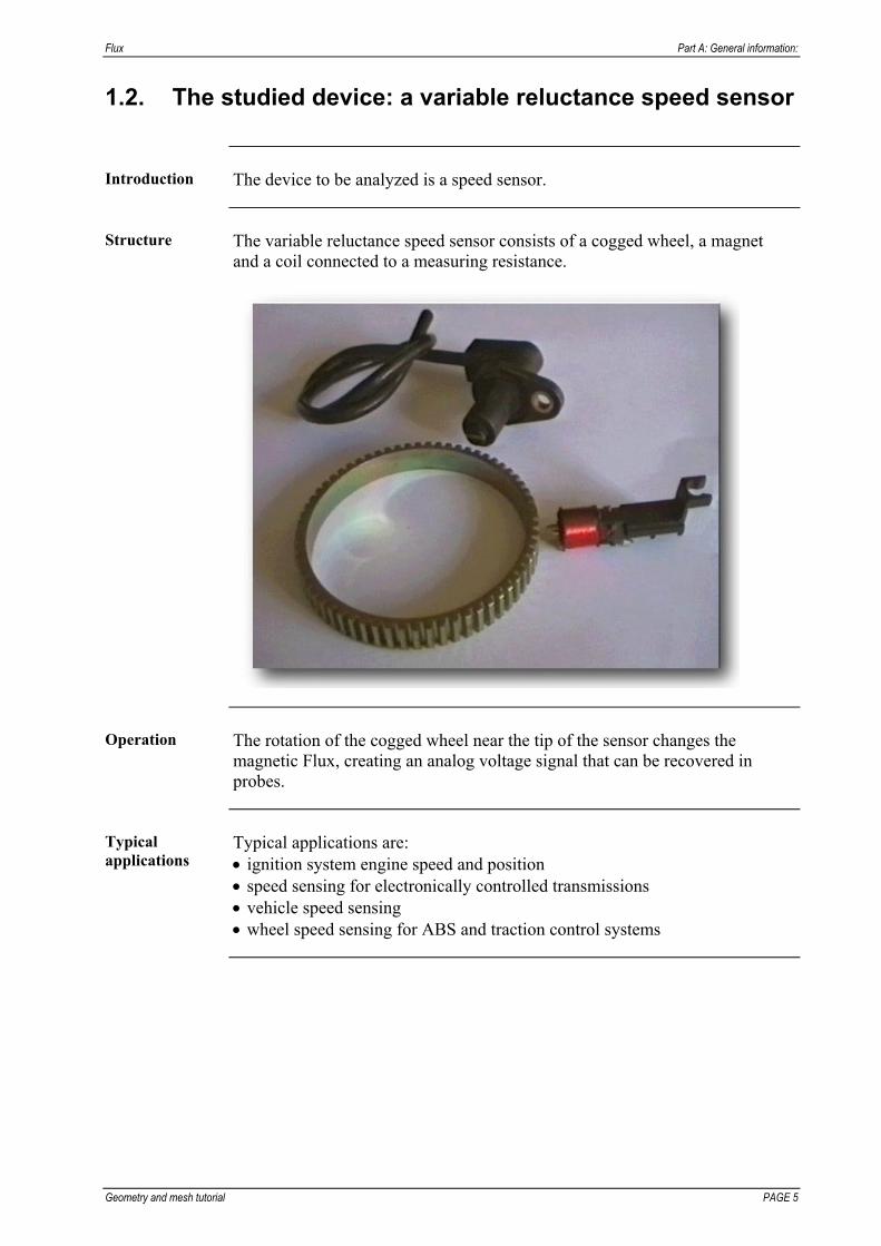
Introduction The device to be analyzed is a speed sensor.
Structure The variable reluctance speed sensor consists of a cogged wheel, a magnet
and a coil connected to a measuring resistance.
Operation The rotation of the cogged wheel near the tip of the sensor changes the
magnetic Flux, creating an analog voltage signal that can be recovered in probes.
Typical applications
Typical applications are: ignition system engine speed and position speed sensing for electronically controlled transmissions vehicle speed sensing wheel speed sensing for ABS and traction control systems

Part A: General information Flux
PAGE 6 Geometry and mesh tutorial
1.3. The device description in Flux: which strategy?
Problem How to describe the device in Flux?
Reminder: we only are interested in geometrical construction and generation of the mesh.
Geometric structure
The device consists of: one cogged wheel with three teeth two probes with a magnet and a coil around
PROBE 2
COIL 2-
COIL 2+
MAGNET 1
COIL 1-
COIL 1+
WHEEL
MAGNET 2
PROBE 1
Strategy Two strategies of description exist:
one-phase description: - description of the whole device in only one Flux project
two-phase description: - independent description of separated parts of the device in several Flux
projects - import of the independent projects (PROBE_2D.FLU and
WHEEL_BASE_2D.FLU) into one main project SENSOR_2D.FLU
The second strategy is selected in this tutorial.
Of course, the geometry can be built in ways other than the presented one. The sensor geometry is defined in this particular way in order to introduce you to the most used Flux2D features.
Continued on next page
Flux Part A: General information:
Geometry and mesh tutorial PAGE 7
1.4. Main stages for geometry description
Process (general aspects)
An outline of the general construction process is given in the two following blocks: the first process (1) is presented for ease of understanding the second process (2) is the real building process used in this document.
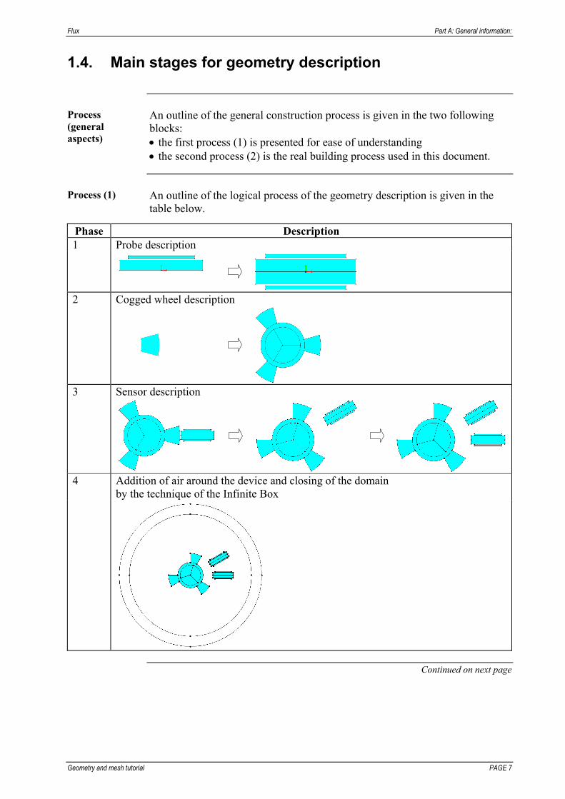
Process (1) An outline of the logical process of the geometry description is given in the
table below.
Phase Description 1 Probe description
2 Cogged wheel description
3 Sensor description
4 Addition of air around the device and closing of the domain
by the technique of the Infinite Box
Continued on next page

Part A: General information Flux
PAGE 8 Geometry and mesh tutorial
Process (2) An outline of the real process of the geometry description, used in this tutorial,
is given in the table below.
1 Probe description Project: PROBE_2D.FLU
2 Wheel base object description (elementary pattern) Project: WHEEL_BASE_2D.FLU
3 Sensor description Project: SENSOR_2D.FLU
Importation of the elementary pattern (WHEEL_BASE_2D)
Building of the whole wheel
Importation of a probe object (PROBE_2D)
Rotation of the probe and rotation of the cogged wheel
Importation of a probe object (PROBE_2D)
Addition of an Infinite Box

Flux Part A: General information:
Geometry and mesh tutorial PAGE 9
2. Get started with Flux
Introduction This chapter shows how to start working with Flux and includes a
presentation of the Flux Supervisor.
It also shows how to start the preprocessor for Flux2D.
More detailed information about Flux2D menus and commands is presented in Part B § 1.1.2 About the Flux2D window.
Contents This chapter contains the following topics:
Topic See Page Start the Flux Supervisor 11 About the Flux Supervisor 12 Open Flux2D 13

Part A: General information Flux
PAGE 10 Geometry and mesh tutorial
Flux Part A: General information:
Geometry and mesh tutorial PAGE 11
2.1. Start the Flux Supervisor
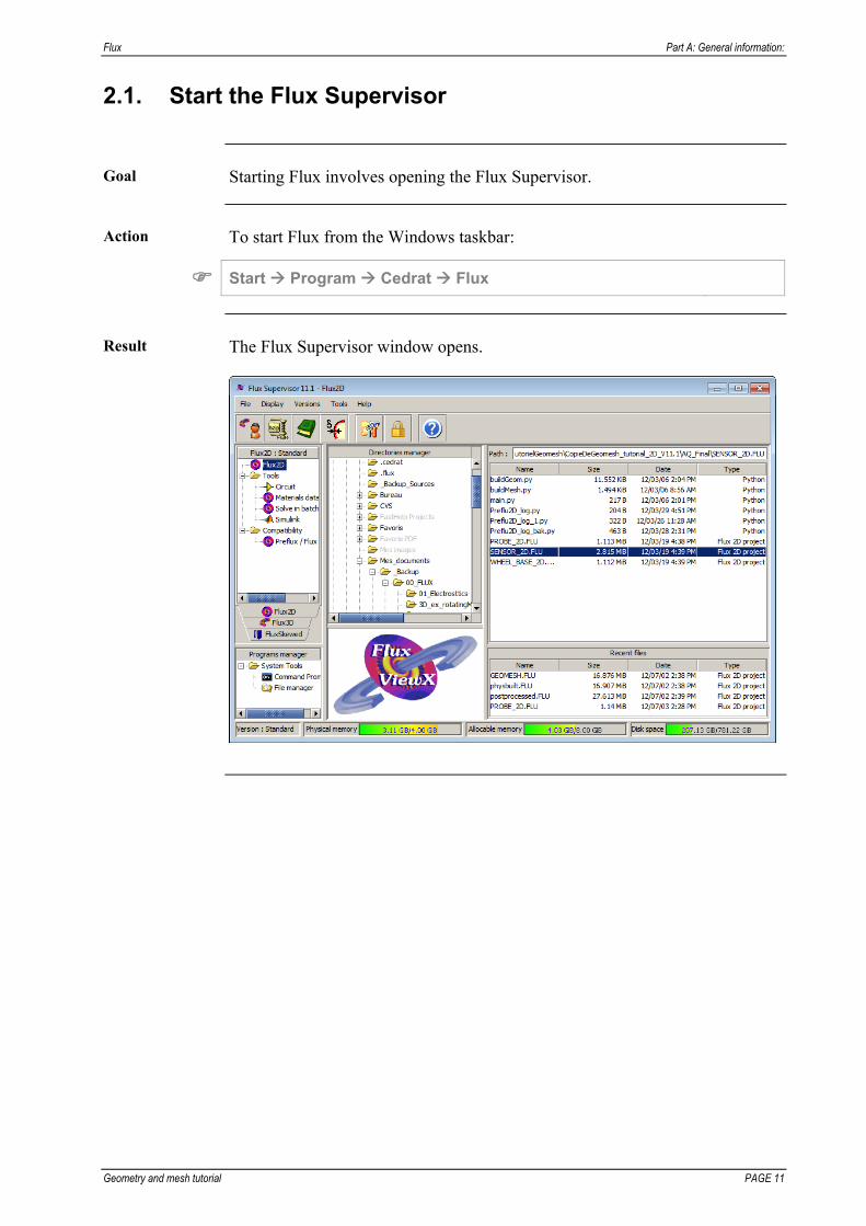
Goal Starting Flux involves opening the Flux Supervisor.
Action To start Flux from the Windows taskbar:
Start Program Cedrat Flux
Result The Flux Supervisor window opens.

Part A: General information Flux
PAGE 12 Geometry and mesh tutorial
2.2. About the Flux Supervisor
The Flux Supervisor window
The Flux Supervisor organizes all the modules for both Flux2D and Flux3D.
The Flux Supervisor window is divided into several areas. These areas are identified in the following figure and described in the table below.
Menu bar
Tool bar
Program manager
Modules
Project files
Geometry view
Directory manager
Most recent used files
Area Function Modules to list and launch all the Flux modules (Flux2D,
Circuit, etc.) Directory manager to show the computer’s complete directory Project files to display all Flux projects in the selected directory Program manager contains shortcuts to the Dos Shell and the Explorer Geometry view to display a preview of the geometry, if a project is
selected Recent files To display most recent used
Some checks before you begin
From the Flux Supervisor you should: Select the Flux 2D tab in order to access the specific Flux 2D programs. Access your working directory by selecting it in the supervisor’s directory
manager window. Verify that the title of the Program manager area is the standard version
(Flux2D: Standard). If not, in the menu bar, select Versions and check Standard.

Flux Part A: General information:
Geometry and mesh tutorial PAGE 13
2.3. Open Flux2D
Goal The preprocessor Flux2D will be opened to manage the geometry building of
the device and mesh generation.
Action To open Flux2D from the Flux Supervisor:
1. Click on the Flux2D tab
2. Select the directory of the project
3. Double-click on Geometry&Physics
Continued on next page

Part A: General information Flux
PAGE 14 Geometry and mesh tutorial
Result The PreFlux window for Flux 2D applications is opened.
There are two menus in the PreFlux window: Project and Help*.
* A new project must be created to see the complete set of PreFlux commands.

Flux Part B: Geometry and mesh description of the studied device:
Geometry and mesh tutorial PAGE 15
Part B: Geometry and mesh description of the studied device
Introduction This part B contains the description of the studied device and provide when
needed some information about the Flux software.
Contents This part contains the following topics:
Topic See Page Geometric description of the probe object 17 Geometric description of the wheel base object 75 Geometric description of the sensor 103 Mesh generation of the sensor 135 Annex 169

Part B: Geometry and mesh description of the studied device Flux
PAGE 16 Geometry and mesh tutorial
Flux Part B: Geometry and mesh description of the studied device:
Geometry and mesh tutorial PAGE 17
1. Geometric description of the probe object
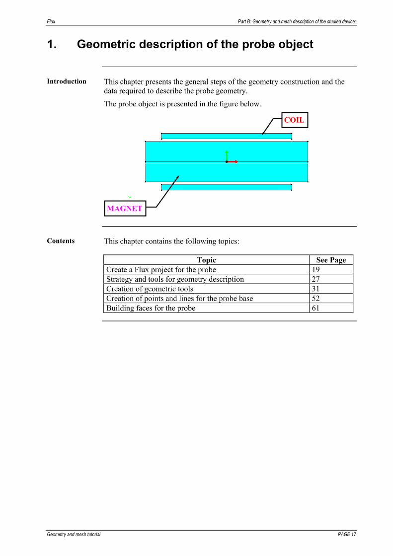
Introduction This chapter presents the general steps of the geometry construction and the
data required to describe the probe geometry.
The probe object is presented in the figure below.
COIL
MAGNET
Contents This chapter contains the following topics:
Topic See Page Create a Flux project for the probe 19 Strategy and tools for geometry description 27 Creation of geometric tools 31 Creation of points and lines for the probe base 52 Building faces for the probe 61

Part B: Geometry and mesh description of the studied device Flux
PAGE 18 Geometry and mesh tutorial

Flux Part B: Geometry and mesh description of the studied device:
Geometry and mesh tutorial PAGE 19
1.1. Create a Flux project for the probe
Introduction Each time that a Flux program is started, it is possible to open an existing
project or create a new project.
Contents This section contains the following topics:
Topic See Page Create a new project for the probe 20 About the Flux2D window 21 About the Help menu / User guide 22 About the geometry context 24 Name the project 25
Part B: Geometry and mesh description of the studied device Flux
PAGE 20 Geometry and mesh tutorial
1.1.1. Create a new project for the probe
Goal At the beginning of the geometry description a new project will be created.
Action To create a new project from the …
Project menu: 1. Click on New
OR
Project toolbar: 1. Click on the icon
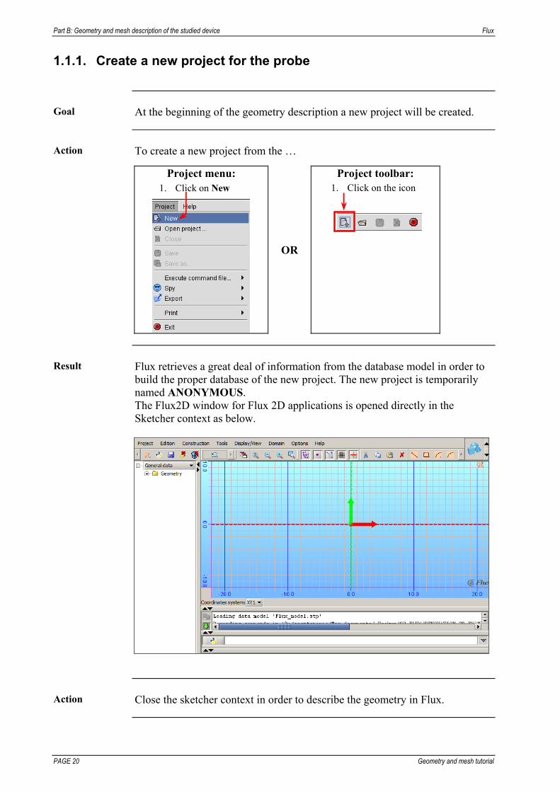
Result Flux retrieves a great deal of information from the database model in order to
build the proper database of the new project. The new project is temporarily named ANONYMOUS. The Flux2D window for Flux 2D applications is opened directly in the Sketcher context as below.
Action Close the sketcher context in order to describe the geometry in Flux.

Flux Part B: Geometry and mesh description of the studied device:
Geometry and mesh tutorial PAGE 21
1.1.2. About the Flux2D window
Flux2D window The Flux2D project window opens in the Geometry context. The Flux2D
project window has the complete set of the tools to build the geometry of the device, to mesh the computation domain and to visualize the device during different steps of the construction.
Areas The Flux2D project window is divided into three main areas. The different
areas can be resized or hid by using the arrows.
Graphic scene Data tree
History zone
Area Function Data tree displays all the problem data in a tree structure that is
expanded using the key Graphic scene displays the graphic entities History zone prints Python command instructions
Menus and toolbars
All Flux2D commands are in the menus. Toolbars include icons that are shortcuts to the most useful commands.
Menus
Toolbars

Part B: Geometry and mesh description of the studied device Flux
PAGE 22 Geometry and mesh tutorial
1.1.3. About the Help menu / User guide
Introduction There are several ways to access the user guide information:
the complete user guide the on-line help on an option
Method 1 To open the complete user’s guide in the Flux Supervisor from the …
Help menu:
1. Click on Manual…
OR
Help toolbar: 1. Click on the icon
Method 2 To open the complete user’s guide in Flux2D from the Help menu:
1. Click on Contents
Method 3 To open the on-line help about an entity from its dialog box:
1. Click on the button
Continued on next page
Flux Part B: Geometry and mesh description of the studied device:
Geometry and mesh tutorial PAGE 23
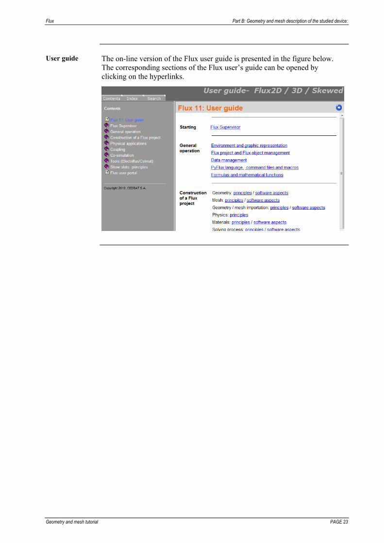
User guide The on-line version of the Flux user guide is presented in the figure below.
The corresponding sections of the Flux user’s guide can be opened by clicking on the hyperlinks.

Part B: Geometry and mesh description of the studied device Flux
PAGE 24 Geometry and mesh tutorial
1.1.4. About the geometry context
Presentation There are three contexts in Flux2D:
Context Function Geometry to build the geometry of the device Mesh to mesh the computation domain Physics* to define the materials, sources and to prepare the
regions
* The icon corresponding to the Physics context appears after the definition of the physical application
Tools of the geometry context
After having activated the geometry context, toolbars dedicated to the geometry description appear in the Flux2D window.
The different toolbars and their principal roles are briefly described below.
1 2 3 4 5
6
Geometry context toolbars Function 1 to create geometric entities 2 to propagate / extrude points, lines, etc. 3 to build faces 4 to compute geometric values 5 to check the geometry 6 to display point and line reference numbers

Flux Part B: Geometry and mesh description of the studied device:
Geometry and mesh tutorial PAGE 25
1.1.5. Name the project
Goal The new project, temporarily named ANONYMOUS, will be renamed and
saved.
Action To rename the project from the …
Project menu: 1. Click on Save or
Save as…
OR
Project toolbar: 1. Click on the icon
2. Type PROBE_2D as project name
3. Click on Save
Note: The user can choose another name for the project and change the current project directory (working directory), displayed in the Save In field at the top. A periodic data backup is recommended.

Part B: Geometry and mesh description of the studied device Flux
PAGE 26 Geometry and mesh tutorial

Flux Part B: Geometry and mesh description of the studied device:
Geometry and mesh tutorial PAGE 27
1.2. Strategy and tools for geometry description of the probe
Introduction This section shows:
the available tools for geometry building the analysis carried out for construction of the probe geometry and the
selected strategy
Contents This section contains the following topics:
Topic See Page
Available geometric tools and analysis before geometry description
28
Main stages for the probe geometry description 30
Reading advice This section presents an outline of the geometry building process of the
probe. Details on the different contents - definition of new concepts, explanation on the use of different tools, etc.- are given in the following sections.
Part B: Geometry and mesh description of the studied device Flux
PAGE 28 Geometry and mesh tutorial
1.2.1. Available geometric tools and analysis before geometry description
Available tools The tools available for the geometric construction are: geometric parameters,
coordinate systems and transformations.
Geometric tool Function geometric parameter to allow the dimensional parameter setting of parts coordinate system to facilitate the relative positioning of parts transformation to allow the construction by propagation or extrusion
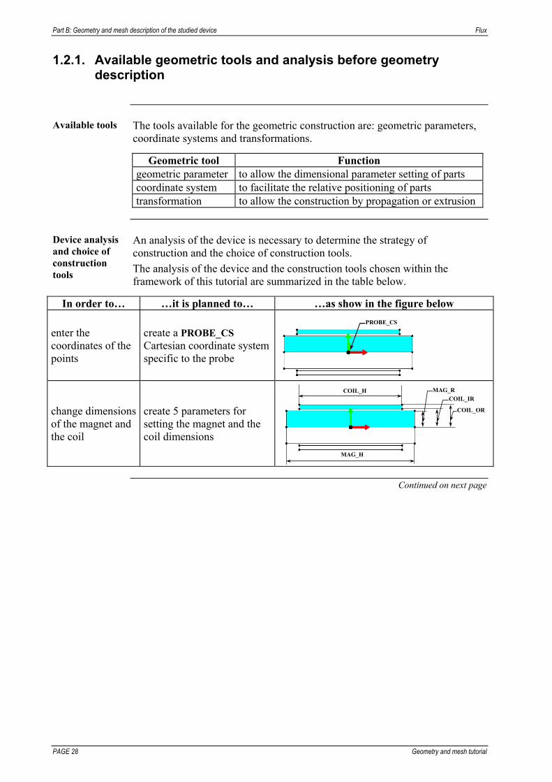
Device analysis and choice of construction tools
An analysis of the device is necessary to determine the strategy of construction and the choice of construction tools.
The analysis of the device and the construction tools chosen within the framework of this tutorial are summarized in the table below.
In order to… …it is planned to… …as show in the figure below
enter the coordinates of the points
create a PROBE_CS Cartesian coordinate system specific to the probe
PROBE_CS
change dimensions of the magnet and the coil
create 5 parameters for setting the magnet and the coil dimensions
MAG_H
COIL_H MAG_R
COIL_IR
COIL_OR
Continued on next page

Flux Part B: Geometry and mesh description of the studied device:
Geometry and mesh tutorial PAGE 29
Device analysis and choice of construction tools (continued)
In order to… …it is planned to… …as show in the figure below
locate the probe in the final project (anticipation)
create a MAIN_CS Cartesian coordinate system
(the PROBE_CS coordinate system will be attached to this coordinate system) create an ANGLE
parameter to define the angular position of the MAIN_CS coordinate system
MAIN_CS
PROBE_CS
ANGLE
simplify the geometry building
create a MIRROR transformation of the affinity type to build faces by propagation
MIRROR

Part B: Geometry and mesh description of the studied device Flux
PAGE 30 Geometry and mesh tutorial
1.2.2. Main stages for the probe geometry description
Outline An outline of the geometry building process is presented in the table below.
Stage Description
1 De-activation of Aided mesh
As the PROBE.FLU will be later imported in Sensor_2D.FLU it is necessary to de-activate the Aided mesh*
2 Creation of 6 geometric parameters
Inner radius of the coil: COIL_IR = 2.8 mm Outer radius of the coil: COIL_OR = 3.5 mm Height of the coil: COIL_H = 16 mm Radius of the magnet: MAG_R = 2.5 mm Height of the magnet: MAG_H = 20 mm Angle for the probe angular position
in the final device: ANGLE = 0°
3 Creation of 2 coordinate systems
Cartesian coordinate system: MAIN_CS (Global coordinate system for the probe positioning in the final device)
Cartesian coordinate system: PROBE_CS (Local coordinate system for the probe description)
4 Creation of points and lines for the probe base
5 Building faces for the probe base
6 Creation of 1 transformation
Affine transformation for the probe: MIRROR
7 Building faces by propagation (and preparation of the mesh generator*)
* Explanation concerning this subject is presented in “ About mesh tools” on Linked Mesh Generator)

Flux Part B: Geometry and mesh description of the studied device:
Geometry and mesh tutorial PAGE 31
1.3. Creation of geometric tools
Introduction The geometry building begins by the creation of geometric tools to build the
probe geometry: geometric parameters and coordinate systems.
The parameters and coordinate systems required to describe the geometry of the probe are presented in the figure below.
MAG_H
COIL_H MAG_R
COIL_IR
COIL_OR
MAIN_CS
PROBE_CS ANGLE
Contents This section contains the following topics:
Topic See Page Deactivate aided mesh 32 About creation an entity 33 About geometric parameters 35 Create the geometric parameters 36 About the undo command 38 About selection of graphic entities 39 About modification and deletion of an entity 41 About graphic view 44 Change the background color 46 About coordinate systems 47 Create the coordinate systems 49

Part B: Geometry and mesh description of the studied device Flux
PAGE 32 Geometry and mesh tutorial
1.3.1. Deactivate Aided mesh
Definition Aided mesh is a tool box that permits the user to quickly realize a good
quality mesh. The aided mesh (global adjustment) is activated by default on all flux projects (See About Aided mesh).
Aided mesh and imported Flux project
Aided mesh assigns specific global tool on all entities of a new project. In order not to interfere during project import to the main project, it is needed to de-activate aided mesh on project that will be imported later.
Action To deactivate the Aided mesh, from the Menu:
1. Edit the aided mesh box
2. Select “Inactivated” in the State of aided mesh field

Flux Part B: Geometry and mesh description of the studied device:
Geometry and mesh tutorial PAGE 33
1.3.2. About creation of an entity
Definition of entity
An entity is an object in the database of a Flux project. It can be: a point, a line, a coordinate system, etc. in the Geometry context a mesh point, a mesh line, etc. in the Mesh context a line region, a volume region, etc. in the Physics context
Creating process
An outline of the creating process is presented in the table below. The different steps are detailed in the blocks describing the creation of project entities.
Step Description 1 Activating the New command 2 Definition of entity attributes
Access the “New” command
The access to the New command can be carried out: from the Geometry menu bar (1) using icons from the Geometry toolbar (2) from the data tree (3)
These three methods to access the New command are presented in the following figure (with the example of creation of a geometric parameter) and described in the table below.
1
3
2
Method Description 1 point on the entity-type and click on New 2 click on the corresponding icon 3 double-click on the entity-type or right click and click on New
Continued on next page

Part B: Geometry and mesh description of the studied device Flux
PAGE 34 Geometry and mesh tutorial
Dialog box The interaction with the database is done using dialog boxes. The user can
enter information relating to the data in this box.
Entity-type: Geometric parameter
Name Comment
Characteristics
Title bar
On-line help concerning the entity
The required fields (necessary and sufficient for the definition of the entity) are marked by an asterisk *.
Flux Part B: Geometry and mesh description of the studied device:
Geometry and mesh tutorial PAGE 35
1.3.3. About geometric parameters
Principle of use Geometric parameters are entities that can be used for the geometry building
of the device, i.e. for the definition of points, coordinate systems, geometric transformations, infinite box dimensions and other geometric entities.
Defining parameters simplifies the construction of the geometry and enables modifications to be made more easily later. Many changes can be made by modifying only the definition of the parameters instead of modifying all the individual points, lines or nodes that might be built using the parameters. Parameters also can modify the scale of the geometry through their relationship with coordinate systems.
Definition of parameters
The geometric parameters are defined by the name and the algebraic expressions.
The algebraic expressions may contain: constants arithmetic operators (+, -, *, /, **) arithmetic functions allowed in FORTRAN (SQRT, LOG, SIN, etc.)* other parameters combinations of any of these
* Caution: ATAN2D is preferred over ATAN in order to have a better accuracy.
Parameters and measurement units
Please note that parameters are independent of any unit of measurement. In other words, the numerical value entered for a parameter is not changed when the unit of measurement is changed. Any measurement unit associated with a parameter derives from the coordinate system in which the parameter is used. For example, a parameter's value may be 10 in a coordinate system with millimeters as units. This parameter's value is still 10 whether the coordinate system's units are changed to inches or meters or kilometers or any other available unit. Thus, when you use parameters, you can also modify the scale of a geometric feature without reentering each point or item.

Part B: Geometry and mesh description of the studied device Flux
PAGE 36 Geometry and mesh tutorial
1.3.4. Create the geometric parameters
Goal Six parameters, required to describe the geometry of the probe, are presented
in the figure below.
MAG_H
COIL_H MAG_R
COIL_IR
COIL_ORANGLE
MAGNET base
COIL base
Data The table below contains the values of the geometric parameters.
Geometric parameters
Name Comment Expression COIL_IR Inner radius of the coil 2.8 COIL_OR Outer radius of the coil 3.5 COIL_H Height of the coil 16 ANGLE Angle of the probe position 0 MAG_R Radius of the magnet 2.5 MAG_H Height of the magnet 20
Continued on next page

Flux Part B: Geometry and mesh description of the studied device:
Geometry and mesh tutorial PAGE 37
Action To create the geometric parameters from the …
Data tree: 1. Double-click
on Geometric parameter
OR
Geometry toolbar: 1. Click on the icon
2. Type COIL_IR as name 3. Type Inner radius of the coil as
comment 4. Type 2.8 as algebraic expression for
the parameter 5. Click on OK
6. Repeat steps 2 to 5 in the new dialog, entering data for the remaining entities. (see the table on the previous page)
…
7. Click on Cancel to quit the sequence
Result The geometric parameters are listed in the data tree:
Notice too, that as you move your cursor over the parameter names, the comments are displayed to help you to identify the parameters.
Part B: Geometry and mesh description of the studied device Flux
PAGE 38 Geometry and mesh tutorial
1.3.5. About the undo command
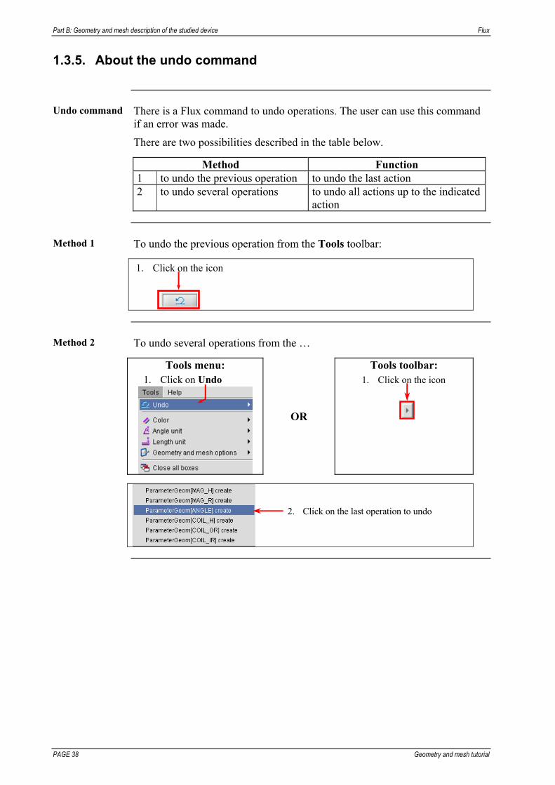
Undo command There is a Flux command to undo operations. The user can use this command
if an error was made.
There are two possibilities described in the table below.
Method Function 1 to undo the previous operation to undo the last action 2 to undo several operations to undo all actions up to the indicated
action
Method 1 To undo the previous operation from the Tools toolbar:
1. Click on the icon
Method 2 To undo several operations from the …
Tools menu:
1. Click on Undo
OR
Tools toolbar: 1. Click on the icon
2. Click on the last operation to undo
Flux Part B: Geometry and mesh description of the studied device:
Geometry and mesh tutorial PAGE 39
1.3.6. About selection of graphic entities
Overview of selection modes
Selection of entities can be done with the following selection modes: graphic selection (with the mouse)
- in the data tree for all entities - in the graphic scene for graphic entities
identifier selection (by name / by number) advanced selection (by criterion / by choice)
Graphic selection process
An outline of the selection process for graphic entities is presented in the table below. The different steps are detailed in the blocks describing the creation of project entities.
Step Description 1 Activating of the selection filter 2 Selection of the entity in the graphic scene
Selection filter A selection filter makes possible to identify the selectable entity-type.
For the graphic entities, the selection filter can be activated by the commands from the Selection menu or from the Selection toolbar.
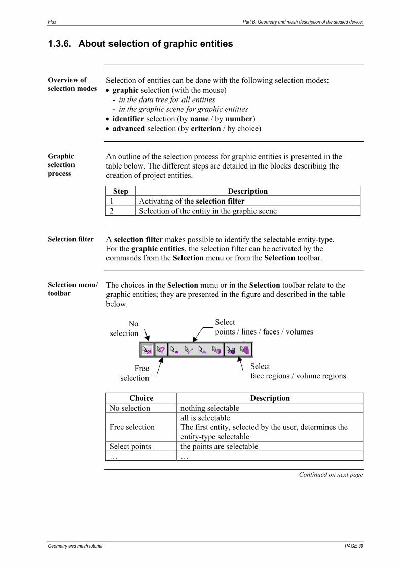
Selection menu/ toolbar
The choices in the Selection menu or in the Selection toolbar relate to the graphic entities; they are presented in the figure and described in the table below.
Noselection
Freeselection
Select points / lines / faces / volumes
Select face regions / volume regions
Choice Description No selection nothing selectable
Free selection all is selectable The first entity, selected by the user, determines the entity-type selectable
Select points the points are selectable … …
Continued on next page

Part B: Geometry and mesh description of the studied device Flux
PAGE 40 Geometry and mesh tutorial
Step 1: activating of the selection filter
The activating of the selection filter can be carried out: from the Select menu (1) using icons from the Select toolbar (2)
These two methods to activate the selection filter are presented in the following figure and described in the table below.
1
2
Step 2: selection in the graphic scene
Click on the specific graphic entity to select the entity in the graphic scene. The selected entity is highlighted.
Flux Part B: Geometry and mesh description of the studied device:
Geometry and mesh tutorial PAGE 41
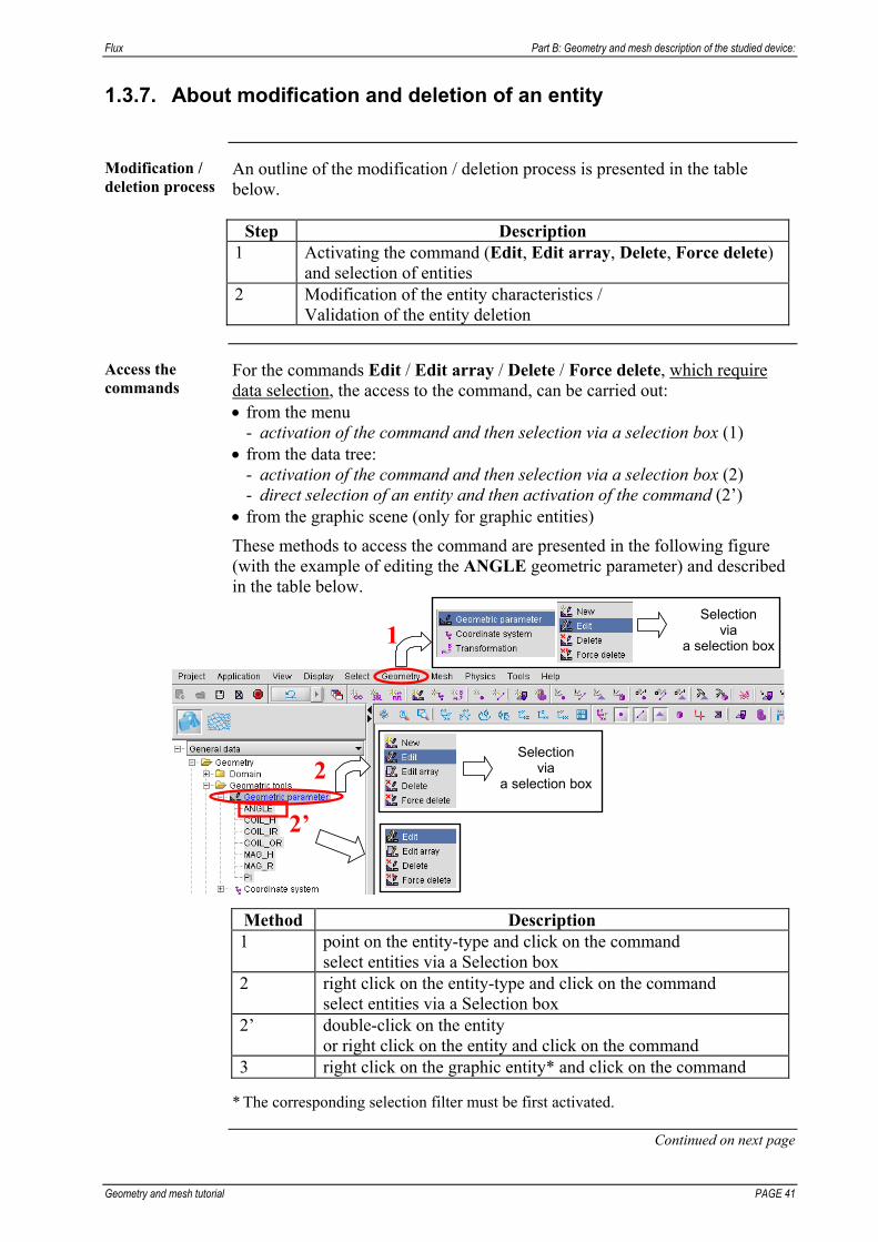
1.3.7. About modification and deletion of an entity
Modification / deletion process
An outline of the modification / deletion process is presented in the table below.
Step Description
1 Activating the command (Edit, Edit array, Delete, Force delete) and selection of entities
2 Modification of the entity characteristics / Validation of the entity deletion
Access the commands
For the commands Edit / Edit array / Delete / Force delete, which require data selection, the access to the command, can be carried out: from the menu
- activation of the command and then selection via a selection box (1) from the data tree:
- activation of the command and then selection via a selection box (2) - direct selection of an entity and then activation of the command (2’)
from the graphic scene (only for graphic entities)
These methods to access the command are presented in the following figure (with the example of editing the ANGLE geometric parameter) and described in the table below.
1
2
Selection via
a selection box
2’
Selection via
a selection box
Method Description 1 point on the entity-type and click on the command
select entities via a Selection box 2 right click on the entity-type and click on the command
select entities via a Selection box 2’ double-click on the entity
or right click on the entity and click on the command 3 right click on the graphic entity* and click on the command
* The corresponding selection filter must be first activated.
Continued on next page

Part B: Geometry and mesh description of the studied device Flux
PAGE 42 Geometry and mesh tutorial
Edition mode To check the data, the user needs to edit (and modify if necessary) the entities
created.
There are two modes of edition: the edition in a dialog box is used to check and to modify the
characteristics of one entity
Entity-type
Name Comment
Type (1)
Characteristics
Entity
Type (2)
On-line help concerning the entity
the edition in a data array is used to check and to modify the characteristics of a group of entities
Entity-type
Name Comment
Type (1)
Characteristics
Entities: [CORE], [MAIN]
Type (2)
Structure(Database)
Information relating to the
group of entities
Information relating to the entity [CORE]
Information relating to the entity [MAIN]
Continued on next page

Flux Part B: Geometry and mesh description of the studied device:
Geometry and mesh tutorial PAGE 43
Deletion mode The user sometimes needs to delete entities. He can easily delete an entity if it
is an independent entity. However, very often, the entity is connected to other entities and the deletion of the entity can cause the deletion of all the connected entities.
There are thus two modes of deletion: the simple deletion:
is carried out on independent entities (non connected with other entities) the in force deletion :
is carried out on any entity.
These two modes are described in the table below:
Mode Destroyable entity What is destroyed simple independent selected entity in force any selected entity + entities connected to it

Part B: Geometry and mesh description of the studied device Flux
PAGE 44 Geometry and mesh tutorial
1.3.8. About graphic view
Introduction When referring to the graphic representation of a device, we are interested in:
the different entities and their appearance: points and their visibility, lines and their color, faces, surface elements, etc.
the type of displayed view: side view, top view, bottom view, global view, etc. and its position and dimensions in the graphic display zone.
How to modify a view
There are three methods to modify the view in the graphic scene. The modifications can be made: from the View menu (1) using icons from the View toolbar (2) using the mouse (3)
1
3
2
Continued on next page
Flux Part B: Geometry and mesh description of the studied device:
Geometry and mesh tutorial PAGE 45
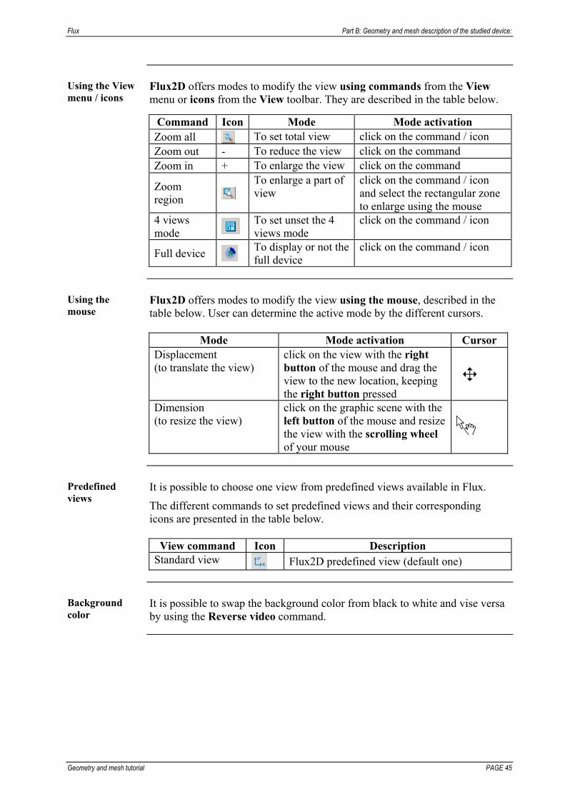
Using the View menu / icons
Flux2D offers modes to modify the view using commands from the View menu or icons from the View toolbar. They are described in the table below.
Command Icon Mode Mode activation Zoom all To set total view click on the command / icon Zoom out - To reduce the view click on the command Zoom in + To enlarge the view click on the command
Zoom region
To enlarge a part of view
click on the command / icon and select the rectangular zone to enlarge using the mouse
4 views mode
To set unset the 4 views mode
click on the command / icon
Full device To display or not the full device
click on the command / icon
Using the mouse
Flux2D offers modes to modify the view using the mouse, described in the table below. User can determine the active mode by the different cursors.
Mode Mode activation Cursor
Displacement (to translate the view)
click on the view with the right button of the mouse and drag the view to the new location, keeping the right button pressed
Dimension (to resize the view)
click on the graphic scene with the left button of the mouse and resize the view with the scrolling wheel of your mouse
Predefined views
It is possible to choose one view from predefined views available in Flux.
The different commands to set predefined views and their corresponding icons are presented in the table below.
View command Icon Description
Standard view Flux2D predefined view (default one)
Background color
It is possible to swap the background color from black to white and vise versa by using the Reverse video command.

Part B: Geometry and mesh description of the studied device Flux
PAGE 46 Geometry and mesh tutorial
1.3.9. Change the background color
Goal To better visualize the geometry, the background color will be changed.
Action To change the background color from the View menu:
1. Click on Reverse video

Flux Part B: Geometry and mesh description of the studied device:
Geometry and mesh tutorial PAGE 47
1.3.10. About coordinate systems
Introduction All geometric features are defined within a specific coordinate system.
Defining our own coordinate systems enables us to describe and modify the geometry much more easily.
Types of coordinate systems
The different types of coordinate systems for 2D domain and associated coordinates are presented below.
Cartesian coordinate system Coordinates (x, y)
Cylindrical coordinate system Coordinates (r, )
y
x
p
r
p
Reference coordinate systems
It is possible to distinguish the following coordinate systems: The global coordinate system is the coordinate system where all
computations are performed. It is inaccessible to the user. The global coordinate system is a universal Cartesian coordinate system using meters as the length unit and degrees as the angle unit.
The working coordinate systems are coordinate systems created by the user to cover the study needs. The working coordinate systems are defined: - with respect to the Global coordinate system, when they refer to the
global coordinate system - with respect to a Local coordinate system, when they refer to other
coordinate systems. All entities are defined in the working coordinate systems (user coordinate systems) and are evaluated in the global coordinate system for calculations.
Coordinate system units
The user can define the length and angle units for a coordinate system defined with respect to the global coordinate system (millimeter and degree by default).
A coordinate system defined with respect to the local coordinate system inherits the units of the reference coordinate system (parent coordinate system).
Continued on next page

Part B: Geometry and mesh description of the studied device Flux
PAGE 48 Geometry and mesh tutorial
Predefined coordinate system
To assist the user, Flux provides a default coordinate system XY1. It is created for every new project. It is possible to rename it, to modify it or to delete it.
XY1 is the coordinate system of Cartesian type and defined with respect to the global coordinate system.
Coordinate system XY1 Characteristics Y
X
y
x
Origin of coordinate system: first component: 0 second component: 0 Rotation angle: about Z axis: 0

Flux Part B: Geometry and mesh description of the studied device:
Geometry and mesh tutorial PAGE 49
1.3.11. Create the coordinate systems
Goal Two coordinate systems, required to describe the geometry of the probe, are
presented in the figure below.
MAIN_CS
PROBE_CS
32 mm
Data The tables below describe the coordinate systems.
Cartesian coordinate system type defined with respect to the Global system
Origin coord.
Rotation angle Name Comment Units
X Y About Z
MAIN_CS Main coordinate system
millimeter/ degree
0 0 ANGLE
Cartesian coordinate system type defined with respect to the Local system
Origin coord.
Rotation angle Name Comment
Parent coord. system X Y About Z
PROBE_CS Probe coordinate system
MAIN_CS 32 0 0
Continued on next page

Part B: Geometry and mesh description of the studied device Flux
PAGE 50 Geometry and mesh tutorial
Action To create the coordinate systems from the …
Data tree: 1. Double-click
on Coordinate system
OR
Geometry toolbar: 1. Click on the icon
2. Type MAIN_CS as name of coordinate system
3. Type Main coordinate system as associated comment
4. Select Cartesian as type of coordinate system
5. Select Global as definition of coordinate system
6. Select MILLIMETER as length unit
7. Select DEGREE as angle unit 8. Type 0 as first coordinate 9. Type 0 as second coordinate
10. Type ANGLE as rotation angle
about Z axis 11. Click on OK
Continued on next page

Flux Part B: Geometry and mesh description of the studied device:
Geometry and mesh tutorial PAGE 51
12. Type PROBE_CS as name of coordinate system
13. Type Probe coordinate system as comment
14. Select Cartesian as type 15. Select Local as definition of
coordinate system 16. Select MAIN_CS as parent
coordinate system
17. Type 32 as first coordinate 18. Type 0 as second coordinate 19. Type 0 as rotation angle about Z
axis 20. Click on OK
21. Click on Cancel to quit the sequence
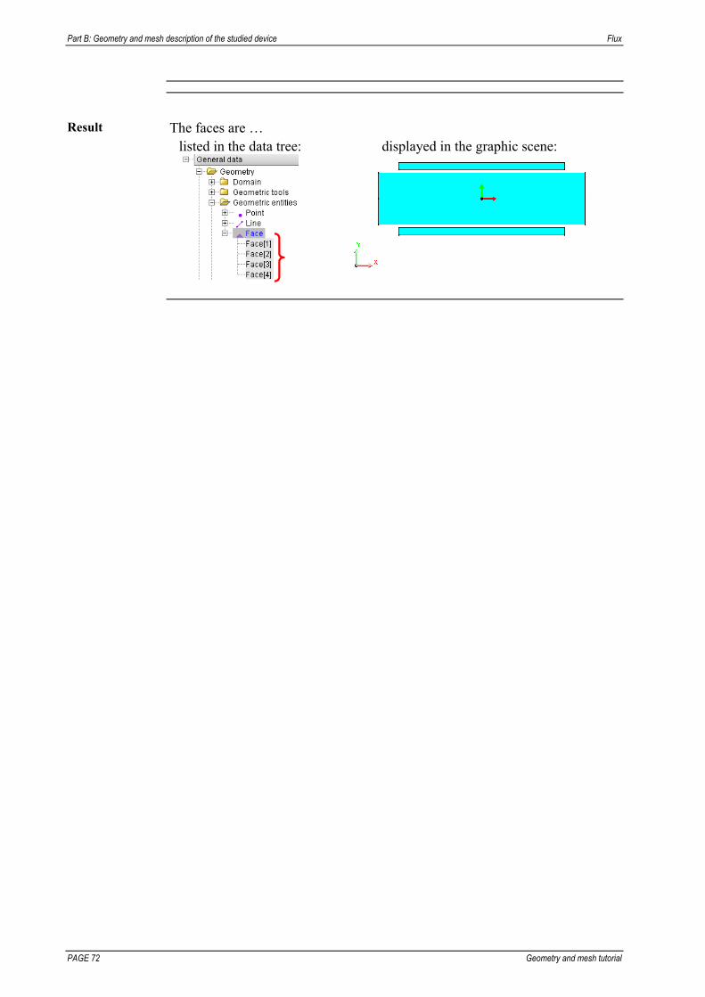
Result The two new coordinate systems are … listed in the data tree: displayed in the graphic scene*:
PROBE_CSMAIN_CS
* use the Zoom all command or (see § About graphic view).
Part B: Geometry and mesh description of the studied device Flux
PAGE 52 Geometry and mesh tutorial
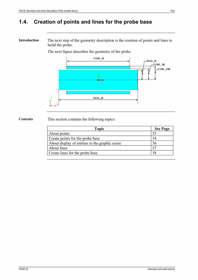
1.4. Creation of points and lines for the probe base
Introduction The next step of the geometry description is the creation of points and lines to
build the probe.
The next figure describes the geometry of the probe.
MAG_H
COIL_HMAG_R
COIL_IR
COIL_OR
Contents This section contains the following topics:
Topic See Page About points 53 Create points for the probe base 54 About display of entities in the graphic scene 56 About lines 57 Create lines for the probe base 58

Flux Part B: Geometry and mesh description of the studied device:
Geometry and mesh tutorial PAGE 53
1.4.1. About points
Points A point can be created:
as a set of coordinates in a specified coordinate system as an image of an existing point through a geometric transformation within the propagation or extrusion from other entities
Point coordinates
A point could be defined by its coordinates in a coordinate system (see § About coordinate systems).
Point defined by propagation
A point could be defined by propagation from another point using a transformation.
translation
origin point
created point
Point number The number to identify the point is automatically allocated by Flux during the
point creation.
Part B: Geometry and mesh description of the studied device Flux
PAGE 54 Geometry and mesh tutorial
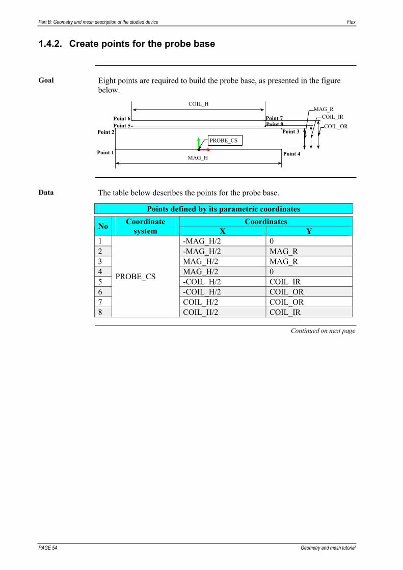
1.4.2. Create points for the probe base
Goal Eight points are required to build the probe base, as presented in the figure
below.
Point 1 MAG_H
COIL_H
Point 2 Point 3
Point 4
PROBE_CS
Point 5 Point 6 Point 7
Point 8
MAG_R COIL_IR
COIL_OR
Data The table below describes the points for the probe base.
Points defined by its parametric coordinates
Coordinates No
Coordinate system X Y
1 -MAG_H/2 0 2 -MAG_H/2 MAG_R 3 MAG_H/2 MAG_R 4 MAG_H/2 0 5 -COIL_H/2 COIL_IR 6 -COIL_H/2 COIL_OR 7 COIL_H/2 COIL_OR 8
PROBE_CS
COIL_H/2 COIL_IR
Continued on next page

Flux Part B: Geometry and mesh description of the studied device:
Geometry and mesh tutorial PAGE 55
Action To create the points from the …
Data tree: 1. Double-click on Point
OR
Geometry toolbar:
1. Click on the icon
2. In the Geometric Definition tab
select Point defined by its parametric coordinates as type of point
3. Select PROBE_CS as coordinate system
4. Type -MAG_H/2 as first coordinate
5. Type 0 as second coordinate
6. Click on OK
7. Repeat steps 4 to 7 in the new dialog, entering data for the remaining entities (see the table on the previous page)
…
8. Click on Cancel to quit the sequence
Result The points are … listed in the data tree:
displayed in the graphic scene:
Part B: Geometry and mesh description of the studied device Flux
PAGE 56 Geometry and mesh tutorial
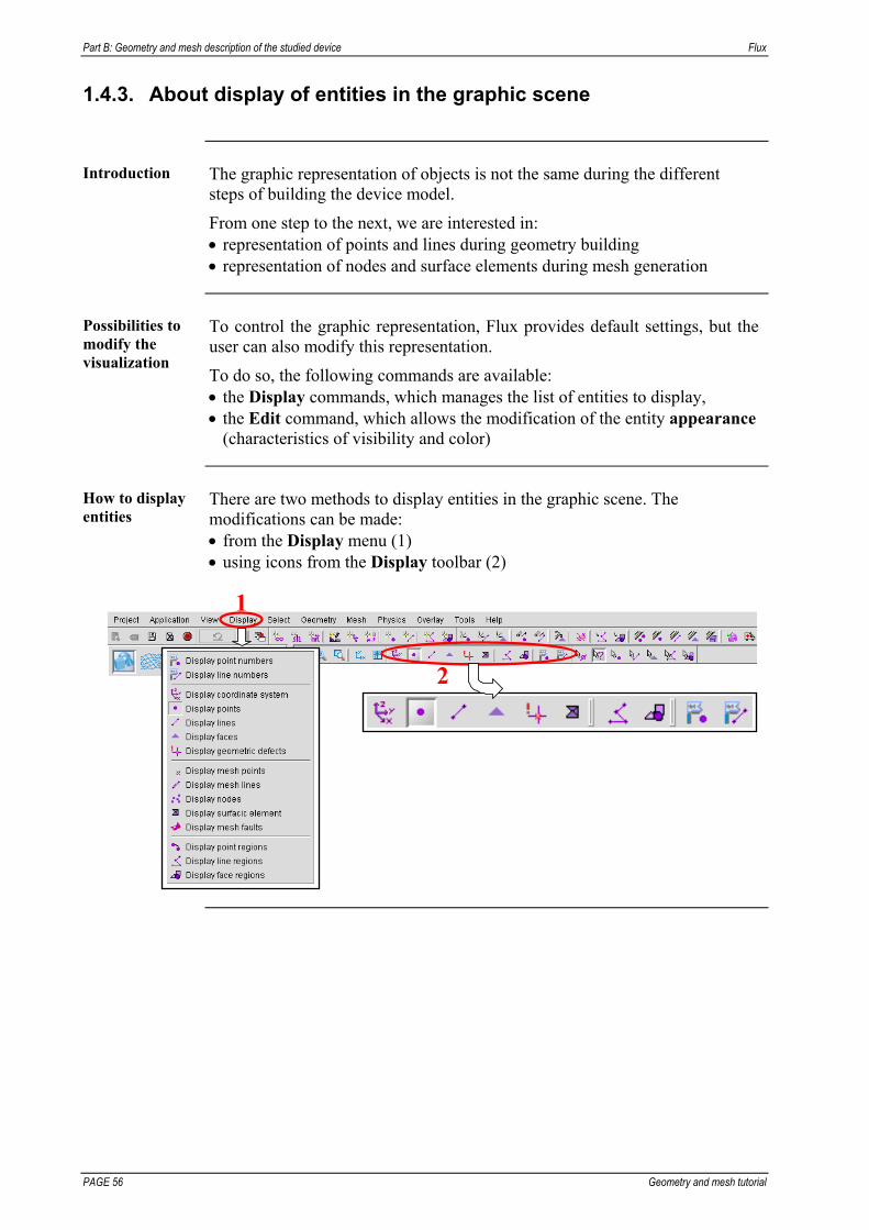
1.4.3. About display of entities in the graphic scene
Introduction The graphic representation of objects is not the same during the different
steps of building the device model.
From one step to the next, we are interested in: representation of points and lines during geometry building representation of nodes and surface elements during mesh generation
Possibilities to modify the visualization
To control the graphic representation, Flux provides default settings, but the user can also modify this representation.
To do so, the following commands are available: the Display commands, which manages the list of entities to display, the Edit command, which allows the modification of the entity appearance
(characteristics of visibility and color)
How to display entities
There are two methods to display entities in the graphic scene. The modifications can be made: from the Display menu (1) using icons from the Display toolbar (2)
1
2

Flux Part B: Geometry and mesh description of the studied device:
Geometry and mesh tutorial PAGE 57
1.4.4. About lines
Lines Lines can be created: manually (choice of line type – segment or arc - and entering extremity
points) by propagation from existing lines using a transformation by extrusion from existing points using a transformation within the propagation or extrusion from other entities
Segments Segments are defined by starting and ending points. It does not matter if you
swap the starting and ending points.
Circle arcs Circle arcs can be defined in different ways:
either in a coordinate system: The arc is included in a plane parallel to the XOY plane. It is counter-clockwise oriented around an axis parallel to the OZ axis.
starting point
ending point
center point
radius
angle
or by three points: The arc is drawn around a triangle defined by three points. It is oriented in the direction imposed by three points.
ending point
starting point
middle point
Number The number to identify the line is automatically allocated by Flux during the line creation.

Part B: Geometry and mesh description of the studied device Flux
PAGE 58 Geometry and mesh tutorial
1.4.5. Create lines for the probe base
Goal Eight straight segments are required to connect each point and create closed
outlines of the magnet and coil bases.
The order to create the lines is presented in the figure below.
Line 1 Line 3
Line 4
Line 6 Line 7 Line 8
MAGNET base
COIL base
Line 2
Line 5
Data The table below describes the lines for the probe base.
Segment defined by starting and ending points
No Starting point Ending point 1 1 2 2 2 3 3 3 4 4 4 1 5 5 6 6 6 7 7 7 8 8 8 5
Continued on next page

Flux Part B: Geometry and mesh description of the studied device:
Geometry and mesh tutorial PAGE 59
Action To create the lines from the …
Data tree: 1. Double-click on Line
OR
Geometry toolbar:
1. Click on the icon
2. In the Geometric Definition tab
select Segment defined by starting and ending points as type of the line
3. Click on Point 1 in the graphic scene
=> its reference number enters as starting point
4. Click on Point 2 in the graphic scene=> its reference number enters as ending point
5. Repeat steps 3 to 4 in the new reduced dialog, entering data for the remaining entities (see the table on the previous page)
…
6. Click on Cancel to quit the sequence
Result The lines are … listed in the data tree:
displayed in the graphic scene:

Part B: Geometry and mesh description of the studied device Flux
PAGE 60 Geometry and mesh tutorial
Flux Part B: Geometry and mesh description of the studied device:
Geometry and mesh tutorial PAGE 61
1.5. Building faces for the probe
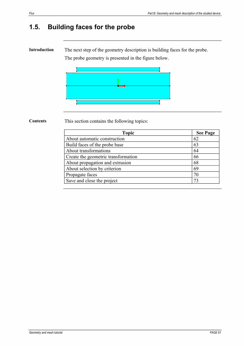
Introduction The next step of the geometry description is building faces for the probe.
The probe geometry is presented in the figure below.
Contents This section contains the following topics:
Topic See Page About automatic construction 62 Build faces of the probe base 63 About transformations 64 Create the geometric transformation 66 About propagation and extrusion 68 About selection by criterion 69 Propagate faces 70 Save and close the project 73

Part B: Geometry and mesh description of the studied device Flux
PAGE 62 Geometry and mesh tutorial
1.5.1. About automatic construction
Introduction The faces are automatically created and identified using the algorithms of
automatic construction.
Principle: overview
The principle of automatic face construction: First, Flux computes all the existing surfaces and determines which surfaces
the points and the lines belong to. (In Flux; a surface is defined by two lines connected to a shared point.)*
Next, the automatic face construction is carried out by a method of identification of closed contours. (In Flux, a face is defined by his contour and from one surface.)
About faces The faces created by Flux using the automatic construction algorithms are
faces contained by planar, cylindrical or conical surfaces. These faces are named automatic faces.
* In Flux2D, there is only one surface which is the 2D plane.

Flux Part B: Geometry and mesh description of the studied device:
Geometry and mesh tutorial PAGE 63
1.5.2. Build faces of the probe base
Goal The faces will be automatically built by Flux2D.
Action To build faces from the …
Geometry menu: 1. Point on Build and click on Build faces
OR
Geometry toolbar: 1. Click on the icon
Result The faces are … listed in the data tree:
displayed in the graphic scene:
Part B: Geometry and mesh description of the studied device Flux
PAGE 64 Geometry and mesh tutorial
1.5.3. About transformations
Principle of use Transformations are geometric functions that allow the creation of new
objects from existing objects.
Various functions
The various available functions are: translation rotation affinity helix composed
Note: Only the transformation functions used in this tutorial are described here. Refer to the User’s guide for more information about transformations.
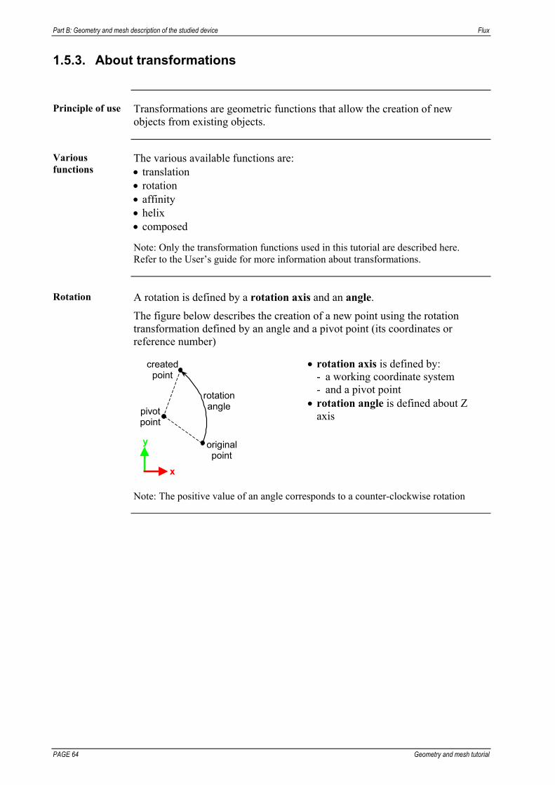
Rotation A rotation is defined by a rotation axis and an angle.
The figure below describes the creation of a new point using the rotation transformation defined by an angle and a pivot point (its coordinates or reference number)
rotation angle
original point
y
x
created point
pivot point
rotation axis is defined by: - a working coordinate system - and a pivot point
rotation angle is defined about Z axis
Note: The positive value of an angle corresponds to a counter-clockwise rotation

Flux Part B: Geometry and mesh description of the studied device:
Geometry and mesh tutorial PAGE 65
Affinity Affinity is defined with respect to a point or to a straight line.
The result of this transformation application depends on the affinity ratio, as presented in the table below.
Ratio Result k = -1 symmetry k = 1 identity k = 0 projection k >1 increasing (increasing affinity) 0< k < 1 reducing (reducing affinity) k < -1 increasing (increasing negative affinity) -1< k < 0 reducing (reducing negative affinity)
The examples below describe the creation of new lines using two different affinity transformations: Affine transformation with respect to a point
y
original line
center point of the affinity
(0.5)
x
(1)
(-1)
(-0.5)
(0)
Caution: Applying an affinity transformation with respect to a point with the scaling factor equal 0 causes an error, because the line is degenerated and reduced to a point.
Affine transformation with respect to a line defined by two points
(-1)
(-0.5)
(0)
original line
(1)
affinity line
y
x

Part B: Geometry and mesh description of the studied device Flux
PAGE 66 Geometry and mesh tutorial
1.5.4. Create the geometric transformation
Goal An affine transformation with respect to a line defined by 2 points is
required to build the probe geometry.
The points, defined the symmetry line of the transformation, are shown in the following figure:
Point 4 Point 1
Symmetry line
Data The characteristics of the transformation are shown in the following table:
Affine transformation with respect to a line defined by 2 points
Name Comment 1st point 2nd point Scaling factor
MIRROR Symmetry transformation for the probe
1 4 -1
Continued on next page

Flux Part B: Geometry and mesh description of the studied device:
Geometry and mesh tutorial PAGE 67
Action To create the transformation from the …
Data tree: 1. Double-click
on Transformation
OR
Geometry toolbar: 1. Click on the icon
2. Type MIRROR as name 3. Type Symmetry transformation
for the probe as comment 4. Select Affine transformation with
respect to a line defined by 2 points as type
5. Type 1 as first point of straight line6. Type 4 as second point of straight
line 7. Type -1 as scaling factor 8. Click on OK
9. Click on Cancel to quit the sequence
Result The transformation is listed in the data tree:
Part B: Geometry and mesh description of the studied device Flux
PAGE 68 Geometry and mesh tutorial
1.5.5. About propagation and extrusion
Definition The construction by propagation / extrusion is a building method that constructs new geometric entities, based on existing entities, by using a geometric transformation like translation, rotation, etc.
We deal with: propagation, when the image object, generated by transformation, is not
connected by lines to the source object extrusion, when the image object, generated by transformation, is
connected by lines to the source object
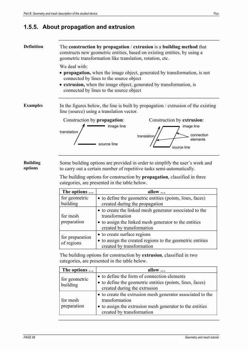
Examples In the figures below, the line is built by propagation / extrusion of the existing
line (source) using a translation vector.
Construction by propagation:
translation
source line
image line
Construction by extrusion:
translation
source line
connection elements
image line
Building options
Some building options are provided in order to simplify the user’s work and to carry out a certain number of repetitive tasks semi-automatically.
The building options for construction by propagation, classified in three categories, are presented in the table below.
The options … allow … for geometric building
to define the geometric entities (points, lines, faces) created during the propagation
for mesh preparation
to create the linked mesh generator associated to the transformation
to assign the linked mesh generator to the entities created by transformation
for preparation of regions
to create surface regions to assign the created regions to the geometric entities
created by transformation
The building options for construction by extrusion, classified in two categories, are presented in the table below.
The options … allow …
for geometric building
to define the form of connection elements to define the geometric entities (points, lines, faces)
created during the extrusion
for mesh preparation
to create the extrusion mesh generator associated to the transformation
to assign the extrusion mesh generator to the entities created by transformation

Flux Part B: Geometry and mesh description of the studied device:
Geometry and mesh tutorial PAGE 69
1.5.6. About selection by criterion
Definition / use One speaks about selection by criterion when the selection is carried out by
the intermediary of the existing relations between the various entities (points belonging to a line, ...) or characteristics, common to several entities (faces with the same color, faces on the same surface, ...).
Operation mode
The selection by criterion is available on the level of selection boxes and is carried out in two stages as presented in the table below.
Stage Description 1 From a selection box:
opening the criteria list (with the button ) and selection of a criterion
2 From a specific (with logical operators) selection box: selection of entities (graphic selection, by identifier or criterion) with applying selection operators to the group of entities
Selection criteria
The selection criteria are presented in the tables below.
General criteria The option … allows …
Select all selection of all entities Clean selection unselection of all the entities previously selected Select last instance selection of the last selected entity Selection by coordinates
selection of the nearest entity to the entered coordinates
Specific criteria (implying the use of the operators) The selection by … allows the selection of all the entities …
line / face / volume belonging to a line / face / volume surface belonging to a surface (defined by a face) linear / face / volume region belonging to a linear / face / volume region mechanical set belonging to a mechanical set color defined by a color visibility defined by a visibility (visible or invisible) nature defined by a nature (standard, in air, no exist) discretization defined by a discretization (point or line)
Selection operators
To manage the logical operations on the groups of the selected entities, the user disposes the selection operators introduced in the table below.
Operator Function Exclude to remove entities from the list Union to add entities in the list Intersect to carry out the intersection of two groups of selection

Part B: Geometry and mesh description of the studied device Flux
PAGE 70 Geometry and mesh tutorial
1.5.7. Propagate faces
Goal The MIRROR transformation will be applied once to propagate two faces, as
shown in the following figure.
Face 1
Face 2
Continued on next page

Flux Part B: Geometry and mesh description of the studied device:
Geometry and mesh tutorial PAGE 71
Action To propagate the face from the …
Geometry menu: 1. Point on Propagate
and click on Propagate faces
OR
Geometry toolbar: 1. Click on the icon
2. Click on 3. Click on Select all
=> face reference numbers enter 4. Select MIRROR as transformation5. Type 1 as number of times to apply
the transformation 6. Select Add Faces, Lines and
Points as building options for propagation
7. Click on OK
8. Click on Cancel to quit the sequence
Continued on next page
Part B: Geometry and mesh description of the studied device Flux
PAGE 72 Geometry and mesh tutorial
Result The faces are … listed in the data tree:
displayed in the graphic scene:

Flux Part B: Geometry and mesh description of the studied device:
Geometry and mesh tutorial PAGE 73
1.5.8. Save and close the project
Goal The current project will be saved and closed.
Action To save and close the PROBE_2D.FLU project from the …
Project menu: 1. Click on Close
OR
Project toolbar: 1. Click on the icon
2. Click on Yes

Part B: Geometry and mesh description of the studied device Flux
PAGE 74 Geometry and mesh tutorial

Flux Part B: Geometry and mesh description of the studied device:
Geometry and mesh tutorial PAGE 75
2. Geometric description of the wheel base object
Introduction This chapter presents the general steps of the geometry construction and the
data required to describe the wheel base geometry.
The wheel base object is presented in the figure below.
TOOTH
Contents This chapter contains the following topics:
Topic See Page Create a Flux project for the wheel base 77 Strategy and tools for geometry description of the wheel base object
79
Creation of geometric tools 83 Creation of points and lines for the wheel base 89 Building the face for the wheel base 95 Creation of the transformation 97

Part B: Geometry and mesh description of the studied device Flux
PAGE 76 Geometry and mesh tutorial

Flux Part B: Geometry and mesh description of the studied device:
Geometry and mesh tutorial PAGE 77
2.1. Create a Flux project for the wheel base
Introduction Each time that a Flux program is started, it is possible to open an existing
project or create a new project.
Contents This section contains the following topics:
Topic See Page Create and name a new project for the wheel base 78

Part B: Geometry and mesh description of the studied device Flux
PAGE 78 Geometry and mesh tutorial
2.1.1. Create and name a new project for the wheel base
Goal At the beginning of the model description a new project will be created. The
new project will be renamed and saved.
Action 1 To create a new project from the …
Project menu: 1. Click on New
OR
Project toolbar: 1. Click on the icon
Result 1 A new project named ANONYMOUS opens in the Geometry context by
default. The Geometry context icon is depressed, as shown in the following figure.
Action 2 To rename the project from the …
Project menu: 1. Click on Save or
Save as…
OR
Project toolbar: 1. Click on the icon
2. Type WHEEL_BASE_2D as project name
3. Click on Save
Flux Part B: Geometry and mesh description of the studied device:
Geometry and mesh tutorial PAGE 79
2.2. Strategy and tools for geometry description of the wheel base object
Introduction This section shows:
the available tools for geometry building the analysis carried out for construction of the wheel geometry and the
selected strategy
Contents This section contains the following topics:
Topic See Page
Available geometric tools and analysis before geometry description
80
Main stages for the wheel base geometric description 82
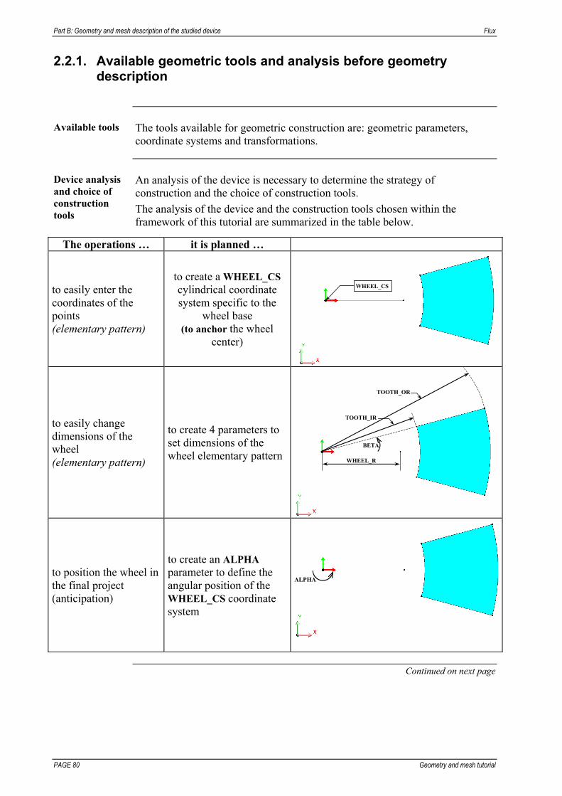
Part B: Geometry and mesh description of the studied device Flux
PAGE 80 Geometry and mesh tutorial
2.2.1. Available geometric tools and analysis before geometry description
Available tools The tools available for geometric construction are: geometric parameters,
coordinate systems and transformations.
Device analysis and choice of construction tools
An analysis of the device is necessary to determine the strategy of construction and the choice of construction tools.
The analysis of the device and the construction tools chosen within the framework of this tutorial are summarized in the table below.
The operations … it is planned …
to easily enter the coordinates of the points (elementary pattern)
to create a WHEEL_CS cylindrical coordinate system specific to the
wheel base (to anchor the wheel
center)
WHEEL_CS
to easily change dimensions of the wheel (elementary pattern)
to create 4 parameters to set dimensions of the wheel elementary pattern
BETA
TOOTH_IR
TOOTH_OR
WHEEL_R
to position the wheel in the final project (anticipation)
to create an ALPHA parameter to define the angular position of the WHEEL_CS coordinate system
ALPHA
Continued on next page
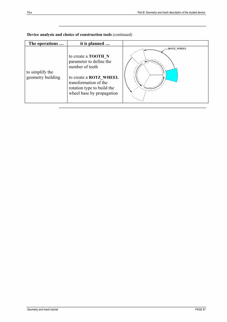
Flux Part B: Geometry and mesh description of the studied device:
Geometry and mesh tutorial PAGE 81
Device analysis and choice of construction tools (continued)
The operations … it is planned …
to simplify the geometry building
to create a TOOTH_N parameter to define the number of teeth to create a ROTZ_WHEEL transformation of the rotation type to build the wheel base by propagation
ROTZ_WHEEL

Part B: Geometry and mesh description of the studied device Flux
PAGE 82 Geometry and mesh tutorial
2.2.2. Main stages for the wheel base geometric description
Outline An outline of the geometry description process to build the wheel base
geometry is presented in the table below.
Caution: the geometric tools will be prepared for building the whole wheel, but we will build only the elementary pattern. The construction of the whole wheel will be carried out with the sensor construction!!!
Stage Description
1 De-activation of Aided mesh
As the WHEEL_BASE.FLU will be later imported in Sensor_2D.FLU it is necessary to de-activate the Aided mesh*
2 Creation of 6 geometric parameters
Tooth inner radius: TOOTH_IR = 12.5 mm Tooth outer radius: TOOTH_OR = 21.5 mm Number of teeth: TOOTH_N = 3 Tooth angle: BETA =15° Wheel radius: WHEEL_R = 10 mm Angle for the wheel angular position
in the final device: ALPHA = 0°
3 Creation of 1 coordinate system
Cylindrical coordinate system: WHEEL_CS (global coordinate system for the wheel description and positioning in the final device)
4 Creation of points and lines for the wheel base
5 Building the face for the wheel base
6 Creation of 1 transformation Rotation transformation for the wheel base: ROTZ_WHEEL
7 The next stages of building the whole wheel by propagation / extrusion will be carried out in the final project (SENSOR_2D.FLU)
* Explanation concerning this subject is presented in § About Aided mesh.

Flux Part B: Geometry and mesh description of the studied device:
Geometry and mesh tutorial PAGE 83
2.3. Creation of geometric tools
Introduction The geometry building begins by the creation of geometric tools: geometric
parameters and a coordinate system.
BETA
TOOTH_IR
TOOTH_OR
WHEEL_RALPHA
WHEEL_CS
Contents This section contains the following topics:
Topic See Page Deactivate aided mesh 84 Create the geometric parameters 85 Create the coordinate system 87

Part B: Geometry and mesh description of the studied device Flux
PAGE 84 Geometry and mesh tutorial
2.3.1. Deactivate aided mesh
Definition Aided mesh is a tool box that permits the user to quickly realize a good
quality mesh. The aided mesh (global adjustment) is activated by default on all flux projects.
Aided mesh and imported Flux project
Aided mesh assigns specific global tool on all entities of a new project. In order not to interfere during project import to the main project, it is needed to de-activate aided mesh on project that will be imported later.
Action To deactivate the Aided mesh, from the Menu:
1. Edit the aided mesh box
2. Select “Inactivated” in the State of aided mesh field
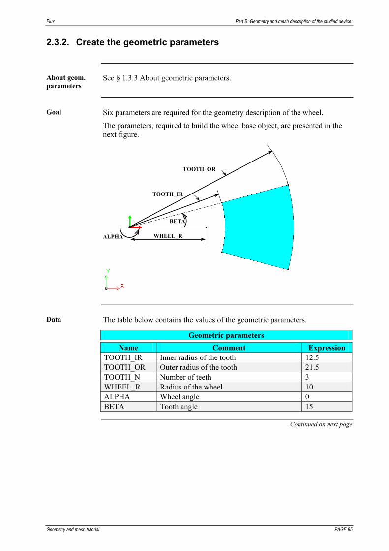
Flux Part B: Geometry and mesh description of the studied device:
Geometry and mesh tutorial PAGE 85
2.3.2. Create the geometric parameters
About geom. parameters
See § 1.3.3 About geometric parameters.
Goal Six parameters are required for the geometry description of the wheel.
The parameters, required to build the wheel base object, are presented in the next figure.
BETA
TOOTH_IR
TOOTH_OR
WHEEL_RALPHA
Data The table below contains the values of the geometric parameters.
Geometric parameters
Name Comment Expression TOOTH_IR Inner radius of the tooth 12.5 TOOTH_OR Outer radius of the tooth 21.5 TOOTH_N Number of teeth 3 WHEEL_R Radius of the wheel 10 ALPHA Wheel angle 0 BETA Tooth angle 15
Continued on next page
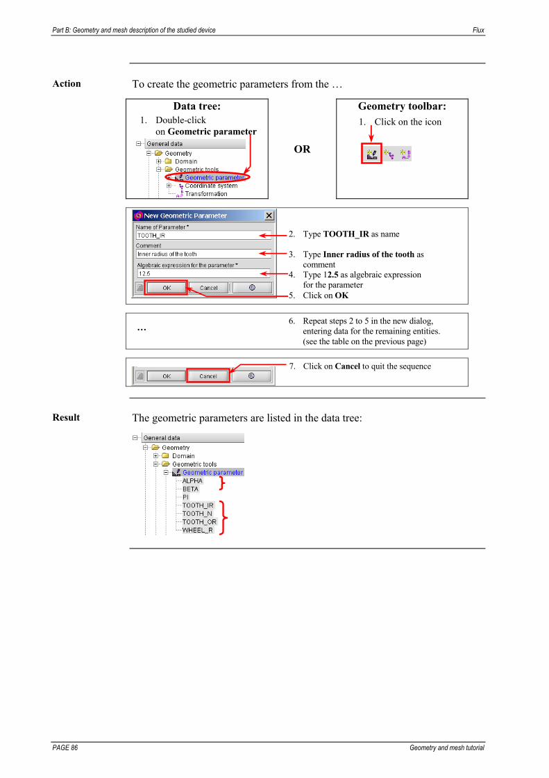
Part B: Geometry and mesh description of the studied device Flux
PAGE 86 Geometry and mesh tutorial
Action To create the geometric parameters from the …
Data tree: 1. Double-click
on Geometric parameter
OR
Geometry toolbar: 1. Click on the icon
2. Type TOOTH_IR as name 3. Type Inner radius of the tooth as
comment 4. Type 12.5 as algebraic expression
for the parameter 5. Click on OK
6. Repeat steps 2 to 5 in the new dialog, entering data for the remaining entities. (see the table on the previous page)
…
7. Click on Cancel to quit the sequence
Result The geometric parameters are listed in the data tree:

Flux Part B: Geometry and mesh description of the studied device:
Geometry and mesh tutorial PAGE 87
2.3.3. Create the coordinate system
About coord.inate systems
See § 1.3.10 About coordinate systems.
Goal A cylindrical coordinate system is required to describe the geometry of the
wheel, as presented in the figure below.
WHEEL_CS
Data The table below describes the coordinate system:
Cylindrical coordinate system type defined with respect to the Global system
Origin coord. Rotation
angle Name Comment Units X Y About Z
WHEEL_CS Wheel coordinate system
millimeter/ degree
0 0 ALPHA
Continued on next page

Part B: Geometry and mesh description of the studied device Flux
PAGE 88 Geometry and mesh tutorial
Action To create the coordinate system from the …
Data tree: 1. Double-click
on Coordinate system
OR
Geometry toolbar: 1. Click on the icon
2. Type WHEEL_CS as name of coordinate system
3. Type Wheel coordinate system as associated comment
4. Select Cylindrical as type of coordinate system
5. Select Global as definition of coordinate system
6. Select MILLIMETER as length unit
7. Select DEGREE as angle unit
8. Type 0 as first coordinate 9. Type 0 as second coordinate
10. Type ALPHA as rotation angle
about Z axis 11. Click on OK
12. Click on Cancel to quit the sequence
Result The coordinate system is listed in the data tree:

Flux Part B: Geometry and mesh description of the studied device:
Geometry and mesh tutorial PAGE 89
2.4. Creation of points and lines for the wheel base
Introduction The next step is the creation of points and lines for the wheel base object.
The next figure describes the geometry of the wheel base object.
BETA
TOOTH_IR
TOOTH_OR
WHEEL_R
Contents This section contains the following topics:
Topic See Page Create the points for the wheel base 90 Create the lines for the wheel base 92

Part B: Geometry and mesh description of the studied device Flux
PAGE 90 Geometry and mesh tutorial
2.4.1. Create the points for the wheel base
About points See § 1.4.1 About points.
Goal Six points are required to build the wheel base outline, as presented in the
figure below.
Point 1
BETA Point 2
Point 3
Point 4
Point 5
Point 6
TOOTH_IR
TOOTH_OR
WHEEL_R
Data The table below describes the points for the wheel base.
Points defined by its parametric coordinates
Coordinates* No
Coordinate system R �
1 0 0 2 WHEEL_R 0 3 TOOTH_IR BETA 4 TOOTH_IR -BETA 5 TOOTH_OR BETA 6
WHEEL_CS
TOOTH_OR -BETA
* Coordinates in cylindrical coordinate system: R, (see § 1.3.10 About coordinate systems).
Continued on next page
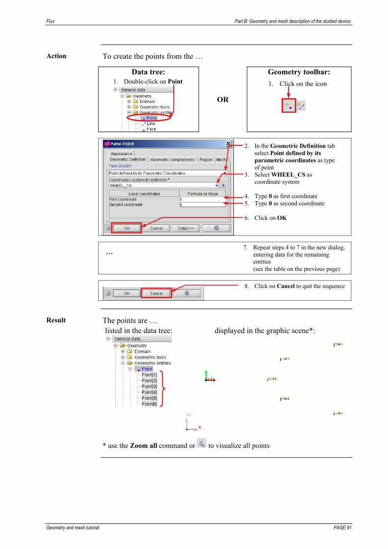
Flux Part B: Geometry and mesh description of the studied device:
Geometry and mesh tutorial PAGE 91
Action To create the points from the …
Data tree: 1. Double-click on Point
OR
Geometry toolbar:
1. Click on the icon
2. In the Geometric Definition tab select Point defined by its parametric coordinates as type of point
3. Select WHEEL_CS as coordinate system
4. Type 0 as first coordinate 5. Type 0 as second coordinate 6. Click on OK
7. Repeat steps 4 to 7 in the new dialog, entering data for the remaining entities (see the table on the previous page)
…
8. Click on Cancel to quit the sequence
Result The points are … listed in the data tree:
displayed in the graphic scene*:
* use the Zoom all command or to visualize all points
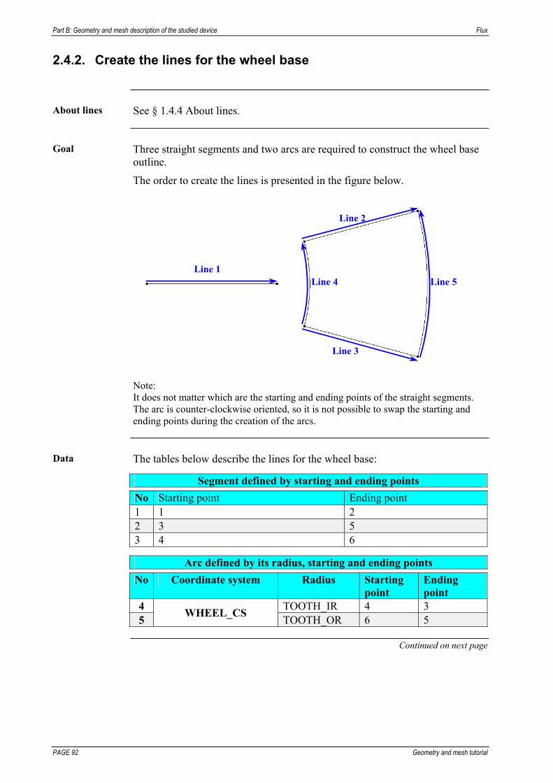
Part B: Geometry and mesh description of the studied device Flux
PAGE 92 Geometry and mesh tutorial
2.4.2. Create the lines for the wheel base
About lines See § 1.4.4 About lines.
Goal Three straight segments and two arcs are required to construct the wheel base
outline.
The order to create the lines is presented in the figure below.
Line 1
Line 2
Line 3
Line 5 Line 4
Note: It does not matter which are the starting and ending points of the straight segments. The arc is counter-clockwise oriented, so it is not possible to swap the starting and ending points during the creation of the arcs.
Data The tables below describe the lines for the wheel base:
Segment defined by starting and ending points
No Starting point Ending point 1 1 2 2 3 5 3 4 6
Arc defined by its radius, starting and ending points
No Coordinate system Radius Starting point
Ending point
4 TOOTH_IR 4 3 5
WHEEL_CS TOOTH_OR 6 5
Continued on next page

Flux Part B: Geometry and mesh description of the studied device:
Geometry and mesh tutorial PAGE 93
Action 1 To create the straight lines from the …
Data tree: 1. Double-click on Line
OR
Geometry toolbar:
1. Click on the icon
2. In the Geometric Definition tab select Segment defined by starting and ending points as type of the line
3. Click on Point 1 in the graphic scene
=> its reference number enters as starting point
4. Click on Point 2 in the graphic scene=> its reference number enters as ending point
5. Repeat steps 3 to 4 in the new reduced dialog to create the remaining segments(see the table on the previous page)
…
6. Click on Cancel to quit the sequence
Result The lines are displayed in the graphic scene:
Continued on next page

Part B: Geometry and mesh description of the studied device Flux
PAGE 94 Geometry and mesh tutorial
Action 2 To create the arcs from the …
Data tree: 1. Double-click on Line
OR
Geometry toolbar:
1. Click on the icon
2. In the Geometric Definition tab select Arc defined by its radius, starting and ending points as type of the line
3. Select WHEEL_CS as coordinate system
4. Type TOOTH_IR as arc radius 5. Click on Point 4 in the graphic scene
=> its reference number enters as starting point
6. Click on Point 3 in the graphic scene=> its reference number enters as ending point
7. Repeat steps 4 to 6 in the new dialog to create the second arc (see the table on page before the previous page)
…
8. Click on Cancel to quit the sequence
Result The lines are … listed in the data tree:
displayed in the graphic scene:

Flux Part B: Geometry and mesh description of the studied device:
Geometry and mesh tutorial PAGE 95
2.5. Building the face for the wheel base
Introduction The next step is building the face for the wheel base object.
Contents This section contains the following topics:
Topic See Page Build the face 96

Part B: Geometry and mesh description of the studied device Flux
PAGE 96 Geometry and mesh tutorial
2.5.1. Build the face
Goal The face will be automatically built by Flux2D.
Action To build the face from the …
Geometry menu: 1. Point on Build and click on Build faces
OR
Geometry toolbar: 1. Click on the icon
Result The face is … listed in the data tree:
displayed in the graphic scene:

Flux Part B: Geometry and mesh description of the studied device:
Geometry and mesh tutorial PAGE 97
2.6. Creation of the transformation
Introduction The whole wheel will be built by means of a transformation. The last step is
the creation of this transformation.
Contents This section contains the following topics:
Topic See Page Create the transformation 98
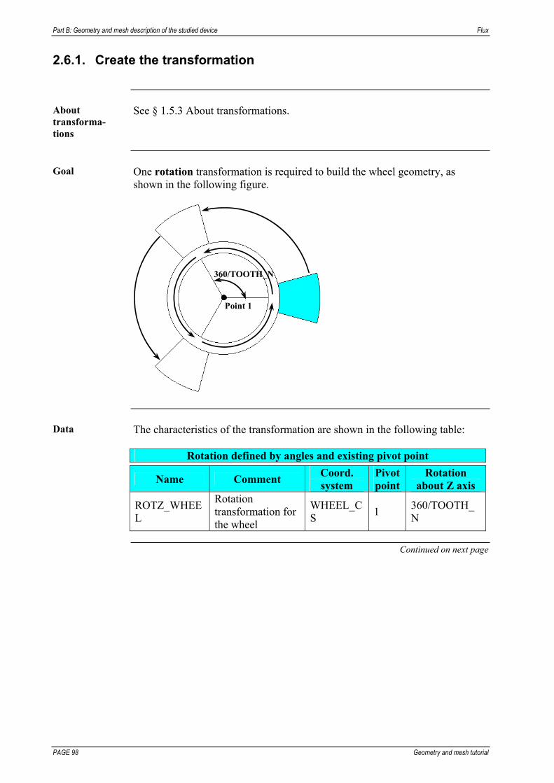
Part B: Geometry and mesh description of the studied device Flux
PAGE 98 Geometry and mesh tutorial
2.6.1. Create the transformation
About transforma-tions
See § 1.5.3 About transformations.
Goal One rotation transformation is required to build the wheel geometry, as
shown in the following figure.
360/TOOTH_N
Point 1
Data The characteristics of the transformation are shown in the following table:
Rotation defined by angles and existing pivot point
Name Comment Coord. system
Pivot point
Rotation about Z axis
ROTZ_WHEEL
Rotation transformation for the wheel
WHEEL_CS
1 360/TOOTH_N
Continued on next page

Flux Part B: Geometry and mesh description of the studied device:
Geometry and mesh tutorial PAGE 99
Action To create the transformations from the …
Data tree: 1. Double-click
on Transformation
OR
Geometry toolbar: 1. Click on the icon
2. Type ROTZ_WHEEL as name 3. Type Rotation transformation
for the wheel as comment 4. Select Rotation defined by
angles and existing pivot point as type
5. Select WHEEL_CS as coordinate system
6. Select point 1 in the list or in the graphic scene as pivot point
7. Type 360/TOOTH_N as rotation angle about Z axis
8. Click on OK
9. Click on Cancel to quit the sequence
Result The transformation is listed in the data tree:

Part B: Geometry and mesh description of the studied device Flux
PAGE 100 Geometry and mesh tutorial

Flux Part B: Geometry and mesh description of the studied device:
Geometry and mesh tutorial PAGE 101
2.6.2. Save and close the project
Goal The current project will be saved and closed.
Action To save and close the project WHEEL_BASE_2D.FLU from the …
Project menu: 1. Click on Close
OR
Project toolbar: 1. Click on the icon
2. Click on Yes
Part B: Geometry and mesh description of the studied device Flux
PAGE 102 Geometry and mesh tutorial

Flux Part B: Geometry and mesh description of the studied device:
Geometry and mesh tutorial PAGE 103
3. Geometric description of the sensor
Introduction This chapter presents the general steps of geometry construction and the data
required to describe the sensor geometry.
The sensor is presented in the figure below.
WHEEL PROBE 1
PROBE 2
INFINITE BOX
Contents This chapter contains the following topics:
Topic See Page Create a Flux project for the sensor 105 Strategy and tools for geometric description of the sensor 107 Importation of the wheel base object and building the whole wheel
111
Importation of the probe objects and positioning of the wheel and probes
125
Completing the domain 131

Part B: Geometry and mesh description of the studied device Flux
PAGE 104 Geometry and mesh tutorial
Flux Part B: Geometry and mesh description of the studied device:
Geometry and mesh tutorial PAGE 105
3.1. Create a Flux project for the sensor
Introduction Each time that a Flux program is started, it is possible to open an existing
project or create a new project.
Contents This section contains the following topics:
Topic See Page
Create and name a new project for the sensor 106
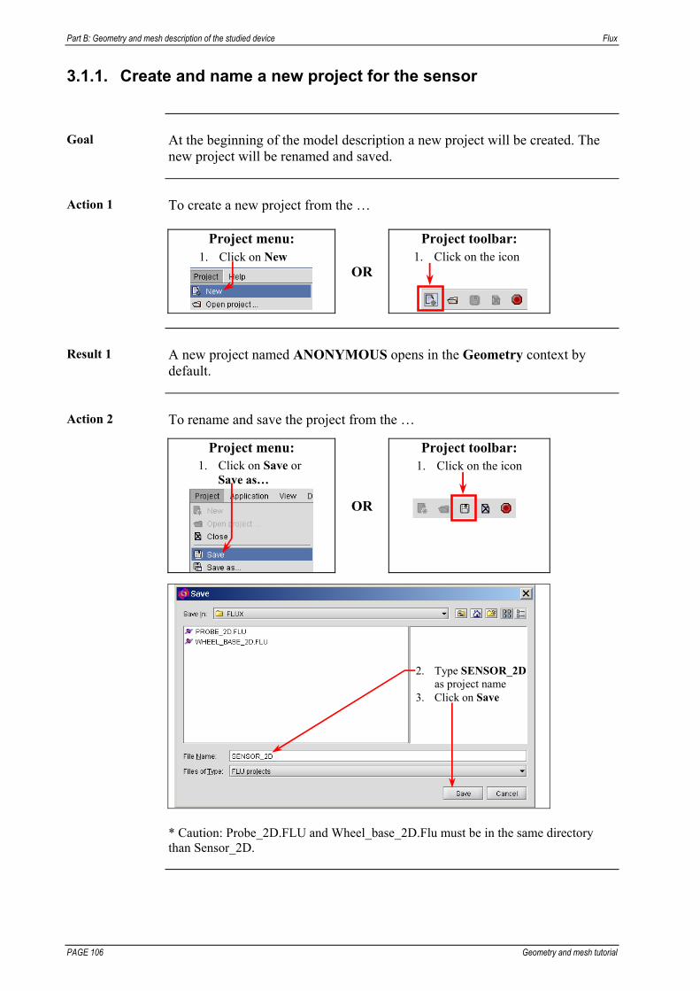
Part B: Geometry and mesh description of the studied device Flux
PAGE 106 Geometry and mesh tutorial
3.1.1. Create and name a new project for the sensor
Goal At the beginning of the model description a new project will be created. The
new project will be renamed and saved.
Action 1 To create a new project from the …
Project menu: 1. Click on New
OR
Project toolbar: 1. Click on the icon
Result 1 A new project named ANONYMOUS opens in the Geometry context by
default.
Action 2 To rename and save the project from the …
Project menu: 1. Click on Save or
Save as…
OR
Project toolbar: 1. Click on the icon
2. Type SENSOR_2D as project name
3. Click on Save
* Caution: Probe_2D.FLU and Wheel_base_2D.Flu must be in the same directory than Sensor_2D.

Flux Part B: Geometry and mesh description of the studied device:
Geometry and mesh tutorial PAGE 107
3.2. Strategy and tools for geometric description of the sensor
Introduction This section shows:
the tools of objects management available in Flux (Flux object importation) the selected strategy for the geometry building of the sensor
Contents This section contains the following topics:
Topic See Page
Available geometric tools and analysis before geometry description
108
Main stages for geometric description 109
Reading advice This section presents an outline of the sensor geometry building process.
Details on the different contents - definition of new concepts, explanation on the use of different tools, etc.- are given in the following sections.

Part B: Geometry and mesh description of the studied device Flux
PAGE 108 Geometry and mesh tutorial
3.2.1. Available geometric tools and analysis before geometry description
Strategy: reminder
The main principle of geometric construction adopted in this tutorial is the following: description of elementary parts of the structure (Flux objects) in
independent Flux projects: probe, base wheel construction of the whole sensor in a new Flux project by using of existing
Flux objects
Device analysis The analysis of the device and the construction tools chosen within the
framework of this tutorial are summarized in the table below.
The operations …
it is planned …
to easily build the wheel base geometry
to use the ROTZ_WHEEL transformation of
rotation type to build the wheel by means of propagation/extrusion
construction
to position the wheel and the probe
to use the ALPHA and ANGLE parameters to rotate the wheel and the probe
ALPHA
ANGLE

Flux Part B: Geometry and mesh description of the studied device:
Geometry and mesh tutorial PAGE 109
3.2.2. Main stages for geometric description
Outline An outline of the geometry description process to build the sensor geometry
is presented in the table below.
Stage Description
1 Importation of the elementary pattern (WHEEL_BASE_3D)
2 Building the whole wheel (see details in § 3.3.2 Geometry building process of the wheel)
3 Importation of a probe object (PROBE_3D)
4 Rotation of the probe and rotation of the cogged wheel
5 Importation of a probe object (PROBE_3D)
6 Addition of an Infinite Box

Part B: Geometry and mesh description of the studied device Flux
PAGE 110 Geometry and mesh tutorial

Flux Part B: Geometry and mesh description of the studied device:
Geometry and mesh tutorial PAGE 111
3.3. Importation of the wheel base object and building the whole wheel
Introduction The geometry description of the sensor begins by the importation of the wheel
base object and building the whole wheel.
The wheel base object and the whole wheel are presented below.
Wheel base Wheel
Contents This section contains the following topics:
Topic See Page
Import the wheel base object 112 Geometry building process of the wheel 113 Propagate the face (tooth) 114 Extrude the line 117 Create an arc 119 Propagate the arc 121 Build faces 123

Part B: Geometry and mesh description of the studied device Flux
PAGE 112 Geometry and mesh tutorial
3.3.1. Import the wheel base object
Goal The wheel base object will be imported into the current project.
Action To import the wheel base object from the Project menu:
1. Point on Import and click on Import FLUX object
2. Click on
3. Select WHEEL_BASE_2D.FLU
4. Click on Open
5. Click on OK
Result The wheel base object is displayed in the graphic scene.
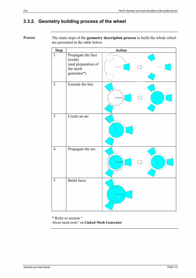
Flux Part B: Geometry and mesh description of the studied device:
Geometry and mesh tutorial PAGE 113
3.3.2. Geometry building process of the wheel
Process The main steps of the geometry description process to build the whole wheel are presented in the table below.
Step Action 1 Propagate the face
(tooth) (and preparation of the mesh generator*)
2 Extrude the line
3 Create an arc
4 Propagate the arc
5 Build faces
* Refer to section “ About mesh tools” on Linked Mesh Generator

Part B: Geometry and mesh description of the studied device Flux
PAGE 114 Geometry and mesh tutorial
3.3.3. Propagate the face (tooth)
About propagation / extrusion
See § 1.5.5 About propagation and extrusion.
Goal The ROTZ_WHEEL transformation will be applied twice to propagate the
face (tooth), as presented in the figure below.
Face 1
Continued on next page

Flux Part B: Geometry and mesh description of the studied device:
Geometry and mesh tutorial PAGE 115
Action To propagate the face from the …
Geometry menu: 1. Point on Propagate
and click on Propagate faces
OR
Geometry toolbar: 1. Click on the icon
2. Select the face in the graphic scene: click on Face 1
=> its reference number enters 3. Select ROTZ_WHEEL as
transformation 4. Type 2 as number of times to apply
the transformation 5. Select Add Faces, Lines and Points
as building options for propagation 6. Click on OK
7. Click on Cancel to quit the sequence
Continued on next page
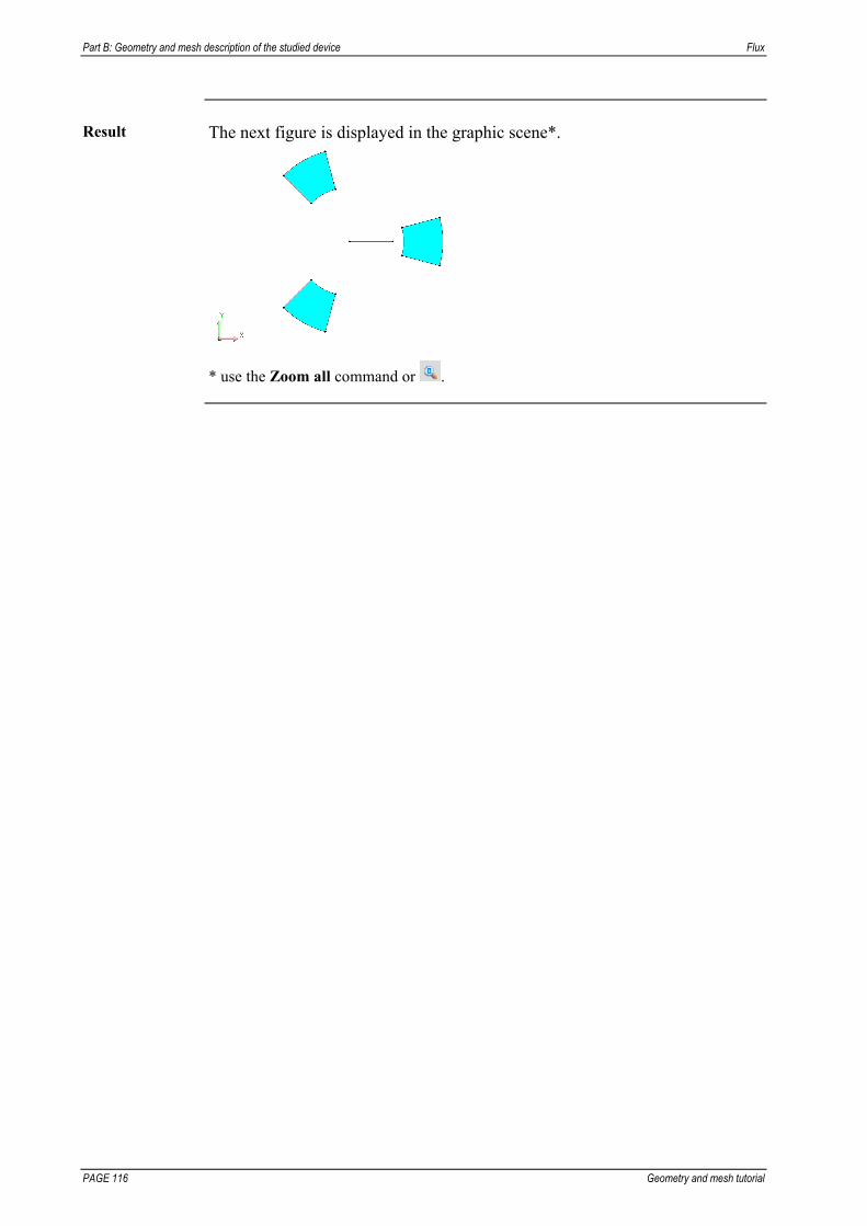
Part B: Geometry and mesh description of the studied device Flux
PAGE 116 Geometry and mesh tutorial
Result The next figure is displayed in the graphic scene*.
* use the Zoom all command or .

Flux Part B: Geometry and mesh description of the studied device:
Geometry and mesh tutorial PAGE 117
3.3.4. Extrude the line
About propagation / extrusion
See § 1.5.5 About propagation and extrusion.
Goal The ROTZ_WHEEL transformation will be applied three times to extrude
the line, as presented in the figure below.
Line 1
Continued on next page

Part B: Geometry and mesh description of the studied device Flux
PAGE 118 Geometry and mesh tutorial
Action To extrude the line from the …
Geometry menu: 1. Point on Extrude and click on Extrude lines
OR
Geometry toolbar: 1. Click on the icon
2. Select the line in the graphic scene:
click on Line 1
=> line reference number enters 3. Select ROTZ_WHEEL as
transformation 4. Type 3 as number of times to apply
the transformation 5. Select Standard as type 6. Select Add Faces, Lines and Points
as building options for extrusion 7. Click on OK
8. Click on Cancel to quit the sequence
Result The next figure is displayed in the graphic scene.

Flux Part B: Geometry and mesh description of the studied device:
Geometry and mesh tutorial PAGE 119
3.3.5. Create an arc
About lines See § 1.4.4 About lines.
Goal One arc is required to connect points 3 and 10 to complete the wheel
geometry, as presented in the figure below.
Point 3
Point 10
Data The table below describes the characteristics of the line to create for the
wheel.
Arc defined by its radius, starting and ending points
No Coordinate system Radius Starting point Ending point 19 WHEEL_CS TOOTH_IR 3 10
Continued on next page

Part B: Geometry and mesh description of the studied device Flux
PAGE 120 Geometry and mesh tutorial
Action To create the line from the …
Data tree: 1. Double-click on Line
OR
Geometry toolbar:
1. Click on the icon
2. In the Geometric Definition tab select Arc defined by its radius, starting and ending points as type of the line
3. Select WHEEL_CS as coordinate system
4. Type TOOTH_IR as arc radius 5. Click on Point 3 in the graphic scene
=> its reference number enters as starting point
6. Click on Point 10 in the graphic scene => its reference number enters as ending point
7. Click on Cancel to quit the sequence
Result The next figure is displayed in the graphic scene.

Flux Part B: Geometry and mesh description of the studied device:
Geometry and mesh tutorial PAGE 121
3.3.6. Propagate the arc
About propagation / extrusion
See § 1.5.5 About propagation and extrusion.
Goal The ROTZ_WHEEL transformation will be applied twice to propagate the
line, as presented in the figure below.
Line 19
Continued on next page

Part B: Geometry and mesh description of the studied device Flux
PAGE 122 Geometry and mesh tutorial
Action To propagate the line from the …
Geometry menu: 1. Point on Propagate
and click on Propagate lines
OR
Geometry toolbar: 1. Click on the icon
2. Select the line in the graphic scene:
click on Line 19
=> its reference number enters 3. Select ROTZ_WHEEL as transformation
4. Type 2 as number of times to apply the transformation
5. Click on OK
6. Click on Cancel to quit the sequence
Result The next figure is displayed in the graphic scene.

Flux Part B: Geometry and mesh description of the studied device:
Geometry and mesh tutorial PAGE 123
3.3.7. Build faces
Goal The faces will be automatically built by Flux2D.
Action To build faces from the …
Geometry menu: 1. Point on Build and click on Build faces
OR
Geometry toolbar: 1. Click on the icon
Result The next figure is displayed in the graphic scene:

Part B: Geometry and mesh description of the studied device Flux
PAGE 124 Geometry and mesh tutorial
Flux Part B: Geometry and mesh description of the studied device:
Geometry and mesh tutorial PAGE 125
3.4. Importation of the probe objects and positioning of the wheel and probes
Introduction The next stages of geometry building are:
the importation of the first probe object, the positioning of the wheel and the first probe by modifying the geometric
parameters the importation of the second probe object
Contents This section contains the following topics:
Topic See Page
Import the first probe object 126 Modify the parameters 128 Import the second probe object 129

Part B: Geometry and mesh description of the studied device Flux
PAGE 126 Geometry and mesh tutorial
3.4.1. Import the first probe object
Goal The probe object will be imported into the current project.
Continued on next page
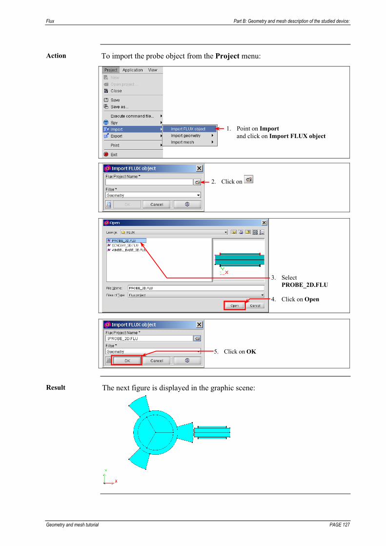
Flux Part B: Geometry and mesh description of the studied device:
Geometry and mesh tutorial PAGE 127
Action To import the probe object from the Project menu:
1. Point on Import and click on Import FLUX object
2. Click on
3. Select PROBE_2D.FLU
4. Click on Open
5. Click on OK
Result The next figure is displayed in the graphic scene:

Part B: Geometry and mesh description of the studied device Flux
PAGE 128 Geometry and mesh tutorial
3.4.2. Modify the parameters
Goal Two geometric parameters will be modified:
ALPHA, corresponding to the angle of the wheel position ANGLE, corresponding to the angle of the probe position
ALPHA
ANGLE
Action To modify the ALPHA and ANGLE parameters from the Data tree:
1. Click on ALPHA and ANGLE
keeping the Ctrl key pressed 2. Right click to open the contextual menu
and click on Edit array
3. Type 75 as ALPHA
expression 4. Type 30 as ANGLE
expression 5. Click on OK
Result The next figure is displayed in the graphic scene:
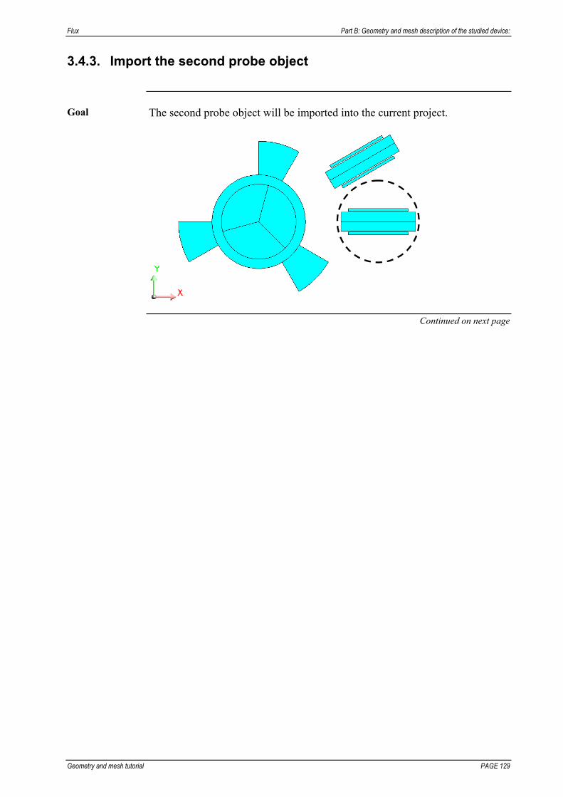
Flux Part B: Geometry and mesh description of the studied device:
Geometry and mesh tutorial PAGE 129
3.4.3. Import the second probe object
Goal The second probe object will be imported into the current project.
Continued on next page

Part B: Geometry and mesh description of the studied device Flux
PAGE 130 Geometry and mesh tutorial
Action To import the probe object from the Project menu:
1. Point on Import and click on Import FLUX object
2. Click on
3. Select PROBE_2D.FLU
4. Click on Open
5. Click on OK
Result The next figure is displayed in the graphic scene:

Flux Part B: Geometry and mesh description of the studied device:
Geometry and mesh tutorial PAGE 131
3.5. Completing the domain
Introduction The last stage of geometry building is adding an infinite box to close the
study domain.
Contents This section contains the following topics:
Topic See Page
About an infinite box 132 Add an infinite box 133 Build faces 134

Part B: Geometry and mesh description of the studied device Flux
PAGE 132 Geometry and mesh tutorial
3.5.1. About an infinite box
Infinite box technique
In the Flux software, using a mathematical transformation to model an infinite domain is called the infinite box technique.
The exterior domain (infinite) is linked to an image domain (called the infinite box) through a space transformation.
Principle of use The use of the infinite box implicitly assumes a null field at infinity.
The boundary conditions on the corresponding boundaries of the infinite box are set automatically in the physical module.
Type of infinite box
The infinite box available for 2D study domain and their characteristics are presented in the table below.
Infinite box Characteristics
disc: centered in (0,0) in the global coordinate
system comprises 8 points, 4 lines dimensions set by the user
Length and angle units
Length and angle units are those associated with the domain.
How to choose the dimensions?
The dimensions of the infinite box are defined by the user. This requires a certain experience because there is no general rule.
We can, however, give some advice: the distance between the device and the interior surface of the infinite box is
at least equal to the dimension of the device in this direction the dimensions of the infinite box are related to the mesh. In Flux 3D, the
number of elements on the thickness of the box must be roughly equal (at least) to two (second-order elements) or to three (first-order elements).
The mesh and the size of the infinite box must take into account the studied phenomena. The computations should be performed as follows: for computing of a global or a local quantity inside the device, it is
unnecessary to refine the mesh of the infinite box; for computing of the field created outside the device, it is necessary to
define the box of more significant size and to refine the mesh inside.
It is recommended to parameterize the dimensions of the infinite box to adjust its size during the meshing.

Flux Part B: Geometry and mesh description of the studied device:
Geometry and mesh tutorial PAGE 133
3.5.2. Add an infinite box
Goal An infinite box will be added to close the study domain.
Data The main characteristics of the infinite box are shown in the following table.
Infinite box of Disc type
Internal radius External radius 60 70
Action To create the infinite box from the …
Data tree: 1. Double-click
on Infinite box
OR
Geometry toolbar: 1. Click on the icon
2. Select Disc as type of the infinite box 3. Type 60 as internal radius 4. Type 70 as external radius
5. Click on OK
Result The infinite box is displayed in the graphic scene:

Part B: Geometry and mesh description of the studied device Flux
PAGE 134 Geometry and mesh tutorial
3.5.3. Build faces
Goal The faces will be automatically built by Flux2D.
Action To build faces from the …
Geometry menu: 1. Point on Build and click on Build faces
OR
Geometry toolbar: 1. Click on the icon
Result The next figure is displayed in the graphic scene.
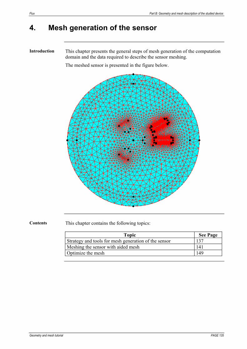
Flux Part B: Geometry and mesh description of the studied device:
Geometry and mesh tutorial PAGE 135
4. Mesh generation of the sensor
Introduction This chapter presents the general steps of mesh generation of the computation
domain and the data required to describe the sensor meshing.
The meshed sensor is presented in the figure below.
Contents This chapter contains the following topics:
Topic See Page Strategy and tools for mesh generation of the sensor 137 Meshing the sensor with aided mesh 141 Optimize the mesh 149

Part B: Geometry and mesh description of the studied device Flux
PAGE 136 Geometry and mesh tutorial

Flux Part B: Geometry and mesh description of the studied device:
Geometry and mesh tutorial PAGE 137
4.1. Strategy and tools for mesh generation of the sensor
Introduction This section shows the available meshing tools and the main stages for mesh
generation of the sensor.
Contents This section contains the following topics:
Topic See Page Available meshing tools and analysis before mesh generation 138 Main stages for mesh description 139

Part B: Geometry and mesh description of the studied device Flux
PAGE 138 Geometry and mesh tutorial
4.1.1. Available meshing tools and analysis before mesh generation
Local / global mesh adjustments
Two solutions are offered to users for the mesh adjustment: the global adjustment (automatic) and / or the local adjustment (manual).
The global adjustment permits to adjust the automatic mesh (triangles elements) of the whole domain taking into account certain geometry constraints (faces or lines that are distorted, thin, or close to each other but that are not part of the same geometry). It is done automatically thanks to the Aided Mesh tool box.
The local adjustment permits to locally adjust the mesh near an entity (point, line) or a group of entities defined by the user (creation and assignment of mesh tools).
Use Usually, it is advised to first mesh the device with the Aided mesh preset
default values. Then if the user is not completely satisfied of the mesh quality, it is possible to adjust the default values of the aided mesh and /or to add some local mesh information where needed.
Device analysis and choice of mesh tools
An analysis of the device is necessary to determine the strategy of meshing, and the choice of mesh tools.
The analysis of the device and the mesh tools chosen within the framework of this tutorial are summarized in the table below.
The operations … it is planned …
to control the node density of the infinite box
to modify 2 predefined mesh
points LARGE and MEDIUM
MEDIUM
LARGE

Flux Part B: Geometry and mesh description of the studied device:
Geometry and mesh tutorial PAGE 139
4.1.2. Main stages for mesh description
Outline An outline of the mesh generating process is presented in the table below.
Stage Description
1 Synchronize with aided mesh preset values 2 Mesh the device
3 Modification of 2 predefined mesh points
Outer size infinite box mesh point: LARGE = 8 mm Inner size infinite box mesh point: MEDIUM = 4 mm
Assignment of the MEDIUM mesh point to points
MEDIUM
4
and assignment of the LARGE mesh point to points
LARGE
5 Creation of a mesh point MAG_MP = 0.5 mm
6
Assignment of the MAG_MP mesh point to the points of the two magnets
MAG_MP
Continued on next page

Part B: Geometry and mesh description of the studied device Flux
PAGE 140 Geometry and mesh tutorial
8 Meshing: meshing lines meshing faces

Flux Part B: Geometry and mesh description of the studied device:
Geometry and mesh tutorial PAGE 141
4.2. Meshing the sensor with aided mesh
Introduction The first step of mesh generation of the sensor is meshing lines and faces with
aided mesh preset values.
Contents This section contains the following topics:
Topic See Page Change to the mesh context 142 About the mesh context 143 About Aided mesh 144 Synchronize Aided mesh value and mesh lines and faces 145

Part B: Geometry and mesh description of the studied device Flux
PAGE 142 Geometry and mesh tutorial
4.2.1. Change to the mesh context
Goal The Geometry context of Flux2D should be changed to the Mesh context.
Action To activate the Mesh context (display the Mesh toolbar) from the Context
toolbar:
1. Select the Mesh Context using the arrows

Flux Part B: Geometry and mesh description of the studied device:
Geometry and mesh tutorial PAGE 143
4.2.2. About the mesh context
Tools of the mesh context
After having activated the Mesh context, toolbars dedicated to the mesh description appear in the Flux2D window.
The different toolbars and their principal roles are briefly described below. 1 2 3 4 5 6
7
Mesh context toolbars Function 1
To edit Aided mesh box
2
to create mesh entities
3 to assign mesh entities to geometric entitiesto clear all mesh information
4
to orient the mesh to structure the mesh
5
to mesh domain, lines and faces
6
to delete the mesh to check the mesh
7
to display mesh points, mesh lines, nodes, surface elements, mesh defects
Part B: Geometry and mesh description of the studied device Flux
PAGE 144 Geometry and mesh tutorial
4.2.3. About Aided mesh
Introduction The global adjustment permits to adjust the automatic mesh (triangles
elements) of the whole domain taking into account certain geometry constraints (faces or lines that are distorted, thin, or close to each other but that are not part of the same geometry). It is done automatically thanks to the Aided Mesh tool box.
Aided mesh The Aided Mesh box groups a list of tools preset with default values that are
available to adjust the mesh globally: Aided mesh point (on free points) Deviation (on free lines/faces) Relaxation (on free line/ faces) The aided mesh is activated by default.
Use Usually, it is advised to first mesh the device with the preset default values.
Then if the user is not completely satisfied of the mesh quality, it is possible to adjust the default values of the aided mesh and /or to add some local mesh information where needed.
Note! If there is global and local adjustment on the same project, the local adjustment has the priority on global adjustment. In this case, the global adjustment information will be assign on entities that are free of local mesh information (free points, free lines and free faces.
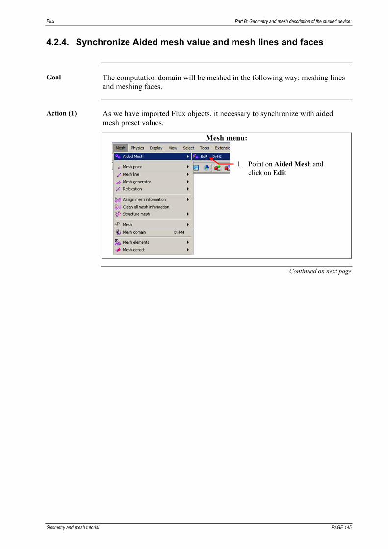
Flux Part B: Geometry and mesh description of the studied device:
Geometry and mesh tutorial PAGE 145
4.2.4. Synchronize Aided mesh value and mesh lines and faces
Goal The computation domain will be meshed in the following way: meshing lines
and meshing faces.
Action (1) As we have imported Flux objects, it necessary to synchronize with aided
mesh preset values.
Mesh menu:
1. Point on Aided Mesh and click on Edit
Continued on next page
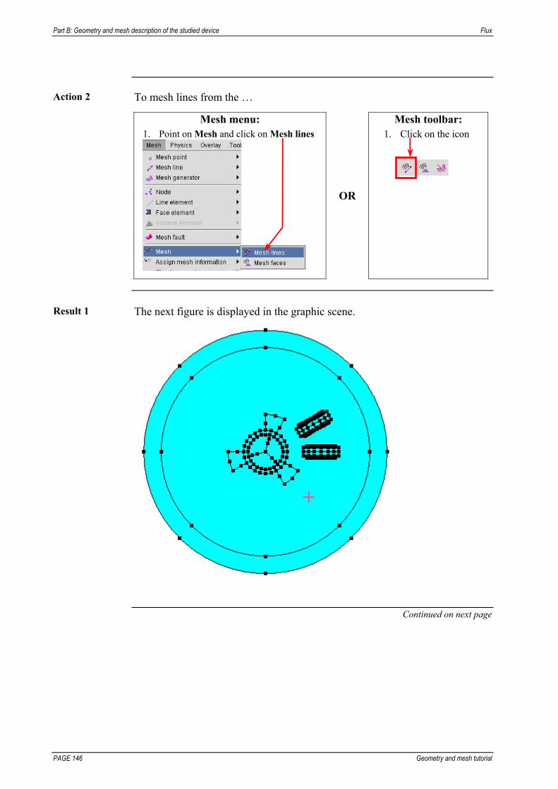
Part B: Geometry and mesh description of the studied device Flux
PAGE 146 Geometry and mesh tutorial
Action 2 To mesh lines from the …
Mesh menu: 1. Point on Mesh and click on Mesh lines
OR
Mesh toolbar: 1. Click on the icon
Result 1 The next figure is displayed in the graphic scene.
Continued on next page

Flux Part B: Geometry and mesh description of the studied device:
Geometry and mesh tutorial PAGE 147
Action 3 To mesh faces from the …
Mesh menu: 1. Point on Mesh and click on Mesh faces
OR
Mesh toolbar: 1. Click on the icon
Result The results appear as below.
The output is displayed in the History zone: Total number of nodes --> 7237
Surface elements : Number of elements not evaluated : 0 % Number of excellent quality elements : 98.28 % Number of good quality elements : 1.64 % Number of average quality elements : 0.08 % Number of poor quality elements : 0 % meshDomain executed
Continued on next page
Part B: Geometry and mesh description of the studied device Flux
PAGE 148 Geometry and mesh tutorial
Comments To optimize the mesh, it is advised to have at least a two elements large
Infinite box and to dense and regularize the mesh in the probes and between the probe and cogged wheel (in order to take into account the physics).

Flux Part B: Geometry and mesh description of the studied device:
Geometry and mesh tutorial PAGE 149
4.3. Optimize the mesh
Introduction After a first mesh, it is necessary to optimize the mesh result by setting aided
values and adding some ‘local” mesh information
Contents This section contains the following topics:
Topic See Page About mesh tools 150 Modify the Aided relaxation on lines and faces 154 Assign mesh points to points 156 Create a mesh point 158 Assign the mesh point to points 159 Create a mesh line 161 Assign meshline to lines 163 Mesh lines and faces 165 Save the project and close the Flux2D window 167

Part B: Geometry and mesh description of the studied device Flux
PAGE 150 Geometry and mesh tutorial

Flux Part B: Geometry and mesh description of the studied device:
Geometry and mesh tutorial PAGE 151
4.3.1. About mesh tools
Mesh To mesh the device is to subdivide the computation domain into finite
elements: nodes line elements face elements volume elements
Meshing tools The meshing tools accessible in the Mesh context are the following:
Tool Function Mesh point to control the size of mesh elements through
the geometric points Mesh line to control the size of mesh elements through
the geometric lines Mesh generator (or algorithms for meshing)
to perform the subdivision into finite elements on faces or volumes
Relaxation to control the repartition of the mesh density through lines, faces and volumes
Shadow To control the mesh in the area where two object are close (only in 3D)
Mesh point The Mesh point distributes nodes on the lines based on weights assigned to
points. The node spacing on a line between two end points with different mesh points is determined by interpolation, taking into consideration the different values at the two ends of the line.
Default mesh points
There are three predefined mesh points: SMALL MEDIUM LARGE
Their values are computed by Flux according to dimensions of the geometry of the device.
The default mesh point values proposed to the user are expressed in millimeters.
Continued on next page

Part B: Geometry and mesh description of the studied device Flux
PAGE 152 Geometry and mesh tutorial
Mesh line The Mesh line distributes nodes on the lines based on a subdivision of the line length.
We can distinguish two modes of distribution of nodes on lines: uniformly distributed nodes: line elements of the same length (uniform
distribution of nodes) nodes distributed in a geometrical progression (non-uniform distribution of
nodes) It is also possible to take into account the node distribution on curved lines with the Mesh line of the deviation type (repartition of nodes in function of a deviation criteria)
Mesh generators
The different mesh generators are the following: generic mesh generators:
- automatic - mapped - none (no mesh)
users mesh generators (associated with a transformation): - linked - extrusion
The automatic mesh generator is used by default in Flux2D.
Mesh generator Function automatic to create triangular elements on the surfaces and
tetrahedral elements on the volumes (option to apply deviation on faces in 3D)
mapped to create quadrangular elements on surfaces and the hexahedral elements on the volumes
none (no mesh) to impose non meshed zones linked to impose the same mesh on faces linked by a geometric
transformation extrusion to reproduce the same mesh in layers on domains
obtained by extrusion (the volume elements are prisms or hexahedrons, depending on the mesh of the base faces)
Continued on next page

Flux Part B: Geometry and mesh description of the studied device:
Geometry and mesh tutorial PAGE 153
Relaxation Relaxation enables the creation of triangular or tetrahedral good quality
elements as big as possible depending of the size of geometrical entity. The mesh is denser on small entities and more relaxed on bigger entities, depending on the relaxation coefficient. The example below show relaxation on lines:
Low relaxation on lines
Medium relaxation on lines
High relaxation on lines
Shadow (3D) Shadow can be applied on faces closed to each other in 3D only. Shadow
enables to take into account the proximity of disconnected objects.

Part B: Geometry and mesh description of the studied device Flux
PAGE 154 Geometry and mesh tutorial
4.3.2. Modify the Aided relaxation on lines and faces
Action Edit the Aided mesh box and modify the relaxation on lines and faces as
below.
1. Edit the Aided mesh box 2. Select Relaxation as parameters of aided
mesh 3. Select Low (r=0.25) as setting of relaxation
for lines 4. Select Low (r=0.25) as setting of relaxation
for faces
5. Click on OK

Flux Part B: Geometry and mesh description of the studied device:
Geometry and mesh tutorial PAGE 155
4.3.3. Modify the mesh points
Goal The LARGE mesh point, applied to the points on the outer lines of the
infinite box, and the MEDIUM mesh point, applied to the points on the inner lines of the infinite box, will be modified.
Data The table below describes the new values for the LARGE and MEDIUM
mesh points.
Mesh points
Name Comment Value Color LARGE Large mesh size 8 Red MEDIUM Medium mesh size 4 Yellow
Action To modify the mesh points from the Data tree:
1. Click on LARGE and MEDIUM, keeping the Ctrl key pressed
2. Right click to open the contextual menu
and click on Edit array
3. Type 8 as
value for the LARGE mesh point
4. Type 4 as value for the MEDIUM mesh point
5. Click on OK

Part B: Geometry and mesh description of the studied device Flux
PAGE 156 Geometry and mesh tutorial
4.3.4. Assign mesh points to points
Goal The mesh points will be assigned to the points on the infinite box as follows:
the MEDIUM mesh point will be assigned to the points on the inner lines
MEDIUM
the LARGE mesh point will be assigned to the points on the outer lines
LARGE
Continued on next page

Flux Part B: Geometry and mesh description of the studied device:
Geometry and mesh tutorial PAGE 157
Action To assign mesh point to points from the …
Mesh menu: 1. Point on Assign mesh information
and click on Assign mesh point to points
OR
Mesh toolbar: 1. Click on the icon
2. Select the points in the graphic scene:
click on the points, keeping the Ctrl key pressed
=> its reference number enters 3. Select MEDIUM as mesh point 4. Click on OK
5. Repeat steps 2 to 4 in the new dialog to assign the LARGE mesh point to points(see the figure on the previous page)
…
6. Click on Cancel to quit the sequence

Part B: Geometry and mesh description of the studied device Flux
PAGE 158 Geometry and mesh tutorial
4.3.5. Create a mesh point
Data The table below describes the characteristics of the mesh points for the probe.
Mesh point
Name Comment Unit Value Color MAG_MP Magnet mesh point millimeter 0.5 White
Action To create the mesh points from the …
Data tree: 1. Double-click on Mesh point
OR
Mesh toolbar: 1. Click on the icon
2. Type MAG_MP as name 3. Type Magnet mesh point as comment 4. In the Definition tab select MILLIMETER
as associated length unit 5. Type 0.5 as value of the mesh point 6. Click on the Appearance tab 7. Select White as color
8. Click on OK
9. Click on Cancel to quit the sequence
Result The new mesh point is listed in the data tree:
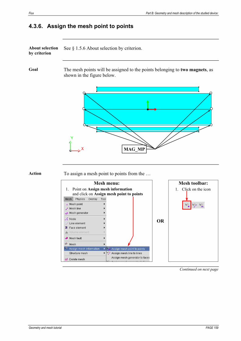
Flux Part B: Geometry and mesh description of the studied device:
Geometry and mesh tutorial PAGE 159
4.3.6. Assign the mesh point to points
About selection by criterion
See § 1.5.6 About selection by criterion.
Goal The mesh points will be assigned to the points belonging to two magnets, as
shown in the figure below.
MAG_MP
Action To assign a mesh point to points from the …
Mesh menu: 1. Point on Assign mesh information
and click on Assign mesh point to points
OR
Mesh toolbar: 1. Click on the icon
Continued on next page
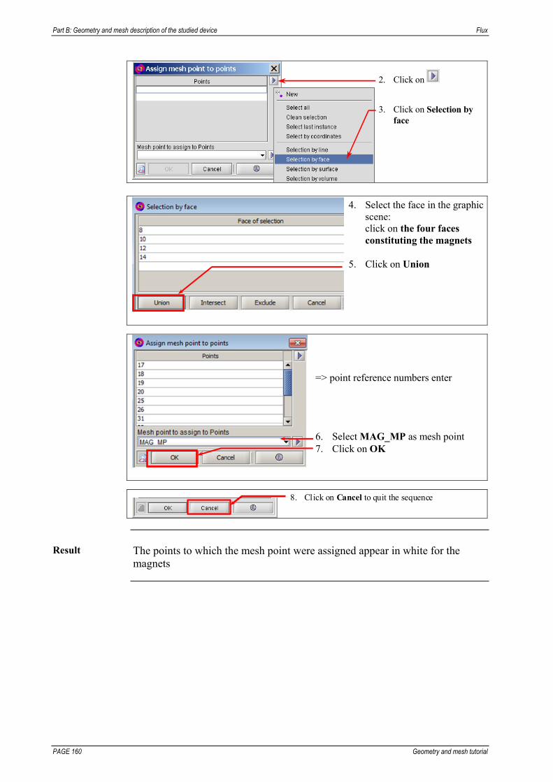
Part B: Geometry and mesh description of the studied device Flux
PAGE 160 Geometry and mesh tutorial
2. Click on 3. Click on Selection by
face
4. Select the face in the graphic scene: click on the four faces constituting the magnets
5. Click on Union
=> point reference numbers enter 6. Select MAG_MP as mesh point 7. Click on OK
8. Click on Cancel to quit the sequence
Result The points to which the mesh point were assigned appear in white for the
magnets

Flux Part B: Geometry and mesh description of the studied device:
Geometry and mesh tutorial PAGE 161
4.3.7. Create a mesh line
Data The table below describes the characteristics of the mesh line for teeth
extremities.
Mesh Line
Name Type Value Color MESHLINE_1 Relative deviation 1.0 White
Action To create the mesh line from the …
Data tree: 1. Double-click on Mesh point
OR
Mesh toolbar:
1. Click on the icon
2. Type Meshline_1 as name 3. In the Definition tab select
Relative deviation 4. Type 1.0 as value of the mesh
point 5. Click on the Appearance tab 6. Select White as color
7. Click on OK
8.
8. Click on Cancel to quit the sequence

Part B: Geometry and mesh description of the studied device Flux
PAGE 162 Geometry and mesh tutorial
Result The new mesh line is listed in the data tree:

Flux Part B: Geometry and mesh description of the studied device:
Geometry and mesh tutorial PAGE 163
4.3.8. Assign meshline to lines
About selection by criterion
See § 1.5.6 About selection by criterion.
Goal The meshline will be assigned to the lines constituting the extremity of the
cogged wheel. The goal is to increase the mesh density in the air gap between the teeth and the magnets when they are in front of each other.
Meshline_1
Action To assign a mesh line to lines from the …
Mesh menu:
1 Point on Assign mesh information and click on Assign meshline to lines
OR Mesh toolbar: 1. Click on the icon
Continued on next page

Part B: Geometry and mesh description of the studied device Flux
PAGE 164 Geometry and mesh tutorial
2. Select the lines in graphic view maintaining Ctrl key pressed
3. Select meshline_1 4. Click OK
9. Click on Cancel to quit the sequence

Flux Part B: Geometry and mesh description of the studied device:
Geometry and mesh tutorial PAGE 165
4.3.9. Mesh lines and faces
Goal The computation domain will be meshed in the following way: meshing lines
and meshing faces.
Action 1 To mesh lines from the …
Mesh menu: 1. Point on Mesh and click on Mesh lines
OR
Mesh toolbar: 1. Click on the icon
Result 1 The next figure is displayed in the graphic scene.
Continued on next page
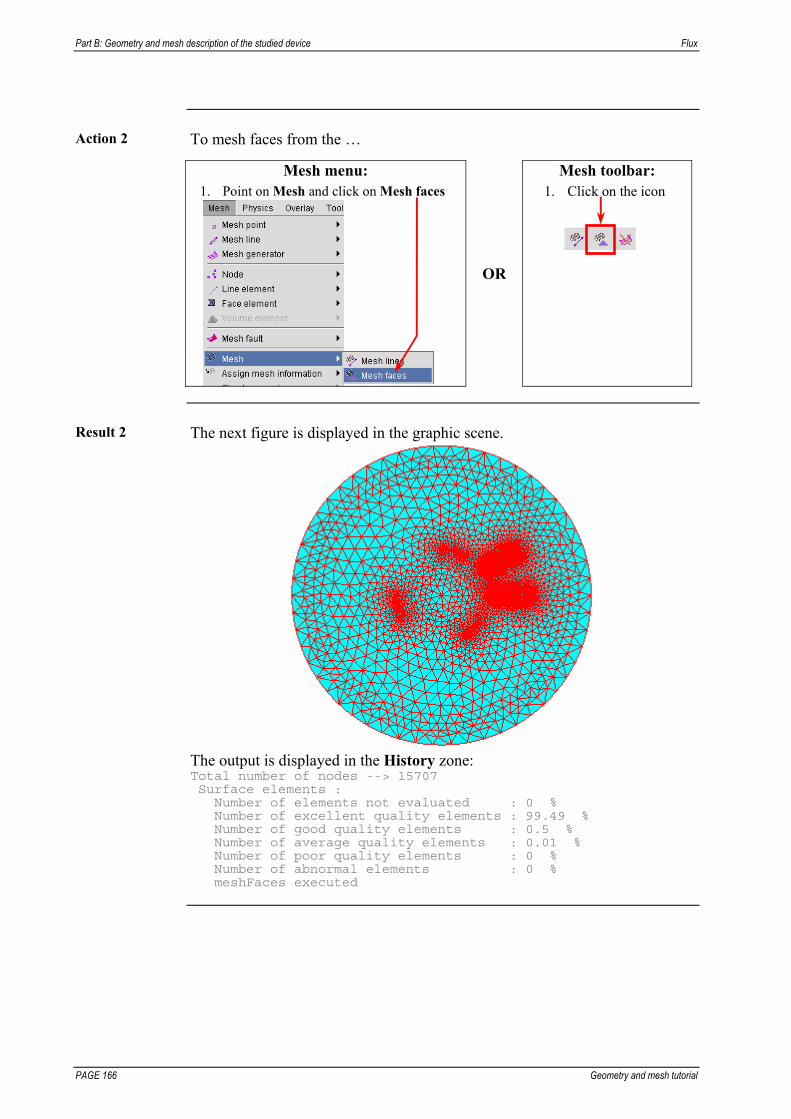
Part B: Geometry and mesh description of the studied device Flux
PAGE 166 Geometry and mesh tutorial
Action 2 To mesh faces from the …
Mesh menu: 1. Point on Mesh and click on Mesh faces
OR
Mesh toolbar: 1. Click on the icon
Result 2 The next figure is displayed in the graphic scene.
The output is displayed in the History zone: Total number of nodes --> 15707
Surface elements : Number of elements not evaluated : 0 % Number of excellent quality elements : 99.49 % Number of good quality elements : 0.5 % Number of average quality elements : 0.01 % Number of poor quality elements : 0 % Number of abnormal elements : 0 % meshFaces executed

Flux Part B: Geometry and mesh description of the studied device:
Geometry and mesh tutorial PAGE 167
4.3.10. Save the project and close the Flux2D window
Goal The current project will be saved and the Flux2D window will be closed to
return to the Flux Supervisor 11.1.
Action 1 To save the SENSOR_2D.FLU project from the …
Project menu: 1. Click on Save
OR
Project toolbar: 1. Click on the icon
Action 2 To close the Flux2D window from the …
Project menu: 1. Click on Exit
OR
Project toolbar: 1. Click on the icon

Part B: Geometry and mesh description of the studied device Flux
PAGE 168 Geometry and mesh tutorial
Flux Part B: Geometry and mesh description of the studied device:
Geometry and mesh tutorial PAGE 169
5. Annex
Introduction This chapter describes the utilization of command files.
Contents This chapter contains the following topics:
Topic See Page Use of command files 171

Part B: Geometry and mesh description of the studied device Flux
PAGE 170 Geometry and mesh tutorial
Flux Part B: Geometry and mesh description of the studied device:
Geometry and mesh tutorial PAGE 171
5.1. Use of command files
Introduction This section describes the use of command files.
Contents This section contains the following topics:
Topic See Page About command files and the Python language 172 Execute command file 173

Part B: Geometry and mesh description of the studied device Flux
PAGE 172 Geometry and mesh tutorial
5.1.1. About command files and the Python language
Introduction Instead of manually executing a series of repetitive actions in Flux, you can
save time by building and executing a command file that performs the task in your place automatically (like a WORD or EXCEL macro).
Command file: definition
A command file is a series of Flux commands and instructions written in the Python language intended to execute a series automatically.
Interest A command file is useful for:
accelerating the most frequent operations combining several commands performing a complex series of tasks

Flux Part B: Geometry and mesh description of the studied device:
Geometry and mesh tutorial PAGE 173
5.1.2. Execute command file
Goal After making a copy of the py file (Flux2D_log.py) of the current project in a
new directory (Tutorial), we will restart the Flux2D window by executing this py file.
Action To execute the py file from the Project menu:
1. Point on Execute command file… and click on Execute command file…
2. Select Preflu2D_log.py
3. Click on Open
vérifier le nom du fichier python…
Result The new files with .FLU extension are recreated in the new directory:
PROBE_2D.FLU WHEEL_BASE_2D.FLU SENSOR_2D.FLU

Part B: Geometry and mesh description of the studied device Flux
PAGE 174 Geometry and mesh tutorial