geometric structure-preserving optimal control …mleok/pdf/blhulesa-jdcs-07.pdf · journal of...
TRANSCRIPT

Journal of Dynamical and Control Systems, Vol. 15, No. 3, July 2009, 307–330 ( c©2009)
GEOMETRIC STRUCTURE-PRESERVING OPTIMALCONTROL OF A RIGID BODY
A. M. BLOCH, I. I. HUSSEIN, M. LEOK, and A. K. SANYAL
Abstract. In this paper, we study a discrete variational optimalcontrol problem for a rigid body. The cost to be minimized is theexternal torque applied to move the rigid body from an initial con-dition to a pre-specified terminal condition. Instead of discretizingthe equations of motion, we use the discrete equations obtained fromthe discrete Lagrange–d’Alembert principle, a process that better ap-
proximates the equations of motion. Within the discrete-time setting,
these two approaches are not equivalent in general. The kinematics
are discretized using a natural Lie-algebraic formulation that guar-
antees that the flow remains on the Lie group SO(3) and its algebraso(3). We use the Lagrange method for constrained problems in thecalculus of variations to derive the discrete-time necessary conditions.We give a numerical example for a three-dimensional rigid body ma-neuver.
1. Introduction
This paper deals with a structure-preserving computational approach tothe optimal control problem of minimizing the control effort necessary toperform an attitude transfer from an initial state to a prescribed final state,in the absence of a potential field. The configuration of the rigid body isgiven by the rotation matrix from the body frame to the spatial frame, whichis an element of the group of orientation-preserving isometries in R
3. Thestate of the rigid body is described by the rotation matrix and its angularvelocity.
To motivate the computational approach we adopt in the discrete-timecase, we first revisit the variational continuous-time optimal control prob-lem. The continuous-time extremal solutions to this optimal control prob-lem have certain special features, since they arise from variational principles.General numerical integration methods, including the popular Runge–Kuttaschemes, typically preserve neither first integrals nor the characteristics of
2000 Mathematics Subject Classification. 37M15, 65K10, 49K15.Key words and phrases. geometric integrators, Lie group integrators, optimal control,
variational methods, rigid body.
307
1079-2724/09/0700-0307/0 c© 2009 Springer Science+Business Media, Inc.
DOI: 10.1007/s10883-00 - -9 9071 2

308 A. M. BLOCH, I. I. HUSSEIN, M. LEOK, and A. K. SANYAL
the configuration space. Geometric integrators are the class of numericalintegration schemes that preserve such properties, and a good survey canbe found in [3]. Techniques particular to Hamiltonian systems are alsodiscussed in [12, 20].
Our approach to discretizing the optimal control problem is in contrast totraditional techniques such as collocation, wherein the continuous equationsof motion are imposed as constraints at a set of collocation points. In ourapproach, modelled after [7], the discrete equations of motion are given by avariational integrator derived from a discrete variational principle [16], andthis induces constraints on the configuration at each discrete time step.
This approach yields discrete dynamics that are more faithful to thecontinuous equations of motion, and consequently yields more accurate so-lutions to the optimal control problem that is being approximated (see [7,Fig. 2]). The geometric structure preservation properties of variational inte-grators in comparison to standard numerical methods, and its implicationsfor the long-time simulation of chaotic rigid body dynamics, are discussedin [10], and a realistic long-time simulation of binary asteroid dynamics isperformed in [22]. These structure preservation properties are extremelyimportant in computing accurate (sub)optimal trajectories for long-termspacecraft attitude maneuvers. For example, in [5], the authors proposean imaging spacecraft formation design that requires a continuous attitudemaneuver over a period of 77 days in a low Earth orbit. Hence, the atti-tude maneuver has to be very accurately computed to meet tight imagingconstraints over long time ranges.
While the discrete optimal control method presented here is illustratedusing the Lie group SO(3) of rotation matrices, and its corresponding Liealgebra so(3) of skew-symmetric matrices, we have derived the method withsufficient generality to address the problem of optimal control on arbitraryLie groups with the drift vector field given by geodesic flow on the group,and it therefore widely applicable. For example, in inter-planetary orbittransfers, one is interested in computing optimal or suboptimal trajectorieson the group of rigid body motions SE(3) with a high degree of accuracy.Similar requirements also apply to the control of quantum systems. Forexample, efficient construction of quantum gates is a problem on the unitaryLie group SU(N). This is an optimal control problem, where one wishes tosteer the identity operator to the desired unitary operator (see, e.g., [9, 19]).
Moreover, an important feature of the way we discretize the optimalcontrol problem is that it is SO(3)-equivariant. The SO(3)-equivarianceof our numerical method is desirable, since it ensures that our results donot depend on the choice of coordinates and coordinate frames. This isin contrast to methods based on coordinatizing the rotation group usingquaternions, (modified) Rodrigues parameters, and Euler angles, as givenin the survey [23]. Even if the optimal cost function is SO(3)-invariant, as in
OPTIMAL CONTROL OF A RIGID BODY 309
[21], the use of generalized coordinates imposes constraints on the attitudekinematics.
For the purpose of numerical simulation, the corresponding discrete op-timal control problem is posed on the discrete state space as a two stagediscrete variational problem. In the first step, we derive the discrete dy-namics for the rigid body in the context of discrete variational mechan-ics [16]. This is achieved by considering the discrete Lagrange–d’Alembertvariational principle [8] in combination with essential ideas from Lie groupmethods [6], which yields a Lie group variational integrator [11] that isa symplectic-momentum integrator that explicitly preserves the Lie groupstructure of the configuration space. These discrete equations are then im-posed as constraints to be satisfied by the extremal solutions to the discreteoptimal control problem, and we obtain the discrete extremal solutions interms of the given terminal states.
The paper is organized as follows. As motivation, in Sec. 2, we studythe minimum control effort optimal control problem in continuous-time. InSec. 3, we study the corresponding discrete-time optimal control problem.In Sec. 3.1 we state the optimal control problem and describe our approach.In Sec. 3.2, we derive the discrete-time equations of motion for the rigid bodystarting with the discrete Lagrange–d’Alembert principle. These equationsare used in Sec. 3.3 to obtain the solution to the discrete optimal controlproblem. In Sec. 4, we describe an algorithm for solving the general non-linear, implicit necessary conditions for SO(3) and give numerical examplesfor rest-to-rest and slew-up spacecraft maneuvers.
2. Continuous-time results
2.1. Problem formulation. In this paper, the natural pairing betweenso∗(3) and so(3) is denoted by 〈·, ·〉. Let 〈〈·, ·〉〉 and 〈〈·, ·〉〉∗ denote the stan-dard (induced by the Killing form) inner product on so(3) and so∗(3), re-spectively. The inner product 〈〈·, ·〉〉∗ is naturally induced from the standardnorm
〈〈ξ,ω〉〉 = −12Tr(ξT ω) ∀ξ,ω ∈ so(3),
through
〈〈η,ϕ〉〉∗ =⟨η,ϕ�
⟩= 〈η,ω〉 =
⟨ξ�,ω
⟩= 〈〈ξ,ω〉〉 , (1)
where ϕ = ω� ∈ so∗(3) and η = ξ� ∈ so∗(3), with ξ,ω ∈ so(3) and � and� are the musical isomorphisms with respect to the standard metric 〈〈·, ·〉〉.On so(3), these isomorphisms correspond to the transpose operation. Thatis, we have ϕ = ωT and η = ξT.
Let J : so(3) → so∗(3) be the positive definite inertia operator. It can beshown that
〈J(ξ),ω〉 = 〈J(ω), ξ〉 . (2)

310 A. M. BLOCH, I. I. HUSSEIN, M. LEOK, and A. K. SANYAL
On so(3), J is given by J(ξ) = Jξ + ξJ , where J is a positive definitesymmetric matrix (see, e.g., [17]). Moreover, we also have
J(η�)� = (JηT + ηTJ)T = J(η),
which is an abuse of notation since η ∈ so∗(3). For the sake of generalityand mathematical precision we will use the general definitions, though ithelps to keep the above identifications for so(3) in mind.
In this section, we review some continuous-time optimal control resultsusing a simple optimal control example on SO(3). The problem we consideris that of minimizing the norm squared of the control torque τ ∈ so∗(3)applied to rotate a rigid body subject to the Lagrange–d’Alembert principlefor the rigid body1 whose configuration is given by R ∈ SO(3) and bodyangular velocity is given by Ω ∈ so(3). We require that the system evolvefrom an initial state (R0,Ω0) to a final state (RT ,ΩT ) at a fixed terminaltime T .
Before proceeding with a statement of the optimal control problem, wefirst define variations of the rigid body configuration R and its velocityΩ. Given a curve R(t) on SO(3), variations of the curve are given byRε(t) := R(t, ε) that satisfies R(t, 0) = R(t). Let W(t) ∈ so(3) be thevariation vector field [1] given by
W(t) = (R(t))−1δR(t),
where
δR(t) =∂Rε(t)
∂ε
∣∣ε=0
∈ TR(t)SO(3).
Since we will be concerned with variations that keep the endpoints fixed, wehave the property that W(0) = 0, W(T ) = 0. The variation in the velocityvector field is denoted by δΩ.
We now state the minimum control effort optimal control problem.
Problem 2.1. Minimize
J =12
T∫
0
〈〈τ , τ 〉〉∗ dt (3)
subject to1. satisfying the Lagrange–d’Alembert principle:
δ
T∫
0
12〈J (Ω) ,Ω〉 dt +
T∫
0
〈τ ,W〉dt = 0, (4)
1This is equivalent to constraining the problem to satisfy the rigid body equations ofmotion given by Eqs. (7). However, for the sake of generality that will be appreciated inthe discrete-time problem, we choose to treat the Lagrange–d’Alembert principle as theconstraint as opposed to the rigid body equations of motion. Both are equivalent in thecontinuous-time case but are generally not equivalent in the discrete-time case.
OPTIMAL CONTROL OF A RIGID BODY 311
for a variation vector field W(t), and subject to R = RΩ,2. and the boundary conditions
R(0) = R0, Ω(0) = Ω0,
R(T ) = RT , Ω(T ) = ΩT .(5)
Now we show that the constraint of satisfying the Lagrange–d’Alembertprinciple leads to the following problem formulation, where the rigid bodyequations of motion replace the Lagrange–d’Alembert principle.
Problem 2.2. Minimize
J =12
T∫
0
〈〈τ , τ 〉〉∗ dt (6)
subject to1. the kinematics and dynamics
R = RΩ, M = ad∗ΩM + τ = [M,Ω] + τ , (7)
where M = J(Ω) ∈ so∗(3) is the momentum,2. and the boundary conditions
R(0) = R0, Ω(0) = Ω0,
R(T ) = RT , Ω(T ) = ΩT .(8)
In the above, ad∗ is the dual of the adjoint representation, ad, of so(3)and is given by ad∗
ξη = −[ξ,η] ∈ so∗(3), for all ξ ∈ so(3) and η ∈ so∗(3).Recall that the bracket is defined by [ξ,ω] = ξω − ωξ.
2.2. The Lagrange–d’Alembert principle and the equations of mo-tion of a rigid body. In this section, we derive the forced rigid bodyequations of motion (Eqs. (7)) from the Lagrange–d’Alembert principle,using a direct derivation based on [17, Sec. 13.5].
First, we take variations of the kinematic condition Ω = R−1R to obtain
δΩ = −R−1 (δR)R−1R + R−1(δR
).
As defined previously, we have
W = R−1δR
and, therefore,
W = −R−1RR−1δR + R−1δR = −ΩW + R−1δR,
sinceδR =
ddt
δR.
Hence, we have
δΩ = −WΩ + ΩW + W = adΩW + W. (9)
312 A. M. BLOCH, I. I. HUSSEIN, M. LEOK, and A. K. SANYAL
Taking variations of the Lagrange–d’Alembert principle we obtainT∫
0
〈J (Ω) , δΩ〉 + 〈τ ,W〉 dt = 0.
Using the variation in Eq. (9) and integrating by parts, we obtain
0 =
T∫
0
⟨−M + ad∗
ΩM + τ ,W⟩
dt + [〈J (Ω) ,W(t)〉]T0 ,
where M = J (Ω) and we used the identity
〈η, adωξ〉 = 〈ad∗ωη, ξ〉 , η ∈ so∗(3), ω, ξ ∈ so(3). (10)
This completes the proof that problem (2.1) is equivalent to problem (2.2).In Sec. 2.3, we demonstrate how the necessary conditions for prob-
lem (2.2) are derived using a variational approach.
2.3. Continuous-time variational optimal control problem. A directvariational approach is used here to obtain the differential equation thatsatisfies the optimal control problem (2.2).
A second-order direct approach. “Second order” is used here toreflect the fact that we now study variations of second order dynamicalequations as opposed to the kinematic direct approach studied in Sec. 2.2.We now give the resulting necessary conditions using a direct approach asin [17]. We already calculate the variations of R and Ω. These were asfollows: δR = RW and δΩ = adΩW+W. We now calculate the variationof M with the goal of obtaining the proper variations for τ :
δM = J(δΩ
)= J
(ddt
δΩ + R (W,Ω)Ω)
,
where R is the curvature tensor on SO(3)(3). The curvature tensor R arisesdue to the identity (see [18, p. 52])
∂
∂ε
∂
∂tY − ∂
∂t
∂
∂εY = R(W,Y)Ω,
where Y ∈ TSO(3) is any vector field along the curve R(t) ∈ SO(3). Takingvariations of M = ad∗
ΩM + τ , we obtain
δM = ad∗δΩM + ad∗
ΩδM + δτ .
We now have the desired variation in τ :
δτ = J (R (W,Ω)Ω) +ddt
J (δΩ) − ad∗δΩM − ad∗
ΩδM. (11)
Taking variations of the cost functional (6) we obtain:
OPTIMAL CONTROL OF A RIGID BODY 313
δJ =
T∫
0
(⟨J(ς) − ad∗
Ω (J(ς)) + η − ddt
(ad∗
ςM)
+[R (
J(ς)�,Ω)Ω]�
+ ad∗Ωad∗
ςM − ad∗Ωη,W
⟩)dt,
where ς = τ � ∈ so(3) and η = J (adΩς) ∈ so∗(3). In obtaining the aboveexpression, we have used integration by parts and the boundary conditions(8), Eqs. (9) and (11), and identities (1), (2), and (10). Hence, we have thefollowing theorem.
Theorem 2.1. The necessary optimality conditions for the problem ofminimizing (6) subject to the dynamics (7) and the boundary conditions (8)are given by the single fourth-order2 differential equation
0 = J(ς) − ad∗Ω (J(ς)) + η − d
dt
(ad∗
ςM)
+[R((J(ς))�
,Ω)Ω]�
+ ad∗Ω
(ad∗
ςM)− ad∗
Ωη,
as well as Eqs. (7) and the boundary conditions (8), where ς and η are asdefined above.
Note that for a compact semi-simple Lie group G with Lie algebra g, thecurvature tensor, with respect to a bi-invariant metric, is given by (see [18]):
R (X,Y)Z =14adadXYZ, (12)
for all X,Y,Z ∈ g.
Remark 2.1. Note that the equations of motion that arise from theLagrange–d’Alembert principle are used to define the dynamic constraints.So, in effect, we are minimizing J subject to satisfying the Lagrange–d’Alembert principle for the rigid body. Analogously, the discrete versionof the Lagrange–d’Alembert principle will be used to derive the discreteequations of motion in the discrete optimal control problem to be studiedin Sec. 3.3. This view is in line with the approach in [7] in that we do notdiscretize the equations of motion directly, but, instead, we discretize theLagrange–d’Alembert principle. These two approaches are not equivalentin general.
3. Discrete-time results
3.1. Problem formulation. In this section, we give the discrete versionof the problem introduced in Sec. 2.1. So, we consider minimizing thenorm squared of the control torque τ subject to satisfaction of the discrete
2Second order in τ and fourth order in R.
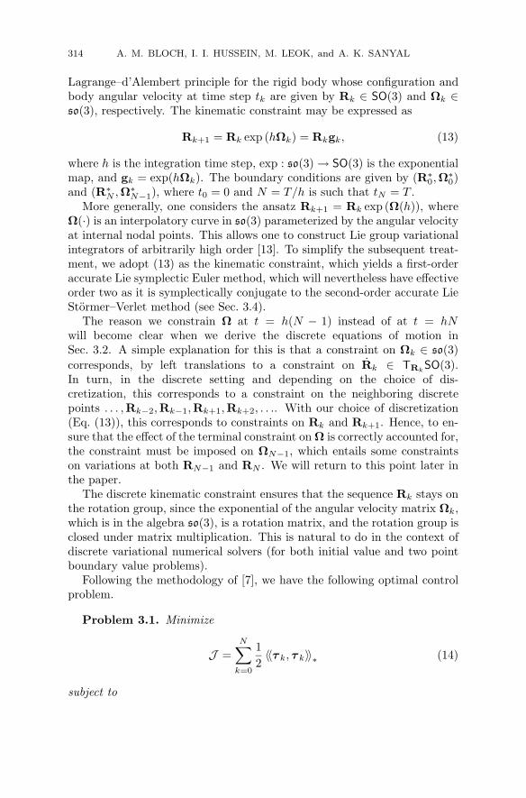
314 A. M. BLOCH, I. I. HUSSEIN, M. LEOK, and A. K. SANYAL
Lagrange–d’Alembert principle for the rigid body whose configuration andbody angular velocity at time step tk are given by Rk ∈ SO(3) and Ωk ∈so(3), respectively. The kinematic constraint may be expressed as
Rk+1 = Rk exp (hΩk) = Rkgk, (13)
where h is the integration time step, exp : so(3) → SO(3) is the exponentialmap, and gk = exp(hΩk). The boundary conditions are given by (R∗
0,Ω∗0)
and (R∗N ,Ω∗
N−1), where t0 = 0 and N = T/h is such that tN = T .More generally, one considers the ansatz Rk+1 = Rk exp (Ω(h)), where
Ω(·) is an interpolatory curve in so(3) parameterized by the angular velocityat internal nodal points. This allows one to construct Lie group variationalintegrators of arbitrarily high order [13]. To simplify the subsequent treat-ment, we adopt (13) as the kinematic constraint, which yields a first-orderaccurate Lie symplectic Euler method, which will nevertheless have effectiveorder two as it is symplectically conjugate to the second-order accurate LieStormer–Verlet method (see Sec. 3.4).
The reason we constrain Ω at t = h(N − 1) instead of at t = hNwill become clear when we derive the discrete equations of motion inSec. 3.2. A simple explanation for this is that a constraint on Ωk ∈ so(3)corresponds, by left translations to a constraint on Rk ∈ TRk
SO(3).In turn, in the discrete setting and depending on the choice of dis-cretization, this corresponds to a constraint on the neighboring discretepoints . . . ,Rk−2,Rk−1,Rk+1,Rk+2, . . .. With our choice of discretization(Eq. (13)), this corresponds to constraints on Rk and Rk+1. Hence, to en-sure that the effect of the terminal constraint on Ω is correctly accounted for,the constraint must be imposed on ΩN−1, which entails some constraintson variations at both RN−1 and RN . We will return to this point later inthe paper.
The discrete kinematic constraint ensures that the sequence Rk stays onthe rotation group, since the exponential of the angular velocity matrix Ωk,which is in the algebra so(3), is a rotation matrix, and the rotation group isclosed under matrix multiplication. This is natural to do in the context ofdiscrete variational numerical solvers (for both initial value and two pointboundary value problems).
Following the methodology of [7], we have the following optimal controlproblem.
Problem 3.1. Minimize
J =N∑
k=0
12〈〈τ k, τ k〉〉∗ (14)
subject to

OPTIMAL CONTROL OF A RIGID BODY 315
1. satisfying the discrete Lagrange–d’Alembert principle:
δ
N−1∑
k=0
12〈J (Ωk) ,Ωk〉 +
N∑
k=0
〈τ k,Wk〉 = 0, (15)
subject to R0 = R∗0, RN = R∗
N and Rk+1 = Rkgk, k = 0, 1, . . . , N−1,where Wk is the variation vector field at time step tk satisfying δRk =RkWk,
2. and the boundary conditions
R0 = R∗0, Ω0 = Ω∗
0,
RN = R∗N , ΩN−1 = Ω∗
N−1.(16)
In problem (3.1), the discrete Lagrange–d’Alembert principle is used toderive the equations of motion for the rigid body with initial and terminalconfiguration constraints. Hence, we get a two point boundary value prob-lem. The full configuration and velocity boundary conditions come into thepicture when we study the optimal control problem. We will show that theconstraint of satisfying the Lagrange–d’Alembert principle in problem (3.1)leads to the following problem formulation, where the discrete rigid bodyequations of motion replace the Lagrange–d’Alembert principle constraint.Only when addressing the following optimal control problem will we needto include the velocity boundary conditions in the derivation.
Problem 3.2. Minimize
J =N∑
k=0
12〈〈τ k, τ k〉〉∗ (17)
subject to1. the discrete kinematics and dynamics
Rk+1 = Rkgk, k = 0, . . . , N − 1,
Mk = Ad∗gk
(hτ k + Mk−1) , k = 1, . . . , N − 1,
Mk = J (Ωk) , k = 0, . . . , N − 1,
(18)
2. and the boundary conditions
R0 = R∗0, Ω0 = Ω∗
0,
RN = R∗N , ΩN−1 = Ω∗
N−1.(19)
Regarding terminal velocity conditions, note that in the second of equa-tions (18) if we let k = N we find that ΩN appears in the equation. Aconstraint on ΩN dictates constraints at the points RN and RN+1 throughthe first equation in (18). Since we only consider time points up to t = Nh,we cannot allow k = N in the second of equations (18) and hence ourterminal velocity constraints are posed in terms of ΩN−1 instead of ΩN .

316 A. M. BLOCH, I. I. HUSSEIN, M. LEOK, and A. K. SANYAL
As mentioned above, Wk is a variation vector field associated with theperturbed group element Rε
k. Likewise, we need to define a variation vectorfield associated with the element gk = exp(hΩk). First, let the perturbedvariable gε
k be defined by
gεk = gk exp(εhδΩk), (20)
where
δΩk =∂Ωε
k
∂ε
∣∣∣∣ε=0
.
Note that gεk
∣∣ε=0
= gk as desired. Moreover, we have
δgk = gk(hδΩk) exp(εhδΩk)∣∣ε=0
= hgkδΩk. (21)
This will be needed later when taking variations.
3.2. The discrete Lagrange–d’Alembert principle and the equa-tions of motion of a rigid body. In this section, we derive the discreteforced rigid body equations of motion (18) from the discrete Lagrange–d’Alembert principle.
We begin by computing the constrained variation associated with thekinematic constraint (13). Taking variations of the kinematic constraint,we obtain
−R−1k (δRk)R−1
k Rk+1 + R−1k δRk+1 = hgk · δΩk,
which is equivalent to
−Wkgk + gkWk+1 = hgkδΩk,
or
δΩk =1h
[−Adg−1
kWk + Wk+1
]. (22)
Note that this is an expression over the Lie algebra so(3).After simple algebraic and re-indexing operations, the Lagrange–
d’Alembert principle gives
0 =⟨
τ 0 − 1h
Ad∗g−10
J (Ω0) ,W0
⟩+⟨
τN +1hJ (ΩN−1) ,WN
⟩
+N−1∑
k=1
⟨τ k − 1
hAd∗
g−1k
J (Ωk) +1hJ (Ωk−1) ,Wk
⟩.
where we have used Eq. (22). By the boundary conditions R0 = R∗0 and
RN = R∗N , we have W0 = 0 and WN = 0. Since δΩk, k = 0, . . . , N−1, and
Wk, k = 1, . . . , N − 1, are arbitrary and independent, then the Lagrange–d’Alembert principle requires that Eqs. (18) hold. The variables Mk, k =0, . . . , N − 1, are of course nothing but the discrete angular momentum ofthe rigid body.

OPTIMAL CONTROL OF A RIGID BODY 317
Equations (18) can be viewed in two ways. The first is to consider thetwo point boundary value problem where we retain the terminal conditionon RN . In this case a (constrained) variety of a combination of controltorques τ k, k = 0, . . . , N , and initial velocity conditions Ω0 can be chosento drive the rigid body from the initial condition R0 to the terminal con-dition RN . The second view is to treat it as an initial value problem byignoring any terminal configuration constraints. In this case WN �= 0 andany combination of control torques τ k, k = 0, . . . , N , and initial velocityconditions Ω0 can be chosen freely.
Simulation results. To test our results, we re-write the discrete equations(18) for the subgroup SO(2). For SO(2) we have
Rk =[
cos θk − sin θk
sin θk cos θk
], Ωk =
[0 −ωk
ωk 0
](23)
and
exp (Ωk) =[
cos ωk − sin ωk
sin ωk cos ωk
]. (24)
The inertia operation is simply given by
J (Ωk) =[
0 −Iωk
Iωk 0
], (25)
where I is the mass moment of inertia of the body about the out-of-planeaxis. One can verify that Adexp(ω)ξ = ξ and that Ad∗
exp(ω)η = η, for allξ,ω ∈ so(2) and η ∈ so∗(2).
Then Eqs. (18) (treated as an initial-value problem) are given for SO(2)by
θk+1 = θk + hωk, k = 0, . . . , N − 1,
ωk =h
Iτk + ωk−1, k = 1, . . . , N − 1,
(26)
in addition to the initial conditions θ0 = θ∗0 , ω0 = ω∗0 .
To verify the accuracy of our numerical computation, we give the corre-sponding continuous-time equations of motion for the planar rigid body onSO(2) using Eqs. (7). The Lie bracket on SO(2) is identically equal to zero.Hence, one can check that Eqs. (7) are given by θ = ω and ω = τ/I, whereθ, ω, and τ are the continuous time angular position, velocity, and torque,respectively. We integrate the equations using the torque τ(t) = sin (πt/2),t ∈ [0, T ]. We use the following parameters for our simulations: T = 10,I = 1, θ(0) = 3, ω(0) = 4, and we try three different time steps correspond-ing to N = 1000, 1500, and 2000. The error between the continuous- anddiscrete-time values of θ and ω are given in Fig. 1. Note that the accuracyof the simulation improves with increasing N .

318 A. M. BLOCH, I. I. HUSSEIN, M. LEOK, and A. K. SANYAL
Fig. 1. Error dynamics on SO(2).
Remark 3.1. Note that the discrete-time equations (26) correspond tothe Euler approximation for the equations of motion. This is a check thatour method returns something familiar for a simple example as the planarrigid body. However, we emphasize that on SO(3) the discretization will notnecessarily be equivalent to any of the classical discretization schemes. The

OPTIMAL CONTROL OF A RIGID BODY 319
discretization will generally result in a set of nonlinear implicit algebraicequations.
3.3. Discrete-time variational optimal control problem. We now ad-dress problem (3.2) by computing the constrained variation δτ k arising fromthe discrete equations of motion. Using Eq. (22) and taking the variationof the second equation in (18), we obtain
δτ k = Ad∗g−1
k
(1h2
J(Wk+1 − Adg−1
kWk
)
+1h
[Wk+1 − Adg−1
kWk,J (Ωk)
])
− 1h2
J(Wk − Adg−1
k−1Wk−1
), (27)
for k = 1, . . . , N − 1. Taking variations of the cost functional (17) andsubstituting from Eq. (27) one obtains after a tedious but straight forwardcomputation an expression for δJ in terms of δτ k:
δJ =N−1∑
k=1
[⟨Ad∗
g−1k
(1h2
J(Wk+1 − Adg−1
kWk
)
+1h
[Wk+1 − Adg−1
kWk,J (Ωk)
])− 1
h2J(Wk − Adg−1
k−1Wk−1
), τ �
k
⟩]
+⟨δτ 0, τ
�0
⟩+⟨δτN , τ �
N
⟩.
When δJ is equated to zero (and after some algebraic rearrangement), onecan obtain the boundary conditions on τ 0, τ 1, τN−1, τN from the resultingequations below:
τ 0 = 0,
0 = − 1h2
(J(τ �
1
)+ Ad∗
g−11
J(Adg−1
1τ �
1
))
− 1h
Ad∗g−11
[J (Ω1) ,Adg−1
1
(τ �
1
)],
0 = − 1h2
(J(τ �
N−1
)+ Ad∗
g−1N−1
J(Adg−1
N−1τ �
N−1
))
− 1h
Ad∗g−1
N−1
[J (ΩN−1) ,Adg−1
N−1
(τ �
N−1
)],
τN = 0
as well as discrete evolution equations that are written in algebraic nonlinearform as follows:
0 = − 1h2
(J(τ �
k
)− Ad∗
g−1k
J(τ �
k+1
)− J
(Adg−1
k−1τ �
k−1
)

320 A. M. BLOCH, I. I. HUSSEIN, M. LEOK, and A. K. SANYAL
+ Ad∗g−1
kJ(Adg−1
kτ �
k
))− 1
h
(Ad∗
g−1k
[J (Ωk) ,Adg−1
k
(τ �
k
)]
− 1h
[J (Ωk−1) ,Adg−1
k−1
(τ �
k−1
)]), (28)
for k = 2, . . . , N − 2.This result is summarized in the following theorem.
Theorem 3.1. The necessary optimality conditions for the discreteproblem (3.2) are
Rk+1 = Rkgk, k = 1, . . . , N − 2,
Mk = Ad∗gk
(hτ k + Mk−1) , k = 1, . . . , N − 1,
0 = − 1h2
(J(τ �
k
)− Ad∗
g−1k
J(τ �
k+1
)
− J(Adg−1
k−1τ �
k−1
)+ Ad∗
g−1k
J(Adg−1
kτ �
k
))
− 1h
(Ad∗
g−1k
[J (Ωk) ,Adg−1
k
(τ �
k
)]
− 1h
[J (Ωk−1) ,Adg−1
k−1
(τ �
k−1
)]), k = 2, . . . , N − 2,
Mk = J (Ωk) , k = 0, . . . , N − 1,
and the boundary conditions
R0 = R∗0, R1 = R∗
0g∗0, Ω0 = Ω∗
0,
RN = R∗N , RN−1 = R∗
N
(g∗
N−1
)−1, ΩN−1 = Ω∗
N−1,
τ 0 = 0, τN = 0,
where g∗0 = exp(hΩ∗
0) and g∗N−1 = exp
(hΩ∗
N−1
).
The following discussion shows that while our discrete approximation(13) is formally first-order accurate, it is symplectically equivalent to thesecond-order accurate Stormer–Verlet method, and hence has effective ordertwo.
3.4. Lie symplectic Euler and symplectic Equivalence. Note thatthe discrete Lagrangian adopted in our paper is obtained by approximatingthe velocity as a constant over the time step h, and by approximating theintegral in time by
t2∫
t1
f(t)dt ≈ (t2 − t1)f(t1).

OPTIMAL CONTROL OF A RIGID BODY 321
In the Lie group setting, the constant angular velocity approximation cor-responds to the condition,
Rk+1 = Rk exp(hΩk)
or, equivalently,
Ωk =1h
exp−1(R−1k Rk+1).
If we set G = Rn and we introduce the notation (q,v) ∈ TR
n, we obtain
vk =qk+1 − qk
h,
which is a usual finite-difference approximation for the velocity. Considerthen a Lagrangian of the form
L(q,v) =12vT Mv − V (q).
Approximating the action integral from 0 to h using a constant velocityapproximation and a quadrature formula, we have
h∫
0
L(q(t),v(t))dt ≈h∫
0
L(q(t),
qk+1 − qk
h
)dt ≈ hL
(qk,
qk+1 − qk
h
).
We then consider choose the discrete Lagrangian
Ld(qk,qk+1) = hL(qk,
qk+1 − qk
h
)
= h
[12
(qk+1 − qk
h
)T
M(qk+1 − qk
h
)− V (qk)
].
The discrete Euler–Lagrange equations
D2Ld(qk−1,qk) + D1Ld(qk,qk+1) = 0
yield
M(qk − qk−1
h
)− M
(qk+1 − qk
h
)− h
∂V
∂q(qk) = 0,
which induces an implicit update map (qk−1,qk) → (qk,qk+1). To obtainthe corresponding Hamiltonian update map, we push-forward this algorithmto T ∗Q by using the discrete fiber derivative FLd : Q × Q → T ∗Q, whichtakes (qk,qk+1) → (qk+1,D2Ld(qk,qk+1)). In particular, we have
pk+1 = D2Ld(qk,qk+1) = M(qk+1 − qk
h
),
which impliesqk+1 = qk + hM−1pk+1. (29)
This allows us to rewrite the discrete Euler–Lagrange equations as follows:
pk − pk+1 − h∂V
∂q(qk) = 0

322 A. M. BLOCH, I. I. HUSSEIN, M. LEOK, and A. K. SANYAL
or, equivalently,
pk+1 = pk − h∂V
∂q(qk). (30)
Now (29) and (30) are precisely the symplectic Euler method applied to thecorresponding Hamiltonian vector field, as we shall see.
The corresponding Hamiltonian is given by
H(q,p) =12pT M−1p + V (q).
The Hamilton equations yield
(qp
)=
⎛
⎜⎜⎝
∂H
∂p
−∂H
∂q
⎞
⎟⎟⎠ =
⎛
⎜⎝
M−1p
−∂V
∂q
⎞
⎟⎠ .
The symplectic Euler method has the form
qk+1 = qk + hq(qk,pk+1),
pk+1 = pk + hp(qk,pk+1),
which yields
qk+1 = qk + hM−1pk+1,
pk+1 = pk + h
(−∂V
∂q(qk)
),
which is precisely what we obtained in (29) and (30). This demonstratesthat our method is the generalization of the symplectic Euler method toLie groups, which has important numerical consequences. While symplecticEuler is formally first-order accurate, it is symplectically equivalent [24,14] to the second-order accurate Stormer–Verlet method [4]. This meansthat one can obtain the Stormer–Verlet method FSV by conjugating thesymplectic Euler method FE with a symplectic transformation T ,
FSV = TFET−1.
In particular, numerical trajectories of symplectic Euler will shadow numer-ical trajectories obtained using Stormer–Verlet. Consider the implicationsof this symplectic equivalence for our discrete optimal control problem. Letthe boundary conditions be specified by q0,qN , and assume that we useStormer–Verlet to propagate the solution, then the boundary condition isexpressed as
qN = FNSVq0 = (TFET−1)Nq0 = TFN
E T−1q0,
which is equivalent to
qN = T−1qN = FNE T−1q0 = FN
E q0.

OPTIMAL CONTROL OF A RIGID BODY 323
This implies that if we preprocess the boundary conditions q0 and qN toobtain q0 = T−1q0 and qN = T−1qN , we can use symplectic Euler at theinternal stages to propagate the states and costates, and then postprocessthem to obtain the trajectory one would have obtained by using Stormer–Verlet.
In practice, the shadowing result imparts the symplectic Euler methodwith the same desirable qualitative properties as Stormer–Verlet, and itis not necessary to postprocess the numerical solutions in order to achieveaccurate results. Since on an appropriate choice of charts, our Lie symplecticEuler method reduces to symplectic Euler in coordinates, it follows thatthere is a corresponding second-order Lie Stormer–Verlet method that ourmethod is symplectically equivalent to, and in particular, our method haseffective order two.
4. Numerical approach and results
The first-order optimality equations, Eq. (28), in combination with theboundary conditions,
R0 = R∗0, RN = R∗
N , Ω0 = Ω∗0, ΩN−1 = Ω∗
N−1,
leave the torques τ 1, . . . , τN−1, and the angular velocities Ω1, . . . ,ΩN−2 asunknowns. By substituting the relations gk = exp(hΩk), Mk = J(Ωk), wecan rewrite the necessary conditions (28) as follows:
0 = − 1h2
(J(τ �
k) − Ad∗exp(−hΩk)J(τ �
k+1) − J(Adexp(−hΩk−1)τ�k−1)
+ Ad∗exp(−hΩk)J(Adexp(−hΩk)τ
�k))
− 1h
(Ad∗
exp(−hΩk)
[J(Ωk),Adexp(−hΩk)(τ
�k)]
− 1h
[J(Ωk−1),Adexp(−hΩk−1)(τ
�k−1)
]),
where k = 2, . . . , N−2, and the discrete evolution equations, given by line 2of (18), can be written as follows:
0 = J(Ωk) − Ad∗exp(hΩk)(hτ k + J(Ωk−1)),
where k = 1, . . . , N −1. In addition, we use the boundary conditions on R0
and RN , together with the update step given by line 1 of (18) to give thelast constraint,
0 = log(R−1
N R0 exp(hΩ0) . . . exp(hΩN−1)),
where log is the logarithm map on SO(3).Note that while we use the direct variational approach to obtain the dis-
crete extremal solutions, an alternate way to obtain the discrete extremalsolutions would be to use Pontryagin’s maximum principle. In particular,
324 A. M. BLOCH, I. I. HUSSEIN, M. LEOK, and A. K. SANYAL
Bonnans and Laurent–Varin [2] show that these two approaches are equiv-alent in the context of symplectic partitioned Runge–Kutta schemes.
At this point, it should be noted that one important advantage of themanner in which we have discretized the optimal control problem is that itis SO(3)-equivariant. This is to say that if we rotated all the boundary con-ditions by a fixed rotation matrix, and solved the resulting discrete optimalcontrol problem, the solution we would obtain would simply be the rotationof the solution of the original problem. This can be seen quite clearly fromthe fact that the discrete problem is expressed in terms of body coordinates,both in terms of body angular velocities and body forces. In addition, theinitial and final attitudes R0 and RN only enter in the last equation as arelative rotation.
The SO(3)-equivariance of our numerical method is desirable, since itensures that our results do not depend on the choice of coordinate frames.This is in contrast to methods based on coordinatizing the rotation groupusing quaternions and Euler angles.
Each of the equations above take values in so(3). Consider the Lie algebraisomorphism between R
3 and so(3) given by the hat map
v = (v1, v2, v3) → v =
⎡
⎣0 −v3 v2
v3 0 −v1
−v2 v1 0
⎤
⎦ ,
which maps 3-vectors to 3 × 3 skew-symmetric matrices. In particular, wehave the following identities:
[u, v] = (u × v) , AdAv = (Av) .
Furthermore, we identify so(3)∗ with R3 by the usual dot product, that is
to say if Π, v ∈ R3, then 〈Π, v〉 = Π · v. With this identification, we have
thatAd∗
A−1Π = AΠ.
Using the identities above, we write the necessary conditions using matrix-vector products and cross products. Then, each of the equations can beinterpreted as 3-vector valued functions, and the system of equations canbe considered as a 3(2N − 3)-vector valued function, which is precisely thedimensionality of the unknowns. This reduces the discrete optimal problemto a nonlinear root finding problem.
The nonlinear system of equations was solved in MATLAB using thefsolve routine, where the Jacobian is constructed column by column, andthe kth column is computed using the following approximation (see [15]):
∂F∂xk
(x) =1ε
Im[F(x + iεek)],
where i =√−1, ek is a basis vector in the direction xk, and ε is of the
order of machine epsilon. This method is preferable to a finite-difference
OPTIMAL CONTROL OF A RIGID BODY 325
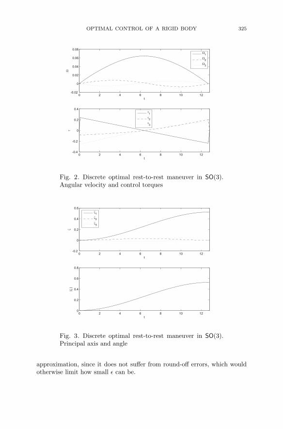
Fig. 2. Discrete optimal rest-to-rest maneuver in SO(3).Angular velocity and control torques
Fig. 3. Discrete optimal rest-to-rest maneuver in SO(3).Principal axis and angle
approximation, since it does not suffer from round-off errors, which wouldotherwise limit how small ε can be.

326 A. M. BLOCH, I. I. HUSSEIN, M. LEOK, and A. K. SANYAL
Fig. 4. Discrete optimal rest-to-rest maneuver in SO(3).Instantaneous rotation axis
In our numerical simulation, we computed an optimal trajectory for arest-to-rest maneuver, as illustrated in Figs. 2–4. Here, the maneuver timeis 12.8 sec, N = 128, and the moment of inertia is given by
J =
⎡
⎣13.25 −7.80 −11.40−7.80 16.25 4.71
−11.40 4.71 18.37
⎤
⎦ .
The prescribed maneuver corresponds to a rotation by π3 about the x-axis.
Since the moment of inertia tensor is not a multiple of the identity, andthe x-axis does not correspond to the axis of minimal inertia, the optimaltrajectory does not just involve a pure rotation about the x-axis. It is worthnoting that the results are not rotationally symmetric about the midpointof the simulation interval, which is due to the fact that our choice of up-date, Rk+1 = Rk exp(hΩk), does not exhibit time-reversal symmetry. In aforthcoming publication, we will introduce a reversible algorithm to addressthis issue. In particular, this will involve explicitly computing the station-arity conditions for the discrete optimal control problem constrained by thetime-symmetric Lie Stormer–Verlet method.
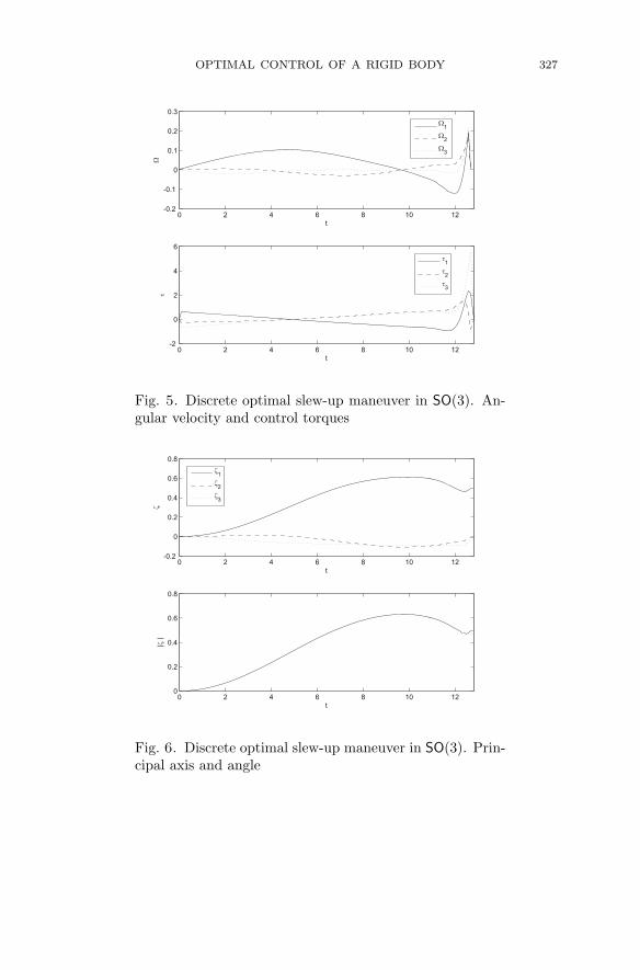
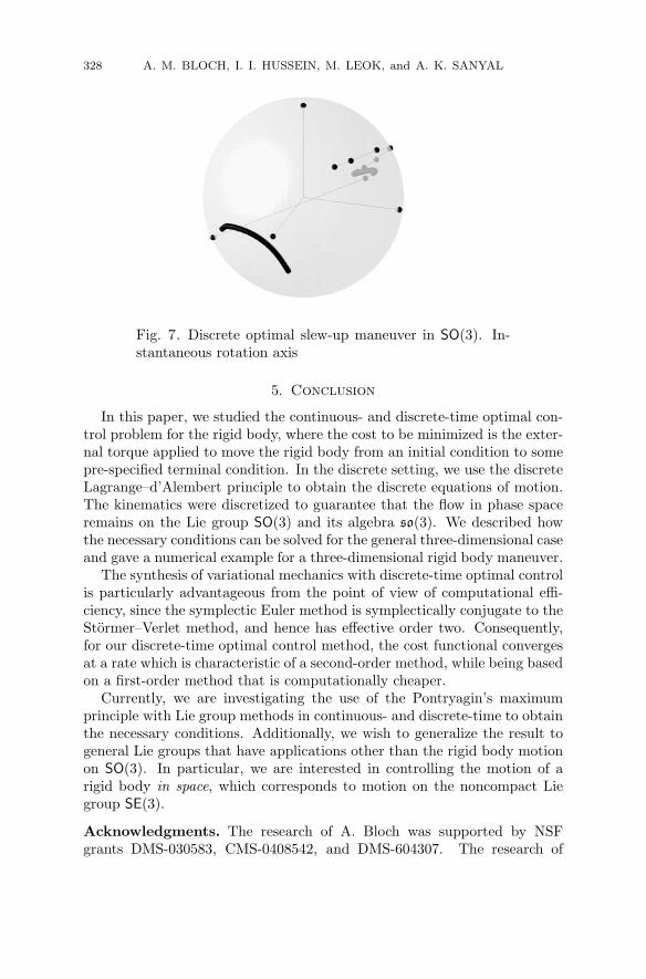
We also present results for an optimal slew-up maneuver, illustrated inFigs. 5–7. This uses the same moment of inertia tensor as in the previoussimulation, and the desired maneuver involves a rotation of π
6 about the
x-axis from rest to a final angular velocity of ΩN−1 =[0.3 0.2 0.3
]T,over a maneuver time of 12.8 sec, and N = 128.
OPTIMAL CONTROL OF A RIGID BODY 327
Fig. 5. Discrete optimal slew-up maneuver in SO(3). An-gular velocity and control torques
Fig. 6. Discrete optimal slew-up maneuver in SO(3). Prin-cipal axis and angle
328 A. M. BLOCH, I. I. HUSSEIN, M. LEOK, and A. K. SANYAL
Fig. 7. Discrete optimal slew-up maneuver in SO(3). In-stantaneous rotation axis
5. Conclusion
In this paper, we studied the continuous- and discrete-time optimal con-trol problem for the rigid body, where the cost to be minimized is the exter-nal torque applied to move the rigid body from an initial condition to somepre-specified terminal condition. In the discrete setting, we use the discreteLagrange–d’Alembert principle to obtain the discrete equations of motion.The kinematics were discretized to guarantee that the flow in phase spaceremains on the Lie group SO(3) and its algebra so(3). We described howthe necessary conditions can be solved for the general three-dimensional caseand gave a numerical example for a three-dimensional rigid body maneuver.
The synthesis of variational mechanics with discrete-time optimal controlis particularly advantageous from the point of view of computational effi-ciency, since the symplectic Euler method is symplectically conjugate to theStormer–Verlet method, and hence has effective order two. Consequently,for our discrete-time optimal control method, the cost functional convergesat a rate which is characteristic of a second-order method, while being basedon a first-order method that is computationally cheaper.
Currently, we are investigating the use of the Pontryagin’s maximumprinciple with Lie group methods in continuous- and discrete-time to obtainthe necessary conditions. Additionally, we wish to generalize the result togeneral Lie groups that have applications other than the rigid body motionon SO(3). In particular, we are interested in controlling the motion of arigid body in space, which corresponds to motion on the noncompact Liegroup SE(3).
Acknowledgments. The research of A. Bloch was supported by NSFgrants DMS-030583, CMS-0408542, and DMS-604307. The research of
OPTIMAL CONTROL OF A RIGID BODY 329
I. Hussein was supported by a WPI Faculty Development Grant. The re-search of M. Leok was partially supported by NSF grants DMS-0504747,DMS-0726263, and CAREER Award DMS-0747659. The research ofA. Sanyal was partially supported by a University of Hawaii Faculty Devel-opment Grant.
References
1. A. Agrachev, Yu. Sachkov, Control theory from the geometric view-point. Springer-Verlag, New York (2004).
2. J. Bonnans an J.Laurent-Varin, Computation of order conditions forsymplectic partitioned Runge–Kutta schemes with application to opti-mal control. Numer. Math. 103 (2006), 1–10.
3. E. Hairer, C. Lubich, and G. Wanner, Geometric numerical integration.Springer-Verlag, Berlin (2002).
4. , Geometric numerical integration illustrated by the Stormer—Verlet method. Acta Numer. 12 (2003), 399–450.
5. I. I. Hussein, D. J. Scheeres, and D. C. Hyland, Interferometric observa-tories in the Earth orbit. J. Guidance Control Dynam. 27 (2004), No. 2,297–301.
6. A. Iserles, H. Munthe-Kaas, S. P. Nørsett, A. Zanna, Lie group methods.Acta Numer. 9 (2000), 215–265.
7. O. Junge, J. E. Marsden, and S. Ober-Blobaum, Discrete mechanicsand optimal control. IFAC Congress, Praha (2005).
8. C. Kane, J. E. Marsden, M. Ortiz, and M. West, Variational integratorsand the newmark algorithm for conservative and dissipative mechanicalsystems. Int. J. Numer. Methods Engineering 49 (2000), No. 10, 1295–1325.
9. N. Khaneja, S. J. Glaser, and R. W. Brockett, Sub-Riemannian geome-try and optimal control of three spin systems. Phys. Rev. A 65 (2002),032301.
10. T. Lee, M. Leok, and N. McClamroch, Lie group variational integratorsfor the full body problem in orbital mechanics. Celest. Mech. Dynam.Astr. 98 (2007), No. 2, 121–144.
11. , Lie group variational integrators for the full body problem.Comput. Methods Appl. Mech. Eng. 196 (2007), Nos. 29–30, 2907–2924.
12. B. Leimkuhler and S. Reich, Simulating Hamiltonian dynamics. Cam-bridge Univ. Press, Cambridge (2004).
13. M. Leok, Generalized galerkin variational integrators. PreprintarXiv:math.NA/0508360 (2004).
14. T. Littell, R. Skeel, and M. Zhang, Error analysis of symplectic multipletime stepping. SIAM J. Numer. Anal. 34 (1997), No. 5, 1792–1807.
15. J. Lyness and C. Moler, Numerical differentiation of analytic functions.SIAM J. Numer. Anal. 4 (1967), 202–210.

330 A. M. BLOCH, I. I. HUSSEIN, M. LEOK, and A. K. SANYAL
16. J. Marsden and M. West, Discrete mechanics and variational integra-tors. Acta Numer. 10 (2001), 357–514.
17. J. E. Marsden and T. S. Ratiu, Introduction to mechanics and symme-try. Springer-Verlag, New York (1999).
18. J. Milnor, Morse theory. Princeton Univ. Press, Princeton (1963).19. J. P. Palao and R. Kosloff, Quantum computing by an optimal con-
trol algorithm for unitary transformations. Phys. Rev. Lett. 89 (2002),188301.
20. J. M. Sanz-Serna and M. P. Calvo, Numerical Hamiltonian problems.Chapman and Hall, London (1994)
21. H. Schaub, J. L. Junkins, and R. D. Robinett, New attitude penaltyfunctions for spacecraft optimal control problems. AIAA Guidance,Navigation, and Control Conference (1996).
22. D. Scheeres, E. Fahnestock, S. Ostro, J. Margot, L. Benner,S. Broschart, J. Bellerose, J. Giorgini, M. Nolan, C. Magri, P. Pravec,P. Scheirich, R. Rose, R. Jurgens, E. D. Jong, S. Suzuki, Dynamicalconfiguration of binary near-Earth asteroid (66391) 1999 KW4. Science314 (5803) (2006), 1280–1283.
23. S. L. Scrivener and R. C. Thompson, Survey of time-optimal attitudemaneuvers. J. Guidance Control Dynam. 17 (1994), No. 2, 225–233.
24. M. Suzuki, Improved Trotter-like formula. Phys. Lett. A 180 (1993),No. 3, 232–234.
(Received December 28 2007, received in revised form September 09 2008)
Authors’ addresses:A. M. BlochUniversity of MichiganE-mail: [email protected]
I. I. HusseinWorcester Polytechnic InstituteE-mail: [email protected]
M. LeokPurdue UniversityE-mail: [email protected]
A. K. SanyalUniversity of HawaiiE-mail: [email protected]