geometric sliding mode control: the linear and linearised ...andrew/notes/pdf/2002c.pdf ·...

Geometric sliding mode control:The linear and linearised theory∗

Ron M. Hirschorn† Andrew D. Lewis‡

2003/01/09

Last updated: 2006/09/28

Abstract

The idea of sliding mode control for stabilisation is investigated to determine itsgeometric features. A geometric definition is provided for a sliding submanifold, andfor various properties of a sliding submanifold. Sliding subspaces are considered forlinear systems, where a pole placement algorithm is given that complements existingalgorithms. Finally, it is shown that at an equilibrium for a nonlinear system with acontrollable linearisation, the sliding subspace for a linearisation gives rise to many localsliding submanifolds for the nonlinear system. This theory is exhibited on the standardpendulum/cart system.

Keywords. sliding mode control, linear systems, linearisation.

AMS Subject Classifications (2010). 93B12, 93B18, 93B27, 93B55.

1. Introduction

In sliding mode control, the idea is that one provides a surface on which the dynamicsof the system, when restricted to the surface, have desired properties, e.g., all trajectoriesasymptotically approach a desired equilibrium point. The surface should also have theproperty that one can, by a suitable control law, force trajectories to the surface in finitetime. In this way, one can ensure that the system eventually behaves as behaves the systemon the surface. Sometimes, in applications, the surface is obtained via the use of a linearisingoutput. A rather thorough review of the classical notion of sliding mode control is providedby Utkin [1992]. The topic is also covered in the book by Slotine and Li [1990], and a recentbook concerning sliding mode control is that of Edwards and Spurgeon [1998]. There isalso a significant number of journal papers devoted to sliding mode control, many of themconcerning specific applications of sliding mode control.

Our intent is to understand sliding mode control in a geometric way. In particular, wewish to place the emphasis on understanding the relationship between the surface and the

∗Preprint†Professor, Department of Mathematics and Statistics, Queen’s University, Kingston, ON K7L3N6, CanadaEmail: [email protected], URL: http://www.mast.queensu.ca/~ron/Research supported in part by a grant from the Natural Sciences and Engineering Research Council ofCanada.‡Professor, Department of Mathematics and Statistics, Queen’s University, Kingston, ON K7L3N6, CanadaEmail: [email protected], URL: http://www.mast.queensu.ca/~andrew/Research supported in part by a grant from the Natural Sciences and Engineering Research Council ofCanada.

1

2 R. M. Hirschorn and A. D. Lewis

ambient system dynamics, and, by exploiting this understanding, to develop some intuitionfor the design of sliding mode controllers. In this paper we consider this way of thinkingabout sliding mode control for linear systems, and for nonlinear systems near equilibriawith controllable linearisations. The emphasis of the present paper is not so much to givenew results, but to understand in a different light existing results concerning sliding modecontrol, and to better understand the very notion of sliding mode control. This insightfulmanner of presenting sliding mode control will be explored in subsequent papers where ourdifferent way of looking at things really does help to understand what one is doing.

In Section 2 we set up a general scheme for sliding mode control. We give generaldefinitions for various concepts related to sliding mode control. A key idea is the notionof a “restriction” of a system, which helps to clarify what is typically referred to as the“equivalent control.” We also present a simple example that illustrates our approach byproviding a simple, intuitive characterisation of all sliding mode controllers for the system.We investigate in detail the linear case in Section 3. Here we look for subspaces on whichthe dynamics can be specified to be stable. We provide a proof, different from that of Utkin[1992], that one can achieve any characteristic polynomial on the sliding subspace. As acorollary to our proof we provide a characterisation of all the ways in which one can obtaina sliding subspace with a certain characteristic polynomial. For linear systems we alsoprovide algorithms, defined in a geometrically intuitive manner, that steer the system to agiven sliding subspace in finite time. Although there are many ways to do this, we considertwo, one being local in nature and using bounded controls, and the other being global, butperhaps requiring unbounded controls. In Section 5 we consider nonlinear systems at anequilibrium with a controllable linearisation. We show that for these systems the linearsliding subspace defines a many local sliding submanifolds for the nonlinear system. Forthe pendulum/cart system, we compare the performance of a sliding mode controller witha LQR controller.

There is, of course, a wealth of papers which use sliding mode control, as it is often quiteeffective in applications. The intent in this paper is to propose a way of thinking aboutsliding mode control, and to illustrate that this way of thinking about sliding mode controloffers some nice insights into existing strategies. In future work we will explore how to useour geometric approach in cases that are more interesting than those that are linear, orhave controllable linearisations. Since the preponderance of existing applications of slidingmode control employ some sort of linear controllability assumption, this future work willwell exhibit the utility of a geometric approach such as is initiated in this paper.

2. A general picture of sliding mode control

In this section we develop our geometric approach to sliding mode control. We intendto develop a sufficiently general picture to allow for applications more general than areconsidered in this paper.

2.1. Setup. In this paper, for concreteness and to emphasise the geometric nature of ourconstructions, we consider control-affine systems. By a control-affine system we mean atriple Σ = (M,F = {f0, f1, . . . , fm}, U) where M is a smooth manifold of dimension n, Fis a collection of smooth vector fields on M , and U ⊂ Rm is the set within which controlswill take their values. Thus a controlled trajectory is a pair (ξ : I → M,u : I → U) of

Geometric sliding mode control: The linear and linearised theory 3

curves defined on the interval I ⊂ R with u measurable and which together satisfy thedifferential equation

ξ(t) = f0(ξ(t)) +m∑a=1

ua(t)fa(ξ(t)).

Throughout the paper we make the assumption that the distribution F whose fibre at x ∈Mis defined by

Fx = spanR(f1(x), . . . , fm(x))

has constant rank. We do not wish that considerations of the exact nature of the controlset get in the way of our geometric constructions, so we ask that U = Rm, unless we stateotherwise. In practice, of course, one typically has only finite control action available. Wewill consider the consequences of this at various times, but to simplify parts of the generalpresentation we will take as default the case where control values are unrestricted. If X ⊂Mis an open submanifold then Σ|X denotes the control-affine system (X,F|X, U), where F|Xis the collection of vector fields in F, restricted to X.

2.2. Restrictions of control-affine systems. We wish to have our sliding submanifold havethe property that we may restrict the system to it. In cases when the restricted systemis unique, the control giving rise to this restriction is called the “equivalent control.” Inthis section, we formulate this idea of restriction to a submanifold, and of characterising theequivalent control, in a slightly different manner than is the norm. We consider control-affinesystems Σ = (M,F = {f0, f1, . . . , fm}, U = Rm) and Σ = (S, F = {f0, f1, . . . , fm}, U =Rm) with the property that S is a submanifold of M . We shall say that Σ is a restrictionof Σ if for every controlled trajectory (ξ, u) for Σ there is a control u for which (iS ◦ ξ, u) is acontrolled trajectory for Σ, where iS : S →M is the inclusion. A submanifold S is Σ-rigidif

1. there is only one control-affine system Σ = (S, F, U = Rm) that is a restriction of Σand if

2. F = {f0} for some smooth vector field f0 on S.

The following result characterises Σ-rigid submanifolds.

2.1 Proposition: For a control-affine system Σ = (M,F, U = Rm) a submanifold S ⊂ Mis Σ-rigid if for each x ∈ S we have TxM = TxS ⊕ Fx. Conversely, if S is Σ-rigid thenTxS ∩ Fx = {0}.

Proof: First suppose that TxM = TxS ⊕ Fx for each x ∈ S and let (ξ, u) be a controlledtrajectory for Σ passing through x at time, say, t ∈ R, and having the property thatξ(I) ⊂ S. Then

ξ(t) = f0(x) +

m∑a=1

ua(t)fa(x) ∈ TxS.

This means

f0(x) +m∑a=1

ua(t)fa(x)


lies in the subspace TxS ⊂ TxM as well as lying in the affine subspace

f0(x) + Fx ={f0(x) +

m∑a=1

uafa(x)∣∣∣ u ∈ Rm

}.

We claim that since TxM = TxS⊕Fx we have (f0(x)+Fx)∩TxS = {vx} for some vx ∈ TxM .Indeed, let {v1, . . . , vk} be a basis for TxS and let {vk+1, . . . , vn} be a basis for Fx. Theequation

c1v1 + · · ·+ ckvk + ck+1vk+1 + · · ·+ cnvn = f0(x)

then has a unique solution for the constants c1, . . . , cn. We also have

TxS 3 c1v1 + · · ·+ ckvk = f0(x)− ck+1vk+1 − · · · − cnvn ∈ f0(x) + Fx,

so it follows that (f0(x) + Fx) ∩ TxS 6= ∅. To show that the intersection consists of asingle vector also follows from elementary linear algebra. This shows that TxM = TxS⊕Fximplies that (f0(x) + Fx) ∩ TxS = {vx} for some vx ∈ TxM , thus showing that there is aunique vector f1(x) ∈ Fx for which f0(x)+f1(x) ∈ TxS. Thus S is indeed Σ-rigid by takingF = {f0 + f1}, thinking of f0 + f1 as being a vector field on S.

Conversely, suppose that S is Σ-rigid. Then for each x ∈ S there exists a uniquef1(x) ∈ Fx with the property that f0(x)+f1(x) ∈ TxS. Let us abbreviate vx = f0(x)+f1(x).Thinking of f0(x) + Fx and TxS as submanifolds of TxM this means that Tvx(f0(x) + Fx)and Tvx(TxS) intersect in {0}. However, since Tvx(f0(x) + Fx) ' Fx and Tvx(TxS) ' TxSthis part of the proposition follows. �

In the case that TxM = TxS ⊕ Fx, let prS : TM |S → TS be the projection onto thetangent bundle of S and let prF : TM |S → F|S be the projection onto the input distributionon S, both defined with respect to the decomposition TxM = TxS ⊕ Fx.

2.2 Remark: In most of the literature on sliding mode control, sliding surfaces are assumedto be rigid. The equivalent control is then often characterised by considering the limits ofclosed-loop controls off the sliding surface as they approach the sliding surface. It is notperfectly obvious that the equivalent control defined in this way is unique, i.e., does notdepend on the control off the surface. The characterisation of Proposition 2.1 makes thisclear. Indeed, the equivalent control uS : S → Rm is defined as satisfying

prF

(f0(x) +

m∑a=1

uaS(x)fa(x))

= 0, x ∈ S.

Note that for the equivalent control to really be unique, the vector fields {f1, . . . , fm} shouldbe linearly independent. If this is not true, then one should really say that the vector field∑m

a=1 uaSfa is unique, even though the coefficients uaS , a ∈ {1, . . . ,m}, are not. In either

case, the important thing is that the dynamics on S are simply prescribed by the vectorfield f0 that is defined by

f0(x) = prS(f0(x)), x ∈ S. •

2.3. Sliding submanifolds and their properties. In this section we provide a general char-acterisation of sliding submanifolds and some of the properties they may possess. If S ⊂M ,iS : S →M denotes the inclusion.


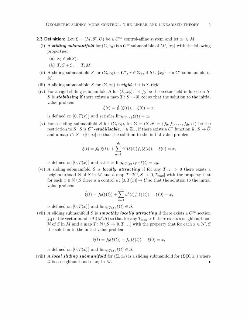
2.3 Definition: Let Σ = (M,F, U) be a C∞ control-affine system and let x0 ∈M .

(i) A sliding submanifold for (Σ, x0) is a C∞ submanifold ofM\{x0} with the followingproperties:

(a) x0 ∈ cl(S);

(b) TxS + Fx = TxM .

(ii) A sliding submanifold S for (Σ, x0) is Cr, r ∈ Z+, if S ∪ {x0} is a Cr submanifold ofM .

(iii) A sliding submanifold S for (Σ, x0) is rigid if it is Σ-rigid.

(iv) For a rigid sliding submanifold S for (Σ, x0), let f0 be the vector field induced on S.S is stabilising if there exists a map T : S → ]0,∞] so that the solution to the initialvalue problem

ξ(t) = f0(ξ(t)), ξ(0) = x,

is defined on [0, T (x)[ and satisfies limt↑T (x) ξ(t) = x0.

(v) For a sliding submanifold S for (Σ, x0), let Σ = (S, F = {f0, f1, . . . , fm, U) be therestriction to S. S is Cr-stabilisable , r ∈ Z+, if there exists a Cr function u : S → Uand a map T : S → ]0,∞] so that the solution to the initial value problem

ξ(t) = f0(ξ(t)) +

m∑a=1

ua(ξ(t))fa(ξ(t)), ξ(0) = x,

is defined on [0, T (x)[ and satisfies limt↑T (x) iS ◦ ξ(t) = x0.

(vi) A sliding submanifold S is locally attracting if for any Tmax > 0 there exists aneighbourhood N of S in M and a map T : N \ S → ]0, Tmax] with the property thatfor each x ∈ N\S there is a control u : [0, T (x)[→ U so that the solution to the initialvalue problem

ξ(t) = f0(ξ(t)) +m∑a=1

ua(t)fa(ξ(t)), ξ(0) = x,

is defined on [0, T (x)[ and limt↑T (x) ξ(t) ∈ S.

(vii) A sliding submanifold S is smoothly locally attracting if there exists a C∞ sectionfcl of the vector bundle F|(M\S) so that for any Tmax > 0 there exists a neighbourhoodN of S in M and a map T : N\S → ]0, Tmax] with the property that for each x ∈ N\Sthe solution to the initial value problem

ξ(t) = f0(ξ(t)) + fcl(ξ(t)), ξ(0) = x,

is defined on [0, T (x)[ and limt↑T (x) ξ(t) ∈ S.

(viii) A local sliding submanifold for (Σ, x0) is a sliding submanifold for (Σ|X, x0) whereX is a neighbourhood of x0 in M . •


2.4 Remark: 1. We exclude x0 from being in S in order to allow certain examples whereit is helpful to be able to design S to have a singularity at x0.

2. In part (v) of the definition, one can allow other forms of stabilisability of the restric-tion to S, if desired. •

2.4. A nonlinear controller for a simple linear system. To give an indication of how onemay use the geometric approach, we consider a rather simple example,

x1 = x2

x2 = u,(2.1)

and we see what it might mean to design a “sliding mode controller” for the system thatstabilises x0 = (0, 0). In terms of the definitions of the preceding section, we shall design arigid stabilising smoothly locally attracting sliding submanifold S. Let us write (2.1) as asingle-input control affine system Σ = (R2,F = {f0, f1}, U) where

f0(x1, x2) = x2∂

∂x1, f1(x1, x2) =

∂

∂x2.

We first choose S so that it contains x0 in its closure. Next we must choose S so that thesystem (2.1) restricts to it. By Proposition 2.1 this means that we should choose S so that,away from x0, TxS is not parallel to the vector (0, 1). Another requirement of S is that thedynamics, when restricted to S as in Proposition 2.1, should have x0 as an asymptoticallystable “equilibrium point.” The geometry underlying this second condition is more subtleto understand, but can still be done in an intuitive manner by considering the vector fieldf0, and how it influences the restriction to S. In Figure 1 we show how this produces a

S

f0(x)

TxS

x ∈ S

f(x)

S

f0(x)

TxS

x ∈ Sf(x)

Figure 1. The character of the restricted dynamics in the (−,+)-quadrant (left) and in the (+,+)-quadrant (right)

vector field f0 on S for x2 > 0. We see that when x1 > 0 the restricted dynamics on Srenders x0 unstable, whereas the behaviour on S is desirable for x1 < 0. Thus we are forcedto ask that S intersect the upper half plane only in the (−,+)-quadrant. Similar argumentsdemand that S intersect the lower half place in the (+,−)-quadrant.

At this point we have a pretty good idea of what a stabilising rigid sliding surfacemay look like. It must be the graph of a strictly decreasing function that passes throughx0 = (0, 0). The only remaining issue to confront is how it should pass through x0. It may


easily be checked that as long as S does not have a vertical tangency at x0, the dynamicson S, and the control giving rise to these dynamics, is well behaved. However, verticaltangencies are also allowed for S at x0, provided that they are not “too vertical.” We shallnot address this in the present paper, although it will be investigated in a future paper.

Now that we have a sliding surface on which the dynamics behave in a satisfactorymanner we should set about forcing the system trajectories near S to reach the slidingsurface in finite time. In fact, in this example one can easily design bounded controls thatsteer the system to S in finite time, although this time will not be uniformly bounded. InFigure 2 we show the closed-loop phase portrait for the system having chosen

-1.5 -1 -0.5 0 0.5 1 1.5 2

-1.5

-1

-0.5

0

0.5

1

1.5

2

x1

x2

Figure 2. Phase portrait for closed-loop controller with a slidingsurface S = {(x1,−x1) | x1 ∈ R}

S = {(x1, x2) ∈ R2 \ {(0, 0)} | x1 = 12x

22},

and having chosen a constant control (of magnitude 5 in this case) away from S to steer to S.Note that S is a C1 rigid, stabilising submanifold. An interesting feature of this particularsliding submanifold is that the control required to stay on S has constant magnitude 1.Thus the closed-loop phase portrait of Figure 2 is obtained with controls taking values inthe set {−5,−1, 1, 5}.

3. Geometric sliding mode control for linear systems

The ideas so far have been general in character. In this section we consider the particularcase of linear systems and rigid sliding subspaces. The results in this case are known, of


course [e.g., Utkin 1992, §7.2]. However, our approach is slightly different. This leads to,for example, a complete characterisation in Proposition 3.2 of rigid sliding subspaces andhow to obtain them.

We let U and V be R-vector spaces of dimension m and n, and say that a linear systemon V with inputs in U is a pair Λ = (A,B) with A ∈ L(V;V) and B ∈ L(U;V). Note thata linear system is also a control-affine system, so all the definitions of Section 2 apply. Asusual the equations governing the linear system Λ are

ξ(t) = A(ξ(t)) +B(u(t)). (3.1)

We will assume without loss of generality that B is injective. (If it is not, let U = U/ ker(B)and B(u+ ker(B)) = B(u). Then (A, B) is a linear system on V with inputs in U , and B isinjective. Furthermore, if (ξ, u) is a controlled trajectory for (A,B) then (ξ, u+ ker(B)) isa controlled trajectory for (A, B).) A sliding submanifold for (Λ, 0) that is also a subspaceis a sliding subspace .

Our objective in this section is to consider a systematic method for producing slidingsubspaces on which the dynamics have a prescribed characteristic polynomial. This is donein Section 3.1. In Section 3.2 we consider the problem of steering the system to the slidingsubspace in a systematic way. In doing so, we provide a geometric characterisation of thestandard output-based sliding mode control law. Our characterisation does not rely on thepresence of an output (typically denoted “s” in the sliding mode control literature).

3.1. Sliding subspaces for linear systems. If S is a rigid sliding subspace for Λ = (A,B)then we must have V = S ⊕ image(B). Denote prB : V → image(B) and prS : V → S theprojections relative to the direct sum decomposition in this case. The inclusions we denoteiB : image(B) → V and iS : S → V. The vector field on S obtained by restriction of thesystem (3.1) will be obtained by projecting A(x) to S for x ∈ S. The control at x ∈ S willthen be the unique (since B is assumed injective) u ∈ U satisfying B(u) = −prB(A(x)).

The following result provides the essential feature of the preceding constructions. If L ∈L(V;V) then spec(L) ⊂ C denotes the eigenvalues of L and if P ∈ R[λ] then spec(P ) ⊂ Cdenotes the roots of P .

3.1 Theorem: Let V and U be R-vector spaces of dimension n and m, respectively, and letA ∈ L(V;V) and B ∈ L(U;V) be linear maps with the property that (A,B) is controllable.If P ∈ R[λ] is a monic polynomial of degree n−m then there exists a subspace S with thefollowing properties:

(i) V = image(B)⊕ S;

(ii) spec(AS) = spec(P ) where AS = prS ◦A ◦ iS.

Proof: Let us choose a linear map F0 ∈ L(V;U) for which there exists bases {v1, . . . , vn} forV and {u1, . . . , um} for U having the property that the representations of A+B ◦F0 and Bin these bases are in Brunovsky form. Thus, letting the matrix representation of A+B ◦F0

be denoted A ∈ Rn×n and the matrix representation of B be denoted B ∈ Rn×m we have

A =

Jκ1 0 · · · 00 Jκ2 · · · 0...

.... . .

...0 0 · · · Jκm

, B =

eκ1 0 · · · 00 eκ2 · · · 0...

.... . .

...0 0 · · · eκm

,


where

Jκj =

0 1 0 · · · 0 00 0 1 · · · 0 0...

......

. . ....

...0 0 0 · · · 0 10 0 0 · · · 0 0

︸︷︷︸

κj

κj , eκj =

00...01

κj , j ∈ {1, . . . ,m},

and where κ = (κ1, . . . , κm) are the controllability indices. Now consider an arbitraryF ∈ Rm×n and write it as

F =

f11 f12 · · · f1m

f21 f22 · · · f2m...

.... . .

...fm1 fm2 · · · fmm,

for f jk ∈ R1×κk , j, k ∈ {1, . . . ,m}. Let us write f jk as

f jk =[fjk1 fjk2 · · · fjkκk

].

We shall decompose Rm×n as R(m−1)×n ⊕ R1×n by writing F ∈ Rm×n as

F =

f1...

fm−1

0

+

0...0fm

, (3.2)

where f j ∈ R1×n, j ∈ {1, . . . ,m}. We denote by π1(F ) the first term on the right-handside of the above equation, and by π2(F ) the second term.

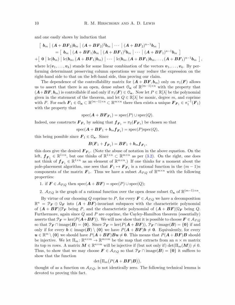
We now consider the single input bm = (0, . . . , 0, 1). We claim that the determinant ofthe controllability matrix for the single-input system (A+BF , bm) depends only on π1(F ).That is to say, if F 1,F 2 ∈ Rm×n have the property that π1(F 1 − F 2) = 0, then

det[bm (A+BF 1)bm · · · (A+BF 1)n−1bm

]= det

[bm (A+BF 2)bm · · · (A+BF 2)n−1bm

].

Indeed, if π1(F 1 − F 2) = 0 then there exists f ∈ R1×n so that

F 2 = F 1 +

0...0f

.In this case we have

BF 2 = BF 1 + bmf ,


and one easily shows by induction that[bm (A+BF 2)bm (A+BF 2)2bm · · · (A+BF 2)n−1bm

]=[bm (A+BF 1)bm (A+BF 1)2bm · · · (A+BF 1)n−1bm

]+[

0 lc(bm) lc(bm, (A+BF 1)bm) · · · lc(bm, (A+BF 1)bm, . . . , (A+BF 1)n−1bm],

where lc(v1, . . . ,vk) stands for some linear combination of the vectors v1, . . . ,vk. By per-forming determinant preserving column operations we may reduce the expression on theright-hand side to that on the left-hand side, thus proving our claim.

The dependence of the controllability matrix for (A +BF , bm) only on π1(F ) allowsus to assert that there is an open, dense subset Oκ of R(m−1)×n with the property that(A+BF , bm) is controllable if and only if π1(F ) ∈ Oκ. Now let P ∈ R[λ] be the polynomialgiven in the statement of the theorem, and let Q ∈ R[λ] be monic, degree m, and coprimewith P . For each F 1 ∈ Oκ ⊂ R(m−1)×n ⊂ Rm×n there then exists a unique F F 1 ∈ π−1

1 (F 1)with the property that

spec(A+BF F 1) = spec(P ) ∪ spec(Q).

Indeed, one constructs F F 1 by asking that fF 1= π2(F F 1) be chosen so that

spec(A+BF 1 + bmfF 1) = spec(P )spec(Q),

this being possible since F 1 ∈ Oκ. Since

B(F 1 + fF 1) = BF 1 + bmfF 1

,

this does give the desired F F 1 . (Note the abuse of notation in the above equation. On theleft, fF 1

∈ R1×n, but one thinks of R1×n ⊂ Rm×n as per (3.2). On the right, one doesnot think of fF 1

∈ R1×n as an element of Rm×n.) If one thinks for a moment about thepole-placement algorithm, one sees that F 1 7→ F F 1 is a rational function in the (m − 1)ncomponents of the matrix F 1. Thus we have a subset AP,Q of Rm×n with the followingproperties:

1. if F ∈ AP,Q then spec(A+BF ) = spec(P ) ∪ spec(Q);

2. AP,Q is the graph of a rational function over the open dense subset Oκ of R(m−1)×n.

By virtue of our choosing Q coprime to P , for every F ∈ AP,Q we have a decompositionRn = PF ⊕ QF into (A + BF )-invariant subspaces with the characteristic polynomialof (A + BF )|PF being P , and the characteristic polynomial of (A + BF )|QF being Q.Furthermore, again since Q and P are coprime, the Cayley-Hamilton theorem (essentially)asserts that PF = ker(P (A+BF )). We will now show that it is possible to choose F ∈ AP,Q

so that PF ∩ image(B) = {0}. Since PF = ker(P (A+BF )), PF ∩ image(B) = {0} if andonly if for every b ∈ image(B) \ {0} we have P (A + BF )b 6= 0. Equivalently, for everyu ∈ Rm \ {0} we should have P (A+BF )Bu 6= 0. This means that P (A+BF )B shouldbe injective. We let Πm : Rn×m → Rm×m be the map that extracts from an n×m matrixits top m rows. A matrix M ∈ Rn×m will be injective if (but not only if) det(Πm(M)) 6= 0.Thus, to show that we may choose F ∈ AP,Q so that PF ∩ image(B) = {0} it suffices toshow that the function

det(Πm

(P (A+BF )B

)),

thought of as a function on AP,Q, is not identically zero. The following technical lemma isdevoted to proving this fact.


1 Lemma: There exists a curve α 7→ F α in AP,Q with the property that

α 7→ det(Πm

(P (A+BF α)B

))is a nontrivial polynomial in α.

Proof: We take

F α =

0 · · · α 1 · · · 0 0 · · · 0 0 · · · 00 · · · 0 0 · · · α 1 · · · 0 0 · · · 0...

. . ....

.... . .

......

. . ....

.... . .

...0 · · · 0 0 · · · 0 0 · · · α 1 · · · 0f1 · · · fρ1 fρ1+1 · · · fρ2 fρ2+1 · · · fρm−1 fρm−1+1 · · · fρm

where ρj =

∑ji=1 κi, and where the last row of F α is chosen so that Aα , A +BF α has

characteristic polynomial P (λ)Q(λ).For i ∈ {1, . . . ,m} define integers `i by

`1 = κm − 1, `2 = `1 + κm−1 − 1, . . . , `m = `m−1 + κ1 − 1.

For k ∈ {0, 1, . . . , n−m} define integers ri(k), i ∈ {1, . . . ,m}, as follows. For k = 0 we let

ri(0) =i∑

j=1

κj , i ∈ {1, . . . ,m}.

For k ∈ {1, . . . , `1} we let

ri(k) = κ1 + · · ·+ κi, i ∈ {1, . . . ,m− 1}rm(k) = n− k.

Generally, for k ∈ {`j + 1, . . . , `j+1} define

ri(k) = κ1 + · · ·+ κi, i ∈ {1, . . . ,m− j − 1}rm−j(k) = n− k − j

...

rm(k) = n− k.

IfP (λ) = λn−m + pn−m−1λ

n−m−1 + · · ·+ p1λ+ p0,

for k ∈ {0, 1, . . . , n−m} we denote by Pk the polynomial

Pk(λ) = λk + pn−1λk−1 + · · ·+ pn−kλ+ pn−k−1.

With this notation, we let Mα(k), k ∈ {0, 1, . . . , n − m}, be the m × m matrix whoseith row is the ri(k)th row of Pk(Aα)B. Since ri(n − m) = i, i ∈ {1, . . . ,m}, Mα(n −m) = Πm(P (Aα)B). A messy iterative computation shows that det(Mα(k)) is a monicpolynomial in α of degree `1 + · · ·+ `j if k ∈ {`j , . . . , `j+1}. In particular, this calculationshows that det

(Πm(P (Aα)B)

)is a monic polynomial of degree `1 + · · ·+ `m, and from this

the lemma follows. H


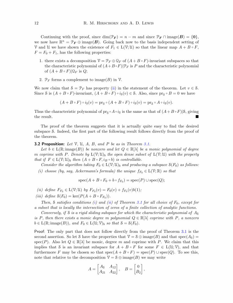
Continuing with the proof, since dim(PF ) = n −m and since PF ∩ image(B) = {0},we now have Rn = PF ⊕ image(B). Going back now to the basis independent setting ofV and U we have shown the existence of F1 ∈ L(V;U) so that the linear map A + B ◦ F ,F = F0 + F1, has the following properties:

1. there exists a decomposition V = PF ⊕QF of (A+B ◦F )-invariant subspaces so thatthe characteristic polynomial of (A+B ◦F )|PF is P and the characteristic polynomialof (A+B ◦ F )|QF is Q;

2. PF forms a complement to image(B) in V.

We now claim that S = PF has property (ii) in the statement of the theorem. Let v ∈ S.Since S is (A+B ◦ F )-invariant, (A+B ◦ F ) ◦ iS(v) ∈ S. Also, since prS ◦B = 0 we have

(A+B ◦ F ) ◦ iS(v) = prS ◦ (A+B ◦ F ) ◦ iS(v) = prS ◦A ◦ iS(v).

Thus the characteristic polynomial of prS ◦A ◦ iS is the same as that of (A+B ◦F )|S, givingthe result. �

The proof of the theorem suggests that it is actually quite easy to find the desiredsubspace S. Indeed, the first part of the following result follows directly from the proof ofthe theorem.

3.2 Proposition: Let V, U, A, B, and P be as in Theorem 3.1.Let b ∈ L(R; image(B)) be nonzero and let Q ∈ R[λ] be a monic polynomial of degree

m coprime with P . Denote by L(V;U)b the open dense subset of L(V;U) with the propertythat if F ∈ L(V;U)b then (A+B ◦ F, iB ◦ b) is controllable.

Consider the algorithm taking F0 ∈ L(V;U)b and producing a subspace S(F0) as follows:

(i) choose (by, say, Ackermann’s formula) the unique fF0 ∈ L(V;R) so that

spec(A+B ◦ F0 + b ◦ fF0) = spec(P ) ∪ spec(Q);

(ii) define FF0 ∈ L(V;U) by FF0(v) = F0(v) + fF0(v)b(1);

(iii) define S(F0) = ker(P (A+B ◦ FF0)).

Then, S satisfies conditions (i) and (ii) of Theorem 3.1 for all choice of F0, except fora subset that is locally the intersection of zeros of a finite collection of analytic functions.

Conversely, if S is a rigid sliding subspace for which the characteristic polynomial of AS

is P , then there exists a monic degree m polynomial Q ∈ R[λ] coprime with P , a nonzerob ∈ L(R; image(B)), and F0 ∈ L(U;V)b so that S = S(F0).

Proof: The only part that does not follow directly from the proof of Theorem 3.1 is thesecond assertion. So let S have the properties that V = S⊕ image(B) and that spec(AS) =spec(P ). Also let Q ∈ R[λ] be monic, degree m and coprime with P . We claim that thisimplies that S is an invariant subspace for A + B ◦ F for some F ∈ L(U;V), and thatfurthermore F may be chosen so that spec(A + B ◦ F ) = spec(P ) ∪ spec(Q). To see this,note that relative to the decomposition V = S⊕ image(B) we may write

A =

[AS A12

A21 A22

], B =

[0B2

],


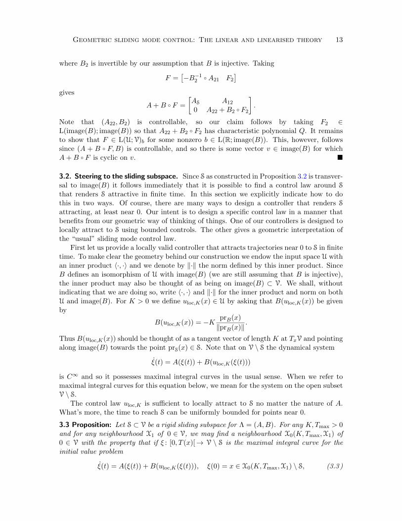
where B2 is invertible by our assumption that B is injective. Taking

F =[−B−1

2◦A21 F2

]gives

A+B ◦ F =

[AS A12

0 A22 +B2 ◦ F2

].

Note that (A22, B2) is controllable, so our claim follows by taking F2 ∈L(image(B); image(B)) so that A22 + B2 ◦ F2 has characteristic polynomial Q. It remainsto show that F ∈ L(U;V)b for some nonzero b ∈ L(R; image(B)). This, however, followssince (A + B ◦ F,B) is controllable, and so there is some vector v ∈ image(B) for whichA+B ◦ F is cyclic on v. �

3.2. Steering to the sliding subspace. Since S as constructed in Proposition 3.2 is transver-sal to image(B) it follows immediately that it is possible to find a control law around S

that renders S attractive in finite time. In this section we explicitly indicate how to dothis in two ways. Of course, there are many ways to design a controller that renders S

attracting, at least near 0. Our intent is to design a specific control law in a manner thatbenefits from our geometric way of thinking of things. One of our controllers is designed tolocally attract to S using bounded controls. The other gives a geometric interpretation ofthe “usual” sliding mode control law.

First let us provide a locally valid controller that attracts trajectories near 0 to S in finitetime. To make clear the geometry behind our construction we endow the input space U withan inner product 〈·, ·〉 and we denote by ‖·‖ the norm defined by this inner product. SinceB defines an isomorphism of U with image(B) (we are still assuming that B is injective),the inner product may also be thought of as being on image(B) ⊂ V. We shall, withoutindicating that we are doing so, write 〈·, ·〉 and ‖·‖ for the inner product and norm on bothU and image(B). For K > 0 we define uloc,K(x) ∈ U by asking that B(uloc,K(x)) be givenby

B(uloc,K(x)) = −K prB(x)

‖prB(x)‖.

Thus B(uloc,K(x)) should be thought of as a tangent vector of length K at TxV and pointingalong image(B) towards the point prS(x) ∈ S. Note that on V \ S the dynamical system

ξ(t) = A(ξ(t)) +B(uloc,K(ξ(t)))

is C∞ and so it possesses maximal integral curves in the usual sense. When we refer tomaximal integral curves for this equation below, we mean for the system on the open subsetV \ S.

The control law uloc,K is sufficient to locally attract to S no matter the nature of A.What’s more, the time to reach S can be uniformly bounded for points near 0.

3.3 Proposition: Let S ⊂ V be a rigid sliding subspace for Λ = (A,B). For any K,Tmax > 0and for any neighbourhood X1 of 0 ∈ V, we may find a neighbourhood X0(K,Tmax,X1) of0 ∈ V with the property that if ξ : [0, T (x)[→ V \ S is the maximal integral curve for theinitial value problem

ξ(t) = A(ξ(t)) +B(uloc,K(ξ(t))), ξ(0) = x ∈ X0(K,Tmax,X1) \ S, (3.3 )


then

(i) T (x) ≤ Tmax,

(ii) ξ(t) ∈ X1 for t ∈ [0, T (x)[ , and

(iii) limt↑T (x) ξ(t) ∈ S.

Proof: For the proof let us extend the inner product 〈·, ·〉 on image(B) to all of V, and doso in such a way that S is orthogonal to image(B). The extended inner product and normwe still denote by 〈·, ·〉 and ‖·‖, respectively. The induced norm on L(V;V) we denote by||| · |||. Denote by BR(x) the open ball of radius R centred at x.

Let us first obtain an estimate on the growth of ξ(t). We let ψ(x) = 12‖x‖

2 and compute

dψ

dt(ξ(t)) = 〈A(ξ(t)), ξ(t)〉 − K

‖prB(ξ(t))‖〈prB(ξ(t)), ξ(t)〉

= 〈A(ξ(t)), ξ(t)〉 −K‖prB(ξ(t))‖≤ |||A|||‖ξ(t)‖2 = 2|||A|||ψ(ξ(t)),

where we have used the Cauchy-Bunyakovsky-Schwarz inequality. By Gronwall’s lemma itnow follows that

ψ(t) ≤ ψ(0)e2|||A|||t

=⇒ ‖ξ(t)‖ ≤ ‖ξ(0)‖e|||A|||t. (3.4)

Now let us obtain an estimate governing the behaviour of the distance of ξ(t) from S.Define φ : V→ R by φ(x) = 1

2‖prB(x)‖2. We then have

dφ

dt(ξ(t)) =

⟨prB ◦A(ξ(t))),prB(ξ(t))

⟩−K‖prB(ξ(t))‖

≤ ‖prB ◦A(ξ(t))‖‖prB(ξ(t))‖ −K‖prB(ξ(t))‖

≤(|||prB ◦A|||‖ξ(t)‖ −K

)√φ(ξ(t))

≤(|||prB ◦A|||‖ξ(0)‖e|||A|||t −K

)√φ(ξ(t)),

where we have used the Cauchy-Bunyakovsky-Schwarz inequality along with (3.4). ApplyingGronwall’s lemma to the last inequality gives

φ(ξ(t)) ≤(C1‖ξ(0)‖(eC2t − 1) + C2(2

√φ(ξ(0))−Kt)

)24C2

2

≤(C1‖ξ(0)‖(eC2t − 1) + C2(

√2‖ξ(0)‖ −Kt)

)24C2

2

,

whereC1 = |||prB ◦A|||, C2 = |||A|||.

We define fα : R→ R by

fα(t) = C1α(eC2t − 1) + C2(√

2α−Kt),


We now show that for fixed positive constants C1 and C2, for any ε > 0 it is possible tochoose α so that fα has a root in [0, ε[ . To show this note that for t ∈ [0, ε] we have

fα(t) ≤ fα,ε(t) , C1α(eC2ε − 1) + C2(√

2α−Kt).

Thus it suffices to show that we may choose α sufficiently small that fα,ε has a root in [0, ε[ .This, however, is clear. Indeed, fα,ε is a linear function of t satisfying

fα,ε(0) = α(C1(eC2ε − 1) +

√2C2

), f ′α,ε(0) = −KC2.

By choosing α sufficiently small, fα,ε can be made to have a positive root as small as onelikes.

To complete the proof, let R1 > 0 have the property that BReC2Tmax (0) ⊂ X1 and letR2 > 0 have the property that fR2 has a root in ]0, Tmax[ . Define R = min{R1, R2}. TakingX0(K,Tmax,X1) = BR(0) gives the result. �

3.4 Remark: If A is Hurwitz, then the condition that the time to reach S be uniformlybounded can be relaxed (i.e., take Tmax =∞) with the ensuing advantage of being able totake X0(Tmax) = V. On the other hand if one demands at least of the following propertiesof the control law:

(i) the time to reach S be bounded uniformly in x by Tmax;

(ii) A be allowed to be non-Hurwitz;

then X0(Tmax) will have to be contained in a compact subset containing 0. •Now let us define a global control law, again in a geometric manner. For x ∈ V \ S we

define uglob,K(x) ∈ U by

B(uglob,K(x)) = uloc,K(x)− prB ◦A(x).

The idea here is simply that we augment our local control law with a “cancellation of asmuch of the uncontrolled dynamics as possible.” Such interpretations aside, let us showthat this control law does in fact globally attract trajectories to S.

3.5 Proposition: Let S ⊂ V be a rigid sliding subspace for Λ = (A,B). For each x ∈ V \ Sthere exists T (x) > 0 so that the maximal integral curve for the initial value problem

ξ(t) = A(ξ(t)) +B(uglob,K(ξ(t))), ξ(0) = x

is defined on [0, T (x)[ and so that limt↑T (x) ξ(t) ∈ S.

Proof: As in the proof of Proposition 3.3, we extend the inner product on image(B) to allof V so that S is orthogonal to image(B), and we adopt the notation introduced in thatproof. We again define ψ(x) = 1

2‖x‖2 and a similar estimate to that performed in the proof

of Proposition 3.3 gives

‖ξ(t)‖ ≤ ‖ξ(0)‖eCt


for some C > 0. Thus trajectories do not blow up in finite time. Also again definingφ(x) = 1

2‖prB(x)‖2 we have

dφ

dt(ξ(t)) = 〈prB ◦A(ξ(t)),prB(ξ(t))〉 −K‖prB(ξ(t))‖ − 〈prB ◦A(ξ(t)),prB(ξ(t))〉

= −K‖prB(ξ(t))‖ = −K√φ(ξ(t)).

This givesφ(ξ(t)) = 1

4(Kt− 2√φ(ξ(0)))2,

and from this the result follows immediately. �

3.3. An example. Let’s look first at a simple example that we treat in some detail to aid inproviding some intuition behind the constructions of Sections 3.1 and 3.2. We take V = R2

and U = R and consider [x1

x2

]=

[1 10 2

] [x1

x2

]+

[01

]u.

For this system we wish to find a codimension one subspace S to serve as a rigid slidingsubspace. Rigidity demands that S = Sa = spanR((1, a)) for some a ∈ R. Let us denoteva = (1, a) so that

ASa(va) = prSa ◦A ◦ iSa(va) = (1 + a)va.

Therefore Sa is a stabilising sliding subspace provided that a < −1. In Figure 3 we showthe phase portrait for the system x = A(x), and the subspaces S−1 and S−∞. Stabilisingrigid sliding subspaces lie within the shaded region in the figure. Note that there is asimple interpretation one can make here that really illustrates what one does in choosing astabilising rigid sliding subspace. At each tangent space one makes the decomposition intothe input direction and the tangent space to the sliding subspace. The sliding subspacewill be stabilising when the drift vector field, projected onto the sliding subspace, has theorigin as an asymptotically stable equilibrium point. In this example, this amounts to theprojection pointing towards the origin. The control exerted to maintain a trajectory on Sais readily verified to be uS(x) = a(a− 1)x1.

Now that we have a stabilising rigid sliding subspace for the linear system on which therestricted dynamics can be specified to be stable, let us look into the control laws uloc,K

and uglob,K defined in Section 3.2. We take as inner product on the input space the usualEuclidean inner product. One then verifies that

uloc,K(x1, x2) = Kax1 − x2

|ax1 − x2|.

This is then a control of magnitude K that points “down” when we are “above” Sa and thatpoints “up” when we are “below” Sa, these notions making sense provided that a < −1,as required for stability. In Figure 4 we show the closed-loop phase portrait off Sa withthe local controller. Note that with the chosen gain for the controller off Sa, the basin ofattraction is a region shaped as shown in Figure 5. In particular, we see that with boundedcontrols, our local controller is not able to globally stabilise x0. The closed-loop phaseportrait for the global controller is shown in Figure 6.


-1.5 -1 -0.5 0 0.5 1 1.5 2

-1.5

-1

-0.5

0

0.5

1

1.5

2

x1

x2

Figure 3. The uncontrolled phase portrait (in blue), the subspacesS−1 and S−∞ (in red), and the region occupied by stabilisingsliding subspaces (shaded)

4. Output stabilisation using the sliding mode philosophy

Sliding mode control is often presented in the context of output tracking, and the slidingsurface is then one on which the dynamics can at least partially be prescribed. In this sectionwe investigate this for SISO linear systems, and compare what comes out of this approachwith what comes out of Theorem 3.1.

We consider a system with state space V, an n-dimensional R vector space, and withinput and output spaces being R. The system satisfies the equations

ξ(t) = A(ξ(t)) + bu(t)

η(t) = c(ξ(t)),

where b ∈ V and c ∈ V∗. The relative degree of (A, b, c) is the unique integer r for whichc ◦ Ar−1(b) 6= 0 and c ◦ Ar−2(b) = 0. We shall assume that the relative degree lies in therange 1 ≤ r ≤ n (it can happen that the relative degree is undefined if the transfer functionfor the system is identically zero, and we exclude this possibility). We then choose a monic,degree r − 1 Hurwitz polynomial

P (λ) = λr−1 + pr−2λr−2 + · · ·+ p1λ+ p0 ∈ R[λ],

and define a sliding subspace using P , this being given by

SP = ker(c ◦ P (A)) ⊂ V.


-2 -1 0 1 2 3

-2

-1

0

1

2

3

x1

x2

Figure 4. The closed-loop phase portrait on V \Sa for uloc,K witha = −2 and K = 5

Figure 5. The domain of attraction for the local controller


-2 -1 0 1 2 3

-2

-1

0

1

2

3

x1

x2

Figure 6. The closed-loop phase portrait on V\Sa for uglob,K witha = −2 and K = 5

The definition of relative degree ensures both that dim(SP ) = n−1, and that b 6∈ SP . ThusSP is indeed a bona fide rigid sliding subspace for the system Λ = (A, b). As such, thedynamics on SP are uniquely determined by Proposition 2.1. Our wish is to characterisethese dynamics.

As a first step in doing this, we recall that a subspace W ⊂ V is (A, b)-invariant ifthere exists f ∈ V∗ so that W is an invariant subspace for A+b◦f . We denote by Z(A,b,c) thelargest (A, b)-invariant subspace contained in ker(c). The following description of Z(A,b,c)

will be useful to us, and does not seem to follow immediately from existing characterisationsin the literature, as far as we know.

4.1 Lemma: Z(A,b,c) = ker(c) ∩ ker(c ◦A) ∩ · · · ∩ ker(c ◦Ar−1).

Proof: LetS = ker(c) ∩ ker(c ◦A) ∩ · · · ∩ ker(c ◦Ar−1).

Clearly S ⊂ ker(c). Let us define

f = − 1

c ◦Ar−1(b)c ◦Ar ∈ V∗. (4.1)

We claim that S is an invariant subspace for A+ b ◦ f . Indeed, let v ∈ S and compute

c ◦ (A+ b ◦ f)(v) = c ◦A(v)− c(b)

c ◦Ar−1(b)c ◦Ar(v) = c ◦A(v) = 0,


where we have used the definition of relative degree and the fact that v ∈ S. In like mannerwe compute

c ◦Ak ◦ (A+ b ◦ f)(v) = 0, v ∈ S, k ∈ {1, . . . , r − 2}.

We finally compute

c ◦Ar−1 ◦ (A+ b ◦ f)(v) = c ◦Ar(v)− c ◦Ar−1(b)

c ◦Ar−1(b)c ◦Ar(v) = 0,

thus showing that S is (A, b)-invariant. This means that S ⊂ Z(A,b,c). To show that S =Z(A,b,c) we recall that dim(Z(A,b,c)) = n − r = dim(S), with the assumption that (A, b) iscontrollable and (A, c) is observable. �

IfF(A,b,c) = {f ∈ V ∗ | (A+ b ◦ f)(Z(A,b,c)) ⊂ Z(A,b,c)},

one may show that spec((A+ b ◦ f)|Z(A,b,c)) is independent of f ∈F(A,b,c). We denote thisspectrum by ζ(A,b,c) (this is the spectrum of the zero dynamics). The following theoremnow provides the spectrum for the dynamics on SP .

4.2 Theorem: With SP constructed as above we have

spec(AP ) = spec(P ) ∪ ζ(A,b,c),

where AP = prSP ◦A ◦ iSP .

Proof: First let us find f ∈ V ∗ so that A+ b ◦ f has SP as an invariant subspace. We claimthat

f = − 1

c ◦ P (A)(b)c ◦ P (A) ◦A (4.2)

does the job. To see this, let v ∈ SP and compute

c ◦ P (A) ◦ (A+ b ◦ f)(v) = c ◦ P (A) ◦A(v)− c ◦ P (A)(b)

c ◦ P (A)(b)c ◦ P (A) ◦A(v) = 0.

We also claim that f ∈F(A,b,c). Indeed, for v ∈ Z(A,b,c) we compute

c ◦ (A+ b ◦ f)(v) = c ◦A(v)− c(b)

c ◦ P (A)(b)c ◦ P (A)(v) = c ◦A(v) = 0,

by Lemma 4.1 and the definition of relative degree. In like manner we compute

c ◦Ak ◦ (A+ b ◦ f)(v) = 0, v ∈ Z(A,b,c), k ∈ {1, . . . , r − 2}. (4.3)

We further compute

c ◦Ar−1 ◦ (A+ b ◦ f)(v) = c ◦Ar(v)− c ◦Ar−1(b)

c ◦ P (A)(b)c ◦ P (A) ◦A(v).

Now we note that c ◦P (A)(b) = c ◦Ar−1(b) by definition of relative degree, and we computec ◦P (A) ◦A(v) = c ◦Ar(v) by Lemma 4.1. Thus we have c ◦Ar−1(AP (v)) = 0 if v ∈ Z(A,b,c).


This, along with (4.3), shows that AP (v) ∈ Z(A,b,c) whenever v ∈ Z(A,b,c). Thus AP restrictsto Z(A,b,c), and the spectrum of the restriction is exactly ζ(A,b,c).

Let us denote by AP ∈ L(SP /Z(A,b,c); SP /Z(A,b,c)) the linear map induced by AP .

We claim that spec(AP ) = spec(P ). To look at this we define a basis for V∗ by{ω0, . . . , ωr−2, ωr−1, β1, . . . , βn−r} where ωk = c ◦ Ak. Also let {v0, . . . , vr−1, w1, . . . , wn−r}be the basis for V dual to the given basis for V∗. Note that with respect to this basis, SPis defined by those vectors whose components satisfy the relation

vr−1 + pr−2vr−2 + · · ·+ p1v1 + p0v0 = 0. (4.4)

We claim that ω0, . . . , ωr−2 are linearly independent on SP . Indeed, suppose that there areα0, . . . , αr−2 ∈ R so that

r−2∑j=0

αjωj(v) = 0, v ∈ SP .

Note that vj = pjvr−1 + vj , j ∈ {0, 1, . . . , r − 2}, lies in SP by (4.4). But we also have

r−2∑k=0

αkωk(vj) = αj = 0,

thus showing linear independence of {ω0, . . . , ωr−2} restricted to SP . Now note thatω0, ω1, . . . , ωr−2 ∈ ann (Z(A,b,c)), and so naturally form a basis for (SP /Z(A,b,c))

∗, whereann (·) denotes the annihilator. We denote by {y0, y1, . . . , yr−2} the dual basis forSP /Z(A,b,c). First let us determine the representation for A∗P in the basis {ω0, ω1, . . . , ωr−2}.Thinking of these as elements of V∗ we have

(A+ b ◦ f)∗ω0 = ω0 ◦ (A+ b ◦ f) = ω1

(A+ b ◦ f)∗ω1 = ω1 ◦ (A+ b ◦ f) = ω2

...

(A+ b ◦ f)∗ωr−2 = ωr−2 ◦ (A+ b ◦ f) = ωr−1,

using the fact that c ◦Ak(b) = 0, k ∈ {0, . . . , r − 2}. Restriction to SP gives

ωr−1 = −p0ω0 − p1ω

1 − · · · − pr−2ωr−2.

Therefore the matrix representative of A∗P is given by

0 0 0 · · · 0 −p0

1 0 0 · · · 0 −p1

0 1 0 · · · 0 −p2...

......

. . ....

...0 0 0 · · · 0 −pn−3

0 0 0 · · · 1 −pn−2

.

From this we immediately see that the characteristic polynomial of A∗P , and therefore thatof AP , is P , as desired. �


5. Sliding submanifolds for systems with controllable linearisations

As one might expect, the linear results from the preceding section can be applied locallyaround an equilibrium point with a controllable linearisation. In this section we addressthis matter explicitly and indicate some of the relevant issues involved.

We a consider control-affine system Σ = (M,F, U) as in Section 2.1. An equilibriumpoint for Σ is a pair (x0, u0) ∈M × U for which

f0(x0) +

m∑a=1

ua0fa(x0) = 0x0 ,

where 0x0 denotes the zero vector in Tx0M . The linearisation of Σ at an equilibriumpoint (x0, u0) is defined by AΣ(x0) ∈ L(Tx0M ;Tx0M) and BΣ(x0) ∈ L(Rm;Tx0M) where

AΣ(x0)(v) = fT0 (v) +

m∑a=1

ua0fTa (v), BΣ(x0)(u) =

m∑a=1

uafa(x0),

and where XT denotes the complete lift to TM of a vector field X on M . In naturalcoordinates (x, v) for TM we have

XT = Xi ∂

∂qi+∂Xi

∂xjvj

∂

∂vi,

so this reduces to the usual notion of linearisation in coordinates where one uses the Ja-cobian. We assume that U is convex and contains u0 in its interior. Thus one has somecontrol “left over” once one has established the equilibrium.

5.1. From linear to local. We wish to use a sliding mode control law for the linearisationat an equilibrium to control the nonlinear system in a neighbourhood of the equilibriumpoint. This requires a means of “transferring” the control law from the tangent space tothe state manifold. In practice, this is done naturally when one chooses coordinates. Herewe briefly describe what is going on geometrically when one does this. Although this issimple, we could not find this procedure described explicitly in the literature.

We consider a manifold M of dimension n and fix a point x0 ∈ M . If φ : M → Nis a smooth mapping between manifolds, Txφ : TxM → Tφ(x)N denotes the derivative atx ∈M .

5.1 Definition: A near identity diffeomorphism at x0 is a triple (φ,X0,X1) where

(i) X0 ⊂ Tx0M is a neighbourhood of 0x0 ,

(ii) X1 ⊂M is a neighbourhood of x0, and

(iii) φ : X0 → X1 is a diffeomorphism satisfying

(a) φ(0x0) = x0 and

(b) T0x0φ = idTx0M (where we make the natural identification of T0x0

(Tx0M) withTx0M). •

In practice, a near identity diffeomorphism arises from a coordinate chart as describedby the following lemma. The lemma also tells us that this is the most general way to obtainsuch a diffeomorphism.


5.2 Lemma: Let (A, χ) be a coordinate chart for M satisfying χ(x0) = 0 ∈ Rn. Then thetriple (φ = χ−1 ◦ Tx0χ,X0 = φ(A),X1 = A) is a near identity diffeomorphism at x0.

Conversely, let (φ,X0,X1) be a near identity diffeomorphism at x0 and let L : Tx0M →Rn be an isomorphism. Then (A = X1, χ = L ◦ φ−1) is a coordinate chart for M satisfyingχ(x0) = 0 ∈ Rn and φ = χ−1 ◦ Tx0χ.

Proof: With (φ,X0,X1) as defined in the first part of the lemma we compute

φ(0x0) = χ−1 ◦ Tx0χ(0x0) = χ−1(0) = x0

and, using the chain rule,

T0x0φ(v) = T0x0

(χ−1 ◦ Tx0χ)(v)

= TTx0χ(0x0 )χ−1 ◦ T0x0

(Tx0χ)(v)

= T0χ−1 ◦ Tx0χ(v)

= Tx0(χ−1 ◦ χ)(v) = v,

showing that (φ,X0,X1) is indeed a near identity diffeomorphism at x0.Now let (χ,A) be as defined in the second part of the lemma. We then have

χ(x0) = L ◦ φ−1(x0) = L(0x0) = 0

andχ−1 ◦ Tx0χ = φ ◦ L−1 ◦ Tx0(L ◦ φ) = φ ◦ L−1 ◦ Tφ(x0)L ◦ Tx0φ = φ,

thus giving the desired assertion. �

5.2. From sliding subspaces to sliding submanifolds. The main result in this section is thefollowing result which essentially tells us that any implementation of a locally stabilisinglinear sliding mode controller for the linearisation of a nonlinear system will be locallystabilising for the full system. There are three components to this: (1) showing that a rigidsliding subspace for the linearisation gives rise to many rigid sliding submanifolds; (2) that ifthe sliding subspace for the linearisation is stabilising, then locally so are all correspondingsliding submanifolds; (3) that one can reach the sliding submanifold in finite time.

5.3 Theorem: Consider a control-affine system Σ = (M,F, U) with a controllable lineari-sation at (x0, u0) ∈M×U defined by AΣ(x0) and BΣ(x0). If Sx0 ⊂ Tx0M is a rigid slidingsubspace for the linearisation, and if S ⊂ M is a C1 submanifold passing through x0 andhaving the property that Tx0S = Sx0, then there exists a neighbourhood X of x0 for whichS ∩ X is a rigid local sliding submanifold for Σ. If Sx0 is stabilising, then so too is S ∩ X,provided that X is taken sufficiently small.

Furthermore, suppose that (φ, X0, X1) is a near identity diffeomorphism at x0. Then, forany K,Tmax > 0 and for any neighbourhood X1 of x0 ∈ X1, we may find a neighbourhoodX0(K,Tmax,X1) of x0 ∈ X1 with the property that if ξ : [0, T (x)[→ X1 \ S is the maximalintegral curve for the initial value problem

ξ(t) = f0(ξ(t)) +∑a=1

(ua0 + ualoc,K(φ−1(ξ(t)))

)fa(ξ(t)), ξ(0) = x ∈ X0(K,Tmax,X1)

then


(i) T (x) ≤ Tmax,

(ii) ξ(t) ∈ X1 for t ∈ [0, T (x)[ , and

(iii) limt↑T (x) ξ(t) ∈ S.

Proof: If S is a submanifold of M for which Tx0S = Sx0 then it is clear that it Tx0S istransverse to Fx0 (as will be the case if Sx0 is a rigid sliding subspace for the linearisation),then TxS is transverse to Fx for x in a neighbourhood X of x0. This is the first part of thefirst assertion.

Let prS : TM |(S ∩ X) → TS|(S ∩ X) be the projection onto the tangent bundle of Sand let prF : TM |(S ∩ X) → F|(S ∩ X), both defined with respect to the decompositionTxM = TxS ⊕ Fx for x ∈ X. Let f0 be the vector field induced by Σ on S ∩ X by rigidityof S, as in Proposition 2.1. Let uS : S ∩ X→ U be the control with the property that

f0(x) = f0(x) +m∑a=1

uaS(x)fa(x). (5.1)

Let us extend the controls uS to a neighbourhood of S in an arbitrary way so that wemay use (5.1) to define a vector field in a neighbourhood of S. By rigidity we must haveuS(x0) = u0. Therefore, x0 is an equilibrium point for f0. What’s more, for v ∈ Sx0 wemay compute

fT0 (v) = prS

(fT0 (v) +

m∑a=1

ua0fTa (v) +

m∑a=1

dua(v)fa(x0))

= prS

(fT0 (v) +

m∑a=1

ua0fTa (v)

).

Thus the linearisation of f0 at x0 is the restriction of AΣ(x0) to Sx0 . Since this restrictionis Hurwitz provided Sx0 is stabilising, x0 is an asymptotically stable equilibrium point forf0, meaning that S ∩ X is stabilising for a sufficiently small neighbourhood X of x0.

Now we show that we may choose X0(K,Tmax,X1) sufficiently small that trajectorieswith initial conditions in the set will reach S in finite time. To do this, choose a chart (A, χ)about x0 with coordinates (x1, . . . , xn) having the following properties:

1. χ takes values in Rn−m × Rm;

2. χ(S ∩A) = χ(A) ∩ (Rn−m × {0});

3. χ(x0) = (0,0);

4. spanR( ∂∂xn−m+1

∣∣x0, . . . , ∂

∂xn

∣∣x0

) = Fx0 ;

5. the inner product on Fx0 induced by the inner product on the control space Rm isexactly the standard inner product in the coordinates (xn−m+1, . . . , xn).

With these coordinates, let us now agree to identify M with χ(A). Thus we write a pointin M as x. We let A and B be the matrix representations for the linearisation. Letpr1 : Rn → Rn−m × {0} and pr2 : Rn → {0} × Rm be the projections. Now write

f0(x) +m∑a=1

ua0fa(x) = Ax+ f(x),


so defining f(x). Similarly write

m∑a=1

ualoc,K(φ−1(x))fa(x) = −K pr2(x)

‖pr2(x)‖+ g(x),

so defining g(x). Note that with f and g defined in this way we have f(0) = g(x) = 0.Therefore, there exists R1 > 0 so that

‖f(x) + g(x)‖ ≤M‖x‖, x ∈ BR1(0).

Define ψ(x) = 12‖x‖

2 and compute

dψ

dt(x(t)) = 〈A(x(t)),x(t)〉 − K

‖pr2(x(t))‖〈pr2(x(t)),x(t)〉

+⟨f(x(t)) + g(x(t)),pr2(x(t))

⟩= 〈Ax(t),x(t)〉 −K‖pr2(x(t))‖+

⟨f(x(t)) + g(x(t)), pr2(x(t))

⟩≤ |||A|||‖x(t)‖2 +M‖x(t)‖‖pr2(x(t))‖≤ (|||A|||+M)‖x(t)‖2 = 2(|||A|||+M)ψ(x(t)),

where we have twice use the Cauchy-Bunyakovsky-Schwarz inequality. Gronwall’s lemmathen gives

‖x(t)‖ ≤ ‖x(0)‖e(|||A|||+M)t. (5.2)

Now we define φ(x) = 12‖pr2(x)‖2 and compute

dφ

dt(x(t)) =

⟨pr2(A(x(t))),pr2(x(t))

⟩−K‖pr2(x(t))‖

+⟨pr2(f(x(t)) + g(x(t))),pr2(x(t))

⟩≤ ‖pr2(A(x(t)))‖‖pr2(x(t))‖ −K‖pr2(x(t))‖+M‖x(t)‖‖pr2(x(t))‖

≤((|||pr2A|||+M)‖x(t)‖ −K

)√φ(x(t))

≤((|||pr2A|||+M)‖x(0)‖e|||A|||t2 −K

)√φ(x(t)),

again using the Cauchy-Bunyakovsky-Schwarz inequality several times. The result nowfollows from a repetition of the calculations at the end of the proof of Proposition 3.3. �

6. An example

We consider in this section the pendulum/cart problem as depicted in Figure 7, wherethe pendulum is assumed to be a rod of uniform mass density. The state space for thesystem is M = T (R × S1), the tangent bundle of the cylinder. We use coordinates (x, θ)for the cylinder as shown in Figure 7, and use as coordinates for M the induced naturalcoordinates (x, θ, vx, vθ). The input to the system is a force u pushing the cart. In thesecoordinates, the Euler-Lagrange equations are

x =6mg cos θ sin θ −m` sin θθ2

2m+ 5M + 3M cos(2θ)+

5 + 3 cos(2θ)

2m+ 5M + 3M cos(2θ)u

θ =12(M +m)g sin θ + 3M` sin(2θ)θ2

(2m+ 5M + 3M cos(2θ))`+

12 cos θ

(2m+ 5M + 3M cos(2θ))`u,

where


x

θ

Figure 7. Pensulum on a cart

M mass of cartm mass of pendulum` length of pendulum armg acceleration due to gravity.

The equilibrium state we consider is that corresponding to the pendulum pointing straightup with no force exerted. The linearisation at this equilibrium is

A =

0 0 1 00 0 0 1

0 3mg4M+m 0 0

0 6(M+m)g(4M+m)` 0 0

, B =

004

4M+m6

(4M+m)`

We think of the matrices A and B as being the representatives of respective linear mapsrelative to the basis { ∂∂x ,

∂∂θ ,

∂∂vx

, ∂∂vθ} for the tangent space at the equilibrium position.

6.1. Output stabilisation. We shall consider a large class of outputs, and consider the na-ture of the output stabilisation problem by determining the relative degree and the characterof the zero dynamics. Thus we take as output

c =[cx cθ 0 0

]where c2

x + c2θ 6= 0. Thus we take as output a linear function of the positions of the system.

We compute

cb = 0

cAb =6cθ + 4`cx(4M +m)`

cA2b = 0

cA3b =18g(m`cx + 2(M +m)cθ)

(4M +m)2`2.


If cAb = 0 then one can verify that cA3b 6= 0, so the system has relative degree 4. Inthis case, the spectrum of the zero dynamics is empty, and all dynamics on the slidingsubspace SP are determined by the roots of the degree 3 monic polynomial P . Thus themore interesting case is the generic one, where cAb 6= 0. Here one determines that

Z(A,b,c) = spanR((cθ,−cx, 0, 0), (0, 0, cθ,−cx)).

Using the two vectors in the above expression as a basis for Z(A,b,c) we ascertain thatusing (4.1) we have the matrix for (A+ b ◦ f)|Z(A,b,c) given by[

0 13gcx

3cθ+2`cx0

].

Since this matrix always has a positive real eigenvalue, this means that the only choice ofoutput involving only configurations of the system, and that will stabilise the state alongwith the output, is the special one that renders cAb = 0.

6.2. Stabilisation using linearisation. In this section we illustrate an implementation ofthe ideas behind Theorem 5.3 when applied to the inverted pendulum example. Thus wework with the linearisation of the system, doing pole placement on the sliding subspacevia Theorem 3.1. To implement the linear controller for the nonlinear system, we use thenear identity diffeomorphism of the first part of Lemma 5.2 corresponding to the coordinatechart for T (R×S1) chosen above (thus we implement the linear controller for the nonlinearsystem in the “obvious” way). To make the resulting simulations interesting, we choosethe sliding subspace for the linearisation by first selecting poles using LQR. These polesturn out to have the form {−λ1,−λ2,−σ ± iω} for λ1, λ2, σ, ω > 0 and λ1 > λ2. Thesliding subspace for the linearised system is then chosen to be the eigenspace for the closed-loop system corresponding to the eigenvalues {−λ2,−σ ± iω}. This allows us to make ameaningful comparison with the LQR controller for the system. In Figures 8 and 9 we showthe resulting simulations for two different initial conditions and for the parameters M = 2,m = 1, ` = 1

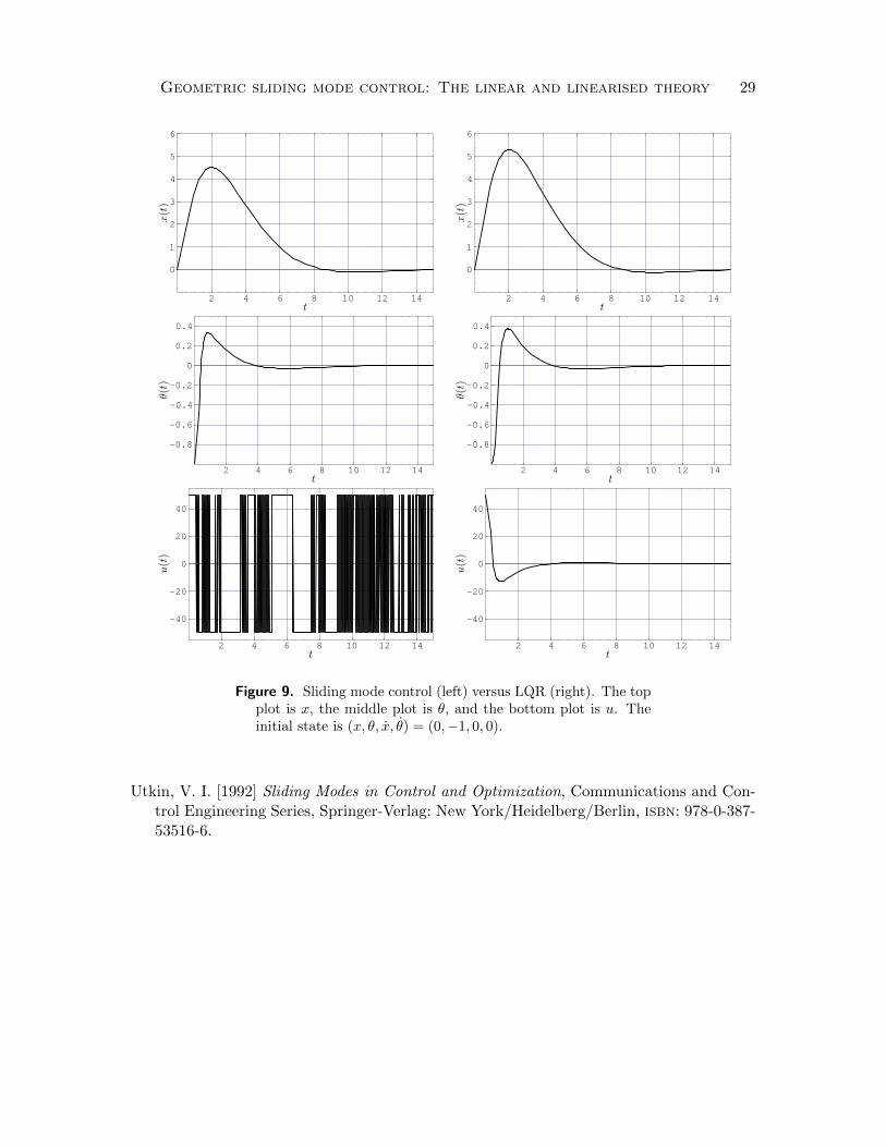
2 , and g = 9.81. The sliding mode controller uses the local control law ofSection 3.2 with K = 50. This value of K was chosen so that the maximum value of thesliding mode control law and the LQR control were roughly the same for the set of initialconditions simulated, cf. Figure 9. Note that there is not a radical difference in performanceof the two systems. The sliding mode controller works better for the initial condition closerto the equilibrium point. This is not surprising since it uses a larger maximum control effortthan the LQR controller is allowed.

7. Summary

In this paper we have provided a viewpoint for sliding mode control that emphasisesstructural aspects of the method different from those commonly emphasised. We saw inSection 2 that this leads to a simplification of the notion of what is accomplished by theequivalent control. Also, we saw in Section 2.4 that our way of looking at sliding modecontrol allowed a simple characterisation of all sliding mode controllers for a simple ex-ample. In Section 3 we considered the linear case, providing a characterisation of knownresults in our geometric setting. The matter of locally extending the linearisation methods


2 4 6 8 10 12 14

0

0.5

1

1.5

t

x(t)

2 4 6 8 10 12 14

0

0.5

1

1.5

t

x(t)

2 4 6 8 10 12 14

-0.4

-0.3

-0.2

-0.1

0

0.1

0.2

t

θ(t)

2 4 6 8 10 12 14

-0.4

-0.3

-0.2

-0.1

0

0.1

0.2

tθ(t)

2 4 6 8 10 12 14

-40

-20

0

20

40

t

u(t)

2 4 6 8 10 12 14

-40

-20

0

20

40

t

u(t)

Figure 8. Sliding mode control (left) versus LQR (right). The topplot is x, the middle plot is θ, and the bottom plot is u. Theinitial state is (x, θ, x, θ) = (0,− 1

2 , 0, 0).

to a neighbourhood of a linearly controllable equilibrium were systematically explored inSection 5. In future work, we will further illustrate the utility of our geometric approachby investigating approaches to extend local sliding submanifolds obtained by linearisationas in Section 5 to more global sliding submanifolds. We will also look at systems for whichit is not possible to design a sliding submanifold using the linearisation as a starting point.

References

Edwards, C. and Spurgeon, S. K. [1998] Sliding Mode Control, Theory and Applications,number 7 in Systems and Control Book Series, Taylor & Francis: London/New York/-Philadelphia/Singapore, isbn: 978-0-748-4060-12.

Slotine, J.-J. and Li, W. [1990] Applied Nonlinear Control, Prentice-Hall: Englewood Cliffs,NJ, isbn: 978-0-13-040890-7.


2 4 6 8 10 12 14

0

1

2

3

4

5

6

t

x(t)

2 4 6 8 10 12 14

0

1

2

3

4

5

6

t

x(t)

2 4 6 8 10 12 14

-0.8

-0.6

-0.4

-0.2

0

0.2

0.4

t

θ(t)

2 4 6 8 10 12 14

-0.8

-0.6

-0.4

-0.2

0

0.2

0.4

t

θ(t)

2 4 6 8 10 12 14

-40

-20

0

20

40

t

u(t)

2 4 6 8 10 12 14

-40

-20

0

20

40

t

u(t)

Figure 9. Sliding mode control (left) versus LQR (right). The topplot is x, the middle plot is θ, and the bottom plot is u. Theinitial state is (x, θ, x, θ) = (0,−1, 0, 0).

Utkin, V. I. [1992] Sliding Modes in Control and Optimization, Communications and Con-trol Engineering Series, Springer-Verlag: New York/Heidelberg/Berlin, isbn: 978-0-387-53516-6.

geometric sliding mode control: the linear and linearised ...andrew/notes/pdf/2002c.pdf ·...

Documents