Geometric networks based on Markov point processes with

applications to mobile sensor networks

David J Irons∗ and Jonathan Jordan∗

Abstract

This paper presents a Markov point process model for generating geometric graphs, capable ofevolving over time and responding to external effects. Networks, from these models, are capable ofself organising to appropriately cover a space despite a variety of obstacles or geographical constraints.These models have direct applications to mobile sensor networks, made up of mobile computationalunits capable of local environmental sensing and communication. In line with the desirable propertiesand deployment challenges for these systems, we evaluate summary statistics for our models; such ascoverage, connectivity and robustness. We also demonstrate and evaluate how our models are applicableon three dimensional geographical terrains.

Key words and phrases: mobile sensor networks, geometric graph, Markov point processes, self-organisation.

AMS 2010 subject classification: Primary 68M10; secondary 05C90, 60D05, 60G55, 65C05.

1 Introduction

In random geometric graphs, a set of vertices are randomly distributed in geometric space and edges arethen added between them based on some geometrical constraint. For example, in the standard randomgeometric graph model described in Penrose [11], edges exist between any pair of vertices within distanceR of one another (Figure 1A, 2A). Other models based on vertices distributed randomly in space includethe SERN models of Barnett et al [4] and the proximity graphs, such as the Gabriel graph, described inAldous and Shun [1]. Due to the fact that these models explicitly take into account space, they have a widerange of applications, including biological networks, epidemic modelling and communication networks; seethe introduction to Penrose [11].

One application of particular interest here is wireless sensor networks (for reviews see Kiess and Mauve [8],Ghosh and Das [5] and Yick et al [17]). Here, sensors capable of local wireless communication are spatiallydistributed to monitor environmental features such as heat, light, hazardous chemicals or motion. Althoughstill a developing field, applications include environment monitoring, target tracking and monitoring ofhazardous material. Sensor networks face a wide range of challenges such as network coverage, routingand energy efficiency, see for example Puccinelli and Haenggi [12], Ghosh and Das [5], Younis and Akkaya[18] and Anastasi et al [2]. The individual computational units may be fragile, have limited lifespanand only be able to communicate locally. Moreover, the environments may be hostile, poorly understoodand changeable over time. However, despite these individual restrictions, they still need to be able toself-organise to produce a robust and reliable network that covers the whole environment.

∗School of Mathematics and Statistics, University of Sheffield, Hounsfield Road, Sheffield S3 7RH

1

Traditionally, geometric graph models in this area have assumed a static arrangement of vertices, witheach vertex capable of sensing and communicating within radii RS and RC respectively. However, withadvancements in robotics there is also a growing interest in mobile sensor networks that are capableof movement around their environment. Therefore, there is also currently a need to develop advancedmodels that incorporate dynamic features such as vertex movement, edge re-wiring and differential vertexbehaviour.

In this paper, we aim to use the theory of Markov point processes, described in van Lieshout [14], to obtaina more efficient configuration of the vertices of the network in space. We adapt Markov Chain Monte Carlo(MCMC) methods for simulating from Markov point processes, which are described in [14]. In particular,we provide a method which uses movements of the vertices to improve the configuration of the vertices,starting from a random (or other) configuration in space. We will discuss the theory of Markov pointprocesses in more detail in section 2.

Due to the dynamic nature of these models, we show how they can be applied to mobile sensor networks;in particular the challenge of ensuring the resulting networks provide good coverage of the environment ofinterest. We also show that coverage is robust against vertex failure, initial vertex placement and obstaclesin the space of interest. Moreover, we show that our models are applicable to more realistic 3D terrains,which can dramatically affect the communication links (edges) between vertices.

A number of existing papers have also used graph models to study the coverage problem, when deployingvertices in mobile sensor networks. A number of groups have employed deterministic models that userepulsive forces between vertices (and obstacles) to move close vertices away from one another and generatean even spread; see Howard et al [7], Zou and Chakrabarty [19], Wang et al [15] and Heo and Varshney [6].In some cases, attractive forces are also used to pull vertices towards areas requiring coverage (e.g. [15, 19]).However, these algorithms are primarily deterministic and rely on the co-ordinates of each vertex beingknown (or at least the distances and orientations between every pair of vertices being known). Meanwhile,stochastic models for vertex movement have been employed when considering coverage over a period oftime; see Liu et al [9], Winfield [16] and Sinclair and Stauffer [13]. However, these assume purely randommovement of vertices, which does not achieve the even distribution of vertices that the above mentionedmodels do.

Our work shares some features with the above mentioned models, due to the fact that repulsive andattractive mechanisms are used to generate vertex movement. However, our work differs due the fact thatthis is a probabilistic model that does not depend on the precise location of vertices. Rather, only localinformation is required about the distances between pairs of vertices, which makes network generationmore realistic when vertex communication and localisation is unreliable. Moreover, we specifically look atrealistic 3D terrains and ‘line of sight’ communications when evaluating our models.

In section 2 and 3 we define our model and provide some simple examples on both flat and 3D terrains.Within these sections we also consider how the model is able to adapt to obstacles and the initial placementof vertices. Section 4 then analyses the evolution of the resulting network structures over time. We thenfurther discuss our work in the context of mobile sensor networks in section 5.

2 Models and Markov point processes

In this section we introduce the family of Markov point processes which our method is based on anddescribe the methods for simulating them, following van Lieshout [14].

We are interested in situations where we have a fixed number n of vertices which are to be given locations

2

Figure 1: (A) Example for geometric graph connections where 2 vertices are connected if within radius r2of one another (B) Example of preferential movement. Grey vertices are more likely to move towards/awayfrom the black vertex if the new position is within distance r2 (solid)/beyond distance r1 (dashed). (C)Example for line of sight constraint, whereby vertices can’t connect (dotted line) if a hill obscures the viewbetween them.

A B C

in some space D (giving a configuration X ). We wish to form a geometric graph, defined as in Penrose[11] to mean the graph G(X , r2) formed by connecting vertices if and only if the distance (Euclidean)between them is less than r2 (thought of as a communication radius). If the vertices in X are obtained byconditioning a Poisson point process to have exactly n points then we obtain random geometric graphs inthe sense of Penrose [11] (e.g. Figure 2A (top)).

We wish to ensure that the locations of the vertices give good coverage of D, in the sense that an eventhappening at any location within D can be detected by a nearby vertex and its occurrence communicatedto the rest of the network. We also aim to ensure good coverage by having few pairs of vertices withinr1 of each other, where r1 < r2. In particular we aim to improve on the coverage obtained from randomgeometric graphs based on Poisson point processes.

The general method is to allow the vertices to move according to rules based on the Metropolis-Hastingsalgorithm for simulating Markov point processes, described in van Lieshout [14]. This can give a set ofsimple rules which, if run for enough steps, will give a random pattern of points with a distribution closeto that of the Markov point process. The set of rules aim to ensure that vertices within distance r1 arerepelled from one another, whilst maintaining edges between vertices that are within distance d ∈ (r1, r2)(Fig 1B). We aim to choose the Markov point process in a suitable way.

2.1 Markov point processes

The point processes we are interested in are examples of Ripley-Kelly Markov point processes, as definedin van Lieshout [14], and we will concentrate on pairwise interaction processes.

To define these we need to define a ‘neighbourhood’ relationship ∼ on D; we will use the relationship thatu ∼ v if and only if d(u, v) ≤ R.

We can then define the pairwise interaction processes that we are interested in via a density

p(x) = α∏

ξ,η∈x,ξ∼η

ϕ(ξ, η).

Here x is a possible configuration of n vertices, ϕ is a function describing the interaction between ‘neigh-

3

bouring’ vertices, and α is a normalising constant.

Choosing different forms for ϕ(ξ, η) allows us to incorporate interactions between points, for example wecan incorporate repulsion between vertices which are too close together, by making ϕ(ξ, η) small if distanced(ξ, η) is small. A particularly simple example is the Strauss process, described in van Lieshout [14], whichproduces a random pattern of vertices with inhibition within a distance r1. There is a parameter γ; ifγ = 0 the inhibition is total and if γ = 1 there is no inhibition (i.e. we have a Poisson process). In theabove framework, R = r1 and ϕ(ξ, η) = γ.

We propose to allow for greater inhibition the closer vertices are together (rather than a step function asin the Strauss process), by working with a pairwise interaction Markov point process with potential

ϕ({ξ, η}) = γI{d(ξ,η)<r1}r1

d(ξ,η) , (1)

where γ < 1 and I{d(ξ,η)<r1} is the indicator function returning 1 if the condition d(ξ, η) < r1 is true (0otherwise). This potential provides a repulsive effect if two vertices are closer than r1 apart, which getsstronger the closer they are together.

In some circumstances it is useful to have an extra factor in the potential which provides an attractiveterm when vertices are close enough to be connected; this makes it less likely that vertices will be poorlyconnected in the network. This uses a parameter δ ≥ 1, and we have a pairwise interaction Markov pointprocess with potential

ϕ({ξ, η}) = γI{d(ξ,η)<r1}r1

d(ξ,η) δI{d(ξ,η)<r2} , (2)

providing (if δ > 1) a high potential if vertices are within r2 but not too close together. The potential in(1) is recovered if δ = 1.

We can now use the following simulation method, based on Metropolis-Hastings MCMC methods forsimulating Strauss processes conditioned on having exactly n points (see van Lieshout [14] and Andersson[3]) and designed so that the method can be implemented with only local knowledge. For clarity, weinitially describe the method in the case δ = 1 and the space D being the unit square.

1. At each time step a vertex is chosen, uniformly at random, for a possible move

2. The direction of the move is chosen at random from a uniform distribution on [0, 2π] and the distanceto move is chosen from a distribution on [0, r3], where r3 = r2−r1. In the simulations the distributionfor the moves is a Beta distribution scaled to have support [0, r3].

3. If the move takes the vertex out of the unit square, it is rejected.

4. For the chosen vertex position xv, we calculate

nO =∑i =v

I{d(xv,xi)<r1}r1

d(xv, xi)

and, where xN is the proposed new location, let

nN =∑i =v

I{d(xN ,xi)<r1}r1

d(xN , xi).

5. The move is then “accepted” with probability min(1, γnN−nO ) (where γ is a the parameter introducedin (1)).

4

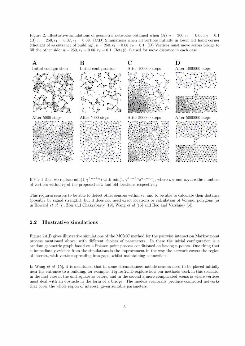
Figure 2: Illustrative simulations of geometric networks obtained when (A) n = 300, r1 = 0.05, r2 = 0.1(B) n = 250, r1 = 0.07, r2 = 0.08. (C,D) Simulations when all vertices initially in lower left hand corner(thought of as entrance of building); n = 250, r1 = 0.06, r2 = 0.1. (D) Vertices must move across bridge tofill the other side; n = 250, r1 = 0.06, r2 = 0.1. Beta(5, 1) used for move distance in each case

A B C DInitial configuration Initial configuration After 100000 steps After 1000000 steps

After 5000 steps After 5000 steps After 500000 steps After 5000000 steps

If δ > 1 then we replace min(1, γnN−nO ) with min(1, γnN−nOδnN−nO ), where nN and nO are the numbersof vertices within r2 of the proposed new and old locations respectively.

This requires sensors to be able to detect other sensors within r2, and to be able to calculate their distance(possibly by signal strength), but it does not need exact locations or calculation of Voronoi polygons (asin Howard et al [7], Zou and Chakrabarty [19], Wang et al [15] and Heo and Varshney [6]).

2.2 Illustrative simulations

Figure 2A,B gives illustrative simulations of the MCMC method for the pairwise interaction Markov pointprocess mentioned above, with different choices of parameters. In these the initial configuration is arandom geometric graph based on a Poisson point process conditioned on having n points. One thing thatis immediately evident from the simulations is the improvement in the way the network covers the regionof interest, with vertices spreading into gaps, whilst maintaining connections.

In Wang et al [15], it is mentioned that in some circumstances mobile sensors need to be placed initiallynear the entrance to a building, for example. Figure 2C,D explore how our methods work in this scenario,in the first case in the unit square as before, and in the second a more complicated scenario where verticesmust deal with an obstacle in the form of a bridge. The models eventually produce connected networksthat cover the whole region of interest, given suitable parameters.

5

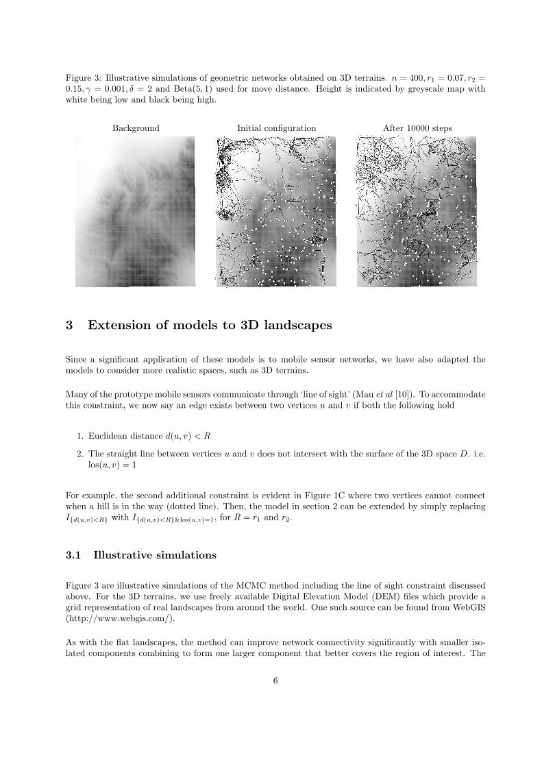
Figure 3: Illustrative simulations of geometric networks obtained on 3D terrains. n = 400, r1 = 0.07, r2 =0.15, γ = 0.001, δ = 2 and Beta(5, 1) used for move distance. Height is indicated by greyscale map withwhite being low and black being high.

Background Initial configuration After 10000 steps

3 Extension of models to 3D landscapes

Since a significant application of these models is to mobile sensor networks, we have also adapted themodels to consider more realistic spaces, such as 3D terrains.

Many of the prototype mobile sensors communicate through ‘line of sight’ (Mau et al [10]). To accommodatethis constraint, we now say an edge exists between two vertices u and v if both the following hold

1. Euclidean distance d(u, v) < R

2. The straight line between vertices u and v does not intersect with the surface of the 3D space D. i.e.los(u, v) = 1

For example, the second additional constraint is evident in Figure 1C where two vertices cannot connectwhen a hill is in the way (dotted line). Then, the model in section 2 can be extended by simply replacingI{d(u,v)<R} with I{d(u,v)<R}&los(u,v)=1, for R = r1 and r2.

3.1 Illustrative simulations

Figure 3 are illustrative simulations of the MCMC method including the line of sight constraint discussedabove. For the 3D terrains, we use freely available Digital Elevation Model (DEM) files which provide agrid representation of real landscapes from around the world. One such source can be found from WebGIS(http://www.webgis.com/).

As with the flat landscapes, the method can improve network connectivity significantly with smaller iso-lated components combining to form one larger component that better covers the region of interest. The

6

anonymised example shown contains a number of geographical features, such as flat plains, hills and valleys.Due to the fact that hill peaks can prevent connections, vertices tend to form most connections throughvalleys or on hill slopes. Meanwhile, relatively flat areas (top left) tend to lead to similar behaviour to flatlandscapes. This is typical of a number of landscapes investigated (results not shown).

4 Evolution of summary statistics

When formally assessing network structure and coverage in our models, we use a number of summarystatistics.

In terms of network connectivity , we are interested in

Definition 1. (a) The largest connected component : the largest subgraph V ⊂ G, such that every vertexcan be reached by every other vertex, by following network edges

(b) The degree of a vertex u: the number of vertices connected to u

(c) The shortest path length between two vertices u and v: the number of edges in the shortest pathconnecting them

In terms of the shortest path length, we score networks based on

‘observed average shortest path length − expected average path length’.

Here, the expected value is based on random geometric graphs with the same size largest component.

In terms of coverage, noting Heo and Varshney [6], we are interested in

Definition 2. The coverage of a (connected) graph is

C =∪i=1,...,NAi

A

where

Ai is the area covered by the ith vertex

N is the total number of vertices

A is the area of the whole space D

In the case considered here, individual vertices can cover a disc of radius r2, centered on themselves.

Definition 3. The irregularity of a (connected) graph is

U =1

N

∑Ni=1 Ui

7

where

Ui =

(1

Ki

∑Ki

j=1(d(i, j)−Mi)2

)1

2

and

Ki is the number of neighbours of the ith vertex

N is the total number of vertices

d(i, j) is the distance between ith and jth vertices

Mi is the mean of internodal distances between the ith vertex and its neighbours

Measures of robustness are also of interest such as how connectivity and coverage are affected by randomvertex death or random edge/communication failures.

4.1 Summary statistics on flat landscapes

We start by looking at the evolution of the network over time when working with the model of section 2 ona unit square, and beginning with a random geometric graph (Figures 4 and 5). For a small/large numberof vertices the networks are sparse/well connected respectively (and similarly for small/large radius ofconnectivity r2). Therefore, we chose n = 120, r1 = 0.05 and r2 = 0.1 to consider the transitional scenariobetween the two. When δ = 1 (so that we only have repulsion), the size of and coverage by the largestcomponent increase over time (Figure 4A,B), demonstrating improved performance over random geometricgraphs (t = 0). The distribution of edge lengths also became more regular as vertices spread more evenlyacross the space (Figure 5C). However, other connectivity measures deteriorate when δ = 1, with theaverage degree decreasing and shortest path lengths increasing beyond the expected length (Figure 5A,4C).

We also considered how the process performed as the number of initial vertices increased (Figure 6, 7).As would be expected, many of the above mentioned statistical measures improved as the number ofvertices increased. In particular the size of the largest component, average degree (in largest component)and area covered by largest component all increase as the number of vertices increase. An exception tothis is the distribution of edge lengths (Figure 7C), which become more variable. This is due to the factthat as vertices become closer together (average distance approaching r1) edges form over a wider range ofdistances between r1 and r2. Finally, the situation with shortest path length (Figure 6C) is often dependenton other parameters, but tends to improve (score decreases) for a moderate number of vertices. However,for a large number of vertices the score converges back to 0, since there is no improvement over randomgeometric graphs in this case.

We have also investigated how the repulsion and attraction parameters (γ and δ respectively) affect connec-tivity and coverage statistics. For the process to work effectively γ needs to be small but, beyond that, theprocess is reasonably insensitive to the choice. For the simulations here we chose γ = 0.001. Meanwhile,the performance was particularly sensitive to δ, the parameter controlling how much vertices are attractedto one another when moving (δ = 1 implies no attraction). In the flat scenario (unit square) at least,increasing δ led to improvements in network connectivity as the largest component grew, vertex degreeincreased and shortest path length decreased (Figures 4–7). However, the distribution of edge lengths

8

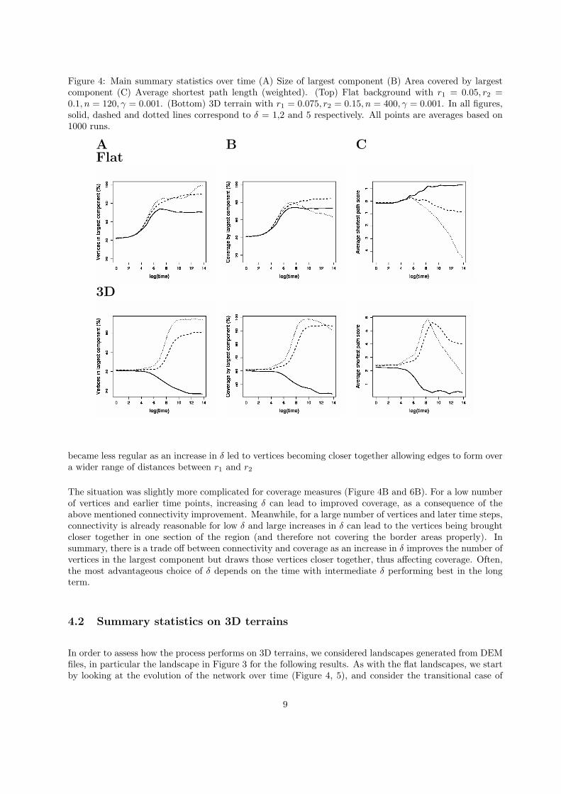
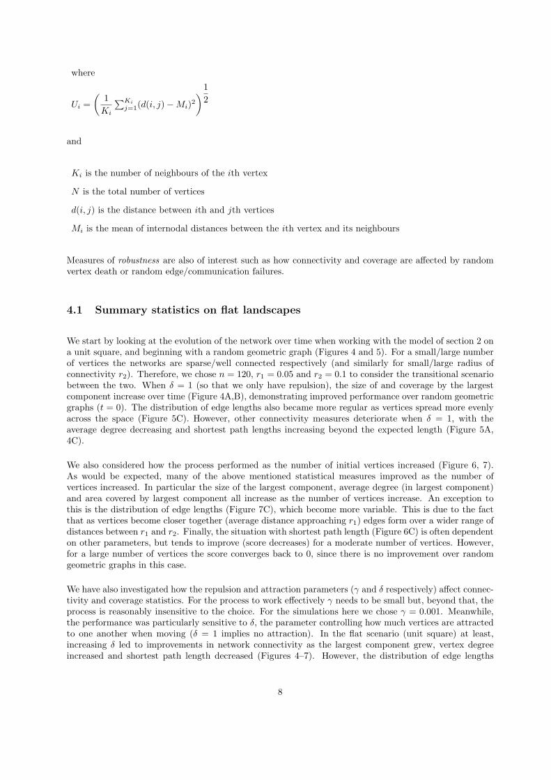
Figure 4: Main summary statistics over time (A) Size of largest component (B) Area covered by largestcomponent (C) Average shortest path length (weighted). (Top) Flat background with r1 = 0.05, r2 =0.1, n = 120, γ = 0.001. (Bottom) 3D terrain with r1 = 0.075, r2 = 0.15, n = 400, γ = 0.001. In all figures,solid, dashed and dotted lines correspond to δ = 1,2 and 5 respectively. All points are averages based on1000 runs.

A B CFlat

3D

became less regular as an increase in δ led to vertices becoming closer together allowing edges to form overa wider range of distances between r1 and r2

The situation was slightly more complicated for coverage measures (Figure 4B and 6B). For a low numberof vertices and earlier time points, increasing δ can lead to improved coverage, as a consequence of theabove mentioned connectivity improvement. Meanwhile, for a large number of vertices and later time steps,connectivity is already reasonable for low δ and large increases in δ can lead to the vertices being broughtcloser together in one section of the region (and therefore not covering the border areas properly). Insummary, there is a trade off between connectivity and coverage as an increase in δ improves the number ofvertices in the largest component but draws those vertices closer together, thus affecting coverage. Often,the most advantageous choice of δ depends on the time with intermediate δ performing best in the longterm.

4.2 Summary statistics on 3D terrains

In order to assess how the process performs on 3D terrains, we considered landscapes generated from DEMfiles, in particular the landscape in Figure 3 for the following results. As with the flat landscapes, we startby looking at the evolution of the network over time (Figure 4, 5), and consider the transitional case of

9

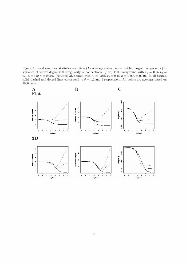
Figure 5: Local summary statistics over time (A) Average vertex degree (within largest component) (B)Variance of vertex degree (C) Irregularity of connections. (Top) Flat background with r1 = 0.05, r2 =0.1, n = 120, γ = 0.001. (Bottom) 3D terrain with r1 = 0.075, r2 = 0.15, n = 400, γ = 0.001. In all figures,solid, dashed and dotted lines correspond to δ = 1,2 and 5 respectively. All points are averages based on1000 runs.

A B CFlat

3D

10

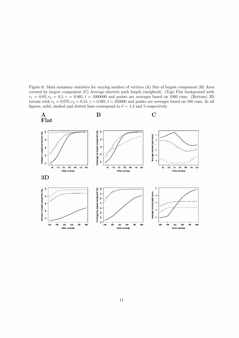
Figure 6: Main summary statistics for varying number of vertices (A) Size of largest component (B) Areacovered by largest component (C) Average shortest path length (weighted). (Top) Flat background withr1 = 0.05, r2 = 0.1, γ = 0.001, t = 1000000 and points are averages based on 1000 runs. (Bottom) 3Dterrain with r1 = 0.075, r2 = 0.15, γ = 0.001, t = 250000 and points are averages based on 100 runs. In allfigures, solid, dashed and dotted lines correspond to δ = 1,2 and 5 respectively

A B CFlat

3D

11

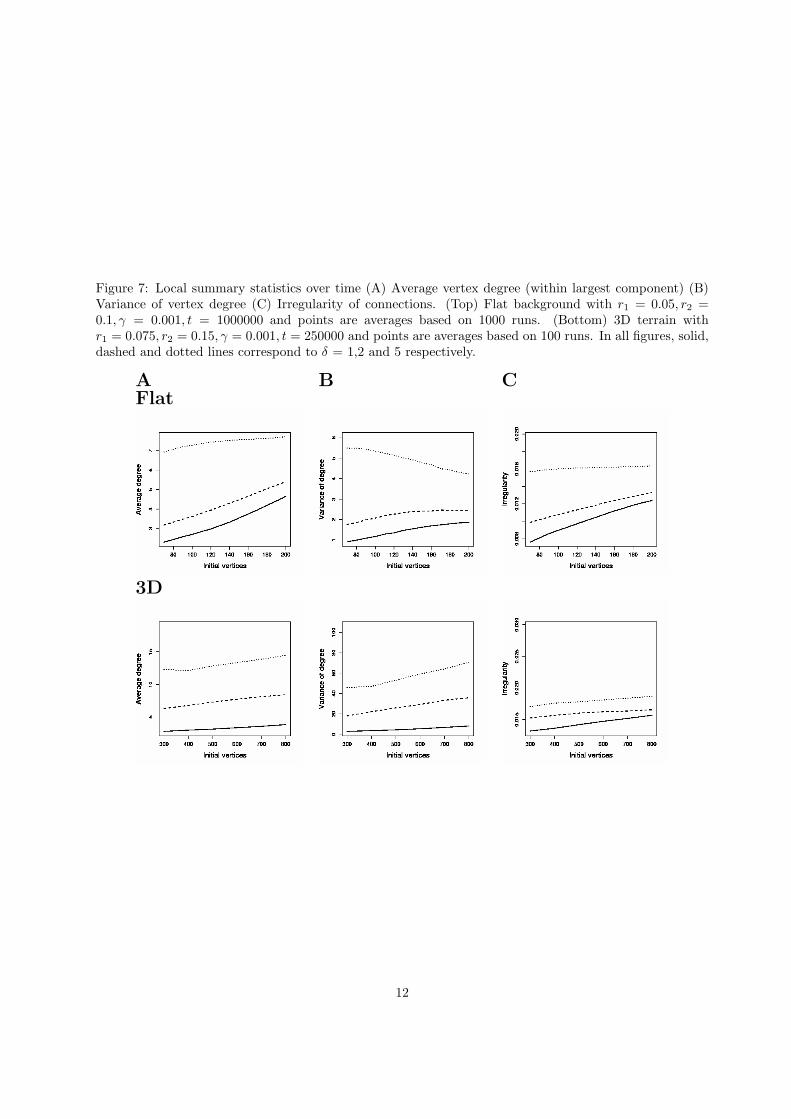
Figure 7: Local summary statistics over time (A) Average vertex degree (within largest component) (B)Variance of vertex degree (C) Irregularity of connections. (Top) Flat background with r1 = 0.05, r2 =0.1, γ = 0.001, t = 1000000 and points are averages based on 1000 runs. (Bottom) 3D terrain withr1 = 0.075, r2 = 0.15, γ = 0.001, t = 250000 and points are averages based on 100 runs. In all figures, solid,dashed and dotted lines correspond to δ = 1,2 and 5 respectively.

A B CFlat

3D

12

n = 400, r1 = 0.075 and r2 = 0.15 where networks are neither very sparse nor very well connected.

This time, when δ =1 (so that we only have repulsion), the largest component and the area covered by itdecreased over time (Figure 4A,B). This is since the additional geographical constraints, combined with therepulsion mechanism, cause the network to break into smaller geographically isolated components. Indeedthe largest component tends only to cover a small region (in this case the flat section in the top left of Figure3). The largest component being restricted to flat sections of the landscape also explains the observed dropin average degree and edge length irregularity (Figure 5), in line with that observed for flat landscapes.Once again the attraction parameter δ dramatically affects the results. Just a small increase in δ tended tomake the resulting networks much better connected and able to cover the majority of the region of interest(Figure 4A,B). This increase in connectivity is also demonstrated by an increase in average degree (Figure5). However, as with the flat landscape, setting δ too high can lead to a deterioration in coverage in thelong term (δ = 5 in Figure 4B). For increased δ, the average shortest path length also showed some bigincreases for intermediate time steps. This is due to most of the paths now having to follow valleys, ratherthan cross hills to maintain network connectivity (Figure 4C).

We also considered how the process performed as the number of initial vertices increased (Figure 6, 7).As with the flat landscapes, most statistical measures improved as the number of vertices increased, withthe size of the largest component and the area covered by it increasing. Meanwhile average degree andedge length irregularity show moderate increases and so there is no qualitative difference from the flatlandscapes (Figure 7). In the 3D case considered, the attraction parameter δ was again significant, indeed,more so than in the case of flat landscapes, with the largest component, vertex degree and coverage allsignificantly increasing with only a small increase in δ (1 to 2). The value of δ affected average shortestpath length differently for small and large number of vertices. This is due to the fact that when n andδ are small, the largest component is restricted to the flatter sections of the landscape and the resultingsub-network is fairly regular. When n or δ are large, networks cover more of the region and are less regularas they cut through valleys etc. Therefore, the results are biased by the size and spread of the largestcomponent.

4.3 Robustness to vertex and communication failure

Another property of interest, from both a theoretical and application viewpoint, is robustness to errors.

We first considered how the process performed when vertices randomly die over time. In Figure 8, weshow how a number of statistical measures are affected by vertex death (when n = 160). Here, the xaxis is the probability p that a vertex dies at some (randomly chosen) time during the process. The plotsshow the properties of the networks at the end of the process (t = 1000000 steps), whilst the additionalpoints show the comparison case where the process started with n(1−p) vertices (but there was no death).Overall, the process is remarkably robust, compared to the case where we just start with an equivalentnumber of live vertices (Figure 8); especially for moderate vertex death rates. However, when the attractionparameter δ is 1 (no attraction between neighbouring vertices), high death rates can lead to a deteriorationin connectivity and coverage. Meanwhile, this is not the case for higher values of δ, and so it appears thatincreasing attraction (via δ) can help reconnect the network in response to vertex death and so increaserobustness.

Secondly, we considered how the process performed to communication/edge errors. During the process,movement decisions are based on the distances between pairs of vertices. In Figure 9, we assumed thatpairs of vertices fail to calculate this distance with probability p (independently at every time step). Wethen calculated how a number of statistical measures are affected by communication failure as before (whenn = 120). All of the cases shown are relatively robust, in sense that communication errors only lead togradual deterioration in the connectivity and coverage of the network. Similar to earlier results, increasing

13

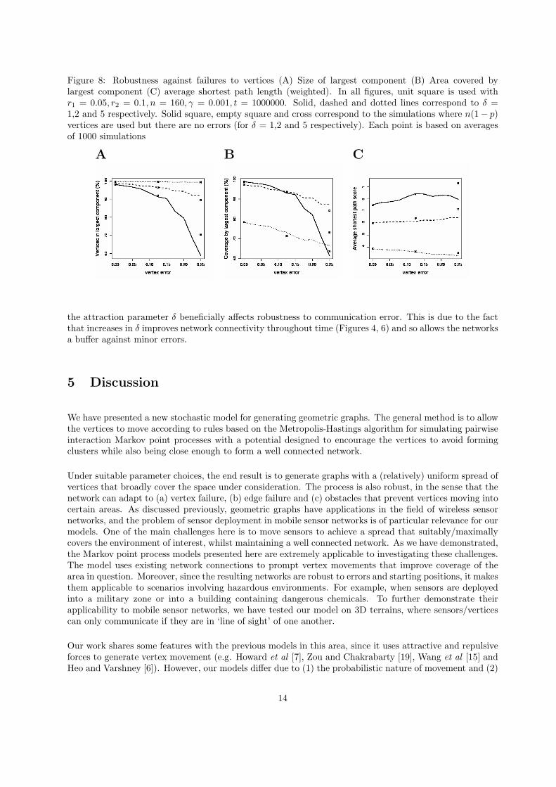
Figure 8: Robustness against failures to vertices (A) Size of largest component (B) Area covered bylargest component (C) average shortest path length (weighted). In all figures, unit square is used withr1 = 0.05, r2 = 0.1, n = 160, γ = 0.001, t = 1000000. Solid, dashed and dotted lines correspond to δ =1,2 and 5 respectively. Solid square, empty square and cross correspond to the simulations where n(1− p)vertices are used but there are no errors (for δ = 1,2 and 5 respectively). Each point is based on averagesof 1000 simulations

A B C

the attraction parameter δ beneficially affects robustness to communication error. This is due to the factthat increases in δ improves network connectivity throughout time (Figures 4, 6) and so allows the networksa buffer against minor errors.

5 Discussion

We have presented a new stochastic model for generating geometric graphs. The general method is to allowthe vertices to move according to rules based on the Metropolis-Hastings algorithm for simulating pairwiseinteraction Markov point processes with a potential designed to encourage the vertices to avoid formingclusters while also being close enough to form a well connected network.

Under suitable parameter choices, the end result is to generate graphs with a (relatively) uniform spread ofvertices that broadly cover the space under consideration. The process is also robust, in the sense that thenetwork can adapt to (a) vertex failure, (b) edge failure and (c) obstacles that prevent vertices moving intocertain areas. As discussed previously, geometric graphs have applications in the field of wireless sensornetworks, and the problem of sensor deployment in mobile sensor networks is of particular relevance for ourmodels. One of the main challenges here is to move sensors to achieve a spread that suitably/maximallycovers the environment of interest, whilst maintaining a well connected network. As we have demonstrated,the Markov point process models presented here are extremely applicable to investigating these challenges.The model uses existing network connections to prompt vertex movements that improve coverage of thearea in question. Moreover, since the resulting networks are robust to errors and starting positions, it makesthem applicable to scenarios involving hazardous environments. For example, when sensors are deployedinto a military zone or into a building containing dangerous chemicals. To further demonstrate theirapplicability to mobile sensor networks, we have tested our model on 3D terrains, where sensors/verticescan only communicate if they are in ‘line of sight’ of one another.

Our work shares some features with the previous models in this area, since it uses attractive and repulsiveforces to generate vertex movement (e.g. Howard et al [7], Zou and Chakrabarty [19], Wang et al [15] andHeo and Varshney [6]). However, our models differ due to (1) the probabilistic nature of movement and (2)

14

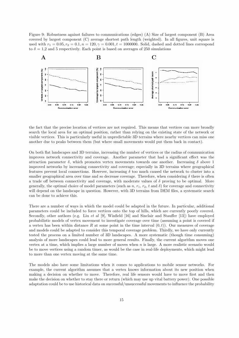
Figure 9: Robustness against failures to communications (edges) (A) Size of largest component (B) Areacovered by largest component (C) average shortest path length (weighted). In all figures, unit square isused with r1 = 0.05, r2 = 0.1, n = 120, γ = 0.001, t = 1000000. Solid, dashed and dotted lines correspondto δ = 1,2 and 5 respectively. Each point is based on averages of 250 simulations

A B C

the fact that the precise location of vertices are not required. This means that vertices can more broadlysearch the local area for an optimal position, rather than relying on the existing state of the network orvisible vertices. This is particularly useful in unpredictable 3D terrains where nearby vertices can miss oneanother due to peaks between them (but where small movements would put them back in contact).

On both flat landscapes and 3D terrains, increasing the number of vertices or the radius of communicationimproves network connectivity and coverage. Another parameter that had a significant effect was theattraction parameter δ, which promotes vertex movements towards one another. Increasing δ above 1improved networks by increasing connectivity and coverage; especially in 3D terrains where geographicalfeatures prevent local connections. However, increasing δ too much caused the network to cluster into asmaller geographical area over time and so decrease coverage. Therefore, when considering δ there is oftena trade off between connectivity and coverage, with moderate values of δ proving to be optimal. Moregenerally, the optimal choice of model parameters (such as n, r1, r2, t and δ) for coverage and connectivitywill depend on the landscape in question. However, with 3D terrains from DEM files, a systematic searchcan be done to achieve this.

There are a number of ways in which the model could be adapted in the future. In particular, additionalparameters could be included to force vertices onto the top of hills, which are currently poorly covered.Secondly, other authors (e.g. Liu et al [9], Winfield [16] and Sinclair and Stauffer [13]) have employedprobabilistic models of vertex movement to investigate coverage over time (assuming a point is covered ifa vertex has been within distance R at some point in the time interval (0, t)). Our measures of coverageand models could be adapted to consider this temporal coverage problem. Thirdly, we have only currentlytested the process on a limited number of 3D landscapes. A more systematic (though time consuming)analysis of more landscapes could lead to more general results. Finally, the current algorithm moves onevertex at a time, which implies a large number of moves when n is large. A more realistic scenario wouldbe to move vertices using a random timer, as would be the case in real-life deployments, which might leadto more than one vertex moving at the same time.

The models also have some limitations when it comes to applications to mobile sensor networks. Forexample, the current algorithm assumes that a vertex knows information about its new position whenmaking a decision on whether to move. Therefore, real life sensors would have to move first and thenmake the decision on whether to stay there or return (which may use up vital battery power). One possibleadaptation could be to use historical data on successful/unsuccessful movements to influence the probability

15

of directions for future movements. Information on the connectivity of neighbouring vertices could also beused.

Acknowledgements

We thank Chris Cannings, Fabrice Saffre and Paul Blackwell for helpful discussions. We also thank NingMa for help with network simulations. This work was supported by EPSRC grant EP/D003105/1.

References

[1] D. Aldous and J. Shun. Connected spatial networks over random points and a route-length statistic.Preprint, avaiable from http://arxiv.org/abs/1003.3700, 2010.

[2] G. Anastasi, M. Conti, M. Di Francesco, and A. Passarella. Energy conservation in wireless sensornetworks: A survey. Ad Hoc Networks, 7:537–568, 2009.

[3] J. Andersson. Mcmc simulation of markov point processes. Available from http://www.math.

chalmers.se/~olleh/Markov_Andersson.pdf, 2005.

[4] L. Barnett, E. Di Paolo, and S. Bullock. Spatially embedded random networks. Phys. Rev. E,76:056115, 2007.

[5] A. Ghosh and S.K. Das. Coverage and connectivity issues in wireless sensor networks: A survey. Perv.and Mob. Comp., 4:303–334, 2008.

[6] N. Heo and P.K. Varshney. Energy-efficient deployment of intelligent mobile sensor networks. IEEETransactions on Systems, Man and Cybernetics - Part A, 35:78–92, 2005.

[7] A. Howard, M.M Mataric, and G.S. Sukhatme. Mobile sensor network deployment using potentialfields: A distributed, scalable solution to the area coverage problem. Proceedings of the 6th Interna-tional Symposium on Distributed Autonomous Robotic Systems (DARS02), Fukuoka, Japan, 2002.

[8] W. Kiess and M. Mauve. A survey on real-world implementations of mobile ad-hoc networks. Ad HocNetworks, 5:324–339, 2007.

[9] B. Liu, P. Brass, O. Dousse, P. Nain, and D. Towsley. Mobility improves coverage of sensor networks.Proceedings of MOBIHOC, Urbana-Champaign, 2005.

[10] G. Mao, B. Fidan, and B.D.O. Anderson. Wireless sensor network localization techniques. ComputerNetworks, 51:2529–2553, 2007.

[11] M. Penrose. Random geometric graphs. Oxford University Press, 2003.

[12] D. Puccinelli and M. Haenggi. Wireless sensor networks: Applications and challenges of ubiquitoussensing. IEEE Circuits and Systems Magazine, 5:19–31, 2005.

[13] A. Sinclair and A. Stauffer. Mobile geometric graphs, and detection and communication problems inmobile wireless networks. Preprint. Available from http://arxiv.org/abs/1005.1117, 2010.

[14] M. N. M. van Lieshout. Markov Point Processes and their applications. Imperial College Press, 2000.

[15] G. Wang, G. Cao, and T. La Porta. Movement-assisted sensor deployment. Proceedings of the 23rdInternational Annual Joint Conference of the IEE Computer and Communications Societies (INFO-COM’04), Hong Kong, 2004.

16

[16] A.F.T. Winfield. Distributed sensing and data collection via broken ad hoc wireless connected networksof mobile robots. Distributed Autonomous Robots 4, Eds L.E. Parker and G. Bekey and J. Barhen,New York: Springer-Verlag, 2000.

[17] J. Yick, B. Mukherjee, and D. Ghosal. Wireless sensor network survey. Computer Networks, 52:2292–2330, 2008.

[18] M. Younis and K. Akkaya. Strategies and techniques for node placement in wireless sensor networks:A survey. Ad Hoc Networks, 6:621–655, 2008.

[19] Y. Zou and K. Chakrabarty. Sensor deployment and target localization in distributed sensor networks.ACM Transactions on Embedded Computing Systems (TECS), 3:61 – 91, 2004.

17