geometric data structures for computer graphics - gabriel zachmann
TRANSCRIPT

EUROGRAPHICS 2002 Tutorial
Geometric Data Structures for Computer Graphics
Gabriel Zachmann and Elmar Langetepe
Informatik II/IUniversity of Bonn
Römerstr. 16453111 Bonn, Germany
email: zach,[email protected]://web.cs.uni-bonn.de/~zach
http://web.cs.uni-bonn.de/I/staff/langetepe.html
© The Eurographics Association 2002.

2 Zachmann and Langetepe / Geometric Data Structures for CG
Contents1 Introduction
2 Quadtrees and K-d-Trees
2.1 Quadtrees and Octrees
2.2 K-d-Trees
2.3 Height Field Visualization
2.4 Isosurface Generation
2.5 Ray Shooting
3 BSP Trees
3.1 Rendering Without a Z-Buffer
3.2 Representing Objects with BSPs
3.3 Boolean Operations
4 Bounding Volume Hierarchies
4.1 Construction of BV Hierarchies
4.2 Collision Detection
5 Voronoi Diagrams
5.1 Definitions and Elementary Properties
5.2 Computation
5.3 Generalization of the Voronoi Diagram
5.4 Applications of the Voronoi Diagram
5.5 Texture Synthesis
5.6 Shape Matching
6 Dynamization of Geometric Data Structures
6.1 Model of the Dynamization
6.2 Amortized Insert and Delete
6.3 Worst-Case sensitive Insert and Delete
6.4 A Simple Example
References
© The Eurographics Association 2002.

Zachmann and Langetepe / Geometric Data Structures for CG 3
AbstractThe goal of this tutorial is to present a wide range of geometric data structures, algorithms and techniquesfrom computational geometry to computer graphics practitioners. To achieve this goal we introduce severaldata structures, discuss their complexity, point out construction schemes and the corresponding performanceand present standard applications in two and three dimensions.
Categories and Subject Descriptors (according to ACM CCS): Categories and Subject Descriptors: I.3.3 [DataStructures]: Computer Graphics
1 IntroductionIn recent years, methods from computational geometryhave been widely adopted by the computer graphics com-munity. Many solutions draw their elegance and efficiencyfrom the mutually enriching combination of such geomet-rical data structures with computer graphics algorithms.
With this tutorial we try to familiarize practitioners inthe computer graphics field with several geometric datastructures, algorithms and techniques from computationalgeometry. This should enable the attendants to select themost suitable data structure when developing computergraphics algorithms. In particular, we want to enable themto readily recognize a sub-problem if it can be solved bysome method known in computational geometry.
The general concept throughout the tutorial is topresent each geometric data structure as follows: the datastructure will be defined and described in detail; its com-plexity and some of its fundamental properties will be dis-cussed; construction algorithms and their time bounds aregiven; one or more simple computational geometry algo-rithms based upon the data structure will be presented;finally, a number of recent representative and practicallyrelevant algorithms from computer graphics will be de-scribed in detail.
Our selection of data structures and algorithms con-sists of well-known concepts, which are both, powerfuland easy to implement. However, we do not try to pro-vide a survey over any of the topics touched upon here— this would be far beyond the scope of this tutorial. Forthe same reason, this tutorial does not provide a compre-hensive overview of all techniques and algorithms fromcomputational geometry that might be of interest to com-puter graphics researchers and developers. However, we dofeel that the techniques we present here should be workingknowledge of anybody in this field.
The tutorial is organized as follows. The classicalquadtrees and k-d-trees are the topics of Section 2. In Sec-tion 5 we discuss the concept of Voronoi diagrams andDelaunay triangulations. Furthermore, BSP-trees are pre-sented in Section 3. Section 4 is about volume hierarchies,and finally, in Section 6 we present a method for genericdynamization.
2 Quadtrees and K-d-TreesWithin this section we will present some fundamental ge-ometric data structures.
In section Section 2.1, we introduce the quadtree struc-ture, its definition and complexity, the recursive construc-tion scheme and a standard application are presented. Ithas applications in mesh generation as shown in Sec-tion 2.3, 2.4, 2.5.
A natural generalization of the one-dimensional searchtree to k dimensions is shown in Section 2.2. The k-d-treeis efficient for axis-parallel rectangular range queries.
The quadtree description was adapted from de Berget al.13 and the k-d-tree introduction was taken fromKlein.38
2.1 Quadtrees and Octrees
2.1.1 Definition
A quadtree is a rooted tree so that every internal nodehas four children. Every node in the tree correspond toa square. If a node v has children, their correspondingsquares are the four quadrants, see Figure 1 for an exam-ple.
Quadtrees can store many kind of data, we describe thevariant that stores a set of points. For the definition a sim-ple recursive splitting of squares is continued until there isonly one point in a square. Let P be a set of points.
The definition of a quadtree for a set of points in asquare Q = [x1Q : x2Q]× [y1Q : y2Q] is as follows:
• If |P| ≤ 1 then the quadtree is a single leaf where Q andP are stored.
• Otherwise let QNE, QNW , QSW and QSE denote thefour quadrants. Let xmid := (x1Q + x2Q)/2 andymid := (y1Q + y2Q)/2, and define
PNE := p ∈ P : px > xmid and py > ymid,PNW := p ∈ P : px ≤ xmid and py > ymid,PSW := p ∈ P : px ≤ xmid and py ≤ ymid andPSE := p ∈ P : px > xmid and py ≤ ymid.
The quadtree consists of a root node v, Q is stored atv. In the following, let Q(v) denote the square stored
© The Eurographics Association 2002.

4 Zachmann and Langetepe / Geometric Data Structures for CG
SESWNWNE
Figure 1: An example of a quadtree.
at v. Furthermore v has four children: The X-childis the root of the quadtree of the set PX for X ∈NE, NW, SW, SE.
2.1.2 Complexity and Construction
The recursive definition implies a recursive constructionalgorithm. Only the starting square has to be chosen ad-equately. If the split operation cannot be performed wellthe quadtree is unbalanced. Despite this effect, the depthof the tree is related to the distance between the points.
Theorem 1The depth of a quadtree for a set P of points in the planeis at most log(s/c) + 3
2 , where c is the smallest distancebetween any to points in P and s is the side length of theinitial square.
The cost of the recursive construction and the complex-ity of the quadtree depends on the depth of the tree.
Theorem 2A quadtree of depth d which stores a set of n points hasO((d + 1)n) nodes and can be constructed in O((d + 1)n)time.
Proof Due to the degree 4 of internal nodes, the total num-ber of leaves is one plus three times the number of internal
nodes. Hence it suffices to bound the number of internalnodes.Any internal node v has one or more points inside Q(v).The squares of the node of a single depth cover the initialsquare. So at every depth we have at most n internal nodeswhich gives the node bound.The most time-consuming task in one step of the recursiveapproach is the distribution of the points. The amount oftime spent is only linear in the number of points and theO((d + 1)n) time bound holds.
The 3D equivalent of quadtrees are octrees. Thequadtree construction can be easily extended to octrees in3D. The internal nodes of octrees have eight sons and thesons correspond to boxes instead of squares.
2.1.3 Neighbor Finding
A simple application of the quadtree of a point set is neigh-bor finding, i.e., given a node v and a direction, north, east,south or west, find a node v′ so that Q(v) is adjacent toQ(v′). Normally, v is a leaf and v′ should be a leaf as well.The task is equivalent to finding an adjacent square of agiven square in the quadtree subdivision.
Obviously one square may have many such neighbors,see Figure 2.
q
Figure 2: The square q has many west neighbors.
For convenience, we extend the neighbor search. Thegiven node can also be internal, i.e., v and v′ should beadjacent corresponding to the given direction and shouldalso have the same depth. If there is no such node, we wantto find the deepest node whose square is adjacent.
The algorithm works as follows. Suppose we want tofind the north neighbor of v. If v happens to be the SE-or SW-child of its parent, then its north neighbor is easyto find, it is the NE- or NW-child of its parent, respec-tively. If v itself is the NE- or NW-child of its parent, thenwe proceed as follows. Recursively find the north neighborof µ of the parent of v. If µ is an internal node, then thenorth neighbor of v is a child of µ; if µ is a leaf, the northneighbor we seek for is µ itself.
This simple procedure runs in time O(d + 1).
© The Eurographics Association 2002.

Zachmann and Langetepe / Geometric Data Structures for CG 5
Theorem 3Let T be quadtree of depth d. The neighbor of a given nodev in T a given direction, as defined above, can be found inO(d + 1) time.
Furthermore, there is also a simple procedure that con-structs a balanced quadtree out of a given quadtree T, thiscan be done in time O(d + 1)m and O(m) space if T has mnodes. For details see Berg et al.13
Similar results hold for octrees as well.
Y
X105
5
a
b
c
d
i
jh
f
e
k
g
x=5
y=5y=4
5<xx<5
x=7x=8
5<yy<5
y<3
x=3x=2
4<y
y=33<y
y<4
x<2 2<x
x<3
3<xx<8 8<x x<7
y<6 y=6
7<x
6<yy<2 y=2
2<y
a
e c
b d
h f
j g
k i
Figure 3: A k-d-tree for k = 2 and a rectangular rangequery. The nodes correspond to split lines.
2.2 K-d-Trees
The k-d-tree is a natural generalization of the one-dimensional search tree.
Let D be a set of n points in Rk. For convenience letk = 2 and let us assume that all X- and Y-coordinatesare different. First, we search for a split-value s of the X-coordinates. Then we split D by the split-line X = s intosubsets
D<s = (x, y) ∈ D; x < s = D ∩ X < sD>s = (x, y) ∈ D; x > s = D ∩ X > s.
For both sets we proceed with the Y-coordinate and
split-lines Y = t1 and Y = t2. We repeat the process re-cursively with the constructed subsets. Thus, we obtain abinary tree, namely the 2-d-tree of the point set D, seeFigure 3. Each internal node of the tree corresponds to asplit-line. For every node v of the 2-d-tree we define therectangle R(v), which is the intersection of halfplanes cor-responding to the path from the root to v. For the root r,R(r) is the plane itself; for the sons of r, say le f t and right,we produce to halfplanes R(le f t) and R(right) and so on.The set of rectangles R(l) : l is a leaf gives a partition ofthe plane into rectangles. Every R(l) has exactly one pointof D inside.
This structure supports range queries of axis-parallelrectangles, i.e., if Q is an axis-parallel rectangle, the setof sites v ∈ D with v ∈ Q can be computed efficiently. Wesimply have to compute all nodes v with
R(v) ∩Q 6= ∅.
Additionally we have to test whether the points insidethe subtree of v are inside Q.
The efficiency of the k-d-tree with respect to rangequeries depends on the depth of the tree. A balanced k-d-tree can be easily constructed. We sort the X- and Y-coordinates. With this order we recursively split the setinto subsets of equal size in time O(log n). The construc-tion runs in time O(n log n). Altogether the followingtheorem holds:
Theorem 4A balanced k-d-tree for n points in the plane can be con-structed in O(n log n) and needs O(n) space. A rangequery with an axis-parallel rectangle can be answered intime O(
√n + a), where a denotes the size of the answer.
2.3 Height Field Visualization
A special area in 3D visualization is the rendering of largeterrains, or, more generally, of height fields. A height fieldis usually given as a uniformly-gridded square array h :[0, N − 1]2 → R, N ∈ I, of height values, where N istypically in the order of 16,384 or more (see Figure 4). Inpractice, such a raw height field is often stored in some im-age file format, such as GIF. A regular grid is, for instance,one of the standard forms in which the US Geological Sur-vey publishes their data, known as the Digital ElevationModel (DEM).22
Alternatively, height fields can be stored as triangularirregular networks (TINs) (see Figure 5). They can adaptmuch better to the detail and features (or lack thereof) inthe height field, so they can approximate any surface atany desired level of accuracy with fewer polygons than anyother representation.44 However, due to their much morecomplex structure, TINs do not lend themselves as well asmore regular representations to interactive visualization.
© The Eurographics Association 2002.

6 Zachmann and Langetepe / Geometric Data Structures for CG
Figure 4: A height field approximated by a grid.11 Figure 5: The same heigt field approximated by a TIN.
T-vertices!
4 8
Figure 6: In order to use quadtres for defining a heightfield mesh, it should be balanced.
Figure 7: A quadtree defines a recursive subdivisionscheme yielding a 4-8 mesh. The dots denote the newlyadded vertices. Some vertices have degree 4, some 8(hence the name).
The problem in terrain visualization is that if the userlooks at it from a low viewpoint directed at the horizon,then there are a few parts of the terrain that are very close,while the majority of the visible terrain is at a larger dis-tance. Close parts of the terrain should be rendered withhigh detail, while distant parts should be rendered withvery little detail in order to maintain a high frame rate.
In order to solve this problem, a data structure is neededthat allows to quickly determine the desired level of de-tail in each part of the terrain. Quadtrees are such a datastructure, in particular, since they seem to be a good com-promise between the simplicity of non-hierarchical gridsand the good adaptivity of TINs. The general idea is toconstruct a quadtree over the grid, and then traverse thisquadtree top-down in order to render it. At each node,we decide whether the detail offered by rendering it isenough, or if we have to go down further.
One problem with quadtrees (and quadrangle-baseddata structures in general) is that nodes are not quite in-dependent of each other. Assume we have constructed aquadtree over some terrain as depicted in Figure 6. If werender that as-is, then there will be a gap (a.k.a. crack ) be-tween the top left square and the fine detail squares insidethe top right square. The vertices causing this problem arecalled T-vertices. Triangulating them would help in theory,but in practice this leads to long and thin triangles whichhave problems on their own. The solution is, of course, totriangulate each node.
Thus, a quadtree offers a recursive subdivision schemeto define a triangulated regular grid (see Figure 7): startwith a square subdivided into two right-angle triangles;with each recursion step, subdivide the longest side of alltriangles (the hypothenuse) yielding two new right-angletriangles each45 (hence this scheme is sometimes referredto as “longest edge bisection”). This yields a mesh where
© The Eurographics Association 2002.

Zachmann and Langetepe / Geometric Data Structures for CG 7
0 1 2 3 4
red
blue
level
redblue
Figure 8: The 4-8 subdivision can be generated by twointerleaved quadtrees. The solid lines connect siblingsthat share a common father.
Figure 9: The red quadtree can be stored in the unused“ghost” nodes of the blue quadtree.
all vertices have degree 4 or 8 (except the border vertices),which is why such a mesh is often called a 4-8 mesh.
This subdivision scheme induces a directed acyclic graph(DAG) on the set of vertices: vertex j is a child of i if it iscreated by a split of a right angle at vertex i. This will bedenoted by an edge (i, j). Note that almost all vertices arecreated twice (see Figure 7), so all nodes in the graph have4 children and 2 parents (except the border vertices).
During rendering, we will choose cells of the subdivi-sion at different levels. Let M0 be the fully subdividedmesh (which corresponds to the original grid) and Mbe the current, incompletely subdivided mesh. M corre-sponds to a subset of the DAG of M0. The condition of be-ing crack-free can be reformulated in terms of the DAGsassociated with M0 and M:
M is crack-free ⇔M does not have any T-vertices ⇔∀j ∈ M : (i, j) ∈ M0 ⇒ (i, j) ∈ M (1)
In other words: you cannot subdivide one triangle alone,you also have to subdivide the one on the other side. Dur-ing rendering, this means that if you render a vertex, thenyou also have to render all its ancestors (remember: a ver-tex has 2 parents).
Rendering such a mesh generates (conceptually) a sin-gle, long list of vertices that are then fed into the graphicspipeline as a single triangle strip. The pseudo-code for thealgorithm looks like this (simplified):
submesh(i,j)if error(i) < τ then
returnend ifif Bi outside viewing frustum then
return
end ifsubmesh( j, cl )V += pisubmesh( j, cr )
where error(i) is some error measure for vertex i, and Biis the sphere around vertex i that completely encloses alldescendant triangles.
Note that this algorithm can produce the same ver-tex multiple times consecutively; this is easy to check, ofcourse. In order to produce one strip, the algorithm has tocopy older vertices to the current front of the list at placeswhere it makes a “turn”; again, this is easy to detect, andthe interested reader is referred to.45
One can speed up the culling a bit by noticing that if Biis completely inside the frustum, then we do not need totest the child vertices any more.
We still need to think about the way we store our terrainsubdivision mesh. Eventually, we will want to store it as asingle linear array for two reasons:
1. The tree is complete, so it really would not make senseto store it using pointers.
2. We want to map the file that holds the tree into mem-ory as-is (for instance, with Unix’ mmap function), sopointers would not work at all.
We should keep in mind, however, that with current ar-chitectures, every memory access that can not be satisfiedby the cache is extremely expensive (this is even more sowith disk accesses, of course).
The simplest way to organize the terrain vertices is amatrix layout. The disadvantage is that there is no cachelocality at all across the major index. In order to improvethis, people often introduce some kind of blocking, whereeach block is stored in matrix and all blocks are arranged in
© The Eurographics Association 2002.

8 Zachmann and Langetepe / Geometric Data Structures for CG
physicalspace
space
cellnode
computational
ª
⊕
⊕
ª
ª
⊕
⊕
ª
ª ⊕
ª
⊕ ⊕
⊕ª ⊕?
Figure 10: A scalar field is often given in the form of acurvilinear grid. By doing all calculations in computa-tional space, we can usually save a lot of computationaleffort.
Figure 11: Cells straddling the isosurface are triangulatedaccoring to a lookup table. In some cases, several tri-angulations are possible, which must be resolved byheuristics.
matrix order, too. Unfortunately, Lindstrom and Pascucci45
report that this is, at least for terrain visualization, worsethan the simple matrix layout by a factor 10!
Enter quadtrees. They offer the advantage that verticeson the same level are stored fairly close in memory. The4-8 subdivision scheme can be viewed as two quadtreeswhich are interleaved (see Figure 8): we start with thefirst level of the “red” quadtree that contains just the onevertex in the middle of the grid, which is the one that isgenerated by the 4-8 subdivision with the first step. Nextcomes the first level of the “blue” quadtree that contains4 vertices, which are the vertices generated by the secondstep of the 4-8 subdivision scheme. Etc. Note that the bluequadtree is exactly like the red one, except it is rotated by45°. When you overlay the red and the blue quadtree youget exactly the 4-8 mesh.
Notice that the blue quadtree contains nodes that areoutside the terrain grid; we will call these nodes “ghostnodes”. The nice thing about them is that we can store thered quadtree in place of these ghost nodes (see Figure 9).This reduces the number of unused elements in the finallinear array down to 33%.
During rendering we need to calculate the indices of thechild vertices, given the three vertices of a triangle. It turnsout that by cleverly choosing the indices of the top-levelvertices this can be done as efficiently as with a matrixlayout.
The interested reader can find more about thistopic in Lindstrom et al.44, Lindstrom and Pascucci45,Balmelli et al.6, Balmelli et al.5, and many others.
2.4 Isosurface Generation
One technique (among many others) of visualizing a 3-dimensional volume is to extract isosurfaces and renderthose as a regular polygonal surface. It can be used to ex-tract the surfaces of bones or organs in medical scans, suchas MRI or CT.
Assume for the moment that we are given a scalar fieldf : R3 → R. Then the task of finding an isosurface would“just” be to find all solutions (i.e., all roots) of the equationf (~x) = t.
Since we live in a discrete world (at least in computergraphics), the scalar field is given usually in the form of acurvilinear grid : the vertices of the cells are called nodes,and we have one scalar and a 3D point stored at each node(see Figure 10). Such a curvilinear grid is usually storedas a 3D array, which can be conceived as a regular 3D grid(here, the cells are often called voxels).
The task of finding an isosurface for a given value t ina curvilinear grid amounts to finding all cells of which atleast one node (i.e., corner) has a value less than t and onenode has a value greater than t. Such cells are then trian-gulated according to a lookup table (see Figure 11). So, asimple algorithm works as follows:46 compute the sign forall nodes (⊕ , > t , ª , < t); then consider each cell inturn, use the eight signs as an index into the lookup table,and triangulate it (if at all).
Notice that in this algorithm we have only used the 3Darray — we have not made use at all of the informationexactly where in space the nodes are (except when actuallyproducing the triangles). We have, in fact, made a transi-tion from computational space (i.e., the curvilinear grid) tocomputational space (i.e., the 3D array). So in the follow-
© The Eurographics Association 2002.

Zachmann and Langetepe / Geometric Data Structures for CG 9
x
yx=0 m 0 m 0
y=0 1
Figure 12: Octrees offer a simple way to compute isosur-faces efficiently.
Figure 13: Volume data layout should match the order oftraversal of the octree.
ing, we can, without loss of generality, restrict ourselvesto consider only regular grids, i.e., 3D arrays.
The question is, how we can improve the exhaustive al-gorithm. One problem is that we must not miss any lit-tle part of the isosurface. So we need a data structure thatallows us to discard large parts of the volume where theisosurface is guaranteed to not be. This calls for octrees.
The idea is to construct a complete octree over the cellsof the grid 65 (for the sake of simplicity, we will assumethat the grid’s size is a power of two). The leaves point tothe lower left node of their associated cell (see Figure 12).Each leaf ν stores the minimum νmin and the maximumνmax of the 8 nodes of the cell. Similarly, each inner nodeof the octree stores the min/max of its 8 children.
Observe that an isosurface intersects the volume asso-ciated with a node ν (inner or leaf node) if and only ifνmin ≤ t ≤ νmax. This already suggests how the algo-rithm works: start with the root and visit recursively allthe children where the condition holds. At the leaves, con-struct the triangles as usual.
This can be accelerated further by noticing that if theisosurface crosses an edge of a cell, then that edge willbe visited exactly four times during the complete proce-dure. Therefore, when we visit an edge for the first time,we compute the vertex of the isosurface on that edge, andstore the edge together with the vertex in a hash table. Sowhenever we need a vertex on an edge, we first try to lookup that edge in the hash table. Our observation also allowsus to keep the size of the hash table fairly low: when anedge has been visited for the fourth time, then we knowthat it cannot be visited any more; therefore, we remove itfrom the hash table.
2.5 Ray Shooting
Ray shooting is an elementary task that frequently arisesin ray tracing, volume visualization, and in games for col-lision detection or terrain following. The task is, basically,
to find the earliest hit of a given ray when following thatray through a scene composed of polygons or other objects.
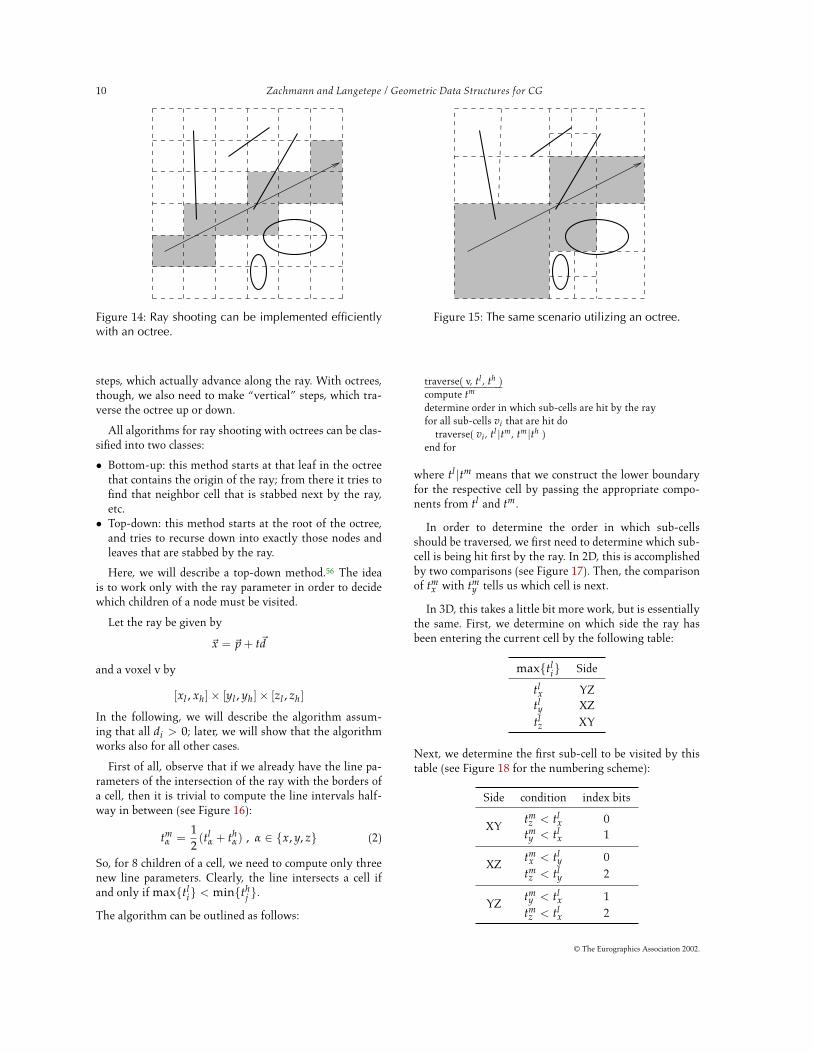
A simple idea to avoid checking the ray against all ob-jects is to partition the universe into a regular grid (seeFigure 14). With each cell we store a list of objects that oc-cupy that cell (at least partially). Then, we just walk alongthe ray from cell to cell, and check the ray against all thoseobjects that are stored with that cell.
In this scheme (and others), we need a technique calledmailboxes that prevents us from checking the ray twiceagainst the same object:27 every ray gets a unique ID (wejust increment a global variable holding that ID wheneverwe start with a new ray); during traversal, we store theray’s ID with the object whenever we have performed anintersection test with it. But before doing an intersectiontest with an object, we look into its mailbox whether or notthe current ray’s ID is already there; if so, then we knowthat we have already performed the intersection test in anearlier cell.
In the following, we will present two methods whichboth utilize octrees to further reduce the number of objectsconsidered.
2.5.1 3D Octree
A canonical way to improve any grid-based method is toconstruct an octree (see Figure 15). Here, the octree leavesstore lists of objects (or, rather, pointers to objects). Sincewe are dealing now with polygons and other graphical ob-jects, the leaf rule for the octree construction process mustbe changed slightly:
1. maximum depth reached; or,2. only one polygon/object occupies the cell.
We can try to better approximate the geometry of thescene by changing the rule to stop only when there areno objects in the cell (or the maximum depth is reached).
How do we traverse an octree along a given ray? Likein the case of a grid, we have to make “horizontal”
© The Eurographics Association 2002.
10 Zachmann and Langetepe / Geometric Data Structures for CG
Figure 14: Ray shooting can be implemented efficientlywith an octree.
Figure 15: The same scenario utilizing an octree.
steps, which actually advance along the ray. With octrees,though, we also need to make “vertical” steps, which tra-verse the octree up or down.
All algorithms for ray shooting with octrees can be clas-sified into two classes:
• Bottom-up: this method starts at that leaf in the octreethat contains the origin of the ray; from there it tries tofind that neighbor cell that is stabbed next by the ray,etc.
• Top-down: this method starts at the root of the octree,and tries to recurse down into exactly those nodes andleaves that are stabbed by the ray.
Here, we will describe a top-down method.56 The ideais to work only with the ray parameter in order to decidewhich children of a node must be visited.
Let the ray be given by
~x = ~p + t~d
and a voxel v by
[xl , xh]× [yl , yh]× [zl , zh]
In the following, we will describe the algorithm assum-ing that all di > 0; later, we will show that the algorithmworks also for all other cases.
First of all, observe that if we already have the line pa-rameters of the intersection of the ray with the borders ofa cell, then it is trivial to compute the line intervals half-way in between (see Figure 16):
tmα =
12(tl
α + thα) , α ∈ x, y, z (2)
So, for 8 children of a cell, we need to compute only threenew line parameters. Clearly, the line intersects a cell ifand only if maxtl
i < minthj .
The algorithm can be outlined as follows:
traverse( v, tl , th )compute tm
determine order in which sub-cells are hit by the rayfor all sub-cells vi that are hit do
traverse( vi , tl |tm, tm |th )end for
where tl |tm means that we construct the lower boundaryfor the respective cell by passing the appropriate compo-nents from tl and tm.
In order to determine the order in which sub-cellsshould be traversed, we first need to determine which sub-cell is being hit first by the ray. In 2D, this is accomplishedby two comparisons (see Figure 17). Then, the comparisonof tm
x with tmy tells us which cell is next.
In 3D, this takes a little bit more work, but is essentiallythe same. First, we determine on which side the ray hasbeen entering the current cell by the following table:
maxtli Side
tlx YZ
tly XZ
tlz XY
Next, we determine the first sub-cell to be visited by thistable (see Figure 18 for the numbering scheme):
Side condition index bits
XYtmz < tl
x 0tmy < tl
x 1
XZtmx < tl
y 0tmz < tl
y 2
YZtmy < tl
x 1tmz < tl
x 2
© The Eurographics Association 2002.

Zachmann and Langetepe / Geometric Data Structures for CG 11
thx
tlx
tly
tmx
tmy
thy
tmy > tl
x
tmy < tl
x
Figure 16: Line parameters are trivial to compute for chil-dren of a node.
Figure 17: The sub-cell that must be traversed first canbe found by simple comparisons. Here, only the casetlx > tl
y is depicted.
The first column is the entering side determined in the firststep. The third column yields the index of the first sub-cellto be visited: start with an index of zero; if one or both ofthe conditions of the second column hold, then the corre-sponding bit in the index as indicated by the third columnshould be set. Finally, we can traverse all sub-cells accord-ing to the following table:
current exit sidesub-cell YZ XZ XY
0 4 2 11 5 3 ex2 6 ex 33 7 ex ex4 ex 6 55 ex 7 ex6 ex ex 77 ex ex ex
where “exit side” means the exit side of the ray for thecurrent sub-cell.
If the ray direction contains a negative component(s),then we just have to mirror all tables along the respec-tive axis (axes) conceptually. This can be implemented ef-ficiently by an XOR operation.
2.5.2 5D Octree
In the previous, simple algorithm, we still walk along aray every time we shoot it into the scene. However, raysare essentially static objects, just like the geometry of thescene! This is the basic observation behind the followingalgorithm.1, 4 Again, it makes use of octrees to adaptivelydecompose the problem.
The underlying technique is a discretization of rays,which are 5-dimensional objects. Consider a cube enclos-ing the unit sphere of all directions. We can identify anyray’s direction with a point on that cube, hence it is calleddirection cube (see Figure 19). The nice thing about it
0 4
6
3 7
5
2
x
y
z
Figure 18: Sub-cells are numbered according to thisscheme.
is that we can now perform any hierarchical partitioningscheme that works in the plane, such as an octree: we justapply the scheme individually on each side.
Using the direction cube, we can establish a one-to-onemapping between direction vectors and points on all 6 sidesof the cube, i.e.,
S2 ↔ [−1, +1]2 × +x,−x, +y,−y, +z,−zWe will denote the coordinates on the cube’s side by u andv.
Within a given universe B = [0, 1]3 (we assume it is abox), we can represent all possibly occurring rays by pointsin
R = B× [−1, +1]2 × +x,−x, +y,−y, +z,−z (3)
which can be implemented conveniently by 6 copies of 5-dimensional boxes.
Returning to our goal, we now build six 5-dimensionaloctrees as follows. Associate (conceptually) all objects withthe root. Partition a node in the octree, if
1. there are too many objects associated with it; and2. the node’s cell is too large.
© The Eurographics Association 2002.

12 Zachmann and Langetepe / Geometric Data Structures for CG
uv
u
v
~d
=+
Figure 19: With the direction cube, we can discretize di-rections, and organize them with any hierarchical parti-tioning scheme.
Figure 20: A uv interval on the direction cube plus a xyzinterval in 3-space yield a beam.
If a node is partitioned, we must also partition its set ofobjects and assign each subset to one of the children.
Observe that each node in the 5D octree defines a beamin 3-space: the xyz-interval of the first three coordinatesof the cell define a box in 3-space, and the remaining twouv-intervals define a cone in 3-space. Together (more pre-cisely, their Minkowski sum) they define a beam in 3-spacethat starts at the cell’s box and extends in the general di-rection of the cone (see Figure 20).
Since we have now defined what a 5D cell of the octreerepresents, it is almost trivial to define how objects are as-signed to sub-cells: we just compare the bounding volumeof each object against the sub-cells 3D beam. Note thatan object can be assigned to several sub-cells (just like inregular 3D octrees). The test whether or not an object in-tersects a beam could be simplified further by enclosing abeam with a cone, and then checking the objects boundingsphere against that cone. This just increases the number offalse positives a little bit.
Having computed the six 5D octrees for a given scene,ray tracing through that octree is almost trivial: map theray onto a 5D point via the direction cube; start with theroot of that octree which is associated to the side of thedirection cube onto which the ray was mapped; find theleaf in that octree that contains the 5D point (i.e., the ray);check the ray against all objects associated with that leaf.
By locating a leaf in one of the six 5D octrees, we havediscarded all objects that do not lie in the general directionof the ray. But we can optimize the algorithm even further.
First of all, we sort all objects associated with a leaf alongthe dominant axis of the beam by their minimum (seeFigure 21). If the minimum coordinate of an object alongthe dominant axis is greater than the current intersectionpoint, then we can stop — all other possible intersectionpoints are farther away.
Second, we can utilize ray coherence as follows. Wemaintain a cache for each level in the ray tree that stores
the leaves of the 5D octrees that were visited last time.When following a new ray, we first look into the octreeleaf in the cache whether it is contained therein, before westart searching for it from the root.
Another trick (that works with other ray accelerationschemes as well) is to exploit the fact that we do not needto know the first occluder between a point on a surface anda light source. Any occluder suffices to assert that the pointis in shadow. So we also keep a cache with each light sourcewhich stores that object (or a small set) which has been anoccluder last time.
Finally, we would like to mention a memory optimiza-tion technique for 5D octrees, because they can occupy alot of memory. It is based on the observation that within abeam defined by a leaf of the octree the objects at the back(almost) never intersect with a ray emanating from thatcell (see Figure 22). So we store objects with a cell only ifthey are within a certain distance. Should a ray not hit anyobject, then we start a new intersection query with anotherray that has the same direction and a starting point just be-hind that maximum distance. Obviously, we have to makea trade-off between space and speed here, but when cho-sen properly, the cut-off distance should not reduce per-formance too much while still saving a significant amountof memory.
3 BSP TreesBSP trees (short for binary space partitioning trees) canbe viewed as a generalization of k-d trees. like k-d trees,BSP trees are binary trees, but now the orientation andposition of a splitting plane can be chosen arbitrarily. Toget a feeling for a BSP tree, Figure 23 shows an examplefor a set of objects.
The definition of a BSP (short for BSP tree) is fairlystraight-forward. Here, we will present a recursive defi-nition. Let h denote a plane in Rd, h+ and h− denote thepositive and negative half-space, resp.
© The Eurographics Association 2002.

Zachmann and Langetepe / Geometric Data Structures for CG 13
1 2 3 4
Figure 21: By sorting objects with in each 5D leaf, wecan often stop checking ray intersection quite early.
Figure 22: By truncating the beam (or rather, the list ofobjects) we can save a lot of memory usage of a 5Doctree, while reducing performance only insignificantly.
Definition 1 (BSP tree)Let S be a set of objects (points, polygons, groups of poly-gons, or other spatial objects), and let S(ν) denote the setof objects associated with a node ν. Then the BSP T(S) isdefined by
1. If |S| ≤ 1, then T is a leaf ν which stores S(ν) := S.2. If |S| > 1, then the root of T is a node ν; ν stores a
plane hν and a set S(ν) := x ∈ S|x ⊆ hν (this isthe set of objects that lie completely inside hν; in 3D,these can only be polygons, edges, or points). ν also hastwo children T− and T+; T− is the BSP for the set ofobjects S− := x ∩ h−ν |x ∈ S, and T+ is the BSP forthe set of objects S+ := x ∩ h+
ν |x ∈ S.
This can readily be turned into a general algorithm forconstructing BSPs. Note that a splitting step (i.e., the con-struction of an inner node) requires us to split each ob-ject into two disjoint fragments if it straddles the splittingplane of that node. In some applications though (such asray shooting), this is not really necessary; instead, we canjust put those objects into both subsets.
Note that with each node of the BSP a convex cell isassociated (which is possibly unbounded): the “cell” asso-ciated with the root is the whole space, which is convex;splitting a convex region into two parts yields two con-vex regions. In Figure 23, the convex region of one of theleaves has been highlighted as an example.
With BSPs, we have much more freedom to place thesplitting planes than with k-d trees. However, this alsomakes that decision much harder (as almost always in life).If our input is a set of polygons, then a very common ap-proach is to choose one of the polygons from the input set
h3
h4
h2
h1
h4
h2
h1
h3
Figure 23: An example BSP tree for a set of objects.
Figure 24: Left: an auto-partition. Right: an exampleconfiguration of which any auto-partition must havequadratic size.
and use this as the splitting plane. This is called an auto-partition (see Figure 24).
While an auto-partition can have Ω(n2) fragments, it ispossible to show the following in 2D.13, 53
Lemma 1Given a set S of n line segments in the plane, the ex-pected number of fragments in an auto-partition T(S) isin O(n log n); it can be constructed in time O(n2 log n).
In higher dimensions, it is not possible to show a similar
© The Eurographics Association 2002.

14 Zachmann and Langetepe / Geometric Data Structures for CG
nearpolygons
farpolygons
Figure 25: BSP trees are an efficient data structure encod-ing visibility order of a set of polygons.
result. In fact, one can construct sets of polygons such thatany BSP tree (not just auto-partitions) must have Ω(n2)many fragments (see Figure 24 for a “bad” example forauto-partitions).
However, all of these examples producing quadraticBSPs violate the principle of locality : polygons are smallcompared to the extent of the whole set. In practice,no BSPs have been observed that exhibit the worst-casequadratic behavior.49
3.1 Rendering Without a Z-Buffer
BSP trees were introduced to computer graphics byFuchs et al.25 At the time, hidden-surface removal was stilla major obstacle towards interactive computer graphics,because a z-buffer was just too costly in terms of mem-ory.
In this section, we will describe how to solve this prob-lem, not so much because the application itself is relevanttoday, but because it nicely exhibits one of the fundamen-tal “features” of BSP trees: they enable efficient enumer-ation of all polygons in visibility order from any point inany direction. (Actually, the first version of Doom used ex-actly this algorithm to achieve its fantastic frame rate (atthe time) on PCs even without any graphics accelerator.)
A simple algorithm to render a set of polygons with cor-rect hidden-surface removal, and without a z-buffer, is thepainter’s algorithm : render the scene from back to front asseen from the current viewpoint. Front polygons will justoverwrite the contents of the frame buffer, thus effectivelyhiding the polygons in the back. There are polygon config-urations where this kind of sorting is not always possible,but we will deal with that later.
How can we efficiently obtain such a visibility orderof all polygons? Using BSP trees, this is almost trivial:starting from the root, first traverse the branch that doesnot contain the viewpoint, then render the polygon stored
2 3
1
6
in out
out5 4
7in out out
in out
3
out
out
out
out
out
inin
6
7
42
1in
5
Figure 26: Each leaf cell of BSP representation of an ob-ject is completely inside or completely outside.
with the node, then traverse the other branch containingthe viewpoint (see Figure 25).
For sake of completeness, we would like to mention afew strategies to optimize this algorithm. First of all, weshould make use of the viewing direction by skipping BSPbranches that lie completely behind the viewpoint.
Furthermore, we can perform back-face culling as usual(which does not cause any extra costs). We can also per-form view-frustum culling by testing all vertices of thefrustum against the plane of a BSP node.
Another problem with the simple algorithm is that apixel is potentially written to many times (this is exactlythe pixel complexity), although only the last write “sur-vives”. To remedy this, we must traverse the BSP fromfront to back. But in order to actually save work, we alsoneed to maintain a 2D BSP for the screen that allows usto quickly discard those parts of a polygon that fall onto ascreen area that is already occupied. In that 2D screen BSP,we mark all cells either “free” or “occupied”. Initially, itconsists only of a “free” root node. When a new polygonis to be rendered, it is first run through the screen BSP,splitting it into smaller and smaller convex parts until itreaches the leaves. If a part reaches a leaf that is alreadyoccupied, nothing happens; if it reaches a free leaf, then itis inserted beneath that leaf, and this part is drawn on thescreen.
3.2 Representing Objects with BSPs
BSPs offer a nice way to represent volumetric polygonalobjects, which are objects consisting of polygons that areclosed, i.e., they have an “inside” and an “outside”. Sucha BSP representation of an object is just like an ordinaryBSP for the set of polygons (we can, for instance, buildan auto-partition), except that here we stop the construc-tion process (see Definition 1) only when the set is empty.These leaves represent homogeneous convex cells of thespace partition, i.e., they are completely “in” our “out”.
© The Eurographics Association 2002.

Zachmann and Langetepe / Geometric Data Structures for CG 15
A B
∩∪ \ ª
Figure 27: Using BSPs, we can efficiently compute theseboolean operations on solids.
TH
Figure 28: The fundamental step of the construction isthis simple operation, which merges a BSP and a plane.
Figure 26 shows an example for such a BSP represen-tation. In this section, we will follow the convention thatnormals point to the “outside”, and that the right childof a BSP node lies in the positive half-space and the leftchild in the negative half-space. So, in a real implemen-tation that adheres to these conventions, we can still stopthe construction when only one polygon is left, because weknow that the left child of such a pseudo-leaf will be “in”and the right one will be “out”.
Given such a representation, it is very easy and efficient,for instance, to determine whether or not a given a pointis inside an object. In the next section, we will describe analgorithm for solving a slightly more difficult problem.
3.3 Boolean Operations
In solid modeling, a very frequent task is to computethe intersection or union of a pair of objects. More gen-erally, given two objects A and B, we want to computeC := A op B, where op ∈ ∪,∩, \,ª (see Figure 27).This can be computed efficiently using the BSP represen-tation of objects.48, 49 Furthermore, the algorithm is almostthe same for all of these operations: only the elementarystep that processes two leaves of the BSPs is different.
We will present the algorithm for boolean operationsbottom-up in three steps. The first step is a sub-procedurefor computing the following simple operation: given a BSP
R(T)
"leaf"
HT
pT
"anti-parallel on"
pT
"pos./pos."
HTP HT
"mixed"
HHH
Figure 29: The main building block of the algorithm con-sists of these four cases (plus analogous ones).
+ →→
Figure 30: Computation of boolean operations is basedon a general merge operation.
T and a plane H, construct a new BSP T whose root is H,such that T− , T ∩ H− , T+ , T ∩ H+ (see Figure 28).This basically splits a BSP tree by a plane and then putsthat plane at the root of the two halves. Since we will notneed the new tree T explicitly, we will describe only thesplitting procedure (which is the bulk of the work any-way).
First, we need to define some nomenclature:
T− , T+ = left and right child of T, resp.
R(T) = region of the cell of node T (which is convex)
T⊕ , Tª =portion of T on the positive/negativeside of H, resp.
Finally, we would like to define a node T by the tuple(HT , pT , T− , T+), where H is the splitting plane, p is thepolygon associated with T (with p ⊂ H).
The pseudo-code below is organized into 8 cases (seeFigure 29):
split-tree( T, H, P ) → (Tª , T⊕)P = H ∩ R(T)case T is a leaf :
return (Tª , T⊕) := (T, T)case “anti-parallel” and “on” :
return (Tª , T⊕) := (T+ , T−)case “parallel” and “on” :
. . .case “pos./pos.” :
(T+ª , T+⊕) := split-tree(T+ , H)Tª := (HT , pT , T− , T+ª)T⊕ := T+⊕
case “pos./neg.” :. . .
case “neg./pos.” :. . .
case “neg./neg.” :. . .
case “mixed” :(T+ª , T+⊕) := split-tree(T+ , H, P ∩ R(T+))
© The Eurographics Association 2002.

16 Zachmann and Langetepe / Geometric Data Structures for CG
split merge merge
combine
Figure 31: A graphical depiction of the merge step in the algorithm for boolean operations on objects represented byBSP trees.
(T−ª , T−⊕) := split-tree(T− , H, P ∩ R(T−))Tª := (HT , pT ∩ H− , T−ª , T+ª)T⊕ := (HT , pT ∩ H+ , T−⊕ , T+⊕)return (Tª , T⊕)
end case
This might look a little bit confusing at first sight, but it isreally pretty simple. A few notes might be in order.
The polygon P is only needed in order to find the caseapplying at each recursion. Computing P ∩ R(T+) mightseem very expensive. However, it can be computed quiteefficiently by computing P∩H+
T , which basically amountsto finding the two edges that intersect with HT . Please seeChin12 for more details on how to detect the correct case.
It seems surprising at first sight that function split-
tree does almost no work — it just traverses the BSP tree,classifies the case found at each recursion, and computesp ∩ H+ and p ∩ H−.
The previous algorithm is already the main buildingblock of the overall boolean operation algorithm. The nextstep towards that end is an algorithm that performs a so-called merge operation on two BSP trees T1 and T2. LetCi denote the set of elementary cells of a BSP, i.e., all re-gions R(Lj) of tree Ti where Lj are all the leaves. Thenthe merge of T1 , T2 yields a new BSP tree T3 such thatC3 = c1 ∩ c2|c1 ∈ C1 , c2 ∈ C2 , c1 ∩ c2 6= ∅ (see Fig-ure 30).
The merge operation consists of two cases. The first, al-most trivial, case occurs when one of the two operands isa leaf: then at least one of the two regions is homogenous,i.e., completely inside or outside. In the other case, bothtrees are inhomogenous over the same region of space:then, we just split one of the two with the splitting planefrom the root of the other, and we obtain two pairs of BPSs,that are smaller, and still cover the same regions in space;those two pairs can be merged recursively (see Figure 31).
The following pseudo-code describes this recursive proce-dure more formally:
merge( T1, T2 ) → T3if T1 or T2 is a leaf then
perform the cell-op as required by the boolean operation tobe constructed (see below)
else(Tª2 , T⊕2 ) := split-tree(T2 , H1 , . . .)T−3 := merge(T−1 , Tª2 )T+
3 := merge(T+1 , T⊕2 )
T3 := (H1 , T−3 , T+3 )
end if
The function cell-op is the only place where the se-mantic of the general merge operation is specialized. Whenwe have reached that point, then we know that one of thetwo cells is homogeneous, so we can just replace it by theother node’s sub-tree suitably modified according to theboolean operation. The following table lists the details ofthis function (assuming that T1 is the leaf):
Operation T1 Result
∪ in T1out T2
∩ in T2out T1
\ in Tc2
out T1
ª in Tc2
out T2
Furthermore, we would like to point out that the mergefunction is symmetric: it does not matter whether we par-tition T2 with H1 or, the other way round, T1 with H2 —the result will be the same.
© The Eurographics Association 2002.

Zachmann and Langetepe / Geometric Data Structures for CG 17
4 Bounding Volume HierarchiesLike the previous hierarchical data structures, bound-ing volume hierarchies (BVHs) are mostly used to pre-vent performing an operation exhaustively on all objects.Like with previously discussed hierarchical data struc-tures, one can improve a huge range of applications andqueries using BVHs, such as ray shooting, point locationqueries, nearest-neighbor search, view frustum and occlu-sion culling, geographical data bases, and collision detec-tion (the latter will be discussed in more detail below).
Often times, bounding volume (BV) hierarchies are de-scribed as the opposite of spatial partitioning schemes,such as quadtrees or BSP trees: instead of partitioningspace, the idea is to partition the set of objects recursivelyuntil some leaf criterion is met. (However, we will argueat the end that BV hierarchies are just at the other endof a whole spectrum of hierarchical data structures.) Here,objects can be anything from points to complete graphi-cal objects. With BV hierarchies, almost all queries, whichcan be implemented with space partitioning schemes, canalso be answered, too. Example queries and operations areray shooting, frustum culling, occlusion culling, point lo-cation, nearest neighbor, collision detection.
Definition 2 (BV hierarchy)Let O = o1 , . . . , on be a set of elementary objects. Abounding volume hierarchy for O, BVH(O), is defined by
1. If |O| = e, then BVH(O) := a leaf node that stores Oand a BV of O;
2. If |O| > e, then BVH(O) := a node ν with n(ν) chil-dren ν1 , . . . , νn, where each child νi is a BV hierarchyBVH(Oi) over a subset Oi ⊂ O, such that
⋃Oi = O.
In addition, ν stores a BV of O.
The definition mentions two parameters. The thresholde is often set to 1, but depending on the application, the op-timal e can be much larger. Just like sorting, when the setof objects is small, it is often cheaper to perform the oper-ation on all of them, because recursive algorithms alwaysincur some overhead.
Another parameter in the definition is the arity. Mostly,BV hierarchies are constructed as binary trees, but again,the optimum can be larger. And what is more, as the defi-nition suggests, the out-degree of nodes in a BV hierarchydoes not necessarily have to be constant, although this of-ten simplifies implementations considerably.
Effectively, these two parameters, e and n(ν), controlthe balance between linear, exhaustive search/operation,and a maximally recursive algorithm.
There are more design choices possible according to thedefinition. For inner nodes, it only requires that
⋃Oi = O;
this means, that the same object o ∈ O could be associatedwith several children. Depending on the application, the
convex hull
AABB sphere DOP OBB spherical shell
prism cylinder intersectionof other BVs
Figure 32: Some of the most commonly used BVs, andsome less often used ones.
type of BVs, and the construction process, this may not al-ways be avoidable. But if possible, you should always splitthe set of objects into disjoint subsets.
Finally, there is, at least, one more design choice: thetype of BV used at each node. Again, this does not nec-essarily mean that each node uses the same type of BV.Figure 32 shows a number of the most commonly usedBVs. The difference between OBBs4 and AABBs is thatOBBs can be oriented arbitrarily (hence “oriented bound-ing boxes”). DOPs67, 39, 37 are a generalization of AABBs:basically, they are the intersection of k slabs. Prisms andcylinders have been proposed by Barequet et al.7 andWeghorst et al.63, but they seem to be too expensive com-putationally. A spherical shell is the intersection of a shelland a cone (the cone’s apex coincides with the sphere’scenter), and a shell is the space between two concentricspheres. Finally, one can always take the intersection oftwo or more different types of BVs.36
There are three characteristic properties of BVs:
• tightness,• memory usage,• number of operations needed to test the query object
against a BV.
Often, one has to make a trade-off between these proper-ties: generally, the type of BV that offers better tightnessalso requires more operations per query and more mem-ory.
Regarding the tightness, one can establish a theoreticaladvantage of OBBs. But first, we need to define tightness.29
Definition 3 (Tightness by Hausdorff distance)Let B be a BV, G some geometry bounded by B, i.e., g ⊂ B.Let
h(B, G) = maxb∈B
ming∈G
d(b, g)
be the directed Hausdorff distance, i.e., the maximum dis-tance of B to the nearest point in G. (Here, d is any metric,
© The Eurographics Association 2002.

18 Zachmann and Langetepe / Geometric Data Structures for CG
diam(G)
B
G
h(B, G)
d
h
h′
φ Œ/2
hd
Figure 33: One way to define tight-ness is via the directed Hausdorffdistance.
Figure 34: The tightness of anAABB remains more or less con-stant throughout the levels of aAABB hierarchy for surfaces ofsmall curvature.
Figure 35: The tightness of an OBBdecreases for deeper levels in aOBB hierarchy for small curvaturesurfaces.
very often just the Euclidean distance.) Let
diam(G) = maxg, f∈G
d(g, f )
be the diameter of G.
Then we can define tightness
τ :=h(B, G)
diam(G).
See Figure 33 for an illustration.
Since the Hausdorff distance is very sensitive to out-liers, one could also think of other definitions such as thefollowing one:
Definition 4 (Tightness by volume)Let C(ν) b the set of children of a node ν of the BV hi-erarchy. Let Vol(ν) be the volume of the BV stored withν.
Then, we can define the tightness as
τ :=Vol(ν)
∑ν′∈C(ν) Vol(ν′).
Alternatively, we can define it as
τ :=Vol(ν)
∑ν′∈L(ν) Vol(ν′),
where L(ν) is the set of leaves beneath ν.
Getting back to the tightness definition based on theHausdorff distance, we observe a fundamental differencebetween AABBs and OBBs:29
• The tightness of AABBs depends on the orientation ofthe enclosed geometry. What is worse is that the tight-ness of the children of an AABB enclosing a surface ofsmall curvature is almost the same as that of the father.The worst case is depicted in Figure 34. The tightness ofthe father is τ = h/d, while the tightness of a child is
τ′ = h′d/2 = h/2
d/2 = τ.
• The tightness of OBBs does not depend on the orienta-tion of the enclosed geometry. Instead, it depends on itscurvature, and it decreases approximately linearly withthe depth in the hierarchy.Figure 35 depicts the situation for a sphere. The Haus-dorff distance from an OBB to an enclosed spherical arcis h = r(1 − cos φ), while the diameter of the arc isd = 2r sin φ. Thus, the tightness for an OBB bound-
ing a spherical arc of degree φ is τ = 1−cos φ2 sin φ , which
approaches 0 linearly as φ → 0.
This makes OBBs seem much more attractive thanAABBs. The price of the much improved tightness is, ofcourse, the higher computational effort needed for mostqueries per node when traversing an OBB tree with aquery.
4.1 Construction of BV Hierarchies
Essentially, there are 3 strategies to build BV trees:
• bottom-up,• top-down,• insertion
From a theoretical point of view, one could pursue a simpletop-down strategy, which just splits the set of objects into
© The Eurographics Association 2002.

Zachmann and Langetepe / Geometric Data Structures for CG 19
two equally sized parts, where the objects are assigned ran-domly to either subset. Asymptotically, this yields usuallythe same query time as any other strategy. However, inpractice, the query times offered by such a BV hierarchyare by a large factor worse.
During construction of a BV hierarchy, it is convenientto forget about the graphical objects or primitives, and in-stead deal with their BVs and consider those as the atoms.Sometimes, another simplification is to just approximateeach object by its center (baryenter or bounding box cen-ter), and then deal only with sets of points during the con-struction. Of course, when the BVs are finally computedfor the nodes, then the true extents of the objects must beconsidered.
In the following we will describe algorithms for eachconstruction strategy.
4.1.1 Bottom-up
In this class, we will actually describe two algorithms.
Let B be the set of BVs on the top-most level of theBV hierarchy that has been constructed so far.57 For eachbi ∈ B find the nearest neighbor b′i ∈ B; let di be thedistance between bi and b′i . Sort B with respect to di. Then,combine the first k nodes in B under a common father; dothe same with the next k elements from B, etc. This yieldsa new set B′, and the process is repeated.
Note that this strategy does not necessarily produce BVswith a small “dead space”: in Figure 36, the strategy wouldchoose to combine the left pair (distance = 0), while choos-ing the right pair would result in much less dead space.
The second strategy is less greedy in that it computes atiling for each level. We will describe it first in 2D.42 Again,let B be the set of BVs on the top-most level so far con-structed, with |B| = n. The algorithm first computes thecenter ci for each bi ∈ B. Then, it sorts B along the x-axiswith respect to ci
x. Now, the set B is split into√
n/k vertical“slices” (again with respect to ci
x). Now, each slice is sortedaccording to ci
y and subsequently split into√
n/k “tiles”,so that we end up with k tiles (see Figure 37). Finally, allnodes in a tile are combined under one common father, itsBV is combined, and the process repeats with a new set B′.
In Rd it works quite similarly: we just split each slicerepeatedly by d
√n/k along all coordinate axes.
4.1.2 Insertion
This construction scheme starts with an empty tree. Let Bbe the set of elementary BVs. The following pseudo-codedescribes the general procedure:
1: while |B| > 0 do2: choose next b ∈ B3: ν := root
ν
ν′
θν′
θν
Figure 38: The probability of a ray hitting a child box canbe extimated by the surface area.
4: while ν 6= leaf do5: choose child ν′,
so that insertion of b into ν′ causes minimal increasein the costs of the total tree
6: ν := ν′
7: end while8: end while
All insertion algorithms only vary step 2 and/or 5. Step 2is important because a “bad” choice in the beginning canprobably never be made right afterwards. Step 5 dependson the type of query that is to be performed on the BVtree. See below for a few criteria.
Usually, algorithms in this class have complexityO(n log n).
4.1.3 Top-down
This scheme is the most popular one. It seems to producevery good hierarchies while still being very efficient, andusually it can be implemented easily.
The general idea is to start with the complete set of el-ementary BVs, split that into k parts, and create a BV treefor each part recursively. The splitting is guided by someheuristic or criterion that (hopefully) produces good hier-archies.
4.1.4 Criteria
In the literature, there is a vast number of criteria forguiding the splitting, insertion, or merging, during BVtree construction. (Often, the authors endow the thus con-structed BV hierarchy with a new name, even though theBVs utilized are well known.) Obviously, the criterion de-pends on the application for which the BV tree is to beused. In the following, we will present a few of these cri-teria.
For ray tracing, if we can estimate the probability that aray will hit a child box when it has hit the father box, thenwe know how likely it is, that we need to visit the childnode when we have visited the father node. Let us assumethat all rays emanate from the same origin (see Figure 38).
© The Eurographics Association 2002.

20 Zachmann and Langetepe / Geometric Data Structures for CG
Figure 36: A simple greedy strategy can produce much“dead space”.
Figure 37: A less greedy strategy combines BVs by com-puting a “tiling”.
Then, we can observe that the probability that a ray s hitsa child box ν′ under the condition that it has hit the fatherbox ν is
P(s hits ν′|s hits ν) =θν′
θν≈ Area(ν′)
Area(ν)(4)
where Area denotes the surface area of the BV, and θ de-notes the solid angle subtended by the BV. This is becausefor a convex object, the solid angle subtended by it, whenseen from large distances, is approximately proportional toits surface area.28 So, a simple strategy is to just minimizethe surface area of the BVs of the children that are pro-duced by a split. (For the insertion scheme, the strategy isto choose that child node whose area is increased least.28)
A more elaborate criterion tries to establish a cost func-tion for a split and minimize that. For ray tracing, this costfunction can be approximated by
C(ν1 , ν2) =Area(ν1)Area(ν)
C(ν1) +Area(ν2)Area(ν)
C(ν2) (5)
where ν1 , ν2 are the children of ν. The optimal split B =B1 ∪ B2 minimizes this cost function:
C(B1 , B2) = minB′∈P(B)
C(B′ , B \ B′)
where B1 , B2 are the subsets of elementary BVs (or ob-jects) assigned to the children. Here, we have assumed abinary tree, but this can be extended to other arities anal-ogously.
Of course, such a minimization is too expensive inpractice, in particular, because of the recursive defini-tion of the cost function. So, Fussell and Subramanian26,Müller et al.47, and Beckmann et al.8 have proposed thefollowing approximation algorithm:
for α = x, y, z dosort B along axis α with respect to the BV centersfind
kα = minj=0...n
Area(b1 , . . . , bj)
Area(B)j +
Area(bj+1 , . . . , bn)Area(B)
(n− j)
end forchoose the best kα
where Area(b1 , . . . , bj) denotes the surface area of the BVenclosing b1 , . . . , bj.
If the query is a point location query (e.g., is a givenpoint inside or outside the object), then the volume in-stead of the surface area should be used. This is becausethe probability that a point is contained in a child BV, un-der the condition that it is contained in the father BV, isproportional to the ratio of the two volumes.
For range queries, and for collision detection, the vol-ume seems to be a good probability estimation, too.
A quite different splitting algorithm does not (ex-plicitely) try to estimate any probabilities. It just approx-imates each elementary BV/object by its center point. Itthen proceeds as follows. For a given set B of such points,compute its principal components (the Eigenvectors of thecovariance matrix); choose the largest of them (i.e., theone exhibiting the largest variance); place a plane orthog-onal to that principal axis and through the barycenter ofall points in B; finally, split B into two subsets accordingto the side on which the point lies. (This description is aslightly modified version of Gottschalk et al.29.) Alterna-tively, one can place the splitting plane through the median
© The Eurographics Association 2002.

Zachmann and Langetepe / Geometric Data Structures for CG 21
B2
B1
B
A
A1
A2
Figure 40: Hierarchical collision detection can discardmany pairs of polygons with one BV check. Here, allpairs of polygons in A1 and B2 can be discarded.
of all points, instead of the barycenter. This would lead tobalanced trees, but not necessarily better ones.
4.2 Collision Detection
Fast and exact collision detection of polygonal objects un-dergoing rigid motions is at the core of many simulationalgorithms in computer graphics. In particular, all kinds ofhighly interactive applications such as virtual prototypingneed exact collision detection at interactive speed for verycomplex, arbitrary “polygon soups”. It is a fundamentalproblem of dynamic simulation of rigid bodies, simulationof natural interaction with objects, and haptic rendering.
Bounding volume trees seem to be a very efficientdata structure to tackle the problem of collision detec-tion for rigid bodies. All kinds of different types of BVshave been explored in the past: sphere trees32, 52, OBBtrees29, DOP trees39, 67, AABB trees66, 60, 40, and convex hullhierarchies21, to name but a few.
Given two hierarchical BV volume data structures fortwo objects A and B, almost all hierarchical collision de-tection algorithms implement the following general algo-rithm scheme:
traverse(A,B)if A and B do not overlap then
returnend ifif A and B are leaves then
return intersection of primitivesenclosed by A and B
elsefor all children A[i] and B[j] do
traverse(A[i],B[j])end for
end if
This algorithm quickly “zooms in” on pairs of close poly-gons. The characteristics of different hierarchical collisiondetection algorithms lie in the type of BV used, the overlaptest for a pair of nodes, and the algorithm for constructionof the BV trees.
The algorithm outlined above is essentially a simultane-ous traversal of two hierarchies, which induces a so-calledrecursion tree (see Figure 39). Each node in this tree de-notes a BV overlap test. Leaves in the recursion tree denotean intersection test of the enclosed primitives (polygons);whether or not a BV test is done at the leaves depends onhow expensive it is, compared to the intersection test ofprimitives.
During collision detection, the simultaneous traversalwill stop at some nodes in the recursion tree. Let us callthe set of nodes, of which some children are not visited(because their BVs do not overlap), the “bottom slice”through the recursion tree (see the dashed lines in Fig-ure 39).
One idea is to save this set for a given pair of objects43.When this pair is to be checked next time, we can startfrom this set, going either up or down. Hopefully, if theobjects have moved only a little relative to each other, thenumber of nodes that need to be added or removed fromthe bottom slice is small. This scheme is called incrementalhierarchical collision detection.
5 Voronoi DiagramsFor a given set of sites inside an area the Voronoi diagramis a partition of the area into regions of the same neighbor-ship. The Voronoi diagram and its dual have been used forsolving numerous problems in many fields of science.
We will concentrate on its application to geometricproblems in 2D and 3D. For an overview of the Voronoidiagram and its dual in computational geometry one mayconsult the surveys by Aurenhammer2, Bernal9, Fortune24
and Aurenhammer and Klein3. Additionally, chapters 5and 6 of Preparata and Shamos54 and chapter 13 ofEdelsbrunner19 could be consulted.
We start in Section 5.1 with the simple case of theVoronoi diagram and the Delaunay triangulation of npoints in the plane, under the Euclidean distance. Addi-tionally we mention some of the elementary structuralproperties that follow from the definitions.
In Section 5.2 different algorithmic schemes for com-puting the structures are mentioned. We present a sim-ple incremental construction approach which can easily begeneralized to 3D, see Section 5.3.1.
Apart from the Euclidean 3D case some other interest-ing generalizations are mentioned in Section 5.3.2.
© The Eurographics Association 2002.

22 Zachmann and Langetepe / Geometric Data Structures for CG
F7 G6 G7F6E4D4 D5 E5E F GD
CB
A
5 6 74
2 3
1
D7D6 G4 G5
A1
B2 B3 C2 C3
F4 F5E6 E7
Figure 39: The recursion tree is induced by the simultaneous traversal of two BV trees.
In Section 5.4 the relevance of the Voronoi diagram andthe Delaunay triangulation in 3D are shown.
Note, that we can only sketch many of the subjects here.For further details and further literature see one of the sur-veys mentioned above. The figures are taken from Auren-hammer and Klein.3
5.1 Definitions and Elementary Properties
5.1.1 Voronoi Diagram
Let S a set of n ≥ 3 point sites p, q, r, . . . in the plane.In the following we assume that the points are in generalposition, i.e., no four of them lie on the same circle and nothree of them on the same line.
For points p = (p1 , p2) and x = (x1 , x2) let d(p, x)denote their Euclidean distance. By pq we denote the linesegment from p to q. The closure of a set A will be denotedby A.
Definition 5For p, q ∈ S let
B(p, q) = x | d(p, x) = d(q, x)be the bisector of p and q. B(p, q) is the perpendicular linethrough the center of the line segment pq. It separates thehalfplane
D(p, q) = x | d(p, x) < d(q, x)containing p from the halfplane D(q, p) containing q. Wecall
VR(p, S) =⋂
q∈S,q 6=p
D(p, q)
the Voronoi region of p with respect to S. Finally, theVoronoi diagram of S is defined by
V(S) =⋃
p,q∈S,p 6=q
VR(p, S) ∩VR(q, S).
An illustration is given in Figure 41. It shows how theplane is decomposed by V(S) into Voronoi regions. Notethat it is convenient to imagine a simple closed curve Γaround the “interesting” part of the Voronoi diagram.
Γ
Figure 41: A Voronoi diagram of points in the Euclideanplane.
The common boundary of two Voronoi regions belongsto V(S) and is called a Voronoi edge, if it contains morethan one point. If the Voronoi edge e borders the regionsof p and q then e ⊂ B(p, q) holds. Endpoints of Voronoiedges are called Voronoi vertices; they belong to the com-mon boundary of three or more Voronoi regions.
There is an intuitive way of looking at the Voronoi di-agram. For any point x in the plane we can expand thecircle C(r) with center x and radius r by increasing r con-tinuously. We detect three cases depending on which eventoccurs first:
© The Eurographics Association 2002.

Zachmann and Langetepe / Geometric Data Structures for CG 23
• If C(r) hits one of the n sites, say p, then x ∈ VR(p, S).• If C(r) hits two sites p and q simultaneously x belongs
to the Voronoi edge of p and q.• If C(r) hits three sites p, q and r simultaneously x is the
Voronoi vertex of p, q and r.
We will enumerate some of the significant properties ofVoronoi diagrams.
1. Each Voronoi region VR(p, S) is the intersection of atmost n− 1 open halfplanes containing the site p. EveryVR(p, S) is open and convex. Different Voronoi regionsare disjoint.
2. A point p of S lies on the convex hull of S iff its Voronoiregion VR(p, S) is unbounded.
3. The Voronoi diagram V(S) has O(n) many edges andvertices. The average number of edges in the boundaryof a Voronoi region is less than 6.
The Voronoi diagram is a simple linear structure andprovides for a partition of the plane into cells of the sameneighborship. We omit the proofs and refer to the surveysmentioned in the beginning.
Note, that the Voronoi edges and vertices build a graph.Therefore the diagram normally is represented by a graphof linear size. For example the diagram can be representedby a doubly connected edge list DCEL, see de Berg et al.13,or with the help of an adjacency matrix.
5.1.2 Delaunay Triangulation
We consider the dual graph of the Voronoi diagram, theso called Delaunay triangulation. In general, a triangula-tion of S is a planar graph with vertex set S and straightline edges, which is maximal in the sense that no fur-ther straight line edge can be added without crossing otheredges. The triangulation of a point set S has not more thanO(|S|) triangles.
Definition 6The Delaunay triangulation DT(S) is the dual Graph ofthe Voronoi diagram. The edges of DT(S) are called De-launay edges.
Obviously, the Delaunay triangulation DT(S) is a trian-gulation of S, an example is shown in Figure 42.
We present two equivalent definitions of the Delaunaytriangulation. They are applied for the computation of thediagram and give also rise to generalization, for example ifthe dual of a Voronoi diagram is no longer well-defined.
1. Two points p, q of S give rise to a Delaunay edge iff acircle C exists that passes through p and q and does notcontain any other site of S in its interior or boundary.
2. Three points of S give rise to a Delaunay triangle ifftheir circumcircle does not contain a point of S in itsinterior.
DT(S)
V(S)w
p
s
vr
q
Figure 42: Voronoi diagram and Delaunay triangulation.
5.2 Computation
The construction of the Voronoi diagram has time com-plexity Θ(n log n). The lower bound Ω(n log n) can beachieved by the following reductions.
• A reduction to the convex hull problem is given byShamos.58
• A reduction to the ε-closeness problem is given by Djid-jev and Lingas16 and by Zhu and Mirzaian68.
The well-known computation paradigms
• Incremental construction,• Divide-and-Conquer and• Sweep
are convenient for the construction of the Voronoi diagramor the Delaunay triangulation, respectively. They can alsobe generalized to other metrics and sites other than points,for example line segments or polygonal chains. The resultof the algorithms is stored in a graph of linear size, seeabove.
All these approaches run in deterministic O(n log n).We explain a simple Incremental construction techniquewhich runs in O(n log n) expected time and computes theDelaunay triangulation. The presentation is adapted fromKlein and Aurenhammer.3 The technique can easily begeneralized to the three dimensional case as we will seein Section 5.3.1.
Simple incremental construction: The insertion pro-cess is described as follows: We construct DTi =DT(p1 , . . . , pi−1 , pi) by inserting the site pi intoDTi−1. We follow Guibas and Stolfi30 and construct DTiby exchanging edges, using Lawson’s41 original edge flip-ping procedure, until all edges invalidated by pi have beenremoved.
It is helpful to extend the notion of triangle to the un-bounded face of the Delaunay triangulation. If pq is anedge of the convex hull of S we call the supporting outerhalfplane H not containing S an infinite triangle withedge pq. Its circumcircle is H itself, the limit of all circlesthrough p and q whose center tend to infinity within H.
© The Eurographics Association 2002.

24 Zachmann and Langetepe / Geometric Data Structures for CG
As a consequence, each edge of a Delaunay triangulationis now adjacent to two triangles.
Those triangles of DTi−1 whose circumcircles containthe new site, pi, are said to be in conflict with pi. Accord-ing to the (equivalent) definition of the DTi, they will nolonger be Delaunay triangles.
Let qr be an edge of DTi−1, and let T(q, r, t) be the tri-angle adjacent to qr that lies on the other side of qr thanpi; see Figure 43. If its circumcircle C(q, r, t) contains pithen each circle through q, r contains at least one of pi , t.Consequently, qr cannot belong to DTi, due to the (equiv-alent) definition. Instead, pit will be a new Delaunay edge,because there exists a circle contained in C(q, r, t) that con-tains only pi and t in its interior or boundary. This processof replacing edge qr by pit is called an edge flip.
pi
q
t
r
C(pi,t)
C(q,r,t)
Figure 43: If triangle T(q, r, t) is in conflict with pi thenformer Delaunay edge qr must be replaced by pit.
The necessary edge flips can be carried out efficiently ifwe know the triangle T(q, s, r) of DTi−1 that contains pi,see fig. Figure 44. The line segments connecting pi to q, r,and s will be new Delaunay edges, by the same argumentfrom above. Next, we check if e. g. edge qr must be flipped.If so, the edges qt and tr are tested, and so on. We continueuntil no further edge currently forming a triangle with,but not containing pi, needs to be flipped, and obtain DTi.
Two task have to be considered:
1. Find the triangle of DTi−1 that is in conflict with pi.2. Perform all flips starting from this triangle.
It can be shown that the second task is bounded by thedegree of pi in the new triangulation. If the triangle ofDTi−1 containing pi is known, the structural work neededfor computing DTi from DTi−1 is proportional to the de-gree d of pi in DTi.
So we yield an obvious O(n2) time algorithm for con-structing the Delaunay triangulation of n points: we candetermine the triangle of DTi−1 containing pi within lin-ear time, by inspecting all candidates. Moreover, the degreeof pi is trivially bounded by n.
The last argument is too crude. There can be single ver-tices in DTi that do have a high degree, but their averagedegree is bounded by 6.
With a special implementation using a directed acyclicgraph (DAG), also called Delaunay tree due to Boissonnatand Teillaud10, we can detect the triangles of DTi−1 whichare in conflict with pi in O(log i) expected time.
Altogether we get the following result:
Theorem 7The Delaunay triangulation of a set of n points in the planecan be easily incrementally constructed incrementally inexpected time O(n log n), using expected linear space. Theaverage is taken over the different orders of inserting then sites.
5.3 Generalization of the Voronoi Diagram
5.3.1 Voronoi Diagram and Delaunay Triangulationin 3D
We will see that incremental construction is also appropri-ate for the 3D case. The following description was adaptedfrom Aurenhammer and Klein.3
Let S be a set of n point sites in 3D. The bisector of twosites p, q ∈ S is the perpendicular plane through the mid-point of the line segment pq. The region VR(p, S) of a sitep ∈ S is the intersection of halfspaces bounded by bisec-tors, and thus is a 3-dimensional convex polyhedron. Theboundary of VR(p, S) consists of facets (maximal subsetswithin the same bisector), of edges (maximal line segmentsin the boundary of facets), and of vertices (endpoints ofedges). The regions, facets, edges, and vertices of V(S) de-fine a cell complex in 3D.
This cell complex is face-to-face: if two regions have anon-empty intersection f , then f is a face (facet, edge, orvertex) of both regions. As an appropriate data structurefor storing a 3-dimensional cell complex we mention thefacet-edge structure in Dobkin and Laszlo.17
Complexity: The number of facets of VR(p, S) is atmost n− 1, at most one for each site q ∈ S \ p. Hence,by the Eulerian polyhedron formula, the number of edgesand vertices of VR(p, S) is O(n), too. This shows that thetotal number of components of the diagram V(S) in 3D isO(n2). In fact, there are configurations S that force eachpair of regions of V(S) to share a facet, thus achievingtheir maximum possible number of
(n2); see, e.g., Dewd-
ney and Vranch.15 This fact sometimes makes Voronoi dia-grams in 3D less useful compared to 2-space. On the otherhand, Dwyer18 showed that the expected size of V(S) ind-space is only O(n), provided S is drawn uniformly atrandom in the unit ball. This result indicates that high-dimensional Voronoi diagrams will be small in many prac-tical situations.
© The Eurographics Association 2002.

Zachmann and Langetepe / Geometric Data Structures for CG 25
(i) (ii) (iii)
SFs
q
t
r
pi
F
SFs
q
t
r
pi
s
q
t
r
piT
Figure 44: Updating DTi−1 after inserting the new site pi. In (ii) the new Delaunayedges connecting pi to q, r, s have been added, and edge qr has alreadybeen flipped. Two more flips are necessary before the final state shownin (iii) is reached.
pq p
q
Figure 45: The Voronoi diagram of a point set in L1 andL2. Note, that there are structural differences.
Figure 46: An Euclidean Voronoi diagram of line seg-ments.
In analogy to the 2-dimensional case, the Delaunay tri-angulation DT(S) in 3D is defined as the geometric dual ofV(S). It contains a tetrahedron for each vertex, a trianglefor each edge, and an edge for each facet, of V(S). Equiv-alently, DT(S) may be defined using the empty sphereproperty, by including a tetrahedron spanned by S as De-launay iff its circumsphere is empty of sites in S. The cir-cumcenters of these empty spheres are just the vertices ofV(S). DT(S) is a partition of the convex hull of S intotetrahedra, provided S is in general position. Note that theedges of DT(S) may form the complete graph on S.
Simple incremental construction: Among the variousproposed methods for constructing V(S) in 3D, incremen-tal insertion of sites (compare Section 5.2) is most intuitiveand easy to implement. Basically, two different techniquesfor integrating a new site p into V(S) have been applied.The more obvious method first determines all facets of theregion of p in the new diagram, V(S ∪ p), and thendeletes the parts of V(S) interior to this region; see e.g.
Watson62, Field23, and Tanemura et al.59 Inagaki et al.33
describe a robust implementation of this method.
In the dual environment, this amounts to detecting andremoving all tetrahedra of DT(S) whose circumspherescontain p, and then filling the ’hole’ with empty-spheretetrahedra with p as apex, to obtain DT(S ∪ p). An ex-ample of an edge flip in 3D is shown in Figure 47.
Joe35, Rajan55, and Edelsbrunner and Shah20 follow adifferent and numerically more stable approach. Like inthe planar case, after having added a site to the current De-launay triangulation, certain flips changing the local tetra-hedral structure are performed in order to achieve local“Delaunayhood”. The existence of such a sequence of flipsis less trivial, however. Joe34 demonstrated that no flippingsequence might exist that turns an arbitrary tetrahedraltriangulation for S into DT(S).
A complete algorithm with run time O(n2) can be foundin Shah.20
© The Eurographics Association 2002.

26 Zachmann and Langetepe / Geometric Data Structures for CG
Figure 47: Two–into–three tetrahedra flip for five sites.
5.3.2 Other Types of Generalizations
We simply list some of the generalization schemes andshow examples of some intuitive ones.
• Different metrics
– L1, a comparison of L1 and L2 is shown in 45– L ∞– Convex distance functions
• Different space
– On trees and graphs– Higher dimensions
• Weights• More general sites
– Line segments, see 46.– Polygonal chains
• Farthest point Voronoi diagram• K-th order Voronoi digram• Colored objects
5.4 Applications of the Voronoi Diagram
5.4.1 Nearest Neighbor or Post Office Problem
We consider the famous post office problem. For a set S ofsites in the plane and an arbitrary query point x we wantto compute the point of S closest to x efficiently.
In the field of computational geometry there is a generaltechnique for solving such query problems. One tries todecompose the query set into classes so that every classhas the same answer. Now for a single answer we onlyhave to determine its class. This technique is called locusapproach.
The voronoi diagram represents the locus approach forthe post office problem. The classes correspond to the re-gions of the sites. For a query point x we want to determineits class/region and return its owner.
To solve this task a simple technique can be applied. We
draw a horizontal line through every vertex of the diagramand sort the lines in O(n log n) time, see Figure 48. Thelines decompose the diagram into slabs. For every slab wesort the set of crossing edges of the Voronoi diagram inlinear time. Altogether we need O(n2) time for the simpleconstruction.
x
Figure 48: After constructing the slabs, a query point xcan be located quickly.
For a query point x we locate its slab in O(log n)time and afterwards its region in O(log n) time by binarysearch.
Theorem 8Given a set S of n point sites in the plane, one can, withinO(n2) time and storage, construct a data structure thatsupports nearest neighbor queries: for an arbitrary querypoint x, its nearest neighbor in S can be found in timeO(log n).
The simple technique can be easily extended to3D. There are also more efficient approaches, i.e.,Edelsbrunner19 constructs a O(log n) search structure forthe Voronoi diagram in linear time and with linear space.
© The Eurographics Association 2002.

Zachmann and Langetepe / Geometric Data Structures for CG 27
5.4.2 Other Applications of the Voronoi Diagram in2D
There are many different geometrical applications of theVoronoi diagram and its dual. Here we simply list some ofthem, together with some performance results, providedthat the diagram is given:
• Closest Pair of sites, O(n)• Nearest Neighbor Search
– O(n) for all nearest neighbors of the sites– O(k log2 n) expected time for k-th nearest neighbors
of query point x
• Minimum Spanning Tree and TSP-Heuristic, O(n log n)
• Largest empty circle, O(n)• Smallest enclosing circle (square with fixed orienta-
tion), O(n)• Smallest color spanning circle (square with fixed orien-
tation), O(nk), where k is the number of colors• Localization problems, see Hamacher31
• Clustering of objects, see Dehne and Noltemeier14
All these results stem more or less from the linear com-plexity of the diagram. As we have already mentioned thecomplexity of the diagrams in three dimension is also lin-ear in many practical situations. Thus many of the pre-sented problems can be solved in three dimensions withalmost the same time bound. We will present some specialapplications for 3D.
5.5 Texture Synthesis
Textures are visual detail of the rendered geometry, whichhave become very important in the past few years, becausethe cost of rendering with texture is the same as the costwithout texture. Virtually all real-world objects have tex-ture, so it is extremely important to render them in syn-thetic worlds, too.
Texture synthesis generally tries to synthesize new tex-tures, either from given images, from a mathematical de-scription, or from a physical model. Mathematical descrip-tions can be as simple as a number of sine waves to gener-ate water ripples, while physical models try to describe thephysical or biological effects and phenomena that lead tosome texture (such as patina or fur). In all of these “model-based” methods, the knowledge about the texture is in themodel and the algorithm. The other class of methods startswith one or more images; then they try to find some sta-tistical or stochastic description (explicitely or implicitely)of these, and finally it generates a new texture from thestatistic.
Basically, textures are images with the following prop-erties:
1. Stationary: if a window with the proper size is moved
about the image, the portion inside the window alwaysappears the same.
2. Local: each pixel’s color in the image depends only on arelatively small neighborhood.
Of course, images not satisfying these criteria can be usedas textures as well (such as façades), but if you want tosynthesize such images, then a statistical or stochastic ap-proach is probably not feasible.
In the following, we will describe a stochastic algorithmthat is very simple, very efficient, and works remarkablywell.64 Given a sample image, it does not, like most othermethods, try to compute explicitly the stochastic model.Instead, it uses the sample image itself, which implicitlycontains that model already.
We will use the following terminology:
I = Original (sample) image
T = New texture image
pi = Pixel from Ip = Pixel from T to be generated next
N(p) = Neighborhood of p (see Figure 49)
Initially, T is cleared to black. The algorithm starts byadding a suitably sized border at the left and the top, filledwith random pixels (this will be thrown away again at theend). Then, it performs the following simple loop in scanline order (see Figure 49):
for all p ∈ T dofind the pi ∈ I that minimizes |N(p)− N(pi)|2 *p := pi
end for
Well, the search in the line marked with a star is exactly anearest-neighbor search! This can be performed efficientlywith the algorithm presented in Section 5.4.1: if N(p) con-tains k pixels, then the points are just 3k-dimensional vec-tors of RGB values, and the distance is just the Euclideandistance.
Obviously, all pixels of the new texture are determin-istically defined, once the random border has been filled.The shape of the neighborhood N(p) can be chosen arbi-trarily, it must just be chosen such that all but the currentpixel are already computed. Likewise, other “scans” of thetexture are possible and sensible (for instance a spiral scanorder), they must just match the shape of N(p).
The quality of the texture depends on the size of theneighborhood N(p). However, the optimal size itself de-pends on the “granularity” in the sample image. In orderto make the algorithm independent, we can synthesize animage pyramid (see Figure 50). First, we generate a pyra-mid I0 , I1 , . . . , Id for the sample image I0. Then, we syn-thesize the texture pyramid T0 , T1 , . . . , Td level by levelwith the above algorithm, starting at the coarsest level.
© The Eurographics Association 2002.

28 Zachmann and Langetepe / Geometric Data Structures for CG
random border
T
p
N(p)
|| · ||
|| · ||
I
p
T0
|| · ||
Td
I0
Id
N(p) N(pi)
pi
Figure 49: The texture synthesis algorithm proceeds inscan line order through the texture and considers onlythe neighborhood around the current pixel as shown.
Figure 50: Using an image pyramid, the texture synthesisprocess becomes fairly robust against different scales ofdetail in the sample images.
Figure 51: Some results of the texture synthesis algorithm.64 In each pair, the image on the left is the original one, theone on the right is the (partly) synthesized one.
The only difference is that we extend the neighborhoodN(p) of a pixel p over k levels as depicted by Figure 50.Consequently, we have to build a nearest-neighbor searchstructure for each level, because as we proceed down-wards in the texture pyramid, the size of the neighborhoodgrows.
Of course, now we have replaced the parameter of thebest size of the neighborhood by the parameter of the bestsize per level and the best number of levels to consider forthe neighborhood. However, as Wei and Levoy64 report, aneighborhood of 9 × 9 (at the finest level) across 2 levelsseems to be sufficient in almost all cases.
Figure 51 shows two examples of the results that can beachieved with this method.
5.6 Shape Matching
As the availability of 3D models on the net and indatabases increases, searching for such models becomes aninteresting problem. Such a functionality is needed, forinstance, in medical image databases, or CAD databases.One question is how to specify a query. Usually, most re-searchers pursue the “query by content” approach, wherea query is specified by providing a (possibly crude) shape,for which the database is to return best matches. (This ideaseems to originate from image database retrieval, where it
was called QBIC = “query by image content”.) The funda-mental step here is the matching of shapes, i.e., the calcu-lation of a similarity measure.
Almost all approaches perform the following steps:
1. Define a transformation function that takes a shape andcomputes a so-called feature vector in some high di-mensional space, which (hopefully) captures the shapein its essence. Naturally, those transformation func-tions are preferred that are invariant under rotationand/or translation and tessellation.
2. Define a similarity measure d on the feature vectors,such that if d( f1 , f2) is large, then the associated shapess1 , s2 do not look similar. Obviously, this is (partly) ahuman factors issue. In almost all algorithms, d is justthe Euclidean distance.
3. Compute a feature vector for each shape in the databaseand store them in a data structure that allows for fastnearest-neighbor search.
4. Given a query, i.e., a shape, compute its feature vector,and retrieve the nearest neighbor from the database.Usually, the system also retrieves all k nearest neigh-bors. Often times, you are not interested in the exactk nearest neighbors but only in approximate nearestneighbors (because the feature vector is an approxima-tion of the shape anyway).
The main difference among most shape matching algo-
© The Eurographics Association 2002.

Zachmann and Langetepe / Geometric Data Structures for CG 29
torusspherepillow
cylindercube
distance
dens
ity
76543210
10000
8000
6000
4000
2000
0
Figure 52: The shape distribution of a number of differentsimple objects.
rithms is, therefore, the transformation from shape to fea-ture vector.
So, fast shape retrieval essentially requires a fast (ap-proximate) nearest neighbor search. We could stop our dis-cussion of shape matching here, but for sake of complete-ness, we will describe a very simple algorithm (from theplethora of others) to compute a feature vector.50
The general idea is to define some shape functionf (P1 , . . . , Pn) → R, which computes some geometricalproperty of a number of points, and then evaluate thisfunction for a large number of random points that lie onthe surface of the shape. The resulting distribution of f iscalled a shape distribution.
For the shape function, there are a lot of possibilities(your imagination is the limit). Examples are:
• f (P1 , P2) = |P1 − P2|;• f (P1) = |P1 − P0|, where P0 is a fixed point, such as the
bounding box center;• f (P1 , P2 , P3) = ∠(P1P2 , P1P3);• f (P1 , P2 , P3 , P4) = volume of the tetrahedron between
the four points.
Figure 52 shows the shape distributions of a few simple ob-jects with the distance between two points as shape func-tion.
6 Dynamization of Geometric DataStructures
We present a generic approach for the dynamization of anarbitrary static geometric data structure. Often a simplestatic data structure is sufficient if the set of representedgeometric objects will have few changes over time. Oncecreated, the static structure mostly has to cope with dataqueries due to its geometric intention. If the set of ob-jects varies very much over time, there is need for more
complex dynamic structures which allow efficient inser-tion and deletion of objects.
For example a one dimensional sorted array of a fixedset M is sufficient for x is Element of M queries. But ifthe set M has many changes over time, a dynamic AVL-tree would be more likely. The AVL-tree implementationis more complex since rotations of the tree has to be con-sidered for insertion and deletion of objects. Additionally,the AVL-tree dynamization was invented for the specialcase of the one-dimensional search. We want to show thatit is possible to dynamize a simple static data structure in-directly but also efficiently in a general setting. Once thisgeneric approach is implemented it can be used for manystatic data structures.
The generic approaches presented here are not optimalagainst a dynamization adapted directly to a single datastructure, but they are easy to implement and efficient formany applications.
In Section 6.1 we formalize the given problem and de-fine some requirements. In Section 6.2 we present methodsallowing insertion and deletion in amortized efficient time.For many applications this is already efficient enough.Within this section the dynamization technique is ex-plained in detail and the amortized cost of the new oper-ations are shown. Similar ideas for the worst-case sensi-tive approach are sketched in Section 6.3. The effort of thedynamization itself is amortized over time. For details seeKlein38 or the work of Overmars51 and van Kreveld.61 Wepresent a simple example in Section 6.4.
6.1 Model of the Dynamization
Let us assume that TStat is a static abstract (geometric)data type. Since we have a geometric data structure, weassume that the essential motivation of TStat is a queryoperation on the set of stored objects D. i.e., for a queryobject q the answer is always a subset of D which might beempty.
We want to define the generic dynamization by a mod-ule that imports the following operations from TStat:
build(V, D): Build the structure V of type TStatwith all data objects in the set D.
query(V, q): Gives the answer (objects of D) toa query to V with query object q.
extract(V, D): Collects all data objects D of V ina single set an returns a pointer tothis set.
erase(V): Delete the complete data structureV from the storage.
The dynamization module should export a dynamic ab-stract (geometric) data type TDyn with the following op-erations:
© The Eurographics Association 2002.
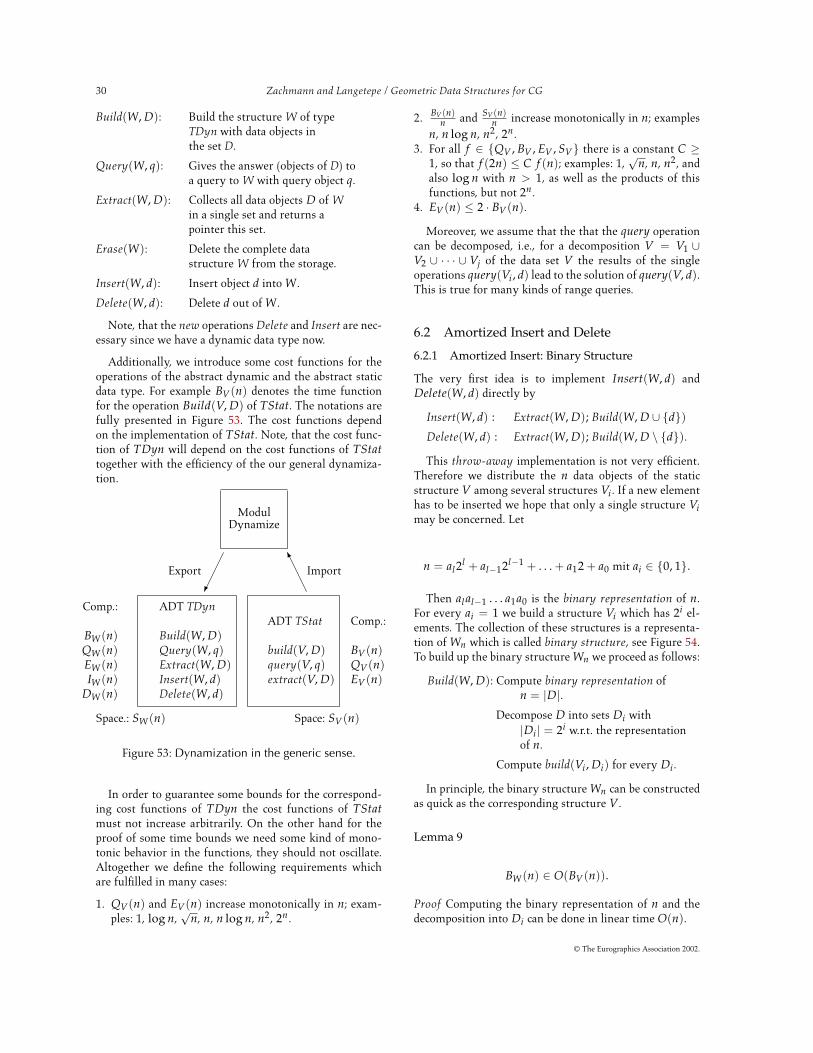
30 Zachmann and Langetepe / Geometric Data Structures for CG
Build(W, D): Build the structure W of typeTDyn with data objects inthe set D.
Query(W, q): Gives the answer (objects of D) toa query to W with query object q.
Extract(W, D): Collects all data objects D of Win a single set and returns apointer this set.
Erase(W): Delete the complete datastructure W from the storage.
Insert(W, d): Insert object d into W.
Delete(W, d): Delete d out of W.
Note, that the new operations Delete and Insert are nec-essary since we have a dynamic data type now.
Additionally, we introduce some cost functions for theoperations of the abstract dynamic and the abstract staticdata type. For example BV(n) denotes the time functionfor the operation Build(V, D) of TStat. The notations arefully presented in Figure 53. The cost functions dependon the implementation of TStat. Note, that the cost func-tion of TDyn will depend on the cost functions of TStattogether with the efficiency of the our general dynamiza-tion.
ModulDynamize
Comp.:
BW(n)QW(n)EW(n)IW(n)
DW(n)
ADT TDyn
Build(W, D)Query(W, q)Extract(W, D)Insert(W, d)Delete(W, d)
ADT TStat
build(V, D)query(V, q)extract(V, D)
Comp.:
BV(n)QV(n)EV(n)
Space.: SW(n) Space: SV(n)
KImport
®Export
Figure 53: Dynamization in the generic sense.
In order to guarantee some bounds for the correspond-ing cost functions of TDyn the cost functions of TStatmust not increase arbitrarily. On the other hand for theproof of some time bounds we need some kind of mono-tonic behavior in the functions, they should not oscillate.Altogether we define the following requirements whichare fulfilled in many cases:
1. QV(n) and EV(n) increase monotonically in n; exam-ples: 1, log n,
√n, n, n log n, n2, 2n.
2. BV (n)n and SV (n)
n increase monotonically in n; examplesn, n log n, n2, 2n.
3. For all f ∈ QV , BV , EV , SV there is a constant C ≥1, so that f (2n) ≤ C f (n); examples: 1,
√n, n, n2, and
also log n with n > 1, as well as the products of thisfunctions, but not 2n.
4. EV(n) ≤ 2 · BV(n).
Moreover, we assume that the that the query operationcan be decomposed, i.e., for a decomposition V = V1 ∪V2 ∪ · · · ∪ Vj of the data set V the results of the singleoperations query(Vi , d) lead to the solution of query(V, d).This is true for many kinds of range queries.
6.2 Amortized Insert and Delete
6.2.1 Amortized Insert: Binary Structure
The very first idea is to implement Insert(W, d) andDelete(W, d) directly by
Insert(W, d) : Extract(W, D); Build(W, D ∪ d)Delete(W, d) : Extract(W, D); Build(W, D \ d).
This throw-away implementation is not very efficient.Therefore we distribute the n data objects of the staticstructure V among several structures Vi. If a new elementhas to be inserted we hope that only a single structure Vimay be concerned. Let
n = al2l + al−12l−1 + . . . + a12 + a0 mit ai ∈ 0, 1.
Then al al−1 . . . a1a0 is the binary representation of n.For every ai = 1 we build a structure Vi which has 2i el-ements. The collection of these structures is a representa-tion of Wn which is called binary structure, see Figure 54.To build up the binary structure Wn we proceed as follows:
Build(W, D): Compute binary representation ofn = |D|.
Decompose D into sets Di with|Di | = 2i w.r.t. the representationof n.
Compute build(Vi , Di) for every Di.
In principle, the binary structure Wn can be constructedas quick as the corresponding structure V.
Lemma 9
BW(n) ∈ O(BV(n)).
Proof Computing the binary representation of n and thedecomposition into Di can be done in linear time O(n).
© The Eurographics Association 2002.

Zachmann and Langetepe / Geometric Data Structures for CG 31
24
23
22
21
20W23 W24
V0
V1
V2
V4 V4
V3
Figure 54: The binary structure Wn contains the structure Vi if ai = 1 holds for the binaryrepresentation of n. For examples see n = 23 (left) and n = 24 (right).
The operation build(Vi , Di) needs BV(2i) time. We havei ≤ l = blog nc and therefore we conclude:
blog nc∑i=0
BV(2i) =blog nc∑i=0
2i BV(2i)2i
≤blog nc∑i=0
2i BV(n)n
≤ 2log n BV(n)n
∈ O(BV(n)).
We used the fact that BV (n)n increases monotonically.
Altogether we have
BW(n) ∈ O(n + BV(n)) = O(BV(n))
since BV(n) is at least linear.
Similar results hold for some other operations. We canprove
EW(n) ≤ log n EV(n)
since we have to collect the results of extraxt(Vi) for atmost log n structures Vi.
Additionally,
QW(n) ≤ log n Qv(n)
holds if we assume that the query can be decompose aswell, see the requirements.
It is also easy to see that
SW(n) ≤blog nc∑i=0
SV(2i) ∈ O(SV(n)).
Therefore it remains to analyse IW(n).
As we have seen from Figure 54 sometimes the wholestructure of Wn is destroyed when Wn+1 was build up. Inthis example we had to perform the following tasks:
extract(V0 , D0); extract(V1 , D1); extract(V2 , D2);D := D0 ∪ D1 ∪ D2 ∪ d;build(V3 , D);
In general we have to build up Vj and extract and eraseVj−1, Vj−2, . . ., V0 only if ai = 1 holds for i = 0, 1 . . . , j−1 and aj = 0 holds (in the binary representation of thecurrent n).
In this special case we have
IW(n) ≤(
j−1
∑i=0
EV(2i)
)+ Cj + BV(2j)
≤ EV(2j) + Cj + BV(2j)
∈ O(
BV(2j))
.
For a long sequence of insertions many of them are per-formed without extreme reconstructions. Thus the effortfor all Insert(W, d) is amortized over time.
Generally, let Work be an arbitrary operation with costfunction W. For a sequence of s different operations letWork be applied k times. If
total cost of k Work operationenk
≤ W(s)
holds for a monotonically increasing cost function W, wesay that the operation Work is performed in amortizedtime W(s).
Note, that this is not an expected value and that W isa function of s, i.e., the length of the operation sequence.The current data set may have a number of elements n ≤s.
© The Eurographics Association 2002.

32 Zachmann and Langetepe / Geometric Data Structures for CG
For the Insert(W, d) operation one can prove
IW(s) ∈ O(
log ss
BV(s))
.
Note, that except insertions there are only queries in s.Queries do not change the size of the data set and so wecan also replace s by the number of insertions here.
Altogether, the results are presented in the followingtheorem.
Theorem 10A static abstract data type as presented in Figure 53 can bedynamized by means of the binary structure in a dynamicabstract data type TDyn so that the operation Insert(W, d)is performed in amortized time
IW(s) ∈ O(
log ss
BV(s))
.
Let n be the size of the current data set. We have
SW(n) ∈ log n Sv(n)
BW(n) ∈ BV(n))
QW(n) ∈ log n Qv(n).
6.2.2 Amortized Delete: Occasional Reconstruction
Assume that we did not have implemented the Insert op-eration, yet.
If we have to delete an object we can not choose itslocation beforehand. Therefore the deletion of an objectsis much more difficult than the insertion. Deletion maycause fundamental reconstruction.
For many data structures it is easier to simply markan object as deleted. Physically the object remains in thestructure but does no longer belong to the data set D.These objects have bad influence on the running time of alloperations although they are no longer necessary. There-fore from time to time we have to reconstruct the datastructure for the actual data set.
First of all for TStat we introduce an additional oper-ation weak.delete(V, d) with cost function WDV(n). Wesimply want to construct a strong delete function with anacceptable amortized time bound for TDyn.
Therefore we use weak.delete(V, d) until D has only thehalf size of V. Then we erase V and build a new struc-ture V out of D. The cost of the occasional reconstructionis amortized over the preceeding delete-operations. Thisgives the following result.
Theorem 11A static abstract data type as presented in Figure 53 with anadditional weak.delete(V, d) operation and with additional
cost function WDV(n) can be dynamized by means of oc-casional reconstruction in a dynamic abstract data typeTDyn so that
BW(r) = BV(r)EW(r) ∈ O (EV(r))QW(r) ∈ O (QV(r))SW(r) ∈ O (SV(r))
DW(s) ∈ O(
WDV(s) +BV(s)
s
),
holds. The size of the current actual data set is denotedwith r and s denotes the length of the operation sequence.
We omit the proof here.
6.2.3 Amortized Insert and Amortized Delete
In the preceeding sections we have discussed Insert andDelete separately. Now we want to show how to combinethe two approaches.
A static abstract data type with a weak delete imple-mentation is given. As in Section 6.2.1 we use the binarystructure for the insertion. The operation weak.delete isonly available for the structures Vi and we have to ex-tend it to W in order to apply the result of Section 6.2.2.If Weak.Delete(W, d) is applied, d should be marked asdeleted in W. But we do not know in which of the struc-tures Vi the element d lies. Therefore in addition to thebinary structure we construct a balanced searchtree T thatstores this information. For every d ∈ W there is a pointerto the structure Vi with d ∈ Vi, see Figure 55 for an exam-ple.
The additional cost of the search tree T is cov-ered as follows. Query operations are not involved. ForWeak.Delete(W, d) there is an additional O(log n) forsearching the corresponding Vi and for marking d asdeleted in Vi.
If an object d has to be inserted we have to update T.The object d gets an entry for its structure Vj in T, thisis done in time O(log n) and it will not affect the timebound for the insertion. But furthermore if V0 , . . . , Vj−1has to be erased the corresponding objects should point toVj afterwards. This can be efficiently realized by collectingthe pointers of T to Vi in a list for every Vi. We collectthe pointers and change them to "‘Vj"’. This operation is
already covered by time O(BV(2j)) for constructing Vj.
Altogether we conclude:
Theorem 12A static abstract data type as presented in Figure 53 with anadditional weak.delete(V, d) operation and with additionalcost function WDV(n) can be dynamized by means of bi-nary structure, searchtree T and occasional reconstruction
© The Eurographics Association 2002.

Zachmann and Langetepe / Geometric Data Structures for CG 33
15
13
9
1 2 3 4 5 6 7 8
14
10 11 12T
V3
V0
V1
V2
Figure 55: A structure W15 with a searchtree T storing pointers to Vi for every d ∈ Vi.
in a dynamic abstract data type TDyn so that the amor-tized time for insertion reads
IW(s) ∈ O(
log sBV(s)
s
),
and the amortized time for deletion reads
DW(s) ∈ O(
log s + WDV(s) +BV(s)
s
).
For the rest of the operations we have
BW(r) = BV(r)EW(r) ∈ O (log r EV(r))QW(r) ∈ O (log r QV(r))SW(r) ∈ O (SV(r)) .
The size of the current actual data set is denoted with r ands denotes the length of the operation sequence.
6.3 Worst-Case sensitive Insert and Delete
In the last section we have seen that it is easy to amor-tize the cost of Insert and Delete analytically over time.The main idea for the construction of the dynamic datastructure was given by the binary structure of Wn whichhas fundamental changes from time to time but the corre-sponding costs were amortized. Now we are looking forthe worst-case cost of Insert and Delete. The idea is todistribute the construction of Vj itself over time, i.e., thestructure Vj should be finished if Vj−1, Vj−2, . . . V0 has tobe erased.
We only refer to the result of this approach. The ideasare very similar to the ideas of the preceeding sections.Technically, a modified binary representation is used inorder to distribute the effort of the reconstruction overtime. For the interested reader we refer to Klein38 orvan Kreveld61 and Overmars51.
Theorem 13A static abstract data type as presented in Figure 53 with anadditional weak.delete(V, d) operation and with additional
cost function WDV(n) can be dynamized in a dynamic ab-stract data type TDyn so that
Build(W, D) ∈ O(BV(n))Query(W, q) ∈ O(log n ·QV(n))Insert(W, d) ∈ O
(log n
n BV(n))
Delete(W, d) ∈ O(
log n + WDV(n) + BV (n)n
)
Space O(SV(n)).
Here n denotes the number of relevant, stored data ob-jects.
6.4 A Simple Example
For convenience, we take a simple example from Section 2and apply Theorem 13, thus implementing worst-case sen-sitive insertion and deletion.
In Section 2.2 an easy implementation of the static k-d-tree was presented with Sk-d(n) = O(n) and query timeQk-d(n) = O(
√n + a), where a represents the size of
the answer, see Theorem 4. Obviously, weak.delete(k-d, x)can be implemented in O(log n) time, thus WDk-d(n) =O(log n). Additionally we have Bk-d(n) = O(n log n).
Let Dyn(k-d) denote the dynamic variant based uponthe statically implemented k-d-tree.
Application of Theorem 13 results in:
Build(Dyn(k-d), D) ∈ O(n log n)Query(Dyn(k-d), q) ∈ O(
√n log n + a)
Insert(Dyn(k-d), d) ∈ O(
log2 n)
Delete(Dyn(k-d), d) ∈ O (log n)Space O(n).
References
1. J. Arvo and D. B. Kirk, Fast Ray Tracingby Ray Classification, in Computer Graphics (SIG-GRAPH ’87 Proceedings), M. C. Stone, ed., vol. 21,July 1987, pp. 55–64. 11
2. F. Aurenhammer, Voronoi diagrams: A surveyof a fundamental geometric data structure, ACMComput. Surv., 23 (1991), pp. 345–405. 21
© The Eurographics Association 2002.

34 Zachmann and Langetepe / Geometric Data Structures for CG
3. F. Aurenhammer and R. Klein, Voronoi Di-agrams, in Handbook of Computational Geometry, J.-R. Sack and J. Urrutia, eds., Elsevier Science Publish-ers B.V. North-Holland, Amsterdam, 2000, pp. 201–290. URL http://wwwpi6.fernuni-hagen.de/
Publikationen/tr198.pdf. 21, 22, 23, 24
4. J. Avro and D. Kirk, A survey of ray tracingacceleration techniques, in An Introduction to RayTracing, A. Glassner, ed., Academic Press, San Diego,CA, 1989, pp. 201–262. ISBN 0-12-286160-4. 11, 17
5. L. Balmelli, J. Kovacevic, and M. Vet-terli, Quadtrees for Embedded Surface Visualiza-tion: Constraints and Efficient Data Structures, inProc. of IEEE International Conference on Image Pro-cessing (ICIP), vol. 2, Oct. 1999, pp. 487–491. 8
6. L. Balmelli, T. Liebling, and M. Vet-terli, Computational Analysis of 4-8 Meshes withApplication to Surface Simplification using global Er-ror, in Proc. of the 13th Canadian Conference onComputational Geometry (CCCG), Aug. 2001. 8
7. G. Barequet, B. Chazelle, L. J. Guibas,J. S. B. Mitchell, and A. Tal, BOX-TREE: A Hierarchical Representation for Surfaces in3D, Computer Graphics Forum, 15 (1996), pp. C387–C396, C484. ISSN 0167-7055. 17
8. N. Beckmann, H.-P. Kriegel, R. Schnei-der, and B. Seeger, The R∗-tree: An efficientand robust access method for points and rectangles,in Proc. ACM SIGMOD Conf. on Management ofData, 1990, pp. 322–331. 20
9. J. Bernal, Bibliographic notes on Voronoi dia-grams, tech. rep., National Institute of Standards andTechnology, Gaithersburg, MD 20899, 1992. 21
10. J.-D. Boissonnat and M. Teillaud,On the randomized construction of the Delaunaytree, Theoret. Comput. Sci., 112 (1993), pp. 339–354. URL http://www.inria.fr/cgi-bin/wais_
ra_sophia?question=1140. 24
11. P. J. C. Brown, Selective Mesh Refinementfor Rendering, PhD dissertation, Emmanuel Col-lege, University of Cambridge, Feb. 1998. URLhttp://www.cl.cam.ac.uk/Research/Rainbow/
publications/pjcb/thesis/. 6
12. N. Chin, Partitioning a 3D Convex Polygon withan Arbitrary Plane, in Graphics Gems III, D. Kirk,ed., Academic Press, 1992, chapter V.2, pp. 219–222.16
13. M. de Berg, M. van Kreveld, M. Over-mars, and O. Schwarzkopf, ComputationalGeometry: Algorithms and Applications, Springer-Verlag, Berlin, Germany, 2nd ed., 2000. 3, 5, 13, 23
14. F. Dehne and H. Noltemeier, A compu-tational geometry approach to clustering problems,in Proc. 1st Annu. ACM Sympos. Comput. Geom.,1985, pp. 245–250. 27
15. A. K. Dewdney and J. K. Vranch, A con-vex partition of R3 with applications to Crum’s prob-lem and Knuth’s post-office problem, Utilitas Math.,12 (1977), pp. 193–199. 24
16. H. Djidjev and A. Lingas, On computing theVoronoi diagram for restricted planar figures, in Proc.2nd Workshop Algorithms Data Struct., vol. 519 ofLecture Notes Comput. Sci., Springer-Verlag, 1991,pp. 54–64. 23
17. D. P. Dobkin and M. J. Laszlo, Primitivesfor the manipulation of three-dimensional subdivi-sions, Algorithmica, 4 (1989), pp. 3–32. 24
18. R. A. Dwyer, Higher-dimensional Voronoi di-agrams in linear expected time, Discrete Comput.Geom., 6 (1991), pp. 343–367. 24
19. H. Edelsbrunner, Algorithms in CombinatorialGeometry, vol. 10 of EATCS Monographs on The-oretical Computer Science, Springer-Verlag, Heidel-berg, West Germany, 1987. 21, 26
20. H. Edelsbrunner and N. R. Shah, Incre-mental topological flipping works for regular trian-gulations, Algorithmica, 15 (1996), pp. 223–241. 25
21. S. A. Ehmann and M. C. Lin, Accurate andFast Proximity Queries Between Polyhedra UsingConvex Surface Decomposition, in Computer Graph-ics Forum, vol. 20, 2001, pp. 500–510. ISSN 1067-7055. 21
22. A. A. Elassal and V. M. Caruso, USGSdigital cartographic data standards - Digital Eleva-tion Models, Technical Report Geological Survey Cir-cular 895-B, US Geological Survey, 1984. 5
23. D. A. Field, Implementing Watson’s algorithm inthree dimensions, in Proc. 2nd Annu. ACM Sympos.Comput. Geom., 1986, pp. 246–259. 25
24. S. Fortune, Voronoi diagrams and Delaunay tri-angulations, in Computing in Euclidean Geometry,D.-Z. Du and F. K. Hwang, eds., vol. 1 of LectureNotes Series on Computing, World Scientific, Singa-pore, 1st ed., 1992, pp. 193–233. 21
25. H. Fuchs, Z. M. Kedem, and B. F. Nay-lor, On Visible Surface Generation by a Priori TreeStructures, in Computer Graphics (SIGGRAPH ’80Proceedings), vol. 14, July 1980, pp. 124–133. 14
26. D. Fussell and K. R. Subramanian, FastRay Tracing Using K-D Trees, Technical Report TR-88-07, U. of Texas, Austin, Dept. Of Computer Sci-ence, Mar. 1988. 20
© The Eurographics Association 2002.

Zachmann and Langetepe / Geometric Data Structures for CG 35
27. A. S. Glassner, ed., An Introduction to RayTracing, Academic Press, 1989. 9
28. J. Goldsmith and J. Salmon, AutomaticCreation of Object Hierarchies for Ray Tracing,IEEE Computer Graphics and Applications, 7 (1987),pp. 14–20. 20
29. S. Gottschalk, M. Lin, andD. Manocha, OBB-Tree: A Hierarchical Struc-ture for Rapid Interference Detection, in SIGGRAPH96 Conference Proceedings, H. Rushmeier, ed., An-nual Conference Series, ACM SIGGRAPH, AddisonWesley, Aug. 1996, pp. 171–180. held in NewOrleans, Louisiana, 04-09 August 1996. 17, 18, 20,21
30. L. J. Guibas and J. Stolfi, Primitives for themanipulation of general subdivisions and the com-putation of Voronoi diagrams, ACM Trans. Graph., 4(1985), pp. 74–123. 23
31. H. W. Hamacher, Mathematische Lösungsver-fahren für planare Standortprobleme, VerlagVieweg, Wiesbaden, 1995. 27
32. P. M. Hubbard, Real-Time Collision Detectionand Time-Critical Computing, in SIVE 95, The FirstWorjshop on Simulation and Interaction in VirtualEnvironments, no. 1, Iowa City, Iowa, July 1995, Uni-versity of Iowa, informal proceedings, pp. 92–96. 21
33. H. Inagaki, K. Sugihara, and N. Sugie,Numerically robust incremental algorithm for con-structing three-dimensional Voronoi diagrams, inProc. 4th Canad. Conf. Comput. Geom., 1992,pp. 334–339. 25
34. B. Joe, 3-Dimensional Triangulations from LocalTransformations, SIAM J. Sci. Statist. Comput., 10(1989), pp. 718–741. 25
35. , Construction of Three-Dimensional Delau-nay Triangulations Using Local Transformations,Comput. Aided Geom. Design, 8 (1991), pp. 123–142.25
36. N. Katayama and S. Satoh, The SR-tree:An Index Structure for High-Dimensional NearestNeighbor Queries, in Proc. ACM SIGMOD Conf. onManagement of Data, 1997, pp. 369–380. 17
37. T. L. Kay and J. T. Kajiya, Ray TracingComplex Scenes, in Computer Graphics (SIGGRAPH’86 Proceedings), D. C. Evans and R. J. Athay, eds.,vol. 20, Aug. 1986, pp. 269–278. 17
38. R. Klein, Algorithmische Geometrie, Addison-Wesley, Bonn, 1997. URL http://www.
oldenbourg.de/cgi-bin/rotitel?T=24382.3, 29, 33
39. J. T. Klosowski, M. Held, J. S.Mitchell, H. Sowrizal, and K. Zikan,Efficient Collision Detection Using Bounding VolumeHierarchies of k-DOPs, IEEE Transactions on Visual-ization and Computer Graphics, 4 (1998), pp. 21–36.17, 21
40. T. Larsson and T. Akenine-Mller, Col-lision Detection for Continuously Deforming Bodies,in Eurographics, 2001, pp. 325–333. short presenta-tion. 21
41. C. L. Lawson, Software for C1 surface interpola-tion, in Math. Software III, J. R. Rice, ed., AcademicPress, New York, NY, 1977, pp. 161–194. 23
42. S. Leutenegger, J. Edgington, andM. Lopez, STR : A Simple and Efficient Algorithmfor R-Tree Packing, in Proceedings of the 13th Inter-national Conference on Data Engineering (ICDE’97),Washington - Brussels - Tokyo, Apr. 1997, IEEE,pp. 497–507. ISBN 0-8186-7807-0. 19
43. T.-Y. Li and J.-S. Chen, Incremental 3D Col-lision Detection with Hierarchical Data Structures,in Proc. VRST ’98, Taipei, Taiwan, Nov. 1998, ACM,pp. 139–144. 21
44. P. Lindstrom, D. Koller, W. Ribarsky,L. F. Hughes, N. Faust, and G. Turner,Real-Time, Continuous Level of Detail Rendering ofHeight Fields, in SIGGRAPH 96 Conference Pro-ceedings, H. Rushmeier, ed., Annual Conference Se-ries, ACM SIGGRAPH, Addison Wesley, Aug. 1996,pp. 109–118. held in New Orleans, Louisiana, 04-09August 1996. 5, 8
45. P. Lindstrom and V. Pascucci, Visualiza-tion of Large Terrains Made Easy, in Proc. IEEE Vi-sualization, San Diego, 2001. 6, 7, 8
46. W. E. Lorensen and H. E. Cline, March-ing Cubes: A High Resolution 3D Surface Construc-tion Algorithm, in Computer Graphics (SIGGRAPH’87 Proceedings), M. C. Stone, ed., vol. 21, July 1987,pp. 163–169. 8
47. G. Mller, S. Schfer, and W. D. Fell-ner, Automatic Creation of Object Hierarchies forRadiosity Clustering, Computer Graphics Forum, 19(2000). ISSN 0167-7055. 20
48. B. Naylor, J. Amanatides, andW. Thibault, Merging BSP Trees YieldsPolyhedral Set Operations, in Computer Graphics(SIGGRAPH ’90 Proceedings), F. Baskett, ed., vol. 24,Aug. 1990, pp. 115–124. 15
49. B. F. Naylor, A Tutorial on Binary Space Par-titioning Trees, ACM SIGGRAPH ’96 Course Notes29, (1996). 14, 15
© The Eurographics Association 2002.

36 Zachmann and Langetepe / Geometric Data Structures for CG
50. R. Osada, T. Funkhouser, B. Chazelle,and D. Dobkin, Matching 3D models withshape distributions, in Proceedings of the Interna-tional Conference on Shape Modeling and Applica-tions (SMI-01), B. Werner, ed., Los Alamitos, CA,May 7–11 2001, IEEE Computer Society, pp. 154–166.29
51. M. H. Overmars, The Design of Dynamic DataStructures, vol. 156 of Lecture Notes Comput. Sci.,Springer-Verlag, Heidelberg, West Germany, 1983.29, 33
52. I. J. Palmer and R. L. Grimsdale, Col-lision Detection for Animation using Sphere-Trees,Computer Graphics Forum, 14 (1995), pp. 105–116.ISSN 0167-7055. 21
53. M. S. Paterson and F. F. Yao, Efficient bi-nary space partitions for hidden-surface removal andsolid modeling, Discrete Comput. Geom., 5 (1990),pp. 485–503. 13
54. F. P. Preparata and M. I. Shamos, Com-putational Geometry: An Introduction, Springer-Verlag, New York, NY, 1985. 21
55. V. T. Rajan, Optimality of the Delaunay trian-gulation in Rd, in Proc. 7th Annu. ACM Sympos.Comput. Geom., 1991, pp. 357–363. 25
56. J. Revelles, C. Urena, and M. Las-tra, An Efficient Parametric Algorithm for OctreeTraversal, in WSCG 2000 Conference Proceedings,2000. URL http://visinfo.zib.de/EVlib/Show?
EVL-2000-307. 10
57. N. Roussopoulos and D. Leifker, Directspatial search on pictorial databases using packedR-trees, in Proceedings of ACM-SIGMOD 1985International Conference on Management of Data,May 28–31, 1985, LaMansion Hotel, Austin, Texas,S. Navathe, ed., New York, NY 10036, USA, 1985,ACM Press, pp. 17–31. ISBN 0-89791-160-1. LCCNQA 76.9 D3 I59 1985; QA1 .A87. URL http://www.
acm.org/pubs/articles/proceedings/mod/
318898/p17-roussopoulos/p17-roussopoulos.
pdf;http://www.acm.org/pubs/citations/
proceedings/mod/318898/p17-roussopoulos/.19
58. M. I. Shamos, Computational Geometry, ph.D.thesis, Dept. Comput. Sci., Yale Univ., New Haven,CT, 1978. 23
59. M. Tanemura, T. Ogawa, and W. Ogita,A New Algorithm for Three-Dimensional VoronoiTesselation, J. Comput. Phys., 51 (1983), pp. 191–207.25
60. G. van den Bergen, Efficient Collision Detec-
tion of Complex Deformable Models using AABBTrees, Journal of Graphics Tools, 2 (1997), pp. 1–14.21
61. M. J. van Kreveld, New Results on DataStructures in Computational Geometry, ph.D. dis-sertation, Dept. Comput. Sci., Utrecht Univ., Utrecht,Netherlands, 1992. 29, 33
62. D. F. Watson, Computing the n-DimensionalDelaunay Tesselation with Applications to VoronoiPolytopes, Comput. J., 24 (1981), pp. 167–172. 25
63. H. Weghorst, G. Hooper, and D. P.Greenberg, Improved Computational Methodsfor Ray Tracing, ACM Transactions on Graphics, 3(1984), pp. 52–69. 17
64. L.-Y. Wei and M. Levoy, Fast Texture Syn-thesis Using Tree-Structured Vector Quantization,in Siggraph 2000, Computer Graphics Proceedings,K. Akeley, ed., Annual Conference Series, ACM Press/ ACM SIGGRAPH / Addison Wesley Longman,2000, pp. 479–488. URL http://visinfo.zib.de/
EVlib/Show?EVL-2000-87. 27, 28
65. J. Wilhelms and A. V. Gelder, Octreesfor Faster Isosurface Generation Extended Abstract,in Computer Graphics (San Diego Workshop on Vol-ume Visualization), vol. 24, Nov. 1990, pp. 57–62. 9
66. G. Zachmann, Real-time and Exact Collision De-tection for Interactive Virtual Prototyping, in Proc. ofthe 1997 ASME Design Engineering Technical Con-ferences, Sacramento, California, Sept. 1997. Paperno. CIE-4306. 21
67. , Rapid Collision Detection by DynamicallyAligned DOP-Trees, in Proc. of IEEE Virtual RealityAnnual International Symposium; VRAIS ’98, At-lanta, Georgia, Mar. 1998, pp. 90–97. 17, 21
68. B. Zhu and A. Mirzaian, Sorting does not al-ways help in computational geometry, in Proc. 3rdCanad. Conf. Comput. Geom., Aug. 1991, pp. 239–242. 23
© The Eurographics Association 2002.