geometric (classical) multigrid. hierarchy of graphs apply grids in all scales: 2x2, 4x4, …, n 1/2...
TRANSCRIPT

Geometric (Classical) MultiGrid

Hierarchy of
graphs
Apply grids in all scales: 2x2, 4x4, … , n1/2xn1/2
Coarsening Interpolate and relax
Solve the large systems of equations by multigrid!
G1
G2
G3
Gl
G1
G2
G3
Gl

Linear (2nd order) interpolation in 1D
x1 x2x
F(x)
)()()( 212
11
12
2 xFxx
xxxF
xx
xxxF

i
S(i)
(Ulb,Vlb)
(Urt,Vrt)(Ult,Vlt)
(Urb,Vrb)
(x2,y2)(x1,y2)
(x2,y1)(x1,y1)
(x0,y0)
Bilinear interpolation
C(S(i))={rb,rt,lb,lt}

i
S(i)
(Ulb,Vlb)
(Urt,Vrt)(Ult,Vlt)
(Urb,Vrb)
(x2,y2)(x1,y2)
(x2,y1)(x1,y1)
(x0,y0)
lbltlrbrtr UUUUyy
yyU
yy
yyU ......;
12
02
12
10
(Ul,Vl) (Ur,Vr)
lr Uxx
xxU
xx
xxyxU
12
02
12
1000 ),(

From (x,y) to (U,V) by bilinear intepolation
])~~(
)~~[(),(
])()[(),(
))((
2
))((
2
))(())((,
22
,
jscpjpjpj
iscpipipi
jscpjpjpj
iscpipipi
jiij
jijiji
ij
VyVy
UxUxaVUE
yyxxayxE

Linear scalar elliptic PDE (Brandt ~1971)
1 dimension Poisson equation
Discretize the continuum
LU )(xx F)(U 10 x
0)U()U( 10
x0 x1 x2 xi xN-1 xN
x=0 x=1h
Grid: ihxN
h i ,1
Ni 0
h
Let ihi FF local
averaging),( ixU )( ixFi
hi UU

Linear scalar elliptic PDE 1 dimension Laplace equation
Second order finite difference approximation
=> Solve a linear system of equationsNot directly, but iteratively=> Use Gauss Seidel pointwise relaxation
LU 0 )(U x 10 x
0)U()U( 10
hihUL 0
UUU
2
11 2
hiii 11 Ni
00 NUU

fine grid
h
u = average of u's
approximating Laplace eq.2 2
2 20
u u
x y
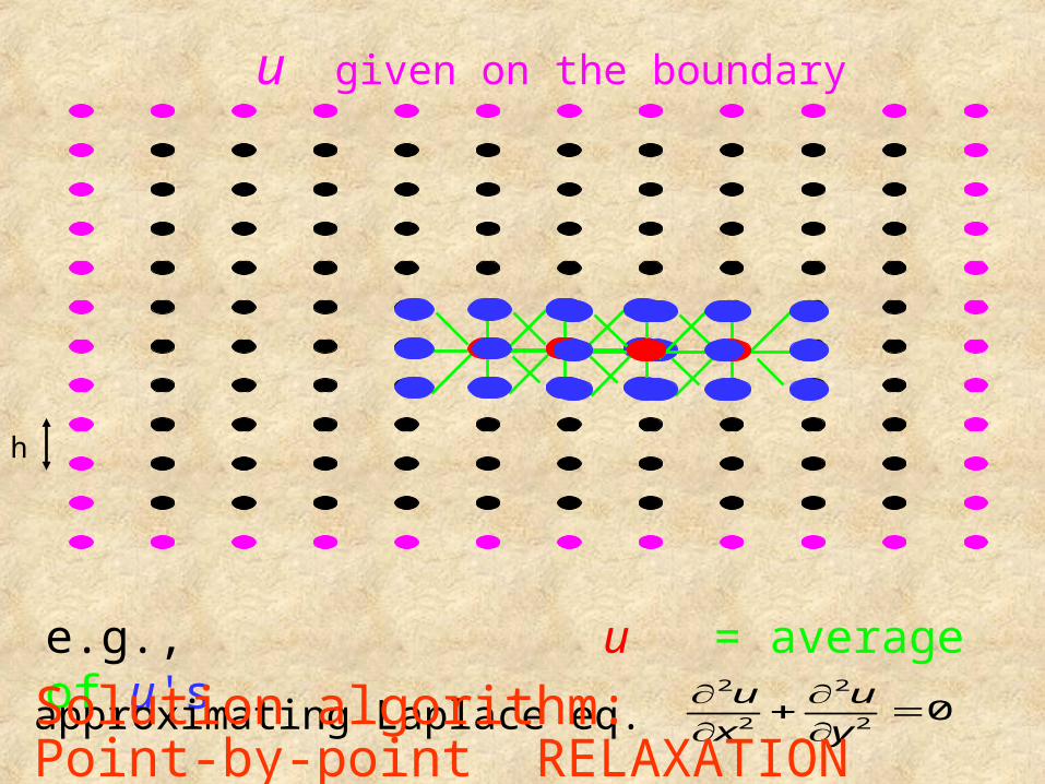
u given on the boundary
h
e.g., u = average of u's
approximating Laplace eq.2 2
2 20
u u
x y
Point-by-point RELAXATIONSolution algorithm:

Exc#9: Error calculations
1. Use Taylor expansion to calculate the error when U’’(x) is approximated by
2. Find a,b,c,d and e such that
This is a higher order approximation for U’’(x) than the one in exercise 1.
2
)()(2)(
h
hxUxUhxU
)()()2()()()()2( 4hOxUhxeUhxdUxcUhxbUhxaU
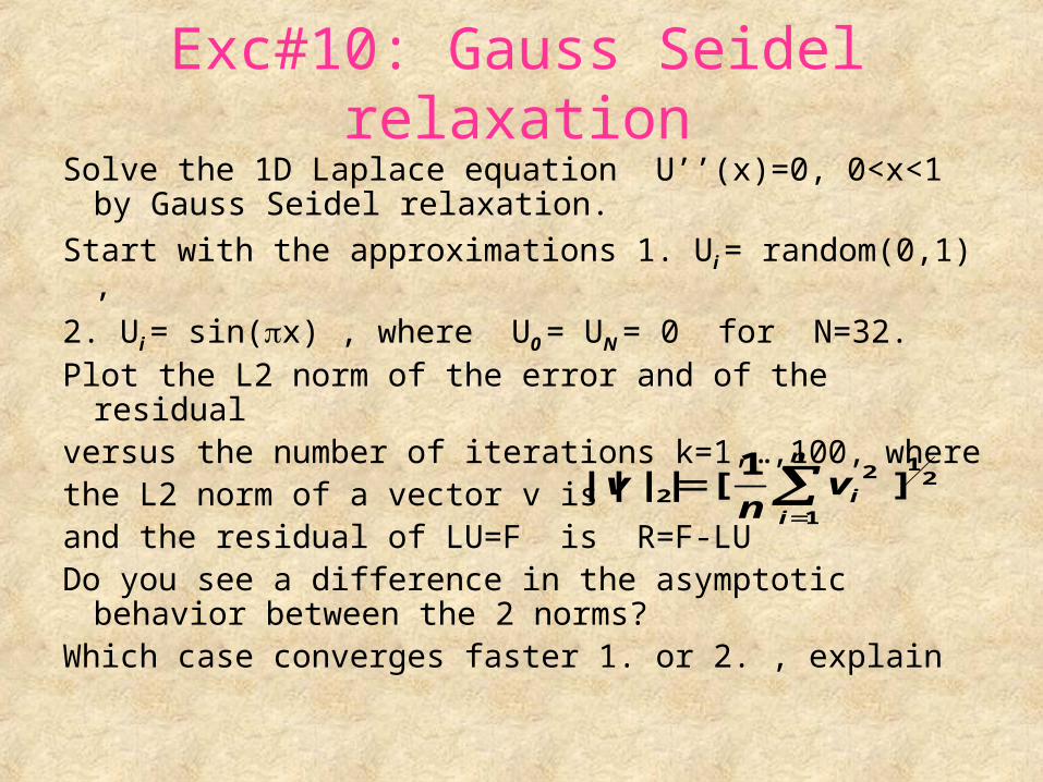
Exc#10: Gauss Seidel relaxation
Solve the 1D Laplace equation U’’(x)=0, 0<x<1 by Gauss Seidel relaxation.
Start with the approximations 1. Ui = random(0,1) ,
2. Ui = sin(x) , where U0 = UN = 0 for N=32.Plot the L2 norm of the error and of the residualversus the number of iterations k=1,…,100, wherethe L2 norm of a vector v isand the residual of LU=F is R=F-LUDo you see a difference in the asymptotic behavior
between the 2 norms?Which case converges faster 1. or 2. , explain
21
1
22 ]
1[||||
n
iivn
v

Influence of (pointwise) Gauss-Seidelrelaxation on the error
Poisson equation, uniform grid
Error of initial guess Error after 5 relaxation
Error after 10 relaxations Error after 15 relaxations

The basic observations of ML Just a few relaxation sweeps are needed to
converge the highly oscillatory components of the error
=> the error is smooth Can be well expressed by less variables Use a coarser level (by choosing every other
line) for the residual equation Smooth component on a finer level becomes
more oscillatory on a coarser level=> solve recursively The solution is interpolated and added
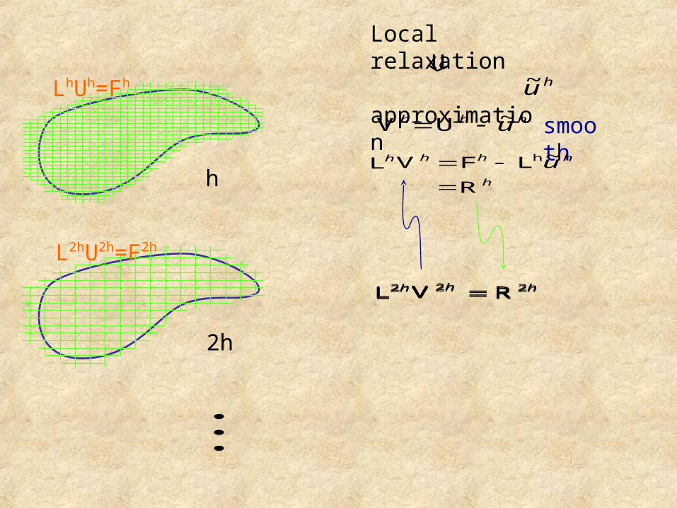
h
2h
Local relaxation
approximation
hu~
hV hh u~U smoothhh u~LF hhVhL
hR
h2Vh2L h2R
LhUh=Fh
L2hU2h=F2h
h2Vh2L h2R
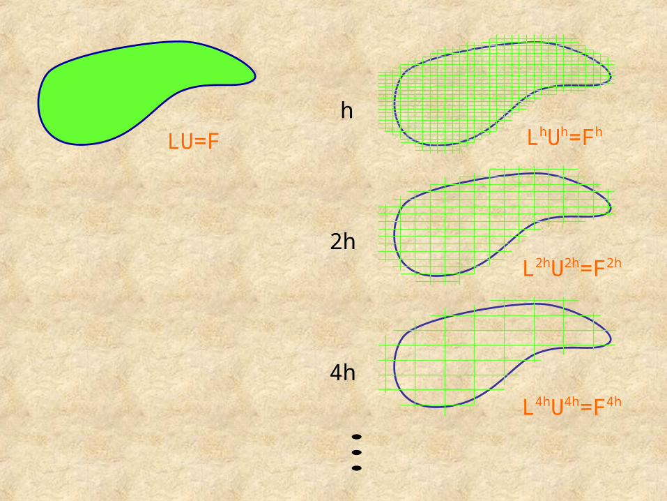
LU=Fh
2h
4h
LhUh=Fh
L2hU2h=F2h
L4hU4h=F4h

TWO GRID CYCLE
Approximate solution:hu~
hhh u~UV hhh RVL
hhhh u~LFR
Fine grid equation: hhh FUL
2. Coarse grid equation: hhh RVL 22
hh2
h2v~~~ hold
hnew uu h
h2
Residual equation:Smooth error:
1. Relaxation
residual:
h2v~Approximate solution:
3. Coarse grid correction:
4. Relaxation

Why additional relaxations are needed?

Why additional relaxations are needed?
A smooth approximation is obtained after relaxation on the finer level

Why additional relaxations are needed?
A smooth approximation is obtained after relaxation on the finer level
The coarse grid correction

Why additional relaxations are needed?
The coarse grid correction
Interpolate and add

Why additional relaxations are needed?
The coarse grid correction
Interpolate and add

Why additional relaxations are needed?
The coarse grid correction
Interpolate and add

Why additional relaxations are needed?
The coarse grid correction
Interpolate and add

Why additional relaxations are needed?
The coarse grid correction
Interpolate and add

Why additional relaxations are needed?
Interpolate and add => high oscillatory component emerges

TWO GRID CYCLE
Approximate solution:hu~
hhh u~UV hhh RVL
hhhh u~LFR
Fine grid equation: hhh FUL
2. Coarse grid equation: hhh RVL 22
hh2
hold
hnew uu h2v~~~ h
h2
Residual equation:Smooth error:
1. Relaxation
residual:
h2v~Approximate solution:
3. Coarse grid correction:
4. Relaxation
1
2
34
5
6
by recursion
MULTI-GRID CYCLE
Correction Scheme
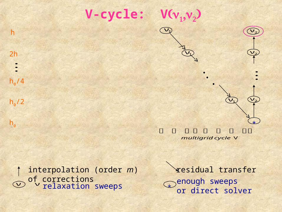
interpolation (order m)of corrections relaxation sweeps
residual transfer
ν ν enough sweepsor direct solver*
.. .
*
1ν
1ν
1ν
2ν
2ν
2ν
Vcyclemultigrid
h0
h0/2
h0/4
2h
h
V-cycle: V
Multigrid solversCost: 25-100 operations per unknown
• Linear scalar elliptic equation (Achi Brandt ~1971)

Multigrid solversCost: 25-100 operations per unknown
• Linear scalar elliptic equation (~1971)*• Nonlinear• Grid adaptation• General boundaries, BCs*• Discontinuous coefficients• Disordered: coefficients, grid (FE) AMG• Several coupled PDEs* (1980)
• Non-elliptic: high-Reynolds flow• Highly indefinite: waves• Many eigenfunctions (N)• Near zero modes• Gauge topology: Dirac eq.• Inverse problems• Optimal design• Integral equations Full matrix• Statistical mechanics
Massive parallel processing*Rigorous quantitative analysis (1986)
FAS (1975)
Within one solver
)log(
2
NNO
fuku
(1977,1982)