��������������� �������������

22

�����������������

The GeoMedia Fusion Validate Geometry command provides the GUI for detecting geometric anomalies on a single feature.

����������������������������������������

Below is a discussion of the Standard Advanced Validate Geometry types.

• Empty Geometry refers to features that have an empty geometry component. (e.g. A composite or collection without any components or a geometry that is returned as an empty variant).

• Unknown Geometry Type refers to those features whose geometry type does not correspond to a type recognized by GeoMedia. More specifically, when the top-level blob header does not conform to any of the geometry CLSID defined in GDO.

• Invalid Geometry refers to those features whose geometry type does not match the geometry’s delineation (e.g. an area whose subtype is not gdbAreal or gdbAnySpatial) or whose geometry specification is invalid for GeoMedia.

• Invalid Geometric Component refers to those features whose geometry is syntactically correct (i.e. passed the check as specified by the Invalid Geometry anomaly), but whose specification does not define a valid geometric component. Included in the definition of invalid geometries are the following:

Invalid Arc – the radius, start point, and end point are not valid.

Invalid Boundary - the boundaries exterior or interior components are not polygons.

Discontinuous Composite - the composite does not form a connected path.

• Uncontained Holes refers to area features with inner boundaries (holes) that are not contained (totally or partially) within the outer boundary.

• Unclosed Areas refers to area features whose boundary does not close. In other words, the first and last point of the boundary do not have the same coordinate values.

��������������� �������������

23

The process identifies the original feature geometry. Specifically, the first and last points of the boundary are identified. The anomaly geometry is a Geometry Collection containing two points corresponding to the first and last point of the area.

• Overlapping Holes refers to area features whose inner boundaries (holes) overlap one another.

• Zero-Length Lines refers to linear features whose coordinates all occupy the same xy location. The process identifies the original feature geometry. The anomaly geometry is a polyline containing the points in the original geometry.

• Zero-Coverage Areas refers to areas features that have no area (i.e. the vertices are all collinear). The process identifies the original feature geometry. The anomaly geometry is a polyline containing the points in the original geometry.

• Loop in Area refers to area features that contain a loop in either its outer or inner boundaries. No measurement is required as any loop is considered an anomaly.

• Kickback refers to linear or area features where the geometry doubles back on itself.

��������������� �������������

24

The line above is defined by a sequence of 10 vertices (A-B-C-D-C-D-E-F-G-H). The sequence D-C-D defines the kickback.

A kickback is corrected by removing the vertices that create the kickback. In the above example, the second set of vertices at C and D are removed. The line is defined by the sequence of 8 vertices (A-B-C-D-E-F-G-H). This is a simple case of a Kickback.

The process identifies the original feature geometry. Specifically, the vertex or set of two vertices that defined the kickback. The anomaly geometry is either a single point for a duplicate point (corresponds to the location of the duplicate point) or a Geometry Collection containing two vertices that represent the kickback.

������������������������������� ����������������

Below is a discussion of the Advanced Validate Geometry Specialized Anomaly types

• Kink (or Spike) refers to linear or area features where there is a sudden divergence of the vertices that define the geometry. A measurement is required to distinguish between kinks and what are considered normal characteristics of the feature.

In the above line, the vertex sequence A-B-C defines a sudden divergence of the line. This divergence can be a kink.

• Loop in Line refers to linear features whose geometry creates a loop whose area is greater than some specified tolerance.

��������������� �������������

25

Unlike Loop in Area, not all loops in line features are anomalies. Only those loops whose size is less than some specified parameter are considered anomalies.

In the above definition, small loops are considered anomalies, while larger ones are considered a normal characteristic. Since the loop is considered an abnormal characteristic, the vertices placed to create the loop can be considered as invalid. Removing these vertices and thus removing the loop can be considered the proper way to correct this anomaly.

• Short Vector refers to line or area features with two sequential vertices less than some user-specified tolerance from one another.

In the above example, the line has two sequential vertices (A and B) that are less than some specified tolerance from one another. This defines the Short Vector Anomaly.

Correcting the Short Vector anomaly requires removal of one of the vertices. Although subtle differences could result depending on which vertex is removed it appears that those differences can be ignored. In the above example, resolution is achieved by deleting point A.

• Fragmented Geometry refers to a feature whose geometry is a collection of distinct geometries. The collection could be any combination of area, lines and/or points. The geometries belonging to the collection do not need to be discontiguous for it to be considered a fragmented geometry anomaly. An automated resolution is available for those feature recordsets with an auto-number key field. If the recordset has a key field or fields other than auto-number, no automatic resolution is available. New records are created for each separate geometry in the collection. Optionally, the original record can be kept and used as one of the new features created. The attribute values for the new records are copied from the original record and a geometry is created that corresponds with one of the distinct elements in the collection. If the original record is kept, its geometry is modified to correspond to one of the geometry components.

• Duplicate Feature refers to two features whose attributes match and whose geometries are either identical or have similar size, shape, and location within some specified tolerance. The

��������������� �������������

26

example below illustrates two line and two area features whose geometries do not match, but which may still be considered duplicates.

Although the two line and area geometries above do not match exactly, they have similar size, shape, and location, and may be considered duplicates. Determination of whether two features are duplicates can be made by creating zones around the features and analyzing the spatial relationship of the two zones to one another. The picture below shows the lines above with buffer zones around each of them.

For points to be considered duplicates, one point only need be within the specified buffer distance of another for it to be considered a duplicate (i.e. no calculation of the overlap between the zones is required). The certainty value for a point being a duplicate of another is either 0 (not within buffer distance) or 100 (within buffer distance).

Due to the complexity of analyzing Geometry Collections, they will be considered for exact duplicates only at this time. Geometry Collections will not be processed for near duplicates.

The attribute check is performed optionally. Either all attributes must match for a feature to be considered a duplicate, or no attributes are checked, in which case the geometry only is processed. When attributes are checked, all fields with the exception of key fields and geometry fields must have the exact same values.

��������������� �������������

27

• Void Area refers to a bounded region that does not belong to any area feature. Void Area would be an anomaly for map data that is required to be continuous coverage.

In the example above, two area features are coincident in such a way as to create a bounded region that does not belong to either area feature. This bounded region is an example of a Void Area Anomaly. The unbounded regions of the data under consideration that do not belong to an area are not detected as a Void Area. The data would have to be modified so that these regions become bounded before they would be identified as a Void Area Anomaly.

The results are output as a query and can be displayed in a map window, data window, and/or queue. The command uses the AdvancedValidateGeometryPipe and the DuplicateFeaturePipe (through the AdvancedValidateGeometryProps Control) to determine the anomalies on the selected feature classes. Any changes to the geometries of the features for which anomalies are detected will automatically update in any open map or data windows and any dynamic queues.

• Superfluous Geometry refers to those instances where the geometry of a feature contains a component which is not needed to portray the feature. Included in Superfluous Geometry are zero-length arcs and composites or collections with only one component.

���������������������������������

1. Select Geomedia Professional and open the Geoworkspace of C:\Training/Buncombe/BuncombeCounty.gws.

2. Select Legend > Add Legend Entries and select the BuncombeCounty connection and the feature class of Road.

��������������� �������������

28

��������������� �������������

29

3. Select Toolbox > Geometric Validation > Validate Geometry.

4. Select the Input tab and select the BuncombeCounty connection feature class of Road.

��������������� �������������

30

5. Select the Anomalies tab and review the Standard and Specialized entries.

��������������� �������������

31

6. Check all of the Standard and Specialized entries.

7. Select the Output tab and keep the Output anomalies to queue checked to Queue of Anomalies and Output anomalies as query checked.

��������������� �������������

32

8. Select the OK button on the Advanced Validate Geometry dialog.

9. The Queued Edit Map Window, the Queued Edit Data Window, and the Queued Edit control will activate when the processing concludes.

10. Scroll through the Queued Edit list of Queue of Anomalies and review the detected Geometric anomalies.

��������������� �������������

33

11. Notice that Kinks, Duplicate Feature, Fragmented Geometry, and Null Geometry anomalies have been detected.

��������������� �������������

34

12. Select the Toolbox > Validate Geometry > Anomalies tab and check the Specialized Kink, Duplicate Feature, Fragmented Geometry, and Null Geometry options.

13. Select the Input tab and select the BuncombeCounty connection Road feature class.

��������������� �������������

35

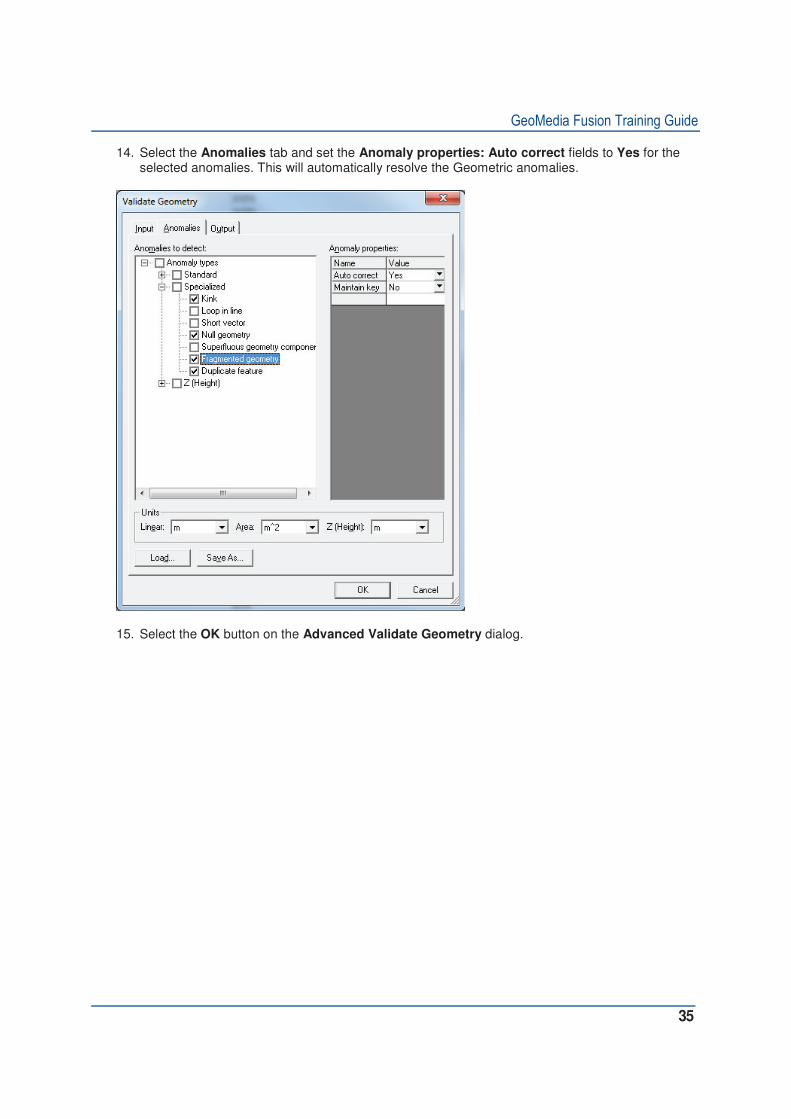
14. Select the Anomalies tab and set the Anomaly properties: Auto correct fields to Yes for the selected anomalies. This will automatically resolve the Geometric anomalies.

15. Select the OK button on the Advanced Validate Geometry dialog.

��������������� �������������

36

16. The Queued Edit Map Window, Queued Edit Data Window, and Queue of Anomalies are now redisplayed with 0 anomalies.

17. Close the Queued Edit Map Window and exit the Queued Edit command.

���������!���������������������������

�""��������#��$������������������%������������!���������

• GeoMedia Professional only allows for connectivity to be validated between two feature classes (a source and a target). Connectivity of the source feature is compared with the target feature. Fusion allows for connectivity between multiple feature classes to be checked. The connectivity of each feature in each class is checked between all other features in the specified classes.

• Fusion also provides an advanced feature selection mode where, depending on the anomaly type, connectivity is checked between two groups of feature classes.

• GeoMedia Pro checks for connectivity in a pair-wise fashion; one feature in the source feature class against one feature in the target feature class. This can result in over reporting due to the fact that other features in the target class are not checked simultaneously against the feature.

• More Fusion anomaly types are detected.

• An output to a queue option is available.

• GeoMedia Pro detects anomalies between features by a pair-wise analysis of the geometry. Only two geometries are compared at a time without regard to any other related geometries.

��������������� �������������

37

Undershoots

In the example below, feature A is connected to feature B, which then crosses feature C. A pair-wise analysis of the features as done in GM Professional leads to the conclusion that feature A undershoots feature C.

Fusion does not see this as an undershoot. It looks at the entire connected topological network and determines that no undershoot exists.

• Fusion looks at the geometry of all the features involved, not just a pair-wise analysis. This can cause the results returned by the products to vary.

• For those anomaly types that can be corrected, the user can specify to correct them as they are encountered, in which case they are not output to the queue.

Note that correction of the undershoot as done in GeoMedia Professional could lead to features A and B no longer remaining coincident at their endpoints. Since feature B is not considered, feature A is extended to feature C to correct the undershoot, causing the two features to no longer be connected at their endpoints.

Geomedia Pro looks for undershoots by taking an endpoint of a line and comparing with other features. If a line can be drawn normal to a segment on another feature and if the distance is less than the specified

��������������� �������������

38

tolerance, an undershoot is reported. Fusion measures the distance from the endpoint to the intersection of another segment along the original trend of the line. This difference can be outlined below.

Feature A is being compared against feature B for an undershoot. Geomedia Pro looks for the perpendicular distance between the endpoint of feature A and a segment on feature B. Because this perpendicular line does not intersect feature B, no undershoot is detected or reported. Fusion measures the distance along the original trend of the line (shown in green). If the distance from the endpoint to this intersection is less than the tolerance, an undershoot is reported.

In another example above, the endpoint of line A is within the specified distance (undershoot tolerance) of line C. Therefore, the relationship of line A to line C represents an undershoot. Line B is not within the specified tolerance of line C; therefore it is not an undershoot. The undershoot distance is calculated by projecting the line (Line A or Line B) along its original direction until it meets the undershot line (Line C). A perpendicular projection is not made.

Undershoots can be corrected by extending the line to meet the undershot line. (In this case, extending A to meet C). However not all situations are this straightforward, which could require the user to review and edit the features in order to resolve them.

The two features and the location are identified where the undershoot occurs. The endpoint of the undershooting feature along with location on the undershot feature where projection would occur.

Overshoots

Given the same example above, the effect of the pair-wise comparison can be seen for overshoots as well. A pair-wise analysis of the features as done in GM Pro leads to the conclusion that feature B overshoots feature C

��������������� �������������

39

Fusion does not see this as an overshoot. It looks at the entire connected network and makes the decision that no undershoot exists.

Correction of the overshoot of feature B to feature C would lead to a similar undesirable result where feature B is terminated at the intersection to feature C and becomes disconnected from feature A. Correcting undershoots and overshoots could lead to the following results for this case.

In another example (below), line A extends past line C a distance less than the specified distance (undershoot tolerance). Therefore, the relationship of line A to line C represents an overshoot. Line B extends past line C a distance greater than this tolerance, and therefore does not represent an overshoot.

Overshoots can be corrected by deleting the part of the line that extends past the overshot line. (In this case, deleting the part of line A that extends past C). However, not all situations are this straightforward, which could require the user to review and edit the features in order to resolve.

An overshoot could also be a case of Unbroken Intersecting Geometry. If this is the case, the overshoot should be corrected, which will in effect correct Unbroken Intersecting Geometry. An overshoot that is

Line A

Overshoot Tolerance

Line B

Line C

��������������� �������������

40

also an Unbroken Intersecting Geometry should be identified solely as an Overshoot and corrected as such.

An overshoot could and will in all likelihood be also Non-coincident. However correcting the overshoot will correct the Non-coincident Intersecting Geometry.

Node Mismatch

The effect of the pair-wise comparison for node mismatches does not cause Geomedia Professional to report anomalies that do not exist as for overshoots or undershoots. It does, however, cause anomalies to be over-reported.

In the above example, the endpoints of 2 lines are all within a specified node mismatch tolerance of one another. Because of the pair-wise comparison done in GeoMedia Professional, this one anomaly will be reported twice (AB, BA). Fusion would report this anomaly one time.

Only being able to select two feature classes and only comparing one feature class to another leads to different results for GeoMedia Professional than for Fusion.

In the above example, node B belongs to feature class 1, and is within the tolerance of both node A and node C of feature class 2. Node A and Node C are also within the node mismatch tolerance. GeoMedia Professional will report four node mismatches (AB, BA, BC, CB). It does not report AC as a mismatch, as they are from the same feature class.

Fusion processes the feature classes together, comparing FC1 to FC2 and FC1. This results in a single anomaly being reported with all three nodes as the mismatch. This allows for the mismatching 3 nodes to be resolved as a group. Since they are not a single anomaly in Geomedia Professional and resolved as such, the effects of correcting this situation in Pro can lead to varying results. For example, if the mismatch AB is corrected first, the mismatch BC may no longer exist. This is because B has been moved, and may no longer be in tolerance to C. This could result in the following result if auto-corrected.

��������������� �������������

41

Node C may no longer be within the node mismatch tolerance, and thus no longer be a mismatch with the adjusted nodes A and B. Because Fusion sees this as one anomaly with three nodes, it is corrected by averaging the coordinates of all three points so that the three lines meet at a common point.

Here is another example of endpoints of lines, intersections, and/or point features that are within a specified distance of one another.

Common Point

��������������� �������������

42

In the above example, three lines terminate within a specified distance of one another. Pairwise, the distance from each node to the other nodes is less than the specified tolerance value. Therefore, this situation is a node mismatch.

Node mismatches can be corrected in a couple of different ways. First, by averaging the coordinate values of all the nodes in question and moving the offending nodes to that location.

If one feature takes precedence over the others, then the endpoints of the other features can be moved to the endpoint of higher precedence. This may require the operator to make a choice. In our example, nodes B and C are moved to A, which is the node that is of higher priority.

An automatic option is available to correct the simpler cases. Only cases where the anomalous features are the endpoints of line or point nodes are corrected. If one of the nodes is defined by an intersection, no automatic resolution is possible. Also, no secondary mismatches can exist. In other words, for a group of features that mismatch, each feature in that group must meet the mismatch criteria with every other feature in that group and must not mismatch with features outside the group. When this occurs, the node mismatch can be corrected by averaging the coordinates of all nodes and moving the nodes to this new location.

A

Average of A,B and C

��������������� �������������

43

Unbroken Intersecting Geometry

The effect of pair-wise comparison causes no differences between GeoMedia Professional and Fusion for the Unbroken intersecting geometry, other than how the anomalies are reported. For example, when two lines cross and both are unbroken, Pro will report this as two anomalies in the data window.

Unbroken Intersecting Geometry refers to a linear feature that crosses over another linear feature or area boundary instead of being broken into separate features at the intersection point.

Unbroken Intersecting Geometry can be corrected by splitting the features that cross over into multiple features. In the above example, Line 1 and Line 2 are both split into two lines. The intersection point serves as the point where the two lines are split.

��

Non-coincident Intersecting Geometry

The effect of pair-wise comparison for non-coincident intersecting geometry is the same as that for the Unbroken intersecting geometry. When two lines cross and both are non-coincident Pro will report this as two anomalies in the data window.

Fusion will report this as a single queue item identifying that both features need to have a vertex added at the intersection. No real differences other than how the anomalies are reported to the user.

Non-coincident Intersecting Geometry refers to the situation where a line or areas cross over one another without corresponding vertices at the intersection points.

��������������� �������������

44

Non-coincident Intersecting Geometry can be corrected by inserting vertices on the features at the location of the intersection.

Non-coincident intersecting geometry anomalies not only occur at the point of intersection between two features, but also occur when features share a linear segment. If points on the shared segment don’t belong to all features that share that segment, these points are considered anomalies.

Shared linear geometry

��������������� �������������

45

Correcting Nearly Coincident Geometry will require the user to review and make a decision as to whether the features will need to be separated, brought together to share geometry, or left alone.

��������!����������������������������������

1. Select Toolbox > Geometric Validation > Validate Connectivity.

2. Select Road as the input feature class.

Tolerance

Nearly Coincident

��������������� �������������

46

3. Select the Anomalies tab and check all of the Standard Anomaly types as shown.

4. Check the Standard Anomaly types and change the Overshoot, Undershoot, and Node Mismatch Tolerance values to 20.

��������������� �������������

47

5. Click the OK button on the Advanced Validate Connectivity dialog to begin processing.

6. Note that 470 anomalies are detected and queued in the AnomaliesQueue queue, and the anomalies are also loaded in the activated Queued Edit Map Window and Queued Edit Data Window.

7. Select Legend > Add Legend Entries and add the Road feature class to the Queued Edit Map Window. The Road feature class will now be displayed with the anomaly in the Map Window.

��������������� �������������

48

8. The symbology of Road feature class and the AnomalyGeometry of Anamolies Queue item may have to be changed so the two entries are legible in the Queued Edit Map Window.

9. Scroll through the AnomaliesQueue queue and review the various connectivity anomalies, such as Overshoots, Undershoots, and Unbroken Intersections.

10. The Queued Edit Options icon of Queuing Options > General > Show Description box may have to be selected do the Anomaly description can be reviewed.

��������������� �������������

49

11. Select Toolbox > Geometric Validation > Validate Connectivity, select the Road feature class, select the Anomalies tab, and change all of the 5 Standard Anomaly type Auto correct entries to Yes.

��������������� �������������

50

12. Click OK on the Advanced Validate Connectivity dialog to begin processing the Road features with the Auto correct entry set to Yes.

13. Note that 5 unbroken intersections and 4 node mismatches remain. This is because Road cul-de-sacs connected to an endpoint are considered to be an unbroken intersection. The node mismatches can’t be resolved because there are 3 or more nodes detected and Validate Connectivity doesn’t know which items to resolve.

��������������� �������������

51

�����������������!���������������� �����������

������ ���!�������������������������

Sliver refer to a two-dimensional closed space that exists between line and/or area boundaries. A sliver is considered an anomaly when its dimension does not exceed some measurement.

Slivers as defined are two-dimensional closed regions formed by the intersection of lines or area geometries. The following measurements can be made on a closed region to distinguish slivers (an anomaly) from what one might consider a normal characteristic Area, Perimeter, Length and Width.

��������������� �������������

52

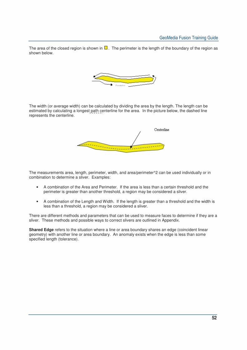
The area of the closed region is shown in . The perimeter is the length of the boundary of the region as shown below.

The width (or average width) can be calculated by dividing the area by the length. The length can be estimated by calculating a longest path centerline for the area. In the picture below, the dashed line represents the centerline.

The measurements area, length, perimeter, width, and area/perimeter^2 can be used individually or in combination to determine a sliver. Examples:

• A combination of the Area and Perimeter. If the area is less than a certain threshold and the perimeter is greater than another threshold, a region may be considered a sliver.

• A combination of the Length and Width. If the length is greater than a threshold and the width is less than a threshold, a region may be considered a sliver.

There are different methods and parameters that can be used to measure faces to determine if they are a sliver. These methods and possible ways to correct slivers are outlined in Appendix.

Shared Edge refers to the situation where a line or area boundary shares an edge (coincident linear geometry) with another line or area boundary. An anomaly exists when the edge is less than some specified length (tolerance).

��������������� �������������

53

In the above example, Line A and Area C share edge E1. The length of E1 is less than the specified tolerance; therefore, it is considered an anomaly. Line B and Area C share edge E2 whose length is greater than the specified tolerance; therefore, it is not an anomaly.

Correcting shared edge anomalies would require operator review to consider whether the features should be moved apart, their geometry edited, or left alone.

• Dead End refers to a line feature that does not terminate (both start and end) on another feature. If the length of this line feature is less than some specified tolerance, then it is considered an anomaly.

Shared Edge E1

��������������� �������������

54

Dead end anomalies may be corrected by simply removing the feature. Otherwise, operator review may be required.

������ �����������!�����������������

1. Select Toolbox > Geometric Validation > Validate Connectivity.

2. Select the Input tab and select the BuncombeCounty connection PoliticalBoundary feature class as the input feature for processing.

3. Select the Anomalies tab and check all of the Specialized anomaly options. Specify a value of 5000 as the Area in the Anomaly properties field for both slivers and gaps.

��������������� �������������

55

4. Select the OK button on the Advanced Validate Connectivity dialog.

5. Notice that 8 slivers have been detected and loaded into the Queued Edit AnomaliesQueue3 queue. The Queued Edit Map Window and Queued Edit are now activated and the anomalies are shown in the Queued Edit Map Window.

6. Add the feature class of PoliticalBoundary to the Queued Edit Map Window legend. The symbology of Political Boundary and AnomalyGeometry of Anomalies Queue2 may have to changed so the features are legible in the Queued Edit Map Window.

7. Scroll through the AnomaliesQueue2 anomaly entries and review the PoliticalBoundary feature slivers. There is currently not an option to automatically resolve sliver anomalies so it will be necessary to use GeoMedia Professional editing tools (Merge, etc.) to manually fix the slivers.

��������������� �������������

56

8. Close the Queued Edit Map Window and exit the Queued Edit command.

����#������������Attribute Validation provides a set of commands to assist you in creating attribute validation rules that can be executed against a warehouse connection that contains feature classes and attributes. The result is a validation queue of feature classes and attributes that failed during the validation of the rules, and/or a validation log file.