geomechanical testing of mrig-9 core for the potential...

SANDIA REPORT SAND2009-0852 Unlimited Release Printed February 2009

Geomechanical Testing of MRIG-9 Core for the Potential SPR Siting at the Richton Salt Dome Scott T. Broome, Stephen J. Bauer, Dennis Dunn, John H. Hofer, and David R. Bronowski Prepared by Sandia National Laboratories Albuquerque, New Mexico 87185 and Livermore, California 94550 Sandia is a multiprogram laboratory operated by Sandia Corporation, a Lockheed Martin Company, for the United States Department of Energy’s National Nuclear Security Administration under Contract DE-AC04-94AL85000. Approved for public release; further dissemination unlimited.

2

Issued by Sandia National Laboratories, operated for the United States Department of Energy by Sandia Corporation. NOTICE: This report was prepared as an account of work sponsored by an agency of the United States Government. Neither the United States Government, nor any agency thereof, nor any of their employees, nor any of their contractors, subcontractors, or their employees, make any warranty, express or implied, or assume any legal liability or responsibility for the accuracy, completeness, or usefulness of any information, apparatus, product, or process disclosed, or represent that its use would not infringe privately owned rights. Reference herein to any specific commercial product, process, or service by trade name, trademark, manufacturer, or otherwise, does not necessarily constitute or imply its endorsement, recommendation, or favoring by the United States Government, any agency thereof, or any of their contractors or subcontractors. The views and opinions expressed herein do not necessarily state or reflect those of the United States Government, any agency thereof, or any of their contractors. Printed in the United States of America. This report has been reproduced directly from the best available copy. Available to DOE and DOE contractors from U.S. Department of Energy Office of Scientific and Technical Information P.O. Box 62 Oak Ridge, TN 37831 Telephone: (865) 576-8401 Facsimile: (865) 576-5728 E-Mail: [email protected] Online ordering: http://www.osti.gov/bridge Available to the public from U.S. Department of Commerce National Technical Information Service 5285 Port Royal Rd. Springfield, VA 22161 Telephone: (800) 553-6847 Facsimile: (703) 605-6900 E-Mail: [email protected] Online order: http://www.ntis.gov/help/ordermethods.asp?loc=7-4-0#online

SAND 2009-0852 Unlimited Release

Printed February 2009

Geomechanical Testing of MRIG-9

Core for the Potential SPR Siting at the Richton Salt Dome

Scott T. Broome, Stephen J. Bauer, Dennis Dunn, John H. Hofer, and David R. Bronowski Geomechanics Department

Sandia National Laboratories P.O. Box 5800

Albuquerque, NM 87185-0751

Abstract A laboratory testing program was developed to examine the mechanical behavior of salt from the Richton salt dome. The resulting information is intended for use in design and evaluation of a proposed Strategic Petroleum Reserve storage facility in that dome. Core obtained from the drill hole MRIG-9 was obtained from the Texas Bureau of Economic Geology. Mechanical properties testing included: 1) acoustic velocity wave measurements; 2) indirect tensile strength tests; 3) unconfined compressive strength tests; 4) ambient temperature quasi-static triaxial compression tests to evaluate dilational stress states at confining pressures of 725, 1450, 2175, and 2900 psi; and 5) confined triaxial creep experiments to evaluate the time-dependent behavior of the salt at axial stress differences of 4000 psi, 3500 psi, 3000 psi, 2175 psi and 2000 psi at 55 oC and 4000 psi at 35 oC, all at a constant confining pressure of 4000 psi. All comments, inferences, discussions of the Richton characterization and analysis are caveated by the small number of tests. Additional core and testing from a deeper well located at the proposed site is planned. The Richton rock salt is generally inhomogeneous as expressed by the density and velocity measurements with depth. In fact, we treated the salt as two populations, one clean and relatively pure (> 98% halite), the other salt with abundant (at times) anhydrite. The density has been related to the insoluble content. The limited mechanical testing completed has allowed us to conclude that the dilatational criteria are distinct for the halite-rich and other salts, and that the dilation criteria are pressure dependent. The indirect tensile strengths and unconfined compressive strengths determined are consistently lower than other coastal domal salts. The steady-state-only creep model being developed suggests that Richton salt is intermediate in creep resistance when compared to other domal and bedded salts. The results of the study provide only limited information for structural modeling needed to evaluate the integrity and safety of the proposed cavern field. This study should be augmented with more extensive testing. This report documents a series of test methods, philosophies, and empirical relationships, etc., that are used to define and extend our understanding of the mechanical behavior of the Richton salt. This understanding could be used in conjunction with planned further studies or on its own for initial assessments.

3

4

Acknowledgments

The authors would like to acknowledge Brian Ehgartner and Darrell Munson, Sandia National Laboratories, for their critical review of this report.

5

Table of Contents Acronyms and Abbreviations ........................................................................................................................... 8 1 Introduction.................................................................................................................................................... 9

Background.................................................................................................................................................. 9 Technical Approach and Scope.................................................................................................................... 9

2 Salt Cores and Specimen Preparation........................................................................................................ 11 Salt Cores................................................................................................................................................... 11 Test Specimens .......................................................................................................................................... 11

3 Experimental Apparatus and Procedures ................................................................................................. 13 Mechanical Properties................................................................................................................................ 13

Acoustic Wave Velocity ........................................................................................................................ 13 Tensile Strength ..................................................................................................................................... 14 Unconfined Compressive Strength Tests ............................................................................................... 15 Quasi-static Triaxial Compression Tests................................................................................................ 15 Triaxial Compression Constant Stress Creep Tests ............................................................................... 19

Calibration ................................................................................................................................................. 21 4 Results and Analysis .................................................................................................................................... 23

Mechanical Properties................................................................................................................................ 23 Acoustic Wave Velocity Measurements ................................................................................................ 23 Density ................................................................................................................................................... 28 Indirect Tensile Strength........................................................................................................................ 31 Summary................................................................................................................................................ 33 Unconfined Compressive Strength ........................................................................................................ 34 Quasi-Static Triaxial Compression, Dilation Limit and Deformation Moduli Measurements............... 35 Creep Behavior ...................................................................................................................................... 41

5 Summary and Conclusions.......................................................................................................................... 51 6 Bibliography ................................................................................................................................................. 53 Appendix 1........................................................................................................................................................ 55 Appendix 2........................................................................................................................................................ 61 Appendix 3........................................................................................................................................................ 71

6

List of Figures Figure 1. Example of salt core cut to length using a wire saw.........................................................................12 Figure 2. Typical test setup for sonic velocity measurements..........................................................................14 Figure 3. Post test images of sample R1213 and R1203. Note vertical diametric crack..................................15 Figure 4. Testing system used to conduct quasi-static triaxial compression tests............................................17 Figure 5. Jacketed and instrumented salt specimen used in quasi-static triaxial compression testing

(pretest). ...........................................................................................................................................18 Figure 6. Sandia-designed creep testing system...............................................................................................20 Figure 7. P-wave velocity versus relative direction with 0o

arbitrary and all angles measured counter clockwise looking down on the core piece, (1) 0o, (2) 45o, (3) 90o, (4) 135o, (5) parallel to the core axis, and (6) average of all measurements..........................................................................26

Figure 8. S-wave velocity versus relative direction with 0o arbitrary and all angles measured counter

clockwise looking down on the core piece, (1) 0o, (2) 45o, (3) 90o, (4) 135o, (5) parallel to the core axis, and (6) average of all measurements..........................................................................27

Figure 9. P and S wave velocities as functions of depth for Richton salt, MRIG-9.........................................28 Figure 10. Density versus depth for Richton salt, MRIG-9. ..............................................................................29 Figure 11. Density and % Insolubles (Solids) versus depth for adjacent samples. ............................................29 Figure 12. Density versus % insolubles (Solids) for adjacent samples. .............................................................30 Figure 13. Density versus P and S wave velocity. . ..........................................................................................30 Figure 14. Indirect tensile strength versus depth................................................................................................31 Figure 15. Tensile Strength versus depth, density .............................................................................................32 Figure 16. Average indirect tensile strength for Richton salt.............................................................................33 Figure 17. Average Richton UCS compared to other rock salts. .......................................................................34 Figure 18. Dynamic elastic properties versus density........................................................................................38 Figure 19. Dilatant damage criterion of Richton salt, MRIG-9 and Big Hill salt, represented by the stress

invariants: I1 = σ1+σ2+σ3and J2 = [(σ1-σ2)2 + (σ2-σ3)2 + (σ3-σ1)2]/6. ...............................................40 Figure 20. Dilatant damage criterion of Richton salt, MRIG-9, and Big Hill salt, represented in terms of

principal stresses; axial stress at the dilation limit versus confining pressure..................................41 Figure 21. Axial strain, radial strain, and axial strain rate histories for a typical creep test of Richton

Salt, MRIG-9....................................................................................................................................43 Figure 22. Axial creep strain versus time for all Richton creep tests.................................................................44 Figure 23. Log steady-state strain rate versus log stress difference for Richton salt, MRIG-9..........................46 Figure 24. Ln steady-state strain rate versus 1/Temperature for Richton salt, MRIG-9. ...................................47 Figure 25. Predicted versus measured steady-state strain rates for Richton salt, MRIG-9. ...............................48 Figure 26. Richton creep relation versus that of other Gulf Coast domal salts. .................................................49

7

List of Tables Table 1. Summary of depth, velocity, density, and tensile strength measurements ...............................................23 Table 2. Summary of depth, velocity, density for Uniaxial and Triaxial samples. ................................................25 Table 3. Summary of quasi-static triaxial compression tests on Richton rock salt, Richton MRIG-9..................36 Table 4. Summary of static and dynamic elastic moduli determined from quasi-static triaxial compression

tests, of Richton rock salt, MRIG-9. .....................................................................................................37 Table 5. Test conditions for and results of triaxial compression creep tests on Richton rock salt, MRIG-9. .......42

Acronyms and Abbreviations

ASTM American Society for Testing and Materials RKB Rotary Kelly Bushing bgs Below ground surface Edyn, Estatic Young’s moduli, dynamic and static I1 First invariant of Cauchy stress tensor J2 Second invariant of deviatoric stress tensor LVDT Linear variable differential transformer RD Richton Dome n Creep stress exponent Q Activation energy psi Pounds per square inch R Universal gas constant T Temperature Vp, Vs Acoustic compression and shear wave velocities νdyn, νstatic Poisson’s ratio, dynamic and static

ssε& Steady-state strain rate Δσ Stress difference σ1, σ2, σ3 Principal stresses σax, σc Axial stress and confining pressure UCS Unconfined compressive strength DIVS Damage index σt Tensile strength σm Mean stress CMS Constant mean stress L Length D Diameter μ Elastic shear modulus 3-D Three-dimensional

8

9

1 Introduction

Background

The U.S. Department of Energy (DOE) is considering expanding the crude oil storage capacity of the Strategic Petroleum Reserve (SPR) to a site being considered at the Richton Salt Dome in Mississippi. The principal features of the storage facility will be a series of underground caverns. The caverns will be created by solution-mining of the natural domal salt deposit at the site. A rock salt core taken in 1982 from the Richton Salt Dome was found and examined at the Texas Bureau of Economic Geology, was determined fit to be tested, and was transported to Sandia for testing and evaluation. The locating of this core is fortuitous, as it allowed geomechanical site characterization in advance of drilling a new borehole.

Technical Approach and Scope Natural rock salt deposits are attractive materials for siting of crude oil storage caverns because they have low permeability (necessary for containment), are easily solution mined, and are located in areas of the U.S. where stored crude oil is conveniently stored for receipt and shipment to refineries. The design of caverns in salt must consider the unique mechanical behavior of the salt compared to that of other geologic media. For example, salt is known to creep (time-dependent deformation) when subjected to shear stress and elevated temperature. As a result, caverns may close over time, particularly at low cavern fluid pressures, thereby reducing the volume available for storage. In addition, salt is also known to dilate (volume expansion) through a process of stress-induced microfracturing that creates new porosity. Microfracturing may also cause localized spalling of salt slabs from the cavern roof and walls (Munson et al, 2003) which could lead to damage of the hanging strings that provide access to the stored oil and ultimately to disruption of operations. A laboratory testing program was designed within current time and budgetary constraints to begin to characterize the Richton rock salt from the available core. The characterization included primarily mechanical properties determinations and visual observations. The unique mechanical behavior characterization of Richton salt was examined using traditional mechanical properties testing of materials such as compressive and indirect tensile strength and deformation (e.g., elastic moduli), acoustic wave velocity and time dependent (creep) behavior. The approach taken in this study was that of completing some index tests (indirect tension, unconfined compressive strength) to enable us to compare the Richton rock salt with published data of other rock salts. These comparisons are presented in the results section.

10

All testing was performed on salt cores from the Richton MRIG-9 core recovered from a continuous core run from 953 ft to 1271 feet below ground surface (bgs) taken in late 1979. The salt was previously tested as part of the Office of Nuclear Waste Isolation (ONWI) program in the early/mid-1980’s that evaluated the dome as a potential candidate for high level nuclear waste storage. The tests are compiled, evaluated, and discussed by Ehgartner (2008). The report is organized as follows. Sample handling and specimen preparation are described, then experimental apparatus and procedures for mechanical testing are described followed by mechanical properties results and analysis of those results. Each data section is summarized and the data compared with existing data bases, as appropriate. Appendices provide additional detail of tests completed.

11

2 Salt Cores and Specimen Preparation

Salt Cores The salt used in the experimental study was obtained from the Richton MRIG-9 core recovered from a continuous core run from 953 ft to 1271 feet below ground surface. All depths reported are those marked on the core boxes/cores. MRIG-9 was cored approximately 500 ft into the top of salt. Thus these test results represent the salt quality near the top of the dome at this location. SPR caverns will be located from 2500 to 4500 ft deep. Additional testing of core from the new exploratory well will follow when the hole is completed. The well will be approximately 5000 ft deep.

Test Specimens Specimens used for mechanical properties testing were prepared using a two-step process resulting in cylindrical specimens with nominal diameters of 3.5 inches and length-to-diameter ratios (L:D) of approximately 2 for unconfined compression, triaxial, and creep testing. In the first step, field cores were cut to approximate length using a wire saw (Figure 1). Then in the second step, the specimens were mounted in a surface grinder where the ends of the specimens were carefully ground flat and parallel to within a tolerance of 0.001 inches following ASTM Standard D-4543 (ASTM, 1995). Samples used for tensile strength determinations were sawn to L:D ratios of 0.5; the ends of the samples were not ground. The sides of the test specimens were left undressed to avoid damage that could occur in standard machining operations. However in selecting the field cores to be processed, those cores with obvious flaws (e.g., dissolution pits, irregular or wavy surfaces) were avoided. Density was calculated from the measured mass divided by the sample volume calculated from the specimen dimensions assuming each specimen was a perfect cylinder. Because the core sat in a warehouse for an extended period of time, it was decided to “heal” all samples prior to testing to try to push grains back together at grain boundaries. This was done by jacketing samples and subjecting them to 5000 psi confining pressure and 100 oC for 24 hours. The healing process used was more rigorous than that used by others (e.g. Lee et al 2004). This process added about 4-5 hours of sample prep time to each sample. Each sample occupied the pressure vessel for 48 to 72 hours because it took on the order of 12 hours to heat and/or cool the sample-in-vessel assembly. Approximately 55 samples were prepared using this procedure; only about half of those samples were tested. About 10%-15% of samples prepared were lost to jacket leaks in the healing process. The remaining samples are available for future testing; the salt may need to be rehealed if the wait-time to testing is more than a few months. Adequacy of the healing procedure was experimentally determined by measuring the P wave velocity after successive healing times, for example 12 hours, 24 hours, 48 hours, etc.

It was found that a 24 hour healing, the healing procedure used, achieved about 90% of the P-wave velocity achieved at 4 days of healing.

Figure 1. Example of salt core cut to length using a wire saw.

12

13

3 Experimental Apparatus and Procedures

Mechanical Properties The mechanical properties testing comprised four test series: 1) acoustic compressional and shear wave velocity (Vp and Vs) measurements; 2) indirect tension tests; 3) unconfined compression tests 4) quasi-static triaxial compression tests; and 5) triaxial compression constant stress creep tests. Acoustic Wave Velocity Acoustic wave velocity measurement is a simple indirect means to identify gross mechanical differences between samples (depths) or within samples. The differences in measured values may be the result of mineralogy, grain size, or crack characteristics. Acoustic compression and shear wave velocities were measured on all of the samples, along the axis and at 45o intervals around the diameter. The diametrical directions are random, as the core was not field oriented. (Within a core section, it was assumed that the field marking of the core was consistent top to bottom; this direction was used as the zero direction, and 45o increments were measured counterclockwise looking down on the core from that scribe.) Figure 2 shows a typical setup for the velocity measurements. The apparatus consisted of a GE Panametrics 5058R unit that combined pulse generator and receiver transducers in a single package. The pulse generator and receiver transducers were attached to the salt core at positions diametrically opposed to one another. The generator produced a fast-rising, short duration electrical pulse to the transducer which induced elastic compression and shear waves into the specimen. The origin time of the wave was established by recording the electrical pulse on a Nicolet 4094 digital oscilloscope. After the wave propagated through and reached the opposite side of the specimen, the receiver converted the wave back to an electrical signal that was passed through an optional amplifier and then through a main amplifier before it was recorded by the oscilloscope. Both high and low pass filters were available to select particular band frequencies of up to 2.5 MHz. In normal operation, the scope is set to average a number of waveforms, typically 100. The average digitized signal was then stored on disk for later analysis. The analysis consisted of selecting the arrival times of the compression and shear waves knowing the origin time of the induced pulse and then calculating velocities as the ratios of the specimen diameter (or length) to the respective arrival times.

Pulse Generator & Receiver Transducers

Salt Core

Figure 2. Typical test setup for sonic velocity measurements. Tensile Strength To determine the tensile strength we used ASTM D 3967-05, Standard Test Method for determining Splitting Tensile Strength of Intact Rock Core Specimens. While direct tensile strength can be obtained by testing core in a uniaxial configuration, such a test is difficult and expensive for routine application. The splitting tensile test offers a desirable alternative. Engineers in rock mechanics design deal with complicated stress fields that include various combinations of compressive and tensile stress fields. One could argue that the tensile strength should be obtained with the presence of compressive and tensile stress conditions; the splitting tensile strength test, employed herein, is a simple test in which such stress fields occur. In this report we discuss this test as the indirect tensile strength test. In this test, typically a rock disk length/diameter = 0.5 is diametrically loaded between rigid platens (with bearing strips), until failure. See Figure 3 for a post test example of a typical sample. Table 1 lists all specimens used in the indirect tensile strength tests and includes specimen recovery depth and density. The splitting tensile strength is calculated as follows:

σt = 2P/πLD where:

σt = Splitting tensile strength (psi) P = Maximum applied load (lbs) L = Thickness of the specimen (in.) D = Diameter of the specimen (in.)

14

Figure 3. Post test images of sample R1213 and R1203. Note vertical diametric crack. As noted below, the direction chosen for tensile strength measurements is based on the velocity measurements and hopefully yields the lowest, most conservative strength.

Unconfined Compressive Strength Tests Unconfined compressive strength (UCS) tests consist of measurements of axial and lateral deformations of right circular cylinders of rock salt samples load in the axial direction to failure. The UCS test is a triaxial test with zero confining pressure and is prepared and instrumented in a manner similar to that described in the next section, “Quasi-static Triaxial Compression Tests”. The UCS is the maximum axial stress level measured at failure. Table 2 lists the specimens used in the UCS tests and also includes recovery depth and specimen density. Quasi-static Triaxial Compression Tests Strength and deformational properties of pressure-sensitive materials such as rock are commonly determined using the quasi-static triaxial compression test. In using this technique, cylindrical test specimens are initially subjected to an all-around pressure (or confining pressure) and then loaded to failure by applying compressive force to the ends of

15

16

the specimens (i.e., parallel to their central axes). The difference between the axial load (expressed in terms of stress) at failure and the confining pressure applied to the sides of the specimen is defined as the confined compressive strength. The effect of confining pressure on compressive strength is evaluated by conducting a series of tests at different confining pressures spanning the range of interest. Test specimens are normally instrumented to measure axial and radial deformations (strains) during the application of both the confining pressure (i.e., hydrostatic loading) and axial load (i.e., shear loading). The dilation stress of the sample may be determined (volume expansion of the rock salt resulting from microcracking) by examining the stress-strain measurements. Stress-strain data are also useful in evaluating particular mechanical properties such as elastic moduli. Figure 4 shows the computer-controlled servohydraulic testing system used to conduct the room-temperature (77°F) quasi-static triaxial compression tests on the Richton salt specimens described in Table 2. The system is comprised of an SBEL pressure vessel assembly and an MTS Systems reaction frame. During testing, the pressure vessel housing the test specimen was hydraulically connected to a pressure intensifier capable of inducing pressures up to 30,000 psi using Isopar® as the pressurizing medium. The reaction frame is equipped with a moveable cross-head to accommodate various sizes of pressure vessel assemblies and is capable of applying axial loads up to 1,000,000 pounds through a hydraulic actuator located in the base of the frame. Vessel pressures were measured by a pressure transducer plumbed directly into the hard line that supplies the pressure to the vessel. It is located ~ 10 ft. from the vessel pressure. Axial loads were measured by a load cell located outside the pressure vessel. Each test specimen was jacketed in a ~1/16-inch-thick impervious heat shrink membrane to prevent the confining pressure fluid from contacting and/or entering the pore space of the specimen when it was placed under pressure in the pressure vessel. The jackets were sealed to hardened steel end caps above and below the specimen with 304 stainless steel wire. The ends of the specimens are lubricated to the end caps with a 50:50 mixture of Vaseline and stearic acid. Test specimens were instrumented with electronic deformation transducers before they were placed in the pressure vessel assembly. Radial deformation was measured using a chain gage which wrapped around the circumference of the sample at midheight. As shown in Figure 5, the chain gage provides an average circumferential strain measure. Axial deformation was measured by linear variable differential transformers (LVDTs) mounted to the specimen endcaps.

Figure 4. Testing system used to conduct quasi-static triaxial compression tests.

17

18

Figure 5. Jacketed and instrumented salt specimen used in quasi-static triaxial compression testing (pretest). Setup of the quasi-static triaxial compression tests included placing the jacketed, instrumented specimen assembly into the pressure vessel, connecting instrumentation leads to feed-throughs in the pressure vessel and mounting the pressure vessel assembly into the reaction frame (see Figure 4). The actuator in the base of the frame was then advanced gradually raising the pressure vessel assembly into position for the test. A small axial preload was applied to the specimen through a push-rod that extended through the top of the pressure vessel and was in direct contact with the crosshead load cell on one end and the specimen on the other. Then, initiation of the test was turned over to the test system controllers which automatically increased the confining pressure and axial stress to ensure the specimen was loaded to the correct hydrostatic confining stress. Once the test system had stabilized at the target pressure, additional axial load was applied to the specimen until

19

the test was terminated either because a peak axial load was reached or the range of the deformation transducers had been exceeded. Axial loading was interrupted several times during each test to initiate an unload/reload cycle. As discussed, the unload/reload stress-strain data were used to evaluate static elastic moduli. Triaxial Compression Constant Stress Creep Tests The time-dependent deformational behavior of Richton salt was determined through a series of triaxial compression constant stress creep tests. These tests are similar to the quasi-static triaxial compression tests in that the specimen is initially subjected to an all-around confining pressure. Then however, a constant axial stress difference (axial stress minus confining pressure), less than or equal to the confining stress, is applied to the specimen and deformations are measured as a function of time. Creep deformation of salt is highly dependent both on the magnitude of the applied stress difference and the temperature at which the test is conducted. Therefore, a series of tests is usually performed at different stresses and temperatures to evaluate the effects of these variables on creep. Figure 6 shows a typical Sandia-designed creep testing system. It consists of a load frame that reacts against the axial forces applied by the hydraulic cylinder located at the base of the frame and the pressure vessel that houses test specimens during testing. The hydraulic cylinder and load frame are capable, respectively, of applying and reacting axial loads of up to 350,000 pounds. The pressure vessel is rated to 10,000 psi and is equipped with electrical band heaters capable of maintaining test temperatures up to 150°C (~300°F). Silicon oil is used as the pressurizing medium. Fluid pressures are adjusted using an air-assisted pump and can be maintained constant using a dilatometer system that either injects or withdraws oil from the vessel. Vessel pressures are measured by a pressure transducer plumbed into the hydraulic line leading from the vessel to the dilatometer. Axial loads applied by the hydraulic cylinder are measured by a load cell located directly above the cylinder in line with the axial push-rod that extends into the pressure vessel and applies axial load to the ends of the specimen. Test temperature is recorded by two thermocouples, one located near the top of the pressure vessel and other near the vessel midheight. As with the quasi-static triaxial compression tests, each specimen is placed between two metal endcaps and jacketed to protect it from the pressurizing fluid. For the creep tests, the specimens were jacketed with flexible Viton tubing (rather than shrink tubing) that was secured to the endcaps with 304 stainless lock wire (Vaseline/stearic acid is again used as the end lubricant). The specimen assembly was placed inside the pressure vessel, which was then filled with silicon oil. The pressure in the vessel was increased to the target level (4,000 psi for all the creep tests in this study) and allowed to stabilize. The vessel was then heated to the target temperature by activating the band heaters located on the outside of the pressure vessel. The temperature was allowed to stabilize for approximately 24 hours. After this stabilization period was completed, the target stress difference was applied by rapidly increasing the axial load on the specimen using the hydraulic cylinder. When the target load was reached, control of the test was turned over to an Azonics controller that maintained the axial stress constant throughout the duration of the test and also served as the

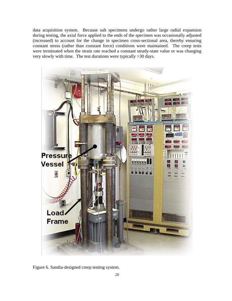
data acquisition system. Because salt specimens undergo rather large radial expansion during testing, the axial force applied to the ends of the specimen was occasionally adjusted (increased) to account for the change in specimen cross-sectional area, thereby ensuring constant stress (rather than constant force) conditions were maintained. The creep tests were terminated when the strain rate reached a constant steady-state value or was changing very slowly with time. The test durations were typically >30 days.

Figure 6. Sandia-designed creep testing system.

20

21

Creep deformations were measured by electronic transducers mounted outside the pressure vessel in contrast to the on-the-specimen method used in the quasi-static triaxial compression tests. Axial deformation was measured by two LVDTs that tracked the displacement of the axial push-rod relative to the bottom of the pressure vessel. This displacement was a direct measure of the axial displacement of the specimen because non-specimen deformations were negligible given the imposed constant stress condition. The LVDTs were mounted 180º apart on the push-rod. The calibrated ranges of the LVDTs were either 0.05 or 0.1 inches and 1 inch allowing accurate measurements of both small and relatively large strains. During the tests, the 0.05 or 0.1-inch-range LVDTs were reset periodically when the range was exceeded. Radial deformations were measured indirectly by measuring the volume of oil that was either injected into or removed from the vessel by the dilatometer system with an appropriate correction for the volume displaced by the push-rod as it moved into or out of the pressure vessel. This technique, developed by Wawersik (1979), is accurate to within 2% provided constant pressure and temperature conditions are maintained and the confining system is leak free.

Calibration Data collected in the experimental study included force, pressure, temperature, displacement, and volume change. Typically, these data are acquired using electronic transducers in which the electrical output is proportional to the change in the measured variable. In all cases, the constants of proportionality were determined through careful calibration using standards traceable to the National Institute for Standards and Technology. In the case of the creep tests, all data were measured as a function of time.

23

4 Results and Analysis

Mechanical Properties Acoustic Wave Velocity Measurements P (compressional) and S (shear) wave velocities were measured for all specimens prepared for tensile strength, uniaxial, and triaxial testing. The purpose of the velocity measurements was to assess the homogeneity of each rock salt sample and the homogeneity of the rock salt along the core length. The tensile strength samples were evaluated in a multi-directional manner, specifically to determine fast or slow velocity directions (indications of inhomogeneity or anisotropy). Also, it is hypothesized that a slow velocity direction may indicate alignment of cracks or flaws in the rock salt. Measurement of tensile strength perpendicular to this slow velocity direction would measure the weakest (most conservative) tensile strength (if this hypothesis is correct). Twelve specimens were examined for the depths indicated in Table 1, which summarizes all velocity and density measurements on the indirect tension test samples. Similar information for unconfined compressive strength and triaxial specimens is presented in Table 2.

Table 1. Summary of depth, velocity, density, and tensile strength measurements

Sample/depth (ft) Pt / angle P velocity

Km / s S velocity

Km / s Density

g/cc Indirect Tensile Strength (psi)

R1040BZ/1040 1 / 0º 3.837 2.419 Anhydrite & Halite 2 / 45° 4.199 2.696 3 / 90° 4.166 2.578 2.11 220 4 / 135° 4.547 2.558

5 / axial 4.640 2.528

average 4.278 2.556 R1062BZ/1062 1 / 0º 4.502 2.639 2.20 200 Anhydrite & Halite 2 / 45° 4.515 2.638 3 / 90° 4.392 2.601 4 / 135° 4.416 2.689 5 / axial 4.652 2.774

average 4.495 2.668

R1100BZ/1100 1 / 0º 4.540 3.031 Halite 2 / 45° 4.529 2.619 3 / 90° 4.576 2.571 4 / 135° 4.563 2.605 2.17 250 5 / axial 4.612 2.881 average 4.564 2.741

24

Table 1. Summary of depth, velocity, density, and tensile strength measurements

R1105BZ/1105 1 / 0º 4.340 2.756 Halite 2 / 45° 4.370 2.561 3 / 90° 4.380 2.646 2.17 185 4 / 135° 4.533 2.975 5 / axial 4.484 3.016 average 4.421 2.791 R1168BZ/1168 1 / 0º 4.456 2.518 Anhydrite & Halite 2 / 45° 4.235 2.508 3 / 90° 4.405 2.533 4 / 135° 4.540 3.416 2.18 200 5 / axial 4.393 3.443 average 4.406 2.884 R1197BZ/1197 1 / 0º 4.498 2.600 2.20 200 Anhydrite & Halite 2 / 45° 4.560 2.555 3 / 90° 4.439 2.572 4 / 135° 4.682 2.611 5 / axial 4.639 3.399

average 4.564 2.748

R1203BZ/1203 1 / 0º 4.549 2.734 2.19 250 Halite 2 / 45° 4.629 2.622 3 / 90° 4.109 2.605 4 / 135° 4.497 2.285 5 / axial 4.715 2.677

average 4.500 2.585

Sample/depth (ft) Pt / angle P velocity

Km / s S velocity

Km / s Density

g/cc Indirect Tensile Strength (psi)

R1213BZ/1213 1 / 0º 4.148 2.533 Anhydrite & Halite 2 / 45° 4.535 2.552 3 / 90° 4.496 2.575 2.16 170 4 / 135° 4.287 2.442 5 / axial 4.560 3.075 average 4.405 2.635 R1230BZ/1230 1 / 0º 4.159 2.304 Halite 2 / 45° 4.210 2.586 3 / 90° 4.300 2.610 2.16 175 4 / 135° 4.474 2.784 5 / axial 4.419 2.545 average 4.312 2.566 R1237BZ/1237 1 / 0º 4.474 2.545 Anhydrite & Halite 2 / 45° 4.292 2.619 3 / 90° 4.435 2.629 4 / 135° 4.469 2.586 2.16 170 5 / axial 4.683 3.671 average 4.471 2.810 R1248BZ/1248 1 / 0º 4.431 2.640

25

Table 1. Summary of depth, velocity, density, and tensile strength measurements Halite 2 / 45° 4.494 2.584 2.16 150 3 / 90° 4.368 2.650 4 / 135° 4.343 2.522 5 / axial 4.458 2.368 average 4.419 2.553 R1263BZ/1263 1 / 0º 4.397 2.660 Halite 2 / 45° 4.365 2.616 2.17 200 3 / 90° 4.259 2.069

4 / 135° 4.117 2.415 5 / axial 4.536 3.306 average 4.335 2.613 Green highlight indicates direction of test; dimensions for strength calculation

Note: Anhydrite & Halite and Halite designations were made by visual inspection during the viewing of the core at the Texas Bureau of Economic Geology in early 2008. The velocities shown in bold represent the minimum velocities measured.

Table 2. Summary of depth, velocity, density for Uniaxial and Triaxial samples.

Sample ID Test ID Lithology Depth P-wave velocity Density

ft km/s g/cc R1198 Richton-TA01 Halite & anhydrite 1198 4.204 2.23

R1165B Richton-TA02 Halite & anhydrite 1165 4.104 2.18 R1039 Richton-TA03 Halite & Anhydrite 1039 4.595 2.20 R1222 Richton-TA04 Halite & Anhydrite 1222 4.101 2.18 R1197 Richton-TA05 Halite & Anhydrite 1197 4.542 2.19 R1141 Richton-TA06 Halite 1141 3.961 2.15 R1100 Richton-TA07 Halite 1100 4.111 2.17 R1081 Richton-TA08 Halite 1081 4.464 2.20

R1105B Richton-TA09 Halite 1105 4.381 2.16

R1245 Richton-UC01 Halite 1245 3.864 2.16 R1166 Richton-UC02 Anhydrite & Halite 1166 4.517 2.18 R1246 Richton-UC03 Halite 1246 4.552 2.16 R1163 Richton-UC04 Halite & Anhydrite 1163 4.515 2.17 R1040 Richton-UC05 Halite & Anhydrite 1040 4.599 2.22 R1265 Richton-UC06 Halite & Anhydrite 1265 3.412 2.21

Figures 7 and 8 display, respectively, the P and S wave velocity versus direction in each sample. The 00 measurement direction is arbitrary for each piece of core. Within the core the variation in P and S wave velocities of about 0.5 km/s or more is measurable with a few

exceptions, indicating the samples are not isotropic and/or the samples are not fully healed. The minimum P wave velocity direction in each sample was noted, and because a low P wave velocity may denote a direction with more cracks perpendicular to it, we chose to measure the tensile strength perpendicular to that direction, in an attempt to measure the “lowest” strength.

P-Wave Velocity- Indirect Tension Samples

3.8

3.9

4

4.1

4.24.3

4.4

4.5

4.6

4.7

4.8

0 1 2 3 4 5 6 7

Relative Measurement Direction

P-W

ave

Vel

ocity

(Km

/s) R1040

R1062R1100R1105R1168R1197R1203R1213R1230R1237R1248R1263

Figure 7. P-wave velocity versus relative direction with 0o

arbitrary and all angles measured counter clockwise looking down on the core piece, (1) 0o, (2) 45o, (3) 90o, (4) 135o, (5) parallel to the core axis, and (6) average of all measurements.

26

S-Wave Velocity- Indirect Tension Samples

2

2.2

2.4

2.6

2.83

3.2

3.4

3.6

3.8

4

0 1 2 3 4 5 6 7

Relative Measurement Direction

S-W

ave

Vel

ocity

(Km

/s) R1040

R1062R1100R1105R1168R1197R1203R1213R1230R1237R1248R1263

Figure 8. S-wave velocity versus relative direction with 0o

arbitrary and all angles measured counter clockwise looking down on the core piece, (1) 0o, (2) 45o, (3) 90o, (4) 135o, (5) parallel to the core axis, and (6) average of all measurements. Figure 9 plots the average P and S wave velocity measurements as a function of depth. The variability in both P and S wave velocity is about 0.5 km/s with depth. The P and S wave velocities average about 4.4 km/s and 2.6 km/s, respectively. The variability and spread of the P and S wave velocity indicates that the rock salt is inhomogeneous (by its composition or amount of healing, or both) at each depth sampled and that inhomogeneity persists within this depth interval.

27

Tension and Triaxial Samples Average Velocity vs Depth1000

1050

1100

1150

1200

1250

13002.1 2.6 3.1 3.6 4.1 4.6

Velocity (km/s)

Dep

th (f

t)P Velocity TensionS Velocity TensionP Velocity Triaxial S Velocity Triaxial

Figure 9. P and S wave velocities as functions of depth for Richton salt, MRIG-9. Density Density was determined by the specimen mass divided by its volume. The specimen volume was determined by measuring the specimen length and diameter and calculating the volume assuming the specimen was a right circular cylinder. Figure 10 plots specimen depth versus density. The density range (about 5%) is indicative of the rock salt mass inhomogeneity within this depth interval. We attempt to relate density to mineralogy through the visual relationships in Figure 11 and plotted in Figure 12. In samples which were immediately adjacent to the sample used for mechanical testing we measured density and then we dissolved away the solubles, leaving behind insolubles, which are predominantly anhydrite by visual identification. We observe associations of density and insoluble content; the greater the insoluble content, the greater the density. There appears to be a correlation between P- and S-wave velocity and density (Figure 13). This is consistent with theory. The relationship is better for P-wave velocity.

28

Density vs Depth1000

1050

1100

1150

1200

1250

13002.1 2.12 2.14 2.16 2.18 2.2 2.22 2.24

Density (g/cc)

Dep

th (f

t)

Indirect TensionTriax Samples

Figure 10. Density versus depth for Richton salt, MRIG-9.

1050

1100

1150

1200

1250

1300

0 2 4 6 8 10 12

% Solids

Dep

th (f

t)

2.15 2.16 2.17 2.18 2.19 2.2 2.21

Density (g/cc)

% SolidsDensity

Figure 11. Density and % Insolubles (Solids) versus depth for adjacent samples.

29

Density vs % Solids

y = 150.82x - 325.04

0

2

4

6

8

10

12

2.15 2.16 2.17 2.18 2.19 2.2 2.21

Density

% S

olid

s

Series1

Linear (Series1)

Figure 12. Density versus % insolubles (Solids) for adjacent samples.

Average Velocity versus Density

y = 0.6401x + 1.2335

y = 2.0417x - 0.0499

2

2.5

3

3.5

4

4.5

5

2.1 2.12 2.14 2.16 2.18 2.2

Density (g/cc)

Velo

city

(Km

/s)

P Velocity tensionS Velocity tensionP velocity triaxialS Velocity triaxialLinear (S wave all)Linear (P wave all)

Figure 13. Density versus P and S wave velocity. The data plotted are average from triaxial samples and indirect tension samples. For the equations, y = velocity, x = density.

30

Indirect Tensile Strength Indirect tensile strength of a specimen listed together with the direction of lowest velocity is given in Table 1. Tensile strength values versus depth are given in Figure 14. The range in strengths for all the data is large but not atypical of this type of index test measurement, with this number of tests. There is no apparent depth versus indirect tensile strength relationship, and we did not anticipate such a relationship. Rather the tensile strength is probably better related to the mineralogy, texture, crack structure, etc. The data base is too small to make such correlations, however, in Figure 15 we replot the tensile strength versus depth data along with the tensile strength versus density data. Indeed there does not appear to be a viable relationship between tensile strength and density.

Indirect Tensile Strength vs Depth1000

1050

1100

1150

1200

1250

1300150 170 190 210 230 250

Indirect Tensile Strength (psi)

Dep

th (f

t)

Figure 14. Indirect tensile strength versus depth.

31

Figure 15. Tensile Strength versus depth, density In Figure 16, the Richton average strength (Site 1) suggests a strength slightly below the average strength (red line) of seventeen other salt sites (individual data points).

32

Richton Salt Indirect Tension Compared to Other Sites

150

180

210

240

270

300

0 1 2 3 4 5 6 7 8 9 10 11 12 13 14 15 16 17 18 19

Site

Indi

rect

Ten

sile

Str

engt

h (p

si)

Figure 16. Average indirect tensile strength for Richton salt (Richton data is Site 1, average of 12 measurements), average indirect tensile strengths for 17 other salts from around the world (individual data points), and average of all data (red line). Summary Results of acoustic velocity (P and S wave) measurements, indirect tension tests, density determinations of those samples, their sample to sample variations, averages and their inter-relationships were presented. Velocity data show variability; this variability is greater than that observed for other domal salts. This variation is likely of two sources: (1) The samples sat for many years, and were allowed to relax and disassociate at grain boundaries. We attempted to heal the samples—perhaps this healing was incomplete. If the healing was only slightly incomplete, the velocity would have been significantly effected. This incomplete healing could be the source of at least some of the velocity variation observed (Velocities are very sensitive to cracks). (2) The density and mineralogic differences provided intrinsic differences from sample to sample. Perhaps, for these samples, velocity measurements do not provide a valuable discriminator, as compared with our experience with other salts. Perhaps this judgment will be born out with future measurements and testing. The indirect tensile strength of these twelve samples is also spread out, and on the average, plots low when compared to other domal salts.

33

Unconfined Compressive Strength Summary The unconfined compressive strength (UCS) of Richton rock salt was determined by standard compression tests of right circular cylinders. The UCS values are listed in Table 3; stress strain data for these tests are presented in Appendix 1. The average UCS for the Richton salt is below average with respect to other salts. Richton rock salt UCS compared to other rock salts The average UCS (4 measurements) for the Richton rock salt (Site 1) is compared to other salts in Figure 17. The Richton salt average strength (Site 1) is less than the average of the rock salts (red line) in this compilation.

Figure 17. Average Richton UCS compared to other rock salts. (Richton data is Site 1, average of 4 measurements).

34

Quasi-Static Triaxial Compression, Dilation Limit and Deformation Moduli Measurements Nine quasi-static triaxial compression tests were performed on rock salt cores from the cavern horizon to determine the dilational compressive strengths and static elastic properties. Table 3 summarizes certain key results for the quasistatic testing. Appendix 2 provides the stress difference versus axial, lateral and volumetric strains for each of the nine triaxial tests. The dilation stress was defined as the stress difference corresponding to the shift from positive to negative volume strain in the stress difference versus volumetric strain curve. The convention is that dimensional decreases are positive and volume decreases are positive; dimensional increases are negative and volume increases are negative.

Static Elastic Moduli: Static elastic moduli determined from the unload/reload data acquired during the quasi-static triaxial compression tests are summarized in Table 4. The static elastic Young’s modulus, Estatic, was determined directly from the slope of the unload/reload stress difference versus axial strain curve. Values of static elastic Poisson’s ratio, were calculated from the ratio of Estatic to the slope of the unload/reload stress difference versus lateral strain curve. Young’s modulus ranges from approximately 4.0 × 106 psi to 5.2 × 106 psi for Triaxial tests. Poisson’s ratio ranges from approximately 0.08 to 0.17. Dynamic Elastic Moduli: Dynamic elastic moduli determined from the P and S wave velocity measurements, together with the density measurements on those samples are summarized in Table 4. The dynamic elastic Young’s modulus, Edynamic, was determined directly from:

( )( )VV

VVVSP

SPSdynamicE 22

222 43−

−=

ρ

Values of dynamic elastic Poisson’s ratio, were calculated from:

( )( )VV

VVSP

SPsRatioPoisson 22

22

2

2'

−

−=

Dynamic Young’s modulus ranges from approximately 4.4 × 106 psi to 6.1 × 106 psi for triaxial test samples. Poisson’s ratio ranges from approximately 0.19 to 0.29. Dynamic elastic properties may be correlated with dynamic properties determined from geophysical well log measurements. There appears to be a relationship (albeit weak) between dynamic elastic properties and density (Figure 18).

35

36

Table 3. Summary of quasi-static triaxial compression tests on Richton rock salt, Richton MRIG-9.

Test no. Test type

Depth middle

Confining pressure,

P (σ3 initial)

Unconfined Compressive

Strength, (UCS) σdiff σ1,d

σ3,d I1,d J20.5

,d

(ft) (psi) (psi) (psi) (psi)

(psi) (psi) (psi) Richton-TA01 Triaxial 1198 725 3237 3963 726 5415 1869 Richton-TA02 Triaxial 1165 1450

2987 4441 1454 7349 1725.

Richton-TA03 Triaxial 1039 2150

2871 5047 2177 9401 1657


2494 5398 2903 11204 1440


2679 3405 726 4857 1547


2638 3365 727 4819 1523


3712 5165 1453 8071 2143


4194 6370 2176 10722 2421


4127 7030 2903 12836 2383

Richton-UC01 UCS 1245 0 2324 984 984 0 984 568 Richton-UC02 UCS 1166 0 2845 1456 1456 0 1456 841 Richton-UC031 UCS 1246 0 1275 1042 1042 0 1042 602 Richton-UC041 UCS 1163 0 1423 1289 1289 0 1289 744 Richton-UC05 UCS 1040 0 2497 1741 1741 0 1741 1005 Richton-UC06 UCS 1265 0 2334 1768 1768 0 1768 1020 1 These samples are believed defective because a contact media was used for the velocity measurements, then the samples were healed; it is believed that the contact media permeated throughout the samples during healing, reducing the strength. This data was not used in any analyses. I1 – First invariant of the stress tensor; J2 – Second invariant of the deviatoric stress tensor d – at dilation; σdiff – differential stress at dilatation

37

Table 4. Summary of static and dynamic elastic moduli determined from quasi-static triaxial compression tests, of Richton rock salt, MRIG-9.

Triaxial tests Reload # Modulus (psi) Poisson's Ratio

Dynamic Modulus

(psi)

Dynamic Poisson's

Ratio

Richton-TA01 None

4.494E+06

0.23

Richton-TA02 1 4.482E+06 0.078

6.07E+06

0.19 2 4.421E+06 0.137 3 4.177E+06 0.113

Richton-TA03 1 4.552E+06 0.069

5.54E+06

0.26 2 4.493E+06 0.086 3 4.274E+06 0.114

Richton-TA04 1 4.472E+06 0.091

4.68E+06

0.17 2 4.304E+06 0.103 3 4.325E+06 0.093

Richton-TA05 1 5.199E+06 0.107

5.44E+06

0.25 2 4.564E+06 0.092 3 4.154E+06 0.079

Richton-TA06 1 4.090E+06 0.110

4.90E+06

0.19 2 4.041E+06 0.087 3 3.645E+06 0.173

Richton-TA07 1 4.319E+06 0.094

4.45E+06

0.25 2 4.451E+06 0.110 3 3.999E+06 0.139

Richton-TA08 1 4.477E+06 0.094

5.37E+06

0.25 2 4.256E+06 0.110 3 4.155E+06 0.136

Richton-TA09 1 4.323E+06 0.128

4.64E+06

0.29 2 4.207E+06 0.106 3 4.005E+06 0.131

Average 4.308E+06 0.1074

5.07E+06*

0.21* Shear modulus

(psi): 1.945E+06

*This average includes data from tensile strength samples.

Figure 18. Dynamic elastic properties versus density.

Dilatational Strength: The onset of dilatant damage can be defined in several ways. However, for consistency with the literature (Mellegard and Pfeifle, 1994), it will be defined as the point at which the rock reaches its minimum volume (or dilation limit). In this work, the onset of dilatancy is chosen as the onset of the negative trend in volumetric strain from the stress strain data collected. Table 3 summarizes the results from our laboratory experimental program of Richton salt consisting of nine triaxial compression tests and six uniaxial compression tests with zero confining pressure.

The stress states that produce failure and/or dilation of pressure-dependent materials are often expressed in terms of two stress invariants, i.e., the first invariant of the Cauchy stress tensor, I1, and the second invariant of the deviatoric stress tensor, J2. These two invariants are defined mathematically as:

3211 σσσ ++=I Eq. 1

( ) ( ) ({ }213

232

2212 6

1 σσσσσσ −+−+−=J ) Eq. 2

38

39

where σ1, σ2, and σ3 are the maximum, intermediate, and minimum principal stresses, respectively. The experimental dilational strengths are also plotted in Figures 19 and 20. In Figure 19, we present the Richton dilational strength data, plotted in I1 versus root J2 space and in Figure 20, we present the Richton dilational strength data, plotted in confining pressure versus σ1 at dilation along with data from another SPR site salt, Big Hill (Lee et al, 2004). The Richton data is separated into Halite, and Anhydrite and Halite groupings. For each of the three “rock salts” represented, there appears to be distinct pressure dependencies of the dilational strength represented. Secondly, Richton salt types high in halite content and lower in halite content clearly show a distinction in the strength data, with the higher halite content salt being stronger. This observation should be better enumerated with further testing. The weaker of the two Richton salts is comparable in strength to the Big Hill salt.

Figure 19. Dilatant damage criterion of Richton salt, MRIG-9 and Big Hill salt, represented by the stress invariants: I1 = σ1+σ2+σ3 and J2 = [(σ1-σ2)2 + (σ2-σ3)2 + (σ3-σ1)2]/6. The data and equations are color coded as follows, Blue: Richton salt; Halite rich rock, Black: Richton salt; Anhydrite and Halite rock, Red: Big Hill salt.

40

Confining Pressure vs Sigma 1 at Dilatation Stress State

y = 1.4253x + 1904.5

y = 2.1714x + 1367.4

y = 1.2511x + 2248.2

0500

10001500200025003000350040004500500055006000650070007500

0 500 1000 1500 2000 2500 3000 3500 4000

Confining Pressure (psi)

Sigm

a 1

at D

ilatio

n

Anhydrite & HaliteHaliteBHLinear (Anhydrite & Halite)Linear (Halite)Linear (BH)

Figure 20. Dilatant damage criterion of Richton salt, MRIG-9, and Big Hill salt, represented in terms of principal stresses; axial stress at the dilation limit versus confining pressure. The data and equations are color coded as follows, Blue: Richton salt; Halite rich rock, Black: Richton salt; Anhydrite and Halite rock, Red: Big Hill salt. For the equations, y= Sigma 1 at Dilation, and x = Confining Pressure.

Creep Behavior A total of seven creep tests were performed on Richton salt. Only salt high in halite content was tested. All tests except one were conducted at a confining pressure of 4,000 psi and at stress differences ranging from 2,000 to 4,000 psi. (see Table 5). The 4,000 psi confining pressure tests were conducted at 55°C, except for one that was tested at 35°C. The conditions were chosen as representative of those at the cavern quarter height.

41

42

Table 5. Test conditions for and results of triaxial compression creep tests on Richton rock salt, MRIG-9.

Test I.D.

Recovery Depth (feet)

Stress Difference

(psi)

Temperature (°C/°F)

Test Duration

(days)

Final Axial Strain Rate measured

(s-1)

Final Axial Strain Rate calculated

(s-1)

A2 #1 1109 2175 52 52 3.22E-09 N/A

A1 #1 1126 3000 55 38 1.71E-08 1.53E-08 A3 #1 1262 4000 55 14 7.68E-08 7.59E-08 A3 #2 1127.5 3500 55 30 2.33E-08 3.61E-08 A3 #3 1145 2000 55 36 1.38E-09 1.61E-09 A1 #2 1142.8 3000 55 44 1.68E-08 1.53E-08

A2 #2 1144 4000 35 35 2.87E-08 2.84E-08

Confining pressure = 4000 psi in all tests except A2 #1 (1450 psi). Figure 21 plots axial, radial, and volumetric strains versus time and axial strain rate versus time for a typical creep test on Richton salt. The two axial strain curves represent the output from two independent measurements of axial deformation – one using a lower range LVDT (0 to 0.05 inches) and other using a higher range LVDT (0 to 1.0 inches). Both the axial and radial strain curves are typical of rock salt in that the strain rates are high initially but then decrease monotonically to a constant or nearly constant value over time. In this example, the strain rate reaches a constant value (~2.33×10-8 s-1) between 24 and 29 days. Similar plots are provided in Appendix 3 for each of the seven creep tests. Plots of stress difference, confining pressure, and temperature are also shown in Appendix 3 for each test. Axial strain for each of the seven creep tests is plotted in Figure 22. The respective curves are well ordered in that the smallest strains are seen for the lowest stress difference magnitudes. Also, the single test performed at 35°C fits well because its strain curve is below the 55°C test with the same parameters. The experimental value for axial strain rate was calculated from the slope of the axial strain vs. time data using the linear-least squares method. Approximately the last five days of axial strain data were used from each creep test to determine the measured axial strain rate with the exception of test A1#1. Test A1#1 was accidentally overloaded multiple times due to the axial load increasing beyond the required 4000 psi stress difference. This can be seen in the plot of test A1#1 in Figure 22. The steady state rate for this test was calculated from a 24 hour period prior to the final overload at ~ 27 days. A duplicate test was run (A1#2) in order to check that the data for test A1#1 was reliable. In this section we discuss creep experiments and derivation of a creep expression for the Richton rock salt. Sophisticated mathematics and fitting procedures are used in deriving the empirical parameters in the creep expression. The small number of tests performed limits our judgment of the creep expression to an estimate.

-0.1

-0.05

0

0.05

0.1

0.15

0 5 10 15 20 25 30 35

Time (days)

Stra

in

1.00E-08

1.00E-07

1.00E-06

Axi

al S

trai

n R

ate

(1/s

ec)

Axial Strain (1-in LVDT)

Axial Strain (0.05-in LVDT)Radial Strain

Volumetric Strain

Strain rate

Richton SaltTest A3#2 Δσ = 3500 psi σ3 = 4000 psi T = 55 C

2.33E-8

Figure 21. Axial strain, radial strain, and axial strain rate histories for a typical creep test of Richton Salt, MRIG-9.

43

0

0.02

0.04

0.06

0.08

0.1

0.12

0.14

0.16

0.18

0.2

0 10 20 30 40 50 60

Time (days)

Axi

al c

reep

str

ain

A1#1(3000psi,55deg) A1#2(3000psi,55deg)

A2#1(2175psi,52deg) A2#2(4000psi,35deg)

A3#1(4000psi,55deg) A3#2(3500psi,55deg)

A3#3(2000psi,55deg)

Richton SaltConfining pressure=4000 psi except test A2#1 confining pressure=1450 psi

Figure 22. Axial creep strain versus time for all Richton creep tests. Strain curve for test A1#1 exhibits overload spikes due to brief loss of axial load control during testing. Steady-State Strain Rate Analysis The creep behavior of salt is often characterized using a steady-state only creep law represented by the following equation:

⎟⎠⎞

⎜⎝⎛−⎟⎟

⎠

⎞⎜⎜⎝

⎛ Δ=

RTQA

n

ss expμσε& Eq 3

where ssε& is the steady-state creep rate, Δσ is the stress difference, μ is the elastic shear modulus for salt, T is temperature (expressed in °K where °K=°C+273), R is the Universal gas constant (1.99 cal/mole°K), and A, n and Q are model parameters. The parameters n and Q are also known as the stress exponent and activation energy, respectively. The model parameters can be determined by fitting Equation 3 to steady-state strain rate data collected at different stress differences and temperatures. The nonlinear form of Equation 3 requires nonlinear fitting routines, which are readily available from numerous statistical software packages; however, Equation 3 can be transformed into linear space by making a few simple assumptions. For example, if all testing is performed at a constant temperature, as in most of the Richton test series, Equation 3 can be re-written as:

44

n

ss A ⎟⎟⎠

⎞⎜⎜⎝

⎛ Δ′=μσε& Eq 4

where A′ is a new parameter that incorporates A and the temperature term of Equation 3. Equation 4 can then be linearized through a logarithmic transformation to yield

( ) ⎟⎟⎠

⎞⎜⎜⎝

⎛ Δ+′=

μσε log)log(log nAss& Eq 5

Plotting steady-state strain rate and stress difference in this transformed space will result in a straight line with a slope of n. Constant temperature data given in Table 5 (T=55°C) was transformed as defined in Equation 5 and then plotted in the respective transformed space as shown in Figure 23. The data in these plots were fitted using linear-least squares to determine estimates of n. Based on the constant temperatures of 328°K, the value of n was determined to be 5.56. A value of n = 5 is typical of many salts (e.g., Munson et al, 1988). Two tests were performed at a constant stress difference at different temperatures. Plotting data with these parameters can be done by re-writing Equation 3 as:

⎟⎠⎞

⎜⎝⎛−=

•

RTQAss exp"ε Eq 6

where A” is yet another parameter that incorporates A and the stress term of Equation 3. Equation 6 can be linearized through a natural logarithmic transformation to yield:

( )TR

QAss1lnln " ⋅−=⎟

⎠⎞

⎜⎝⎛ •

ε Eq 7

Plotting the natural logarithm of steady-state strain rate against inverse of temperature results in another straight line with a slope of Q/R as shown in Figure 24. The value of Q/R was found to be -4977 or a Q value of 9954 cal/mol. Values of Q = 10000 cal/mol are often reported for salt (Wawersik, 1992). The values of n and Q determined from the linear transformations served as constants for a nonlinear fitting process used to evaluate the model parameter A in Equation 3 directly. This fitting process made use of the commercially-available SOLVER routine included with Microsoft Excel® to yield the following best fit steady-state creep model for Richton salt:

⎟⎠⎞

⎜⎝⎛−⎟⎟

⎠

⎞⎜⎜⎝

⎛ Δ×=

•

RTss

9954exp10592.256.5

14

μσε Eq 8

45

All of the steady-state data given in Table 5 was used in the nonlinear fit resulting in the parameter estimate of A shown in Equation 8. Equation 8 was used to predict the steady-state strain rates given in Table 5. These predictions or calculated steady-state rates are shown in Figure 25 and are in good agreement with the measured data. In Figure 26 we compare the creep expression estimate from this study to that of other rock salts; the Richton rock salt creeps at an intermediate rate.

y = 5.5628x - 27.19

-9.5

-9.0

-8.5

-8.0

-7.5

-7.0

-6.5

3.2 3.25 3.3 3.35 3.4 3.45 3.5 3.55 3.6 3.65 3.7

Log(Stress Difference) - psi

Log(

Stra

in R

ate)

- 1/

sec

Temp. ~ 328 K

Temp. ~ 308 K

1

n=5.56

Figure 23. Log steady-state strain rate versus log stress difference for Richton salt, MRIG-9.

46

y = -4976.6x - 1.2163

-18.0

-17.8

-17.6

-17.4

-17.2

-17.0

-16.8

-16.6

-16.4

-16.2

-16.0

0.003 0.0031 0.0031 0.0032 0.0032 0.0033 0.0033 0.0034 0.0034 0.0035 0.0035

1/Temperature (1/K)

Ln (S

trai

n R

ate,

1/s

ec)

Stress Diff ~ 4000 psi

1

Q/R = -4977

Figure 24. Ln steady-state strain rate versus 1/Temperature for Richton salt, MRIG-9.

47

1.00E-09

1.00E-08

1.00E-07

1.00E-06

1000 1500 2000 2500 3000 3500 4000 4500Stress Difference

Stra

in R

ate

(1/s

ec)

Experimental

Predicted - Nonlinear Fit

εss=A (σ/μ)n(exp(-Q/RT))

A = 2.59 E+14 1/secQ = 9954 cal/molμ = 1.95 E+6 psin = 5.56

Figure 25. Predicted and measured steady-state strain rates for Richton salt, MRIG-9.

48

-10

-9.5

-9

-8.5

-8

-7.5

-7

-6.5

2.8 2.9 3 3.1 3.2 3.3 3.4 3.5 3.6 3.7 3.8Log(Stress Difference) - MPa

Log(

Stra

in R

ate)

- 1/

sec

Avery Island Dome, LAWeeks Island Dome, LABryan Mound Dome, TXWest Hackberry Dome, LABig Hill Dome, TXBayou Choctaw Dome, LAJennings Dome, TXSalado Basin Bedded, WIPP NMOther Dome 1Other Dome 2Other Dome 3Richton Salt Dome, MSOther Dome 4Other Dome 5

T~60C or 140F

More CreepResistant

Less CreepResistant

Figure 26. Richton creep relation versus that of other Gulf Coast domal salts.

49

5 Summary and Conclusions A preliminary laboratory testing program was used to begin to examine the mechanical behavior of Richton salt for use in design and evaluation of a proposed Strategic Petroleum Reserve storage facility at the site. The core obtained from the Texas Bureau of Economic Geology was from core hole MRIG-9. Mechanical properties testing included: 1) acoustic velocity wave measurements; 2) indirect tensile strength tests; 3) unconfined compressive strength tests; 4) ambient temperature quasi-static triaxial compression tests to evaluate dilational stress states at confining pressures of 725, 1450, 2175, and 2900 psi; and 5) confined triaxial creep experiments to evaluate the time-dependent behavior of the salt at a constant confining pressure of 4000 psi, and axial stress differences of 4000 psi, 3500 psi, 3000 psi, 2175 psi and 2000 psi, at 55 oC and 35 oC. All comments, inferences, discussions of the Richton characterization and analysis are caveated by the small number of tests completed. The Richton rock salt was characterized as two distinct rock salts, one high in halite content (>98% halite), and one with variable amounts of anhydrite. The inhomogeneity is expressed by the density and velocity measurements that are noticeably variable with depth. The density has been related to the insoluble content. The limited mechanical testing completed has allowed us to conclude that each “salt” may be characterized separately in terms of dilation criteria, with the salt of greater halite content of greater strength, and the salt with greater impurities of lesser strength. The limited tensile strengths and unconfined compressive strengths determined are below average when compared with other rock salts. The P- and S-wave velocities vary with depth, suggesting that the rock salt properties are tied to mineralogy. A steady-state-only creep model has been developed.

⎟⎠⎞

⎜⎝⎛−⎟⎟

⎠

⎞⎜⎜⎝

⎛ Δ×=

•

RTss

9954exp10592.256.5

14

μσε

The creep model suggests that Richton rock salt has an intermediate creep resistance when compared to other rock salts. Approximately 55 samples were prepared using this procedure; only about half of those samples were tested. About 10%-15% of samples prepared were lost to jacket leaks in the healing process. Additional core is available for testing and may be utilized to better refine the properties presented above or to answer new questions should they arise, particularly relative to shallow salt properties.

51

53

6 Bibliography ASTM D4543, 1995. Standard Practice for Preparing Rock Core Specimens and Determining Dimensional and Shape Tolerances, American Society for Testing and Materials, 1995. ASTM D 3967-05, 2005, Standard Test Method for Splitting Tensile Strength of Intact Rock Core Specimens, American Society for Testing and Materials, 2005. CRC Handbook of Chemistry and Physics, 1989. 70th edition, F47 and F172, CRC Press, 1989. Ehgartner, B. Geotechnical Information for Richton. Letter Report to Wayne Elias and Robert Myers, January 31, 2008. Ehgartner, B. Additional Properties needed for Richton Geomechanics Modeling. Letter Report to Wayne Elias and Robert Myers, August 8, 2008. Fossum, A. F., Senseny, P. E., Pfeifle, T. W. and K. D. Mellegard, 1995. Experimental Determination of Probability Distributions for Parameters of a Salem Limestone Cap Plasticity Model, Mechanics of Materials, Vol. 21, pp. 119-137, 1995. Jensen, R and S. Bauer, 2007. Compilation of Domal Salt Properties, internal memo to file. Lee, M.Y., Ehgartner, B.L., and Bronowski, D.R., 2004. Laboratory Evaluation of Damage Criteria and Permeability of Big Hill Salt, SAND2004-6004, Sandia National Laboratories, Albuquerque, NM 87185. Mellegard, K. D. and T. W. Pfeifle, 1994. Laboratory Testing of Dome Salt from Weeks Island, Louisiana in Support of the Strategic Petroleum Reserve (SPR) Project, RSI-0552, RE/SPEC Inc., Rapid City, SD. Munson, D.E., S.J. Bauer, C.A. Rautman, B.L.Ehgartner, and A.R. Sattler. 2003. Analysis of the Salt Fall in Big Hill Cavern No. 3, SAND2003-0703, Sandia National Laboratories, Albuquerque, NM. Munson, D.E., A.F. Fossum, P.E. Senseny, 1988. Advances in Resolution of Discrepancies Between Predicted and Measured In Situ WIPP Room Closures, SAND88-2948, Sandia National Laboratories, Albuquerque, NM. Stone, C. M., 1990. SANTOS - A Two-Dimensional Finite Element Program for the Quasistatic, Large Deformation, Inelastic Response of Solids, SAND90-0543, Sandia National Laboratories, Albuquerque, NM.

54

Van Sambeek, L. L, Ratigan, J. L., and F. D. Hansen, 1993. Dilatancy of Rock Salt in Laboratory Tests, Int. J. Rock Mech. Min. Sci. & Geomech. Abstr. Vol. 30, No. 7, pp. 735-738, 1993. Wawersik, W.R. 1992. Indicator Tests for the Creep of Rock Salt from Borehole Moss Bluff 2, Moss Bluff Dome, Texas, SAND92-2122, Sandia National Laboratories, Albuquerque, NM. Wawersik, W.R. 1979. Indirect Deformation (Strain) Measurements and Calibrations in Sandia Triaxial Apparatus for Rock Testing to 250°C, SAND79-0114, Sandia National Laboratories, Albuquerque, NM.

Appendix 1 Unconfined Compressive Strength Stress-Strain Curves

Richton-UC01 (Not healed)

0

500

1000

1500

2000

2500

3000

-0.05 -0.04 -0.03 -0.02 -0.01 0.00 0.01 0.02 0.03

True Strain

Axi

al S

tres

s (p

si)

AxialLateralVolumetric

Figure 1-1.Unconfined compressive strength stress-strain curve for UC01, sample depth 1245 ft.

55

Richton-UC02 (Not healed)

0

500

1000

1500

2000

2500

3000

-0.05 -0.04 -0.03 -0.02 -0.01 0.00 0.01 0.02 0.03

True Strain

Axi

al S

tres

s (p

si)


Figure 1-2.Unconfined compressive strength stress-strain curve for UC02, sample depth = 1166 ft.

56

Richton-UC03 (4 day heal)

0.0

500.0

1000.0

1500.0

2000.0

2500.0

3000.0

-0.05 -0.04 -0.03 -0.02 -0.01 0.00 0.01 0.02 0.03True Strain

Axi

al s

tres

s (p

si)



57


0.0

500.0

1000.0

1500.0

2000.0

2500.0

3000.0

-0.05 -0.04 -0.03 -0.02 -0.01 0.00 0.01 0.02 0.03True Strain

Axi

al S

tres

s (p

si)



58


0.0

500.0

1000.0

1500.0

2000.0

2500.0

3000.0

-0.05 -0.04 -0.03 -0.02 -0.01 0.00 0.01 0.02 0.03

True Strain

Axi

al S

tres

s (p

si)



59


0.0

500.0

1000.0

1500.0

2000.0

2500.0

3000.0

-0.05 -0.04 -0.03 -0.02 -0.01 0.00 0.01 0.02 0.03

True Strain

Axi

al s

tres

s (p

si)



60

Appendix 2 Triaxial Stress Test Strength Stress-Strain Curves

Richton-TA01: σ3=725 psi (after ~1900 psi confining stress with ~3300 psi differential stress)

0

1000

2000

3000

4000

5000

6000

7000

8000

-0.06 -0.04 -0.02 0.00 0.02 0.04 0.06 0.08

True Strain

Diff

eren

tial S

tres

s (p

si)


Figure 2-1. Triaxial stress difference vs. strain for Richton salt specimen TA01, Confining Pressure = 725 psi, Recovery Depth = 1198 ft.

61

Richton-TA02: σ3=1450 psi

0

1000

2000

3000

4000

5000

6000

7000

8000

-0.06 -0.04 -0.02 0.00 0.02 0.04 0.06 0.08True Strain

Diff

eren

tial S

tres

s (p

si)



62


0

1000

2000

3000

4000

5000

6000

7000

8000

-0.06 -0.04 -0.02 0.00 0.02 0.04 0.06 0.08

True Strain

Diff

eren

tial S

tres

s (p

si)



63


0

1000

2000

3000

4000

5000

6000

7000

8000

-0.06 -0.04 -0.02 0.00 0.02 0.04 0.06 0.08

True Strain

Diff

eren

tial S

tres

s (p

si)



64


0

1000

2000

3000

4000

5000

6000

7000

8000

-0.06 -0.04 -0.02 0.00 0.02 0.04 0.06 0.08True Strain

Diff

eren

tial S

tres

s (p

si)



65


0

1000

2000

3000

4000

5000

6000

7000

8000

-0.06 -0.04 -0.02 0.00 0.02 0.04 0.06 0.08

True Strain

Diff

eren

tial S

tres

s (p

si)



66


0

1000

2000

3000

4000

5000

6000

7000

8000

-0.06 -0.04 -0.02 0.00 0.02 0.04 0.06 0.08

True strain

Diff

eren

tial s

tres

s (p

si)



67


0

1000

2000

3000

4000

5000

6000

7000

8000

-0.06 -0.04 -0.02 0.00 0.02 0.04 0.06 0.08True Strain

Diff

eren

tial S

tres

s (p

si)



68


0

1000

2000

3000

4000

5000

6000

7000

8000

-0.06 -0.04 -0.02 0.00 0.02 0.04 0.06 0.08

True Strain

Diff

eren

tial S

tres

s (p

si)



69

Appendix 3 Creep tests plots of axial strain, radial strain, volumetric strain, and

axial strain rate versus time.

-0.03

-0.02

-0.01

0

0.01

0.02

0.03

0.04

0.05

0 10 20 30 40 50 60

Time (days)

Stra

in

1.00E-10

1.00E-09

1.00E-08

1.00E-07

1.00E-06

Axi

al S

trai

n R

ate

(1/s

ec)


Axial Strain (0.05-in LVDT)

Radial StrainVolumetric Strain

Strain rate

Richton SaltTest A2 Δσ = 2175 psi σ3 = 1450 psi T = 52 C

3.22E-9

Figure 3-1. Creep test A2#1. Plots of all strains and axial strain rate versus time. Confining pressure = 1450 psi, Stress difference = 2175 psi and Temperature = 52°C. Recovery Depth = 1109 ft.

71

-0.08

-0.06

-0.04

-0.02

0

0.02

0.04

0.06

0.08

0.1

0.12

0 5 10 15 20 25 30 35 40 45

Time (days)

Stra

in

1.00E-11

1.00E-10

1.00E-09

1.00E-08

1.00E-07

1.00E-06

Axi

al S

trai

n R

ate

(1/s

ec)

Axial Strain (1-in LVDT)Axial Strain (0.05-in LVDT)Radial StrainVolumetric StrainStrain rate


1.71E-8


72

-0.15

-0.1

-0.05

0

0.05

0.1

0.15

0.2

0 2 4 6 8 10 12 14 16

Time (days)

Stra

in

1.00E-08

1.00E-07

1.00E-06

Axi

al S

trai

n R

ate

(1/s

ec)Axial Strain (1-in LVDT)

Axial Strain (0.05-in LVDT)Radial StrainVolumetric StrainStrain rate


7.68E-8


73

-0.1

-0.05

0

0.05

0.1

0.15

0 5 10 15 20 25 30 35

Time (days)

Stra

in

1.00E-08

1.00E-07

1.00E-06

Axi

al S

trai

n R

ate

(1/s

ec)

Axial Strain (1-in LVDT)Axial Strain (0.05-in LVDT)

Radial Strain

Volumetric Strain

Strain rate


2.33E-8

Figure 3-4. Creep test A3#2. Plots of all strains and axial strain rate versus time. Confining pressure = 4000 psi, Stress difference = 3500 psi and Temperature = 55°C. Recovery Depth = 1127.5 ft.

74

-0.001

0

0.001

0.002

0.003

0.004

0.005

0.006

0.007

0 5 10 15 20 25 30 35 40

Time (days)

Stra

in

1.00E-10

1.00E-09

1.00E-08

1.00E-07

Axi

al S

trai

n R

ate

(1/s

ec)


Axial Strain (0.1-in LVDT)

Radial Strain

Volumetric StrainStrain rate


1.38E-9


75

-0.1

-0.05

0

0.05

0.1

0.15

0.2

0 10 20 30 40 50

Time (days)

Stra

in

1.00E-11

1.00E-10

1.00E-09

1.00E-08

1.00E-07

1.00E-06

Axi

al S

trai

n R

ate

(1/s

ec)



1.68E-8

Figure 3-6. Creep test A1#2. Plots of all strains and axial strain rate versus time. Confining pressure = 4000 psi, Stress difference = 3000 psi and Temperature = 55°C. Recovery Depth = 1142.8 ft.

76

-0.1

-0.05

0

0.05

0.1

0.15

0.2

0 5 10 15 20 25 30 35 40

Time (days)

Stra

in

1.00E-10

1.00E-09

1.00E-08

1.00E-07

1.00E-06

Axi

al S

trai

n R

ate

(1/s

ec)



2.87E-8


77

1500

1750

2000

2250

2500

0 10 20 30 40 50 60

Time (days)

Stre

ss D

iffer

ence

(psi

)

1000

1100

1200

1300

1400

1500

1600

1700

1800

1900

2000

Con

finin

g Pr

essu

re (p

si)

Richton SaltTest A2 Δσ = 2175 psi σ3 = 1450 psi

0

20

40

60

80

0 10 20 30 40 50 60

Time (days)

Tem

pera

ture

(C)

Ambient Temp

Ave Specimen Temp

Richton SaltTest A2 T = 52 C

Figure 3-8. Creep test A2#1. Plots of stress difference, confining pressure, and temperature versus time. Confining pressure = 1450 psi, Stress difference = 2175 psi and Temperature = 52°C. Recovery Depth = 1109 ft.

78

2500

2750

3000

3250

3500

0 5 10 15 20 25 30 35 40 45

Time (days)

Stre

ss D

iffer

ence

(psi

)

3500

3700

3900

4100

4300

4500

4700

4900

Con

finin

g Pr

essu

re (p

si)


0

20

40

60

80

0 5 10 15 20 25 30 35 40 45

Time (days)

Tem

pera

ture

(C)

Ambient Temp

Ave Specimen Temp



79

3500

3750

4000

4250

4500

0 2 4 6 8 10 12 14 16

Time (days)

Stre

ss D

iffer

ence

(psi

)

3500

3700

3900

4100

4300

4500

4700

4900

Con

finin

g Pr

essu

re (p

si)


0

20

40

60

80

0 2 4 6 8 10 12 14 16

Time (days)

Tem

pera

ture

(C)

Ambient Temp

Ave Specimen Temp



80

3000

3250

3500

3750

4000

0 5 10 15 20 25 30 35

Time (days)

Stre

ss D

iffer

ence

(psi

)

3800

4000

4200

4400

4600

4800

5000

5200

Con

finin

g Pr

essu

re (p

si)

Richton SaltTest A3#2 Δσ = 3500 psi σ3 = 4000 psi

0

20

40

60

80

0 5 10 15 20 25 30 35

Time (days)

Tem

pera

ture

(C)

Ambient Temp

Ave Specimen Temp

Richton SaltTest A3#2 T = 55 C

Figure 3-11. Creep test A3#2. Plots of stress difference, confining pressure, and temperature versus time. Confining pressure = 4000 psi, Stress difference = 3500 psi and Temperature = 55°C. Recovery Depth = 1127.5 ft.

81

1500

1750

2000

2250

2500

0 5 10 15 20 25 30 35 40

Time (days)

Stre

ss D

iffer

ence

(psi

)

3500

3700

3900

4100

4300

4500

4700

4900

Con

finin

g Pr

essu

re (p

si)


0

20

40

60

80

0 5 10 15 20 25 30 35 40

Time (days)

Tem

pera

ture

(C)

Ambient Temp

Ave Specimen Temp



82

2500

2750

3000

3250

3500

0 5 10 15 20 25 30 35 40 45 50

Time (days)

Stre

ss D

iffer

ence

(psi

)

3500

3700

3900

4100

4300

4500

4700

4900

Con

finin

g Pr

essu

re (p

si)


0

20

40

60

80

0 5 10 15 20 25 30 35 40 45 50

Time (days)

Tem

pera

ture

(C)

Ambient Temp

Ave Specimen Temp


Figure 3-13. Creep test A1#2. Plots of stress difference, confining pressure, and temperature versus time. Confining pressure = 4000 psi, Stress difference = 3000 psi and Temperature = 55°C. Recovery Depth = 1142.8 ft.

83

3500

3750

4000

4250

4500

0 5 10 15 20 25 30 35 40

Time (days)

Stre

ss D

iffer

ence

(psi

)

3000

3200

3400

3600

3800

4000

4200

4400

Con

finin

g Pr

essu

re (p

si)


0

20

40

60

80

0 5 10 15 20 25 30 35 40

Time (days)

Tem

pera

ture

(C)

Ambient Temp

Ave Specimen Temp



84

85

DISTRIBUTION: U.S. Department of Energy (electronic copy only) Strategic Petroleum Reserve Project Management Office 900 Commerce Road East New Orleans, LA 70123 U.S. Department of Energy (3) Strategic Petroleum Reserve Program Office 1000 Independence Avenue, SW Washington, DC 20585 ATTN: D. Johnson, FE-40 Sandia Internal: MS 0735 J. Merson, 6310 (electronic copy) MS 0706 D.J. Borns, 6312 (electronic copy) MS 0706 B.L. Ehgartner, 6312 (electronic copy) MS 0706 Anna S. Lord, 6312 (electronic copy) MS 0706 David L. Lord, 6312 (electronic copy) MS 0706 D.E. Munson, 6312 (electronic copy) MS 0706 C.A. Rautman, 6312 (electronic copy) MS 0706 A.R. Sattler, 6312 (electronic copy) MS 0706S.W. Webb, 6312 (electronic copy) MS 0706 S. Wallace, 6312 for SPR library (5) MS 0751 T.W. Pfeifle, 6315 (electronic copy) MS 0751 S.R. Sobolik, 6315 (electronic copy) MS 1033 S.J. Bauer, 6315 (electronic copy) MS 1031 S.T. Broome, 6315 (electronic copy) MS 1031 J.H. Hofer, 6315 (electronic copy) MS 1031 D.R. Bronowski, 6315 (electronic copy) MS 0372 J.G. Arguello, 1525 (electronic copy) MS 0376 J.R. Rath, 1524 (electronic copy) MS 9018 Central Tech. Files, 8944 (electronic copy) MS 0899 Technical Library, 9536 (electronic copy)

geomechanical testing of mrig-9 core for the potential...

Documents