GEOLOGICAL MODELING IN GIS FOR PETROLEUM RESERVOIR CHARACTERIZATION AND ENGINEERING:

A 3D GIS-ASSISTED GEOSTATISTICS APPROACH

by

Diego A Vasquez

A Thesis Presented to the FACULTY OF THE USC GRADUATE SCHOOL UNIVERSITY OF SOUTHERN CALIFORNIA

In Partial Fulfillment of the Requirements for the Degree

MASTER OF SCIENCE (GEOGRAPHIC INFORMATION SCIENCE AND TECHNOLOGY)

March 2014

Copyright 2014 Diego A Vasquez

ii

DEDICATION I wish to dedicate this project to all of the citizens who wish to solve the most

challenging scientific problems by implementing cross-disciplinary research and

that are determined to make the world a better place.

I would also like to dedicate this to my friends and family who’ve supported me

throughout the project.

iii

ACKNOWLEDGMENTS I would like to thank all of my committee members for their guidance and support:

Dr. Jennifer Swift and Dr. Su Jin Lee from the Spatial Sciences Institute, Dr. Behnam

Jafarpour from the Petroleum Engineering Department and Dr. Doug Hammond

from the Earth Sciences Department.

I would also like to thank the engineering and geology consultants who have helped

provide the necessary data for performing this work and who’ve provided

assistance in the field.

In addition, I would also like to send a big thank you to SPE as well as my fellow

colleagues in the Petroleum Engineering, Geology and Geography Departments at

USC.

iv

TABLE OF CONTENTS

Dedication ii Acknowledgments iii List of Tables vi List of Figures vii, viii, ix List of Abbreviations x Abstract xi, xii Chapter One: Introduction 1 1.1 Background 1 1.1.1 Global objective 1 1.1.2 Thesis objective 4 1.2 Analysis Review 7 1.2.1 Kriging review 7 1.2.2 Simulation review 9 1.2.3 Interpolation comparison 12 1.3 Motivation 13 1.3.1 Applicability to Petroleum Engineering 13 1.3.2 Importance of the Energy Industry 15 Chapter Two: Study Area 18 2.1 Geography 18 2.1.1 Physical Geography Overview of Study Area 18 2.2 Geology 20 2.2.1 Geological Setting 20 2.2.2 Geological Structure 22 2.2.3 Sedimentary History Overview 26 2.2.4 Lithology and Stratigraphy 26 2.2.5 Remark on Previous Studies and Field Observations 30 Chapter Three: Data 32 3.1 Hard Data Sources 32 3.1.1 Electrical Data Boring 34 3.2 Software and Data Integration 36 3.2.1 Modeling Software Interoperability 36 3.2.2 Remote Sensing DEM 37 3.2.3 3D Stratigraphic Cross-Section 38 3.2.4 Data Point Set 40 3.2.5 GPS Data Acquisition 41

v

Chapter Four: Methods 42 4.1 Data Exploration and Evaluation 42 4.1.1 Data Input and Transformation 42 4.2 Variogram 47 4.2.1 Variogram Parameters 48 4.2.2 Experimental Variogram 51 4.2.3 Variogram Models 54 4.3 Interpolation 58 4.3.1 Kriging Parameters 58 4.4 Validation 59 4.4.1 Cross-validation 59 4.4.2 Statistical Comparisons 60 Chapter Five: Results 62 5.1 Conditional Simulation 62 5.1.1 Sequential Gaussian Simulation Models 62 5.2 Ordinary Kriging 66 5.2.1 Predicted Models 66 5.3 Volume Explorer 67 Chapter Six: Discussion and Conclusion 69 6.1 Variogram and Simulation Model Remarks 69 6.1.1 Well ID locations 70 6.2 Validation 71 6.2.1 Cross-validation plots 72 6.3 Project Evaluation 77 6.3.1 Comparison of Results 77 6.3.2 Interpretation 79 6.3.3 Final remarks 83 6.4 Conclusion 84 References 87 Appendices Appendix I: Cross-section with Stratigraphic Log 92 Appendix II: Stratigraphic Column 93 Appendix III: Structural Contour Map 94 Appendix IV: Geological Contour Map 95 Appendix V: Structural Contour/Isopach Map 96 Appendix VI: Integrated Volumetric and Numerical Models 97

vi

LIST OF TABLES

Table 1: Description of Interface Input Parameters 55

for Variogram Modeling in SGeMS

Table 2: Description of Search Ellipsoid Parameters 59

for Kriging Interpolation in SGeMS

vii

Figure 1: Field Database 3

Figure 2: Geography LA Basin 4

Figure 3: Hydrocarbon Scheme 6

Figure 4: Reservoir Eng. Scheme 14

Figure 5: LA Oilfields 20

Figure 6: Surface Geology LA 21

Figure 7: Mahala Reservoirs 22

Figure 8: Geology Chino Fault 24

Figure 9: Cross-Section Chino 25

Fault with legend

Figure 10: Idealized Cross-section 25

Figure 11: Structural Geo-contour 28

Figure 12: Isopach Map 29

Figure 13: Electrical Well Logs 33

Three snapshots: a-c

Figure 14: Spontaneous Potential 35

Figure 15: Pay Zone E-log 36

Figure 16: DEM Study Area 38

Figure 17: 3D Cross-section 39

Figure 18: Blank 3D Point Set 40

Figure 19: Aerial Mapview Lease 41

Figure 20: R Data Logs 43

Figure 21: SP Data Logs 43

LIST OF FIGURES

viii

Figure 22: SP CDF and PDF 44

Figure 23: R CDF and PDF 44

Figure 24: Transformed R 45

CDF/PDF

Figure 25: Raw Q-Q Plot 46

Figure 26: Transformed Q-Q Plot 46

Figure 27: R and SP Scatterplot 47

Figure 28: Variogram Parameters 49

Figure 29: SP Exp. Variogram 51

Figure 30: R Exp. Variogram 52

Figure 31: Vertical Fitted SP

Model

53

Figure 32: Vertical Fitted R

Model

53

Figure 33: Omni Fitted SP Model 53

Figure 34: Omni Fitted R Model 53

Figure 35: Horizontal Fitted SP

Model

54

Figure 36: Horizontal Fitted R 54

Model

Figure 37: Main Variogram Parts 56

Figure 38: SP Variogram Solution 57

Figure 39: R Variogram Solution 58

viii

Figure 40: SP SGS Realizations 62

Six Random Realizations: a-f

Figure 41: R SGS Realizations 63

Six Random Realizations: a-f

Figure 42: R P50 Model 64

Figure 43: R P10 Model 64

Figure 44: R P90 Model 64

Figure 45: SP P50 Model 65

Figure 46: SP P10 Model

65

Figure 47: SP P90 Model 65

Figure 48: R Kriged Model 66

Figure 49: R Variance Model 66

Figure 50: SP Kriged Model 67

Figure 51: SP Variance Model 67

Figure 52: SP Volume Explorer 68

Figure 53: R Volume Explorer 68

Figure 54: Well ID Location Map 71 Figure 55: R Cross-Valid Wells 72-

Thirteen Wells: a-m 74

Figure 56: SP Cross-Valid Wells 74-

Thirteen Wells: a-m 76

ix

x

LIST OF ABBREVIATIONS

3D Three-Dimensional AAPG American Association of Petroleum Geologists CA (state of) California CIPA California Independent Petroleum Association DEM Digital Elevation Model DOGG (CA) Division of Oil, Gas and Geothermal Resources EIA (U.S.) Energy Information Administration GIS Geographic Information Systems GPS Global Positioning System GSA Geological Society of America IPAA Independent Petroleum Association of America MATLAB Matrix Laboratory Software MMbbl One Million Barrels (of oil) NSWA National Stripper Well Association OCR Optima Conservation Resources R Resistivity SGeMS Stanford Geostatistical Modeling Software SGS Sequential Gaussian Simulation SP Spontaneous Potential SPE Society of Petroleum Engineers SSI Spatial Sciences Institute USC University of Southern California

xi

ABSTRACT

Geographic Information Systems (GIS) provide a good framework for solving

classical problems in the earth sciences and engineering. This thesis describes the

geostatistics associated with creating a geological model of the Abacherli reservoir

within the Mahala oil field of the Los Angeles Basin of Southern California using a

variogram-based two-point geostatistical approach. The geology of this study area

features a conventional heterogeneous sandstone formation with uniformly inclined

rock strata of equal dip angle structurally trapped by surrounding geologic faults.

Proprietary electrical well logs provide the resistivity and spontaneous potential at

depth intervals of 10’ for the thirteen active wells in the study area. The dimensions

and shape of the reservoir are inferred from geological reports. An isopach map was

georeferenced, digitized and used to generate a 3D point-set grid illustrating the

boundaries and the volumetric extent of the reservoir. Preliminary exploration of

the input data using univariate and bivariate statistical tests and data

transformation tools rendered the data to be statistically suitable for performing

ordinary kriging and sequential Gaussian simulation. The geological and statistical

characteristics of the study area ensure that these interpolations are appropriate to

employ. Three variogram directions were established as part of the variogram

parameters and then a best-fit statistical function was defined as the variogram

model for each of the two electrical log datasets. The defined variogram was then

used for the kriging and simulation algorithms. The data points were interpolated

across the volumetric reservoir resulting in a 3D geological model displaying the

local distribution of electrochemical properties in the subsurface of

xii

the study area. Data is interchanged between separate modeling programs, Stanford

Geostatistical Modeling Software (SGeMS) and Esri ArcGIS, to illustrate the

interoperability across different software. Validation of the predictive geostatistical

models includes performing a leave-one-out cross-validation for each borehole as

well as computing a stochastic model based on the sequential Gaussian simulation

algorithm, which yielded multiple realizations that were used for statistical

comparison. The reservoir characterization results provide a credible

approximation of the general geological continuity of the reservoir and can be

further used for reservoir engineering and geochemical applications

1

CHAPTER ONE: INTRODUCTION

1.1 Background

Geographic Information Systems (GIS) are a very useful way to integrate

geology with engineering. Geostatistics in particular is an inherently interdisciplinary

branch with direct applications to geology, geography and petroleum engineering

practices (Myers 2013). Since geostatistics involves quantitative analysis, modeling and

simulation of field data using numerical and analytical techniques it is a core component

of petroleum engineering (Dubrule and Damsleth 2001). Due to the focus on modeling of

spatial and spatiotemporal datasets measured at geographical locations, geostatistics is

also a widely used approach in geography and GIS (Burrough 2001). When geostatistics

is applied to petroleum (or hydrology) the focus is on modeling the subsurface

environment constrained to the local geology, thus geostatistics is also an important

discipline in the earth sciences (Journel 2000). Therefore this research provides a good

interdisciplinary opportunity to combine the earth and spatial sciences with petroleum

engineering.

1.1.1 Global Objective

A global effort within the scientific community has begun which acknowledges the

need for greater capabilities in information management to: 1) satisfy the continuously

increasing demand for the discovery, management and sustainability of natural resources,

and 2) provide solutions in forecasting natural phenomena for addressing societal

challenges (Sinha et al. 2011). One of the main objectives of this research is to promote

and contribute to the relatively new but rapidly evolving interdisciplinary field of

2

geoinformatics. Geoinformatics is the science that uses spatially related information and

computational technology systems to address complex problems in the earth,

environmental, geographical and related engineering disciplines with the future goal to

provide greater availability of data and tools for serving the needs of the public (Awange

and Kiema 2013). When GIS-assisted approaches are used to acquire, manage and

analyze geo-information in combination with advanced computational techniques,

geoinformatics becomes a powerful tool to efficiently integrate different data and

improve the way scientific information is processed and presented (Krishna et al. 2010).

The development and implementation of information and computing technology as

well as cyberinfrastructure for the earth sciences is expected to help transform the next

generation of interdisciplinary research. The shift to the information age (known as the

“Digital Revolution”) has very significantly affected academia in which earth scientists

increasingly rely more on digital data instead of hard copy. Hence the emergence of

evolving fields such as geoinformatics will be very important for data-intensive research,

especially with the global exchange of information (i.e. the onset of “big data”).

Geographic information systems are complex systems that are comprised of different

components which have separate functions including data, software/hardware and

personnel. When used collectively the components allow for broader approaches to

spatial problem solving. GIS usage specializations relevant to this research include

remote sensing, programming, global navigation and positioning systems, spatial analysis

and modeling, as well as other spatial science disciplines dealing with data visualization

and optimization (Wilson and Fotheringham 2008). The data management system of a

GIS is typically managed via the use of integrated spatial databases that allow for the

3

organization of information and the determination of relationships between the data and

topology. An illustration of the database which was used as a model for the database for

this research and for optimizing field activities, and which contains information about the

study area input data and individual oil reservoir wells, is shown in Figure 1. Additional

more complex programs that can perform GIS geoprocessing functions (e.g.

ModelBuilder) can be used to automate workflows for improving production activities

encountered in day-to-day field work.

Figure 1: Database design utilized for field services by lease operators (OCR 2014).

4

1.1.2 Thesis Objective

The primary objective of this thesis project was to develop a volumetric 3D geological

model of the petroleum reservoir in the study area using GIS to visualize the subsurface

distribution of rock properties shown in Figure 2, the Abacherli reservoir within the

Mahala oil field of the Los Angeles Basin of Southern California.

Interpolation of drilled well or wellbore data involves predicting values of specific

variables at unknown locations based on the measurements obtained from known

locations using statistical principles, thereby creating a continuous surface of the

subsurface field. Earth systems are inherently complex, dynamic and contain various

Figure 2: DEM of study area region with active geological faults (based on USGIN 2011)

5

characteristics that can make reservoir characterization a very burdensome task (Caumon

2010). The inclusion of geological features depends mainly on the depositional

environment and defines the overall geological architecture of a given reservoir (Kelkar

and Perez 2002). Different geological settings may require different geostatistical

approaches (e.g. object-based modeling or variogram-based modeling) in order to

construct an appropriate model that honors the form of the reservoir as closely as

possible. Stationarity, defined in practice as local data averages within a spatial domain

that are approximately constant, is the most important assumption for estimation in

geostatistics. Assuming stationarity in a particular region requires that the model

developed from the sampled data be applicable within the specified study area. In

reservoir analyses this assumption is necessarily subjective because of the inherent

uncertainties in the subsurface and the scarcity of data which prevents researchers from

being absolutely certain about the subsurface geology of a region in which there is

limited wellbore data. In the context of this study, a region of stationarity defines the

continuity boundaries for the study area subsurface or “field”.

Geostatistics is the discipline concerned with determining the extent of that continuity

within the region of assumed stationarity by taking advantage of the notion that values

that are closer to one another are more similar than values further away (i.e. as the

distance between any two values increases the similarity between the two measurements

decreases) (Kelkar and Perez 2002). Following this assumption, geostatistical techniques

are aimed at identifying spatial relationships between variables, such as how neighboring

values are related to each other, in order to estimate values at separate locations. Provided

that field conditions meet the criteria, one reliable approach to define this variability is

6

through a statistical correlation as a function of distance, known as a variogram. In many

cases where geological structures are assumed continuous throughout the reservoir, even

if a few discontinuous lithological layers act as baffles, it is appropriate to assume that the

reservoir can be modeled as a whole by the use of variogram-based modeling. Figure 3

illustrates a typical petroleum deposit scheme in which oil and gas are generated at the

source, migrate in direction of least resistance and are subsequently trapped and

accumulated to form petroleum reservoirs.

Figure 3: Digitized hydrocarbon deposit system (based on AAPG UGM SC 2011)

7

1.2 Analysis Review

1.2.1 Kriging Review

Kriging is a widely used conventional estimation technique that is based on a

linear estimation procedure expected to provide accurate predictions of values within a

volume, over an area or at an individual point within a specified field. In earth science,

kriging is a favored interpolation approach compared to other methods because of its

ability to include the anisotropy that rock layers of a sedimentary material exhibit in

geological formations, thus the models that are obtained via the use of kriging have more

resemblance to the true field geology (SPE PetroWiki 2013). This is in part because the

linear-weighted averaging methods used in kriging techniques depend on direction as

well as orientation, instead of only depending on distance as other interpolation methods

do. The fundamental principle in any kriging technique is that an unknown value at an

unsampled point is estimated by the product of a weighted average of neighboring values,

as explained by the following simplified expression:

( ⃗ ) ∑ ( ⃗ )

( )

Where ( ⃗ ) = value at neighboring location ( ⃗ ), = weight of neighboring value and

( ⃗ ) = estimated value at unsampled location. The estimation procedure calculates the

weights ( ) assigned to neighboring locations, which depend on the spatial relationship

between unsampled points and neighboring values as well as the spatial relationship

between neighboring points (Kelkar and Perez 2002). The relationships are obtained via

the use of a variogram model.

8

Variations between the different types of variogram-based kriging methods

available are different depending by how the mean value is determined and used in the

interpolation (SPE PetroWiki 2013). Ordinary kriging is by far the most commonly used

kriging approach that allows for the local mean to vary and be re-estimated based on

nearby (local) values thereby easing the assumption of first-order stationarity (Kelkar and

Perez 2002). Ordinary kriging is better suited for this type of analysis because a true

stationary global mean value for data in a reservoir is typically unknown and it cannot be

assumed that the sample mean is the same as the global mean. This is due to the fact that

in any real reservoir the local mean within a neighborhood in the field can easily vary

over the spatial domain.

Ordinary kriging is deemed appropriate and used as the estimation technique in

this analysis. Nevertheless, it is important to consider three other types of kriging

techniques, which include simple kriging, universal kriging and cokriging. As the name

suggests simple kriging is the mathematically simplest technique where a known

stationary mean must be assumed over the entire spatial domain or study area. However,

it is unrealistic to assume that we know the exact mean for all the data locations in the

field given the degree of uncertainty in the subsurface geology, therefore this technique

was not applied in this study. The universal kriging model assumes that there is a general

polynomial trend. However the data is not known to exhibit a trend in a particular

direction and there is no scientific justification to describe a potential trend, so universal

kriging was not deemed to be more appropriate either. Cokriging is a type of kriging

technique that uses spatial correlations from different data variable types to estimate the

values at unsampled locations. In addition to estimating the values at unsampled locations

9

with surrounding samples of the same variable type (e.g. porosity), cokriging also uses

the surrounding samples from different variables (e.g. permeability) provided the

assumption that both variable types are spatially correlated to each other (Kelkar and

Perez 2002). Taking advantage of the covariance between two or more spatially related

variables, and in theory providing a greater ability to make better predictions, cokriging is

an attractive as well as commonly used approach. Nevertheless, the applicability of

cokriging to a particular field depends on if the objective is to provide a stronger

prediction of a more undersampled variable relative to a more well-sampled variable

given a strong correlation between the two variables. For example, if permeability values

were derived from core samples for only a few wells, say 4 or 5, but electrical log values

were obtained for all of the 13 wells and assuming spatial relationships between the cores

and logs, then it would be most appropriate to “cokrige” the permeability samples with

the resistivity/spontaneous potential to provide a better permeability distribution model.

But because both electrical properties in this study, spontaneous potential and resistivity

(“SP” and “R”), are adequately sampled, it was decided that cokriging analysis would not

be included. Nevertheless performing cokriging between SP and R as an additional

analysis in the future may provide useful results and information.

1.2.2 Simulation Review

Another approach besides conventional estimation techniques such as kriging to

characterize heterogeneous reservoirs is the use of geostatistical conditional simulation

techniques. One of the primary differences between the two is that simulation methods

preserve the variance observed in the data by relaxing some of the constraints of kriging,

10

as opposed to only preserving the mean value. Conditional simulation is a type of

variation of conventional kriging and is a stochastic modeling approach that allows for

the calculation of multiple equally probable solutions (i.e. realizations) of a regionalized

variable by simulating the various attributes at unsampled locations, instead of estimating

them (SPE PetroWiki 2013). A “conditional” simulation is conditioned to prior data, or in

other words the hard or raw data measurements and their spatial relationships such as a

variogram are honored. By providing several alternate equiprobable realizations this

approach helps represent the true local variability thereby helping to characterize local

uncertainty. This is one of the most useful properties of a simulation because all models

are subject to uncertainty, in particular geological models because they are based on

partial sampling. This is especially true of reservoir models due to the several different

sources of uncertainty.

Provided that the true value of a geological attribute is a single number but that

exact value is always unknown because of the uncertainty in the field, the practice in

statistical modeling is to transform the single number into a random variable, a variate,

which is a function that specifies its probability of being the true value for every likely

outcome. The two main types of conditional simulation methods are either grid-based

(a.k.a pixel-based) which operate one cell (or point) at a time, or are object-based which

operate on groups of cells arranged within a discretized geologic shape (SPE Petrowiki

2013). During each individual run the corresponding realization starts with a unique

random ‘navigational path’ through the discretized volume providing the order of cells

(or points) to be simulated. Because the ‘path’ differs from each realization-to-realization

the results provide differences throughout the unsampled cells which yield the local

11

changes in the distribution of rock properties throughout the reservoir that are of interest

for accurate geological representations. For example, in this study running several

realizations produced several values per variate, which then allowed for a graphical

representation of the results and an approximation of the variates (Olea et al. 2012). The

method used in this study is the grid-based approach because of the geological

assumption that the geologic facies vary smoothly enough across the reservoir (typical

depositional setting of shallow marine reservoirs) as opposed to sharp changes in the

shape of the sedimentary body. Furthermore, there are different types of simulation

methods including annealing simulation, truncated Gaussian simulation, turning bands

simulation and sequential simulation. Sequential simulation methods are some of the

most widely used in practice and are kriging-based methods where unsampled locations

are sequentially and randomly simulated until all points are included. The order and the

way that locations are simulated determine the nature of the realizations. There are three

types of sequential-simulation procedures, including Bayesian indicator, sequential

Gaussian, sequential indicator. These are based on the same algorithm but with slight

variations. Sequential Gaussian Simulation (SGS) is one of the most popular, it assumes

the data follow a Gaussian distribution. Because SGS is best suited for simulating

continuous petrophysical variables (e.g. resistivity, spontaneous potential, porosity,

permeability) it is deemed most appropriate for this study and thus was used as the

simulation method, detailed in Chapter 4.

12

1.2.3 Interpolation Comparison

Both conventional estimation (kriging) and stochastic modeling (sequential

Gaussian simulation) techniques are well proven, but slightly different, approaches to

describe the natural processes and attributes of geological phenomena, in this case the

characterization of a petroleum reservoir. A useful addition is to use both of them in a

study to compare and contrast. To recap the main differences between the two: 1) kriging

provides an estimation of the mean value and its standard deviation at an individual point

given that the variate is represented as a random variable that follows a Gaussian

distribution, and 2) SGS selects a random deviate from the same Gaussian distribution

instead of estimating the weighted mean at each point where the simulation is selected

according to a uniform random number that represents the probability level (Halliburton-

Landmark Software 2011). When including the simulation approach the natural

variability of the local geology counters the blunt smoothing effects of kriging. From the

multiple equiprobable realizations obtained it is possible to characterize uncertainty by

comparing a large number of realizations. Assuming the model is representative of the

field then the true value is expected to fall within the bounds of the probability.

Quantification in terms of probability can be made, for example finding the mean value

of the distribution which corresponds to the highest probability. Both approaches

complement each other and are used in the analysis performed as part of this thesis

research. The mathematical details of these methods are extensive and beyond the scope

of this report. More detailed information on the mathematical and statistical expressions

can be accessed from additional text available in the literature (e.g. McCammon 1975;

Chiles and Delfiner 1999; Kelkar and Perez 2002).

13

1.3 Motivation

1.3.1 Applicability to Petroleum Engineering and Petroleum Geology

Applied geostatistics for geological modeling and simulation is essential for successful

oil and gas production. Reservoir characterization includes determining the distribution,

or the closest possible approximation, of subsurface properties of a geologic system in a

petroleum field. This is essential information for improving resource management,

production development and field operations (Gorell 1995). Geologic outputs obtained

from geostatistical models are used in a variety of important applications for petroleum

and similarly for groundwater resources, including exploration, reservoir engineering and

environmental remediation (Nobre and Sykes 1992). Having a thorough geostatistical

model is very important when it is used in reservoir simulators, inverse models and

geochemical models. Reliable geological models based on geostatistics can be used for

specific practices such as calculating oil production rates, remediating contaminated

aquifers, estimating the recoverable reserves (i.e. oil, gas or water), drilling new

boreholes and determining hydrocarbon migration (Deutsch 2006). The combined use of

geostatistical, simulation and inverse models enable effective reservoir engineering. This

provides the opportunity to predict field performance and further understand reservoir

behavior, which in turn furthers the ultimate goal of optimizing production and

maximizing hydrocarbon recovery (Coats 1969). Reservoir engineering as a sub-

discipline has grown exponentially with the onset of digital technologies and computers

capable of performing larger and more complex sets of calculations. Because of this

“reservoir simulation revolution” and the increasing demand for energy, geostatistical

14

modeling will remain a key engineering tool in natural resource development (Stags and

Herbeck 1971).

The schematic diagram provided in Figure 4 illustrates the general workflow cycle of

the “field” from a reservoir engineering perspective. First a geostatistical model

(geological continuity) is developed and input into a fluid flow model (reservoir

simulator) that predicts field production, then an objective function (inverse model) is

developed to integrate dynamic data (field observations) and adjust the necessary

parameters (history match) until the simulations are reasonably close to the observations.

The complete process assists in the validation of all model(s) included in a given

analysis, thus providing the opportunity to achieve a validated decision-making tool

ensuring that optimal field performance is achieved in the future.

Figure 4: Reservoir engineering results illustrating reservoir characterization/simulation scheme.

15

1.3.2 Importance of the Energy Industry

The energy industry is an extremely important part of the Unites States economy

and will remain a key component for economic growth in the following decades.

Petroleum is currently the most important player in the energy industry and is expected to

continue to be the main source of energy throughout our human timescale. Petroleum

affects virtually every aspect of the industrialized world and is found in most synthesized

materials in use today, from the fuel we use (cars, jets, boats) to our electronics and

beauty products. Therefore, control of this resource is imperative for the development and

stabilization of human well-being (Ranken Energy 2014). In 2011 the U.S. consumed an

estimated 18.8 MMbbl/day plus around 19.1 MMbbl/day of refined petroleum products,

or around 22% of the global production, making it the largest consumer in the world (EIA

2012). Recent resurgence in domestic oil and gas production has led to a remarkable oil

boom, in great part due to the use of advanced recovery technologies for the extraction

from unconventional resources. This is dramatically transforming the nation’s energy

market and has put the U.S. on the verge of becoming the world’s largest oil producer

(Thompson 2012). In 2012 the U.S. experienced the largest increase in the world of crude

oil and natural gas production, providing extraordinary opportunities for independent

producers in the upstream industry (Bell, Julia 2013). Independent oil companies operate

most of the national oil production, accounting for around 42% offshore and 72%

onshore (averaging 68%) (PolitiFact 2014). Approximately 80% of the domestic oil wells

in the U.S. are classified as stripper wells (i.e. wells yielding ≤ 10 bbl./day), and

production from stripper wells makes up about 20% of the total domestic production

(NSWA 2014). Furthermore the U.S. is the only country with significant stripper well

16

output. The production from independent companies in California alone comprises

around 70% of total oil and 90% of gas production in the state with a fair share coming

from small to midsized companies (CIPA 2014). Therefore crude oil production from

independent sources will continue to play an imperative role on the road to energy

independence and economic stability. It is important to mention that the amount of oil

extracted during primary oil recovery, especially with outdated practices used in the mid-

20th century, typically only ranges between 5-15% of the total recoverable oil. When

combined with secondary or tertiary recovery production may only reach between 40-

60% of the total oil reserves (Tzimas et al. 2005). Since mature oil fields such as the

Abacherli reservoir in the Mahala field have only been subjected to primary recovery

using outdated technology, much interest and investment is focused on reviving these old

fields, which are guaranteed to retain most of their extractable reserves still intact. With

innovative solutions and growing technology, mature oil fields including the Mahala have

the potential to become significant contributors to the national oil and gas boom,

especially with the use of functional operations such as: horizontal drilling, hydraulic

fracturing, gas injection and other enhanced oil recovery techniques. Mature reservoirs

produce more than 80% of the world oil production. In addition, the rate of production

from new (non-mature) discoveries has consistently dropped since the turn of the century

(Alvarado and Manrique 2010; Delshad, Mojdeh 2013; EOIR 2013). Therefore mature

reservoirs and associated stripper wells comprise an essential part of the energy industry,

so increasing production from these assets is very important for ensuring economic

security and meeting the growing energy demand. As part of an old large oil field with

the vast majority of its recoverable reserves still in play, the Abacherli reservoir in the

17

Mahala oil field is a good candidate for evaluation and revival. The social motivation of

this work and contribution to society is providing computational results for the

management of an indispensable natural resource, petroleum. Because of the

interconnection between the energy industry with the economy as well as public and

political interests, this research project could have a significant impact on the economy.

Information derived from this study will be used to take action and make substantial

improvements in oil reservoir extraction from the Abacherli reservoir in the Mahala oil

field in the future. Lastly, the academic motivation of this work is to help contribute to

the rapidly evolving cross-disciplinary research between the natural and applied sciences.

18

CHAPTER TWO: STUDY AREA

2.1 Geography

2.1.1 Physical Geography Overview of Study Area

This project evaluates the Abacherli reservoir within the Mahala oil field of the

Los Angeles Basin of Southern California, shown in Figure 2. Situated between the

intersection of Los Angeles, Riverside, Orange and San Bernardino county lines, the

reservoir is part of the Chino Hills highlands and immediately connected to the Chino

Hills State Park. Based on distance calculations obtained from field observations using

GPS/GIS tools, the Abacherli lease is estimated to have a total surface area measuring

approximately 1.0 km2 and a rugged terrain with variable elevation ranging from 500’ to

1,200’ above sea level, consisting of hills dissected by deep canyons. The study area field

is geographically located on the southern Californian pacific coast of the North American

Cordillera, which is the major mountain chain extending throughout the western

continent.

Along the American west coast are numerous major mountain ranges known

collectively as the pacific mountain system. In southern California, more specifically,

there are collections of different mountain ranges including the Peninsular Ranges and

the Transverse Ranges. The ecology of this region is typical of terrestrial ecosystems of

southern California, transitioning from coastal to the desert environments and consisting

mostly of shrubland (e.g. chaparral) and woodlands (Schoenherr 1992). The Santa Ana

Mountains, part of the Peninsular Ranges, are a north-south trending range that

geographically and geologically divide Los Angeles, marking the easternmost border of

19

the LA basin and county. Within these mountains, the Chino Hills highlands mark the

beginning of the Santa Ana range from the north. The Chino Hills are the foothills to the

southern section of the east-west trending San Gabriel Mountains of the Transverse

Ranges and act as a bridge connecting the Peninsular Ranges to the south, with the

Transverse Ranges to the north immediately adjacent to the Puente Hills (California State

Parks 2013). The location of Chino Hills is of geographic importance because of its

relation to major metropolitan cities and its connection to mountain ranges, ecosystems

and local watersheds. In fact, the southeastern part of the study area extends into the

Santa Ana River valley. The map provided in Figure 2 displays the major geologic faults

of the region overlain on a digital elevation model (DEM) that further illustrates the

topography of the study area. Figure 5 illustrates the oil fields within the Los Angeles

Basin of southern California. The significant deposits of petroleum in the region can be

attributed to the deposition of organic-rich sediments in the basin and their effective

accumulation in part due to the major geologic forces at work, such as faulting, folding.

20

2.2 Geology

2.2.1 Geological Setting

The following geologic map, Figure 6, of Southern California illustrates some of

the overall bedrock and lithology of the region.

Figure 5: Oilfields of the Los Angeles basin (based on DOGG 2013)

21

Regional geographic features and landscapes are shaped by California’s complex

but young and active geology. Active tectonic forces have resulted in dominant fault

zones where structural formations have allowed for the large accumulation of

hydrocarbons. Southern California in particular is in a pivotal location where a great

continental transform fault (San Andreas) divides two of the world’s major tectonic

plates. Energy released from geological activity along these plates has resulted in massive

stress fields that have triggered the generation of several faulting and folding mechanisms

(Wright, Thomas 1987). The two most important structural mechanisms that are

responsible for the formations of the Mahala oil field are the Whittier and Chino faults;

these are the two upper segments that branch off of the major Elsinore Fault Zone, which

is part of the trilateral split of the intercontinental San Andreas Fault system (Figure 2).

There are four known and producing reservoirs in the Mahala oil field, listed as follows:

Figure 6: Geology of Southern California study area region (Madden and Yeats 2008)

22

Mahala, West Mahala, Prado Dam and Abacherli, and there are an additional three

known reservoirs in the vicinity of the field as shown in Figure 7.

2.2.2 Geological Structure

Compressional forces from the Whittier and Chino faults have resulted in

deformation in the area, including large anticline-syncline folding structures between

these two faults, such as the Mahala anticline. Located on the geographic extreme eastern

edge of the Puente Hills/Chino Hills and located on the geologically extreme eastern edge

of the LA basin, the Mahala anticline is an asymmetric northwest-trending breached

anticline extending over three miles in length (Dorsey, Ridgely 1993). The anticline is

thrust-faulted by the chino fault, which is directly responsible for the uplift of the region

Figure 7: Reservoirs in the Mahala oilfield study area (Olson 1977)

23

and is the primary structural feature of the Abacherli reservoir. The chino fault trends to

the northwest and has a dip range between 50-70 to the southwest (dipping ≤ 50° at

depths less than 1,000’ and around 70° at depths exceeding 3,0000’) (Olson, Larry 1977).

The Chino fault thrust segmented the northeastern-most limb of the Mahala anticline fold

dividing the area into a hanging wall above the fault and a footwall below the fault. It is

estimated that movement along the fault occurred during the Pleistocene epoch (Olson,

Larry 1977). This local mechanism is responsible for setting up the updip fault trap for

the oil accumulation of the Abacherli reservoir, such as the footwall block in the

segmented limb of the faulted Mahala anticline within the Chino fault zone. The reservoir

itself is a tilted homocline with steeply but uniformly dipping beds to the northeast with

an approximate strike of 315°. The reservoir dip angle ranges between 40-70° with an

average of 60°, and the dip angle is largest closer to the fault and decreases with distance

from the fault. There are two unnamed northeast-southwest trending sealing faults which

merge southwest of the Abacherli area that cap the reservoir at its northern and southern

edges, effectively serving as the boundaries of the reservoir.

Figure 9 is a cross-section of line E-E’ from Figure 8 below. Both Figures

illustrate some of the local lithology and main structures of the chino fault zone within

the chino fault area. The column on the right of Figure 9 is the legend for both Figures,

providing a reduced version of the stratigraphic column. Figure 10 is an additional cross-

section for the location of interest helping to illustrate the local stratigraphy. The

“Michelin Zone” in the cross-section is the primary sandstone formation that produces

most of the oil in the lease. Appendix I and II illustrates additional information on the

stratigraphic sequence.

24

Figure 8: Geological map of study area (Madden and Yeats 2008)

25

Figure 9 (above): Cross-section of Chino fault zone for line E-E’ of Figure 8. Stratigraphic

Legend (right) applies to both Figures 8 and 9. (Madden and Yeats 2008)

Figure 10: Idealized cross-section of Chino fault zone (DOGG 1992)

26

2.2.3 Sedimentary History Overview

Part of the greater Los Angeles Basin, the Mahala field is on par with the

geological history of the rest of the basin. Basin formation occurred during the Neogene

period (approximately 15 million years ago) with major subsidence and deposition

occurring between the Upper Miocene until the Lower Pleistocene epochs (approximately

between 11.5 to 2.5 million years ago) (Mayuga, 1970). The depositional environment is

known to be a marine to moderately deep marine environment with sediment being

deposited via the transport mechanisms of the sea and rivers which allowed for the

accumulation of large sediment deposits to be further transformed into hydrocarbons. The

United States Geological Survey (USGS) report by Durham and Yerkes 1964 estimates

the water depth of the Mahala field vicinity at the time of deposition to have been

approximately 2,000’, with turbidity currents as the main transport method (Dorsey,

Ridgely 1993).

2.2.4 Lithology and Stratigraphy

The strata in the area are first divided into series depending on their age, then the

series are divided into separate formations according to their sequence. Then the

formations are further divided into members according to their producing intervals, such

as production zones and lithology. Appendix II illustrates the full stratigraphic column

for the Mahala area and surrounding vicinity. Based on the known well penetrations the

strata in the field range from Late Cretaceous to Holocene, with the oldest (lowest)

Cretaceous section supposedly underlain by a basement of Mesozoic age consisting of

granodiorite and associated plutonic rocks of the Southern California batholith from a

27

depth of 5,000’ to 7,000’ (Olson, Larry 1977). Following the law of superposition we

expect that the layering order of the sedimentary rocks will follow the sequence on the

stratigraphic column (i.e. oldest on bottom and youngest on top). However, the

movement of the thrust fault has reversed the normal order by pushing up rocks of a

lower layer over rocks of a higher layer, so older strata southwest of the Chino fault, such

as the Yorba shale member, are thrust over younger strata to the northeast, for example

the Sycamore Canyon sand member. Therefore the overthrust hangingwall block above

the fault contains the lower permeability shale member, and the footwall block including

the Abacherli reservoir oil field contains the higher permeability oil-rich sand member

(Olson, Larry 1977).

The “Michelin Zone” of the ‘Sycamore Canyon’ member within the Upper

Miocene ‘Puente’ formation is the only stratigraphic layer analyzed in this study.

Therefore this is the only zone discussed herein. Additional information on the entire

stratigraphic column and other associated strata is available in the literature (e.g. Madden

and Yeats 2008). The Michelin Zone is predominantly a sandstone facies with some

interbedded thin layers of silty and shaly sands underlain by poorly consolidated basal

conglomerates (Dorsey, Ridgely 1993). Observations on the lithology include:

Sand- tan to brown color with fine to coarse grain size

Shale and Siltstone – white to buff to light gray and dark gray ultrafine grain size

Conglomerates- Pebble to cobble size, hard, poorly consolidated by calcareous

matrix

28

Key foraminifera identified – Rotalia garveyensis, Bolivina barbarana and

Bolivina Hughesi (biostratigraphy of Upper Miocene foraminiferal fauna of

California)

Figure 11 is a geologic contour map of adjacent reservoirs illustrating their areal extent in

the field. Additional structural contour maps are included in Appendix III, IV and V.

Figure 11: Structural and geological contour map of Mahala oil field (Olson 1977)

29

Figure 12 is an isopach map, the contours of which help detail the thickness of the

stratigraphic formation of interest. This map was subsequently digitized for use in this

study to establish the boundaries of the reservoir, to compile the point set shown in

Figure 22, and the areal outline shown in Figure 23, all utilized in this analysis.

Due to very limited core data, values for the production sand characteristics are

rough estimates. Dorsey’s 1993 study provides estimates of an average permeability of

500 md and an average porosity of 27% (Dorsey, Ridgely 1993). Although the values are

Figure 12: Isopach map of Abacherli reservoir (Dorsey 1993)

30

probably overestimated, the sand characteristics are expected to be well within the

characteristic sand range favorable for conventional crude oil production.

2.2.5 Remark on Previous Studies and Field Observations

Most of the information obtained from previous geological work for the Mahala

oil field is endorsed as true geological characteristics, conditions and representations of

the field including the Abacherli reservoir. The necessary geological assumptions are

made for the continuation of the analysis, however the only major exception is the

suggestion of cross-faults within the reservoir as shown in Figure 12. Dorsey’s (1993)

geological review suggests that there are at least six cross-faults that divide the reservoir

into separate fault blocks. However, in this study this interpretation is deemed rather

unsuitable based on direct field observations and the analysis conducted. The existence of

these cross-faults is questionable mainly because of the general continuity across the

whole reservoir apparent from the geostatistical analysis discussed in this thesis, as well

as the synchronous field observations of well pressures on either side of a given proposed

cross-fault. In the case of these well pressures, change in one well causes a pressure

change in another well across a proposed fault signifying that there must be connectivity

between the wells. Even if cross-faults are present and do affect the local geology, the

geostatistical analysis performed in this study assumes pre-fault conditions in which the

entire reservoir is modeled as a single unit in order to make an overall study viable. Most

geological interpretations are subject to case-specific interpretations. The objective of this

project is not to refute previous geological work but to model the strata as accurately as

possible in the analyses performed. More detailed information on previous geological

31

work conducted in the study area is available in the literature, for example in Olson,

Larry 1977, Dorsey, Ridgely 1993, and Madden and Yeats 2008.

32

CHAPTER THREE: DATA

3.1 Hard Data Sources

The primary data used in this report consists of well logs located at specific

coordinate locations displaying the electrical properties of rocks and their fluids in the

borehole. This data represents a geophysical exploration test that provides information on

the lithology and other geological characteristics at different points within the reservoir.

When combined with additional physical and chemical information of the subsurface a

useful description and better evaluation of the field can be made. Electrical properties are

given as resistivity values (‘R’) measured in ohms (Ω) and spontaneous potential values

(‘SP’) measured in millivolts (mv) for the active wells in the field.

The entire Mahala oil field has had several dozens of wells drilled since its initial

discovery. All of the thirteen wells drilled within the Abacherli reservoir are still in good

production today, and their log values are used as the hard data in this report. Several

other dry, unproductive wells were drilled in the immediate vicinity around the reservoir

that helped define the extent of the reservoir area and confirm the presence of no-flow

boundaries (OCR, LCC 2014). Because the reservoir consists of a single small to

medium-sized geological unit comprised of the same sand facies throughout, the wellbore

data within the known reservoir boundaries are expected to show coherent statistical

properties throughout the field. Thus in order to conduct the statistical analyses

performed in this study, stationarity within the boundaries of the Michelin sand layer of

the reservoir must be assumed in order for this study to be viable.

For any type of computational analysis it is imperative to know and understand

the integrity of the data. Schlumberger Limited performed the borehole logging of the

33

thirteen wells used in this study (OCR, LLC 2014). Log values are measurements

obtained from borehole equipment which consists of wireline instruments directed down

into the subsurface of the earth that record the measurements at depth via direct contact

of electrical sensors with rocks and their fluids (Schlumberger 2014). The wireline

services produced a continuous dataset (recorded as a log) for each of the drilled wells,

and this raw data was used as the hard data points utilized in this analysis. Snapshots of

sections of different well logs are shown in Figure 13 a through c. Vertical quantitative

data values were obtained for 10’ intervals to depths ranging down to 3,050’ from

surface.

a b c

Figure 13(a-c): Electrical well logs from the Mahala field (KMT Oil Co., Inc 2013)

34

3.1.1 Electrical Data Boring

Spontaneous Potential (‘SP’) measures the differences in static electrochemical

potential and ionic concentration in pore fluids of rocks that is caused by the charge

separations due to the diffusion of ions (Radhakrishna, I. and Gangadhara, T. 1990). Ions

in porous and permeable media diffuse differently than ions in impermeable media. The

difference in voltages between a reference electrode and the ground electrode is caused

by the electric current given off by the sensor at depth as a response to its electric charge.

The charge depends on the buildup of ions. This ionic concentration can be high, low,

positive or negative depending on the characteristics of the rock material including its

mineralogy, permeability and porosity. Greater ion exchange occurs in porous and

permeable rock media causing a higher response in the SP log (SPE PetroWiki 2013).

Similarly the concentration of ions in connate water depends on the mineral components

of the formation rocks Generally, large and negative deflections in SP indicate the

presence of permeable beds, thus SP values have been extensively used to help detect

permeable and porous formation beds, for instance to identify the location of reservoir

rocks (Schechter, David 2014). Figure 14 illustrates how the distribution of an electric

current changes between beds of different permeability due to the behavior of ions in

separate geologic media, and how it affects the SP electrical measurements in a well log.

35

Resistivity (‘R’) measures the electrical resistance of the fluid in the pores of the

rock. It is the inverse of electrical conductivity and quantifies how strongly a material

readily opposes (or resists) the movement of electric current (William, Lowrie 2007).

Rocks, sediments, and their fluids within a borehole will have different properties that

cause the resistivity in the materials to vary. By measuring the degree of resistivity down

a borehole it is possible to characterize the formation downhole. Although most rocks are

insulators, the fluids within their pores are conductors, however the big exceptions are

hydrocarbon fluids, which do not conduct electricity. When a formation contains oil, the

resulting resistivity will be high and recorded as a “spike” in the log, thus resistivity these

logs have been extensively and efficiently used to detect the presence of hydrocarbons.

Both the SP and R values combined provide a good tool to characterize geological

formations. Large positive R deflections and large negative SP deflections are clear

indicators of permeable hydrocarbon-containing formations (a.k.a “pay zones”). Figure

18 is an illustration of a pay zone that has been logged showing the spikes in R and the

Figure 14: Spontaneous Potential illustration (PetroWiki 2013)

36

opposite spikes in SP. Resistivity values range from 0 to 60 (6mV intervals) and

Spontaneous Potential values range from -50 to 50Ω (1ohm intervals).

3.2 Software

3.2.1 Modeling Software Interoperability

This study provided a good opportunity to showcase the interoperability between

different geographic and modeling software. The transfer of data via common exchange

formats allows for data to be inputted and outputted between separate computing

programs, including popular systems such as Stanford Geostatistical Modeling Software

(SGeMS), Esri ArcGIS, Microsoft Excel and Mathworks MATLAB. The two primary

software used for the geostatistical modeling done in this thesis research include SGeMS

Figure 15: Pay zone electrical log (KMT Oil Co., Inc 2013)

37

2.0 and ArcGIS 10.1. As the most popular Geographic Information System in the world,

ArcGIS has several integrated applications including ESRI ArcScene for 3D analysis and

modeling, ArcMap for 2D analysis and modeling, ArcCatalog for database management

and ArcGlobe for 2D and 3D mapping and visualizing larger datasets (Esri 2012). Since

SGeMS is specifically designed for geostatistical modeling it was used for the 3D

variogram-based modeling and conditional simulation performed in this study, then these

data output were transferred to ArcGIS. ArcGIS and its functional components were used

for organizing, georeferencing, digitizing, visualizing and managing most of the field

data. Besides electrical well logs other sources include remote sensing, GPS and

additional geological information.

3.3.1 Remote Sensing DEM

Remote sensing data obtained from the USGS national map viewer platform was

downloaded to provide a DEM of the oil field study area. Geographic coordinates of the

oil field were input into the USGS server and the elevation information was then

downloaded and georeferenced in ArcGIS (USGS 2014). The DEM grid set, consisting of

grid blocks of about 1-arc second resolution (or 30 meters), was imported into ArcScene

and converted to a 3-D elevation map of the field. An aerial map was then draped on top

of the DEM to provide a realistic visualization model of the topography for the area of

interest (Appendix VI). Figure 16 illustrates a close-up 3D DEM representation for the

area of interest draped over a full spectrum color ramp to better illustrate the variable

elevation.

38

3.2.2 3D Stratigraphic Cross-section

As previously discussed, significant deflections in the logs indicate zones of high

and low values; these changes in rock properties indicate the interfaces between different

geological facies. With this information it is possible to determine the thickness of

individual rock units and thus determine the local stratigraphic boundaries. Knowing the

facies and thicknesses of geological units at specific depths and coordinate locations

within the reservoir makes it possible to develop a cross-section for the area. ArcScene

allows for creating and mapping 3D models, thus it is a useful tool to create and maintain

the volumetric models used in this study.

The depths of the tops and bottoms of the rock strata were interpreted from the

logs at each respective borehole and were input into ArcScene. A continuous surface was

created connecting all of the 13 points on the top of each formation and a separate

continuous surface was created connecting all of the 13 points at the bottom of each

Figure 16: DEM of study area with legend (based on USGS 2014)

39

formation for all of the facies. Next a volume within each formation was generated

resulting in a 3D geologic cross-section illustrating the local lithological boundaries of

the strata in the field. For visualization purposes, Figure 17 illustrates the stratigraphy of

the reservoir as well as the log values for all of the wells. Appendix VI provides

illustrations of the cross-section at different angles as well as processed models

transferred from SGeMS and MATLAB and integrated into ArcScene.

Figure 17: 3D cross-section

40

3.3.3 Data Point Set

Figure 18 is an image of the point set grid used in the interpolation. After

georeferencing the isopach map (Figure 12) and digitizing the dimensions of the

reservoir, ArcGIS tools were used to create an ultra-high resolution point data set with

the specified volumetric dimensions of the field. The blank point set served as the

interpolation medium where each of the individual points were populated after running

the ordinary kriging and conditional simulations. One of the drawbacks of performing

simulations on an ultra-high resolution point set is the time required to run all of the

simulations. Due to the large size of the data point set (> 1.5 million points) running all of

the simulations was computationally demanding, taking a total time of over one month

for completely performing all 101 realizations to run on a Dell XPS-8300 desktop with a

Windows 7 professional 64-bits operating system.

Figure 18: Blank 3D point set

41

3.3.4 GPS Data Acquisition

Figure 19 is an aerial map view of the field with the boundaries of the reservoir

obtained by digitizing the isopach geology map (Figure 12). Additional information in

Figure 19 includes GPS-derived positions of production lines, water lines, tanks, wells

and valves. GPS data points, lines and polygons were obtained via direct measurement

using an ultra-high precision Geo-XH GPS unit and subsequent data corrections were

done using GPS pathfinder software and then imported into ArcGIS. The GPS unit and

software were obtained from the University of Southern California’s Spatial Sciences

Institute. The Trimble GPS Geo-XH unit is an ultra-high precision data collection device,

with precision to a few millimeters (GSI Works 2009).

Figure 19: Mapview of study area lease (based on GPS 2013)

42

CHAPTER FOUR: METHODS

4.1 Data Exploration and Evaluation

4.1.1 Data Input and Transformation

Exploration of the data of the datasets allows an assessment of their suitability for

the proposed analyses. An important preliminary step in the evaluation of the data is to

examine the spatial distribution of the datasets. Because the kriging and conditional

simulation techniques used in this study are methods for interpolating values that are

modeled by a Gaussian process, it is necessary for the sample data to have a normal

distribution. Simple univariate and bivariate statistical tests were performed to determine

if data need transformation to become Gaussian. The well locations and log values for the

thirteen active wells in the stratigraphic formation of interest in the Michelin Zone were

entered into SGeMS software. A Probability Density Function (PDF), Cumulative

Distribution Function (CDF) and QQ-plot of the two variables as well as a scatter plot

analysis illustrating the correlation coefficient between both variables were obtained.

Resulting Figures from the preliminary statistical analyses are illustrated from Figure 22

to Figure 26.

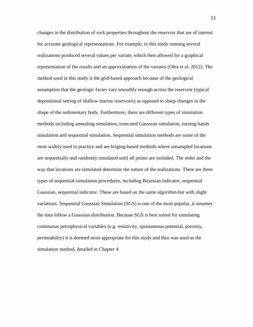
Figure 20 and 21 illustrate the spatial distribution of the wellbores, surrounded by a

bounding box representing the overall volume of the field, including color-coded R and

SP values and legend.

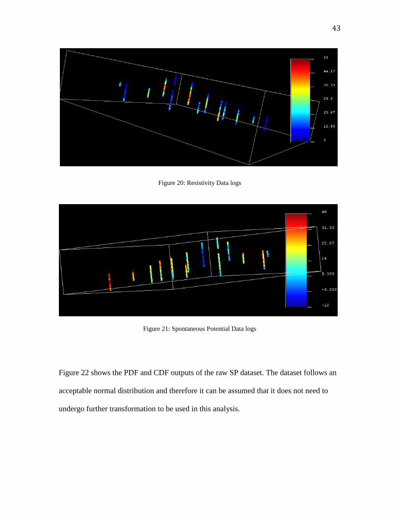
43

Figure 22 shows the PDF and CDF outputs of the raw SP dataset. The dataset follows an

acceptable normal distribution and therefore it can be assumed that it does not need to

undergo further transformation to be used in this analysis.

Figure 20: Resistivity Data logs

Figure 21: Spontaneous Potential Data logs

44

Figure 23 shows the PDF and CDF of the raw R dataset. Since the data exhibit a

significant positive skew to the right and thus is not normally distributed, it is therefore

preferable to transform this dataset to normality.

Figure 22: Spontaneous Potential CDF and PDF

Figure 23: Raw Resistivity PDF and CDF

45

The R dataset was transformed to resemble a normal distribution by using the

histogram transformation tool in the SGeMS utilities box. Figure 24 shows the PDF and

CDF of the normally transformed R dataset.

Figure 25 is a Q-Q plot of both SP and R probabilities plotting their quantiles

against each other. This graph compares the shapes of the two probability distributions

and also allows one to better determine if the data is close to a normal distribution. For

the compared probability distributions to be normal, the plotted points should lie within a

straight line. The closer all points are to a straight line the closer the samples are to a

normal distribution. This graph illustrates that there is a significant offset, indicating a

clear deviation from normality.

Figure 24: Transformed Resistivity PDF and CDF

46

Figure 26 is the Q-Q plot of the SP dataset with the normally transformed R

dataset. In this Figure the linear relationship between the two variables (points plotted

across a straighter line) indicates a more normal distribution.

Figure 25: Raw Q-Q plot between R and SP

Figure 26: Transformed Q-Q plot of SP and R

47

Figure 27 is a scatterplot of SP and R including the linear regression line

illustrating the correlation between both variables and their coefficient.

The correlation coefficient for SP and R is -0.665. The strong negative correlation

(as SP goes up R goes down and vice versa) follows the field expectation as described in

the data section. Although this correlation is not needed for ordinary kriging it provides

more useful information and allows a better evaluation for potential cokriging as a future

study.

4.2 Variogram

Several attempts experimenting with different parameters, conditions and components

were tried in the variogram modeling for this study. Correct variogram modeling requires

Figure 27: Scatterplot between R and SP

48

practice and a fair amount of guesswork. The defined variogram model is at best an

approximation of a best-fit function describing the spatial relationship of the variables in

the field.

4.2.1 Variogram Parameters

A useful initial technique to help estimate the variogram is to restrict the

maximum distance at which the variogram is computed to ensure sufficient pairs for a

given distance while still allowing for a reliable estimate of the variogram for that given

distance. A very common approach to select that restricted distance is to use around half

of the maximum possible distance within the region of assumed stationarity and use it as

the lag distance (Kelkar and Perez 2002). Because a variogram is symmetric this

approach also ensures that all pairs on either side of a given location are included in the

model, and adding 180° to a given direction provides the same variogram estimate. In

addition, another common rule of thumb is to use approximately half the distance of the

lag separation as the lag tolerance (Babish, G. 2000). It is important to note that these lag

assumptions are not necessarily relevant for every case. The conditions (geologic

structure, well geometry, depositional setting) of different oil field reservoirs can require

significantly different lag parameters. However, as noted in the geology section and

illustrated in Figure 19, the wells in this field are oriented or located in nearly a straight

line and their spacing is consistently distributed at closely uniform intervals. In addition,

the area of the field is not too large geographically so the entire reservoir system is

analyzed as a whole. These factors simplify the decision-making process for defining the

distance and direction of the variogram model.

49

Once the data is inputted into the modeling software and determined to be

appropriate for the kriging analysis, an experimental variogram model can be defined.

Figures 23 and 24 show the initial data input of the wells. The first step is to choose the

parameters that will estimate the variogram, the lag components that define the distance

and the directional components that define the direction/orientation. In SGeMS the three

lag distance components are: 1) number of lags, 2) lag separation and 3) lag tolerance and

the four lag direction components are: 1) azimuth, 2) dip, 3) tolerance and 4) bandwidth.

Figure 28 displays the lag distance and direction parameters used.

Lag distance is the product of the number of lags and the lag separation, i.e.

( ). The maximum distance between any

Figure 28: Variogram direction and distance parameters

50

two pairs of points in this field, for instance the distance between the two wells that are

farthest apart, is 4,300’. Therefore the maximum lag distance the model was initially

targeted to have is around 2,150’. After several attempts with the given directions, a lag

number of 39 and a lag separation of 55 provided promising preliminary variogram plots.

A lag tolerance half the value of the lag separation was targeted, so the value selected is

27 ( ) rounded down to the nearest whole.

The variogram for a 3D model is commonly expected to include as a minimum,

three directions: 1) a vertical directional component to account for variability with respect

to depth in any given borehole, 2) an omni-directional component to account for global

variability throughout the field, to see the overall picture, and 3) at least one horizontal

directional component covering the major directions in the field.

Four components in the SGeMS software define the directionality of the

variogram, including: 1) the azimuth, which corresponds to the direction on a planar

surface measured in degrees from 0°-360°, 2) the dip, which corresponds to the angle of

descent relative to the azimuth measured in degrees from 0°-90°, 3) the tolerance which

corresponds to the angle of tolerance of the directional variogram measured in degrees

from 0°-90°, and 4) the bandwidth, which corresponds to the maximum width of the area

resulting from the directional variogram (Remy, Boucher and Wu 2009). The azimuth

and dip, analogous to geologic strike and dip, are two important components reflecting

the major axes in a 3D environment, and the tolerance and bandwidth help further refine

the directions of interest to accommodate the intended directionality of the field. By

manipulating the variogram azimuth, dip, tolerance and bandwidth it is possible to

capture the structural geology of the field (strike, dip, rake, plunge) and hence end up

51

with a true volumetric (3D) estimation resembling the geology. Once a general direction,

(azimuth and dip) is established then the tolerance and bandwidth choices, which are

more flexible because they are based on subjective decisions, should be adjusted until an

interpretable variogram structure is identified.

4.2.2 Experimental Variogram

Three variogram directions were established: a vertical direction, an omni-

directional and a horizontal direction following the geological geometry (strike) of the oil

field reservoir. The components for all directions are shown in Figure 28. The tolerance

and bandwidth were manipulated until a clear variogram structure was obtained. Figures

29 and 30 illustrate the experimental variogram in all three directions for both datasets

after a decipherable structural trend was identified.

Figure 29: SP experimental variogram in all three directions

52

In Figures 29 and 30 if Cartesian coordinate plane orientation is assumed and the figure is

divided into four separate figures, or quadrants, Quadrant I in the upper right represents

the omni-direction, Quadrant II in the upper left represents the vertical direction,

Quadrant III in the lower left represents the horizontal direction, and Quadrant IV in the

lower right represents a plot of all the directions combined. Quadrant IV is useful to

visualize the complete extent of the entire variogram.

The first direction established is the vertical direction with an azimuth of zero, a dip of

90°, a tolerance of 5° and bandwidth of 200 (Figure 28). The interpreted variogram

Figure 30: R experimental variogram in all three directions

53

structure for each dataset in this direction as well as the fitted function is shown in

Figures 31 and 32.

The second direction established is the omni-direction with an azimuth of 0°, a dip of 0°,

a tolerance of 91° and a bandwidth of 200 (see Figure 28). The interpreted variogram

structure for each dataset in this direction as well as the fitted function is shown in

Figures 33 and 34.

Figure 31: SP Fitted vertical variogram model

Figure 33: Fitted SP Omni-directional variogram

model

Figure 32: R Fitted vertical variogram model

Figure 34: Fitted R Omni-directional

variogram model

54

The third direction established is the horizontal direction aligned along the major trend of

the wells with an azimuth of 120°, a dip of 10°, a tolerance of 40° and a bandwidth of 500

(see Figure 28). The interpreted variogram structure for each dataset in this direction as

well as the fitted function is shown in Figures 35 and 36.

4.2.3 Variogram Models

Once the distances and directions are established (see Figure 28) to get

interpretable structures (Figures 29 and 30), then the variogram can be modeled to

represent the statistical function. Two requirements that must be honored in modeling the

variogram are: 1) the condition of positive definiteness, and 2) the use of a minimum

number of parameters and models to model the variogram (Kelkar and Perez 2002).

Because the model types available in the computing software (exponential, spherical,

Gaussian) are already known to satisfy the condition of positive definiteness, by using

any of these, or linear combinations of them, it is automatically assumed that the model is

positive definite, thus satisfying condition one. As previously discussed, the variogram

estimation parameters direction and distance capture the most important reservoir

Figure 35: SP fitted horizontal variogram model Figure 36: R fitted horizontal variogram model

55

structures including geologic strike and dip, and orientation or trend of wells. It is

assumed that the essential spatial features of the oil field reservoir are thus included in the

model, which satisfies condition two. The model types available in the software are

assumed to have a sill contribution, which is a constant value after a certain lag distance

called the range, as shown in Figure 37. The components in the modeling software user

interface used to characterize the variogram model are described in the following table.

SGeMS Variogram Model Components

Interface

Input

Description

Nugget

Effect

The initial abrupt jump to the first value at the beginning of the entire

variogram model. Non-continuity only at the origin is due to either

measurement error or variation at a scale smaller than the sampling

distance.

Number of

Structures

Number of (nested) variogram structures composing the variogram

model. An accurate fit to a variogram model may be best constructed

using a combination of multiple model functions (a.k.a. nested

structures), especially to model variability at different scales.

Sill

Contribution

Effect of the sill, or the maximum variance of the variogram. Sill is the

limit (represented graphically as where the function flattens out) of the

variogram model after a specific distance a.k.a the range.

Type The type of variogram model. SGeMS includes only models for

variograms that have a sill: Spherical, Exponential and Gaussian. The

model type depends on the function used to approximate the variogram

(determines the overall shape of the model).

Ranges

(Max,Med,

Min)

Ranges along each of the three directions of the anisotropy ellipsoid in

the variogram structure (maximum, medium and minimum) used to

approximate the model. Depending on the direction(s) specified these

ranges help refine the shape/extent of the function.

Angles Measurement in degrees for each of the three angles (directions) of the

3D anisotropy ellipsoid in the variogram structure: azimuth, dip and

rake. Rotation of the angles along the orthogonal planes of a Cartesian

coordinate system positions the 3D ellipsoid in space

Table 1: Interface input description of variogram model components

56

Once a nugget constant and the number of structures in the whole variogram

model are selected, then each individual nested structure is further defined by the

subsequent parameters listed in the table: the variance contribution (sill), the variogram

function (type), and anisotropy characterized by a 3D ellipsoid defined by the ranges and

angles (Remy, N., Boucher, A. and Wu, J. 2009). This 3D ellipsoid is defined by the six

parameters of the ranges and angles where the three angles, azimuth, dip, and rake,

represent the direction of the major, medium and minor axes, and the ranges represent the

radii of the axes along the three directions. More detailed information on variogram

modeling inputs and conditions is available in the following references: Chiles and

Delfiner 1999, and Remy, Boucher. and Wu 2009. Figure 37 illustrates the main

components of a typical variogram model, including lag distance, variance, sill, nugget

and range.

Several experiments with the variogram design in terms of the modeling

components and variogram parameters were undertaken for both the SP and R datasets.

After different options were tested, the following variogram model inputs displayed in

Figure 37: Illustration of main variogram model components (based on Landscape

Toolbox Wiki 2014)

57

Figures 38 and 39 for SP and R illustrate the final variogram models used for both the

interpolation functions. These variogram models were used for the subsequent ordinary

kriging and conditional simulation procedures.

Figure 38: Complete variogram model for Spontaneous Potential

58

4.3 Interpolation

4.3.1 Kriging Parameters

Once the variogram models are defined and saved they can be loaded into

the kriging toolbox in the SGeMS program followed by simple selections of the grid, data

and the type of estimation (e.g. ordinary kriging) necessary to run the analyses. Because

the kriging algorithm used in the modeling software requires a 3D ellipsoid to be

specified in order to represent a search volume in 3D, the only remaining task was to

define the search ellipsoid (Remy, Boucher and Wu 2009). The search ellipsoid was

represented by a search space surrounding the interpolation point, and only the points that

fell within this search space were considered to take part in the kriging calculations, for

Figure 39: Complete variogram model for resistivity

59

instance in defining the extent and volume to look for values to be used in the

interpolation. The search ellipsoid, which is characterized in the same way as the

variogram anisotropy ellipsoid, consists of minimum and maximum conditioning data

(min/max number of data points to be included in the algorithm), max/med/min ranges

and the 3-directional angles. After several experimental kriging runs were conducted, the

parameters used to define the search ellipsoid for the analyses determined to be the best

were selected, provided in Table 2. . These results are described in detail in Chapter 5.

Search Ellipsoid Parameters

Conditioning Data Min Max

2 20

Ranges Max Med Min

3000 1650 200

Angles Azimuth Dip Rake

128 2 3

4.4 Validation

As part of the kriging interpolation procedure the kriging variance was also

calculated and the resulting models mapped the variance in the oil field reservoir. This

procedure can help define the areas with higher or weaker variance in the estimation.

4.4.1 Cross-validation

To know how well the models predict the values at unknown locations in the

field, in other words to test the integrity of the methods and determine their effectiveness,

it was necessary to perform validation procedures on the predicted models. An

appropriate technique is cross-validation which consists of leaving one data location out

Table 2: Search ellipsoid parameters used for kriging

60

(i.e. one well) and performing the estimation to predict the values at that excluded

location, repeating the process by removing one different well location at a time and re-

running the estimation until all the well values have been interpolated. Once the predicted

values were obtained for the data at all the measured locations, they were compared to the

known values to help determine the quality or accuracy of the model. The observed

values, which consisted of actual values from the logs, were plotted against the estimated

values predicted values from the model, then compared and contrasted to evaluate their

differences. In this manner, cross-validation at each well for both datasets was performed.

4.4.2 Statistical Comparisons

By generating several realizations using the sequential Gaussian simulation

algorithm based on the same kriging parameters, uncertainty can be characterized by the

multiple possibilities that exhibit local variation. The uncertainty at individual locations

throughout the field can be ascertained by examining the differences among several

equiprobable plots which will display the local variations and distributions in the oil field

reservoir. In this sense, if uncertainty at a particular location is relatively small then a

number of images will display similar simulated values at that location, and conversely if

uncertainty at a particular location is relatively large then a majority of images will

display the differences in simulated values at that location (Kelkar and Perez 2002).

As previously stated, the primary objective of performing a stochastic simulation

is to create a model for the probability distribution of the unknown variables. Because the

variables are conditioned to the information provided from the field data which is

61

assumed to be a true representation of the subsurface geology, then their values are

reasonably expected to fall within the limits of the simulated probability distribution.

Summary statistics on the simulation output provide a measure of the uncertainty of the

model, and specific statistical calculations on the suite of realizations provide estimated

probabilities.

Calculating the median or mean of the provided multivariate distribution where

the median (mean) at each cell is computed from the values of all realizations at that cell

location will yield a map with the highest probability of representing the true model. This

probability model can be compared to the predicted (kriged) model to provide a better

assessment of the analysis. The similarity between the predicted and the probability

models provides a degree of confidence in the estimated model. In addition to the median

probability (i.e. P50) the P10 and P90 quantiles provide uncertainty ranges or error bars

in the simulated median value, providing more confidence that the true expected mean

falls within the simulated range. A total of 48 realizations for R were obtained and a total

of 53 realizations for SP were obtained. These results are described in detail in Chapter 6.

62

CHAPTER FIVE: RESULTS

5.1 Conditional Simulation

5.1.1 Sequential Gaussian Simulation Models

In terms of final results of this thesis research, Figure 40 a-f comprises six random

realizations of SP distribution across the oil field reservoir, visualized using SGS.

Figure 40a – SP Realization 1 Figure 40b – SP Realization 2

Figure 40c – SP Realization 3 Figure 40d – SP Realization 4

Figure 40e – SP Realization 5 Figure 40f – SP Realization 6

Figure 40 (a-f): Six random SP SGS realizations

63

Figure 41 (a-f) includes 6 realizations of R distribution across the oil field reservoir.

` Figure 41a – R Realization 1 Figure 41b – R Realization 2

Figure 41c – R Realization 3 Figure 41d – R Realization 4

Figure 41e – R Realization 5 Figure 41f – R Realization 6

The calculated median (P50) as well as the P10 and P90 probability simulation models

from all the realizations are also included. Figures 42-44 illustrate the P50 map as well as

the P10 and P90 maps for R with designated color bars. Figures 45-47 illustrate the P50

map as well as the P10 and P90 maps for SP with designated color bars.

Figure 41 (a-f): Six random R SGS realizations

64

Figure 42: Resistivity P50 map

Figure 43: P10 Resistivity map

Figure 44: P90 Resistivity map

65

Figure 45: Spontaneous Potential P50 map

Figure 46: P10 Spontaneous Potential map

Figure 47: P90 Spontaneous Potential map

66

5.2 Ordinary Kriging

5.2.1 Predicted Models

The kriged model and its associated variance map for R are included as Figures 48 and

49. Figures 50 and 51 illustrate the predicted map and its associated variance map for SP.

Figure 48: Resistivity ordinary kriging interpolated map

Figure 49: Resistivity variance map from ordinary kriging model

67

5.3 Volume Explorer

The “volume explorer” tool in the SGeMS modeling software allows exploring of

the 3D distribution of properties across the estimated volume of the field. Figures 52 and

53 display a snapshot of the “inside” of the SP and R models. This is an important tool

because static images mostly show the outside of a model and may not provide an

Figure 50: Spontaneous Potential ordinary kriging interpolated map

Figure 51: Spontaneous Potential variance map from ordinary kriging model

68

adequate representation of the entire 3D volume distribution. The scale of Figure 52 is

identical to that of Figure 50 and the scale of Figure 53 is identical to that of Figure 48.

Figure 52: Spontaneous Potential 3D volume map

Figure 53: Resistivity 3D volume map

69

CHAPTER SIX: DISCUSSION AND CONCLUSION

6.1 Variogram and Simulation Model Remarks

The experimental variogram in the vertical direction (top left corner, or Quadrant

I, of Figures 29 and 30) for both datasets exhibit periodic behavior, which represents

cyclical geological processes. This is known as the “hole effect” in geostatistics and is

typically experienced when modeling a variogram in the vertical direction. In

depositional environments sediment is deposited in layers during geological events, thus

this repetition of cycles will be reflected in the vertical continuity of the layers in the

field. In these variograms the transition from one facies to another can be clearly defined.

Interpretation from both of the vertical-directional variograms indicates that the

formation is continuous in the vertical direction up to around 350’ and then becomes

discontinuous but regains continuity at greater distances. This trend is expected to

continue throughout different depths across the field. The fitted vertical variogram

functions (Figures 31 and 32) only include those values to 350’ and ignore the rest

because it is of most interest to only capture the extent of that continuity. In addition, the

average thickness of the formation is only 378’, so by modeling to 350’ we are capturing

all the continuity necessary for building a valid 3D model for this formation. The other

two variogram directions show the overall and the horizontal continuity trends in the

field, both of which exhibit very similar patterns. The fitted functions (Figures 33 through

36) were plotted in order to include most of the points. A few points which were

considered as possible local outliers were neglected in order to obtain a reasonable

structural function for the variogram model, discussed further in the project evaluation.

Overall, the trend of the study area is well captured in both of the variogram models.

70

Since all of the realizations of the conditional simulations honor the same constraints

because they are coming from the same data distribution, it is not possible that one

realization image is more likely to occur than any other. Therefore the apparent

differences between realized images is representative of the local uncertainty, and

visualizing the variability between simulations provides a reasonable assessment of

uncertainty. Provided the distribution is representative of the real oil field reservoir then

the true reservoir values are expected to fall within the bounds of the distribution while

the calculated statistical summaries of the simulations (P10, P50, P90) illustrate the

probabilities of occurrence.

6.1.1 Well ID Locations

Figure 54 is a 2D map displaying the well locations of each borehole in the

reservoir area, labeled by unique well identification number. The well ID numbers were

assigned based on the order that the wells were drilled. The spatial configuration of wells

is important to note for the discussion and interpretation of results.

71

6.2 Validation

Figures 55 and 56 (a-m) display the cross-validation results of all wells for both

datasets. The well number is the well ID number (Figure 54). The results include the

observed data (log values) plotted along with the estimated data (kriged values) versus

subsea depth. All the plots include low, medium and high value thresholds as well as

horizontal error bars of the standard deviation of the observed data for each borehole.

Figure 54: Well ID location map

72

6.2.1 Cross-validation plots

Figure 55 (a-m) provides R cross-validation graphs which represent the differences

between the observed values and the estimated values.

` Figure 55a – R Cross-Validation Well #1 Figure 55b – R Cross-Validation Well #2

Figure 55c – R Cross-Validation Well #3 Figure 55d – R Cross-Validation Well #4

Figure 55e – R Cross-Validation Well #5 Figure 55f – R Cross-Validation Well #6

Figure 55 (a-f, continued on page 73): Resistivity cross-validation results for all wells

73

Figure 55g – R Cross-Validation Well #7 Figure 55h – R Cross-Validation Well #8

Figure 55i – R Cross-Validation Well #9 Figure 55j – R Cross-Validation Well #10

Figure 55k – R Cross-Validation Well #11 Figure 55l – R Cross-Validation Well #13

Figure 55 (g-l, continued from page 72): Resistivity cross-validation results for all wells

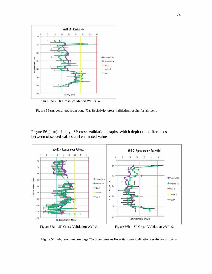
74

Figure 55m – R Cross-Validation Well #14

Figure 56 (a-m) displays SP cross-validation graphs, which depict the differences

between observed values and estimated values.

Figure 56a – SP Cross-Validation Well #1 Figure 56b – SP Cross-Validation Well #2

Figure 55 (m, continued from page 73): Resistivity cross-validation results for all wells

Figure 56 (a-b, continued on page 75): Spontaneous Potential cross-validation results for all wells

75

Figure 56c – SP Cross-Validation Well #3 Figure 56d – SP Cross-Validation Well #4

Figure 56e – SP Cross-Validation Well #5 Figure 56f – SP Cross-Validation Well #6

Figure 56g – SP Cross-Validation Well #7 Figure 56h – SP Cross-Validation Well #8

Figure 56 (c-h, continued from page 74): Spontaneous Potential cross-validation results for all wells

76

Figure 56i – SP Cross-Validation Well #9 Figure 56j – SP Cross-Validation Well #10

Figure 56k – SP Cross-Validation Well #11 Figure 56l – SP Cross-Validation Well #13

Figure 56m – SP Cross-Validation Well #14

Figure 56 (i-m, continued from page 75): Spontaneous Potential cross-validation results for all wells

77

6.3 Project Evaluation

Both of the kriged models illustrate static representations, in 3D, of the

distribution of SP and R throughout the field. The intent of kriging interpolation is to

estimate, or provide the best possible approximation of the overall continuity in this study

area. The conditional simulations provide complementary information to help determine

the local variation and quantify uncertainty in a probabilistic sense while providing a

degree of confidence in the models. The cross-validation provides a direct measurement

of the estimation accuracy.

6.3.1 Comparison of Results

Both the spontaneous potential (SP) and resistivity (R) kriged models appear to

follow an expected continuity trend based on the local geology of the field, and both of

their corresponding variance maps help indicate the local variance in their predictions.

Both of the simulations and their calculated statistical outputs provide useful

representations of the field variabilities and their probabilistic ranges. Comparing the R

kriged model with the calculated R P50 simulation mean value model (Figure 48 and

Figure 42), it appears that the overall trend remains generally consistent between both

models with the exception of a few small areas in the upper half of the field. Comparing

the SP kriged model with the calculated SP P50 simulation mean value model (Figure 50

and Figure 45) it appears that most of the continuity is also well preserved, especially in

the lower half of the field. However, small to moderate dissimilarity appears within the

upper half of the oil field reservoir. The dissimilarities that are most apparent occur

mainly near opposite edges, which is probably due to lack of data from boreholes drilled

78

near the edges of the study are (i.e. no conditioning data points). In addition, the distances

from the observed locations (i.e. logged wells) are larger, therefore we can expect greater

uncertainty in those locations. Aside from the expected larger variances near the corners

of the study area due to the edge wells being farther away from real/observed values, and

some of the localized variances that can be seen from the variance maps (Figures 49 and

51), the P10 and P90 maps appear to show a modest margin of probability in the

distribution in which the P50 median (or average) falls between the lower and upper

quantiles (P10 and P90). The noticeable differences apparent in both datasets in the upper

half of the oil field reservoir are probably related to the larger variability experienced in

the upper half of the field.

From the cross-validation it is possible to gauge the accuracy of the estimation given the

assumptions made in the modeling process, since the standard deviation error bars help

provide a “tolerance range”. Although the SP and R values obtained for the same well

locations and at the same depths do show a strong (negative) correlation, the spatial

relationships within each set differ significantly. The interpolation and validation

procedures conducted in this study help quantify these relationships. Observance of the

raw data indicates correlation trends will likely differ between both datasets due to

different modest deviations within each set of wellbores. Also, the cross-validation

results point out the individual wells that deviate the most.

The R well#1 is the well with the largest error in the R dataset, followed by the

southernmost R well#4. Although these wells plot in a consistent manner close to the

observed values, most of the calculated values fall outside the bounds of the standard

79

deviation (Figures 55 and 56). The estimated values for the rest of the wells in this

dataset appear to plot reasonably close to the observed values. However, close

examination of the results reveals that the estimations for all of the wells between R

well#1 and R well #4 (i.e. wells #11, 3, 13, 9, 8 and 14 in the lower half of the field)

appear to plot slightly better in terms of accuracy than all of the wells north of well #1

(i.e. wells #10, 2, 5 and 5 in the upper half of the field).

In contrast to the R data plots, the SP well#7 estimated values deviate the most from the

observed data, also plotting outside the bounds of the standard deviation. Most of the

other wells within this dataset plot reasonably close to the observed values, however there

are some significant differences noted, including well #4 (located at the southern edge)

and well #6 (located at the northern edge) which both show significant deviation. The

same overall field observation noted from the R results appears to also be evident in the

SP results, where all the wells in the lower half (south of the dataset outlier) provide

slightly closer approximations relative to all the wells in the upper half (north of the

dataset outlier). The “dataset outlier” for the SP values is well #7, and for the R values it

is well #1. Also included in this observation is the significant deviation of these two wells

at the boundaries, where one is located at the northern edge and one at the southern edge

of the field.

6.3.2 Interpretation

In summary, the cross-validation results as well as the compared interpolation

results indicate that the wells with slightly larger errors include the two wells at the

80

north/south edges of the field (well #4 and well #6) as well as the outlier for each dataset

(well #7 for SP and well #1 for R). Also, all of the wells north of the outlier for each

dataset (in upper half of field) show slightly higher errors than all of the wells south of

the outlier (in lower half of field).

The apparent estimation discrepancies are probably related to the fact that well #4 is the

southernmost well located in an almost isolated southeastern corner of the reservoir, and

well #6 is the northernmost well and is also the thinnest borehole (100’ of formation with

only 10 log values). The relatively larger accuracy error of these two wells located at the

study area boundaries can be attributed to their locations compared to the configuration

of other wells in the field and their less than optimal proximity to the other boreholes.

The clustered borehole locations have more conditioning data and so are expected to

provide slightly more accurate estimates. Given a general consistency between the kriged

and simulated models in addition to the same general trend expressed from the cross-

validation of both electrical datasets, the assumption can be made that the spatial

continuity in the lower half of the field is very strong (from well #4 up to somewhere

between well #7 and well#1), and in the upper half (from well #1 to well#6) it is strong

but slightly less continuous. Nevertheless, this assumption does not include the notion

that the reservoir is divided into separate segments or compartments. Based on the

observations discussed herein the integrity of the overall trend throughout the entire field

is continuous enough to consider and treat the reservoir as a whole. Based on the results

of this study, and although there a few slightly statistically deviated wells (or minor

81

localized zones), it is suggested that the reservoir is intact with a generally strong

continuity trend mimicking the geologic attitude of the field.

It is very important to provide final clarifications on the uncertainties associated with the

necessary assumptions that are expressed in the results and how it relates to the

confidence that can be attributed to the models. As mentioned in Chapters 1 and 3 the

assumption of stationarity for the entire reservoir must be made as a necessary subjective

decision. Stationarity is assumed in order to build a single geological model for the entire

study area. Also, as mentioned in Chapters 2 and 4 the wellbores are aligned along the

plane parallel to the geological strike of the field. Because all of the wells are

preferentially directed along this plane there is inherently more certainty in the data

obtained in this direction (northwest-southeast) compared to the perpendicular direction

(southwest-northeast). Due to a lack of data in the southwest-northeast direction relative

to northwest-southeast, it is apparent that there is significant directional uncertainty (i.e.

more uncertainty) in the model results along the lateral southwest-northeast direction.

Because the assumed continuities throughout the reservoir volume are constrained to and

are a direct result of the chosen variogram model parameters, the variability in the

parameters for the variogram models define the global continuity in the field. As can be

seen from the similarities between the variogram in the northwest-southeast trend and

omni-directions the continuity in the study area is preferential in the plane parallel to the

well alignment, and the uncertainty in the estimation in this direction is less significant.

Similarly, because a coherent continuity trend is captured in the vertical direction for

most of the thickness of the formation layer, the uncertainty in the estimation in this

82

direction is also less significant. According to the data in this analysis the confidence

levels (i.e. from maximum continuity to minimum continuity) follow this order, from

greatest to least: first the vertical direction, second the well alignment direction, and third

the direction perpendicular to the orientation of the wells.

Despite the many benefits of conventional estimation techniques (as discussed in Chapter

1) one of the common weaknesses of kriging, which relies on a variogram model, is that

it is completely dependent upon the input data, and because of data limitations it is

necessary to make large assumptions for an entire field which typically yield results with

directional uncertainty in continuities across the study area. As future work, to reduce the

uncertainty in this study area along the lateral plane perpendicular to the well orientation

(i.e. southwest-northeast direction), additional variogram models should be computed

using available data from wellbores drilled outside of the southwestern and northeastern

boundaries of the reservoir in order to determine any correlations with the continuities

defined in this project.

To summarize, based on all of the assumptions discussed with regards to this specific oil

reservoir, including the model parameters and directional uncertainties of the field, there

are various levels of confidence. Because of the previously mentioned similarities

between the simulated and predicted maps as well as the cross-validation results we can

assume more confidence in the variogram and continuity results for both the trends in the

vertical direction and in the direction of the wellbore alignment in the field. We can

assume less confidence in the variogram and continuity results for the trend in the

83

direction perpendicular to the wellbore alignment because of larger uncertainties in this

direction and thus weaker predictions. In addition, because of the local active geology

consisting of continuous thrust faulting that extends the reservoir along its northwest-

southeast plane and thins the geologic units of interest along its southwest-northeast

plane, it can be expected that the trend along the plane perpendicular to the geologic

strike of the study area will not be as continuous. Thus the geological representations of

the field obtained from the interpolation analyses presented as the final results of this

thesis appear to provide acceptable reservoir models that can be used at individual

discretion for subsequent engineering analyses and field operations, as long as all of the

relevant uncertainties of the field are taken into consideration.

6.3.3 Final remarks

Geostatistics is applied to several disciplines including environmental science,

oceanography, geology, meteorology and epidemiology for specific operations such as

petroleum production, water production, mining, weather prediction and even disease

spreading. Ongoing research within this field is vast and it is likely to remain a very

important modeling approach in the sciences and engineering. Although the data utilized

in this study include the electrical properties of rocks and their fluids, the same (or

similar) methodology can be applied to different datasets including hard data and soft

data values obtained from other sources such as seismic, geochemical sampling, core

sampling or remote sensing. For example, in applications to geochemistry and hydrology,

geostatistical modeling using chemical and geochemical data can help quantify the flow

and transport of subsurface constituents in aqueous systems (e.g. pollutants, solutes,

84

particles) and thus provide a better assessment of water resources including groundwater

quantity and quality (e.g. remediation of contaminant plumes and aquifer productivity).

The discipline of geostatistics is a core component of reservoir characterization and is a

necessary step to obtain an adequate geological model of the reservoir that can be

integrated into a fluid-flow numerical simulator to predict hydrocarbon production, then

further formulated into an inverse model and adjusted to match field responses. The

whole reservoir characterization-simulation-engineering process is a dynamic and

continuous process that allows scientists, engineers and operators to understand, predict

and to some extent control the reservoir in order to achieve optimal field performance.

6.4 Conclusion

The use of geostatistics provides an effective way to integrate earth science and

spatial science with engineering. This research project has demonstrated the necessary

steps to develop a geological model that characterizes the distribution of subsurface

properties using a two-point geostatistics approach. Additionally this study has directly

exemplified how GIS tools can be combined with engineering techniques based on

geological concepts and use genuine field data to solve complex real-world problems

with the aid of software interoperability. The oil field represents a conventional

petroleum reservoir and preliminary evaluation of the hard data obtained from direct

subsurface field measurements presents ordinary kriging and sequential Gaussian

simulation as valid methods for the aforementioned analysis and modeling. A satisfactory

variogram was defined incorporating geological and statistical assumptions, and used for

85

the kriging and conditional simulation interpolations to map the field properties in a

volumetric extent. The procedures taken to construct the variogram as well as the major

aspects and the different components of these techniques including the variogram

parameters, kriging parameters and interpolation conditions are discussed throughout the

report. Results include 3D static models and multiple possible realizations of the spatial

distribution of electrical properties of rocks and their fluids throughout the field domain.

And because of the direct relationship of SP and R with additional reservoir properties

and their associated characteristics (such as permeability, porosity, water saturation) the

geostatistical outputs provide useful information that can be used for further field

modeling including numerical and inverse modeling. With the information provided and

especially with the addition of subsequent engineering analyses such as reservoir

simulation and history matching, it is possible to make more informed decisions for field

operations aimed at improving petroleum development and management, including

activities such as drilling and waterflooding.

Validation procedures included statistical calculations to assess local uncertainty and

variability, as well as direct measurement comparisons. By way of comparing and

evaluating the analyses the interpretable conclusion is that the modeling techniques

performed do indeed provide a proper approach for reservoir characterization. Although

the structural continuity of the reservoir appears to retain general consistency throughout

the entire field, there is an apparent continuity trend (based on keen observations) where

the upper half of the reservoir becomes slightly less continuous relative to the lower half.

This small to modest apparent change reflected from the field continuity is probably due

to geological phenomena attributed to the major thrusting experienced in the area.

86

Moreover, the confidence level in the models and interpreted results and the associated

uncertainties due to the inherent variability and limitations in modeling subsurface

geological formations always need to be taken into consideration. The interoperability of

this project between GIS, engineering and geology alike is expected to promote the

growing field of geoinformatics and thus help bridge the gap in interdisciplinary

collaboration for data intensive research in the natural and applied sciences.

87

REFERENCES

AAPG UGM SC. One day course review: Hydrocarbon prospect in western indonesia |

AAPG UGM - SC. in American Association of Petroleum Geologists (database online).

2011 (cited 03/18 2014). Available from http://ugmsc.wordpress.com/2011/03/30/one-

day-course-review-hydrocarbon-prospect-in-western-indonesia/.

Alvarado, Vladimir, and Eduardo Manrique. 2010. Enhanced oil recovery: An update

review. Energies 3 (9): 1529-75.

Awange, Joseph L., 1969, and John B. Kyalo Kiema. 2013. Environmental

geoinformatics: Monitoring and management. Berlin ;New York: Springer Berlin

Heidelberg.

Babish, Gregg. 2000. Geostatistics without tears: A practical guide to geostatistics,

variograms and kriging. Environment Canada, Ecological Research Division,

Environmental Conservation Branch.

Bell, Julia. IPAA ranks top 10 U.S. oil and natural gas records. in Independent Petroleum

Association of America (database online). Washington, D.C., 2014 (cited March/04

2014). Available from http://www.ipaa.org/2013/07/30/ipaa-ranks-top-10-u-s-oil-

natural-gas-records/.

Burrough, P. A. 2001. GIS and geostatistics: Essential partners for spatial analysis.

Environmental and Ecological Statistics 8 (4): 361-77.

California State Parks. Geography. in State of California Department of Parks and

Recreation (database online). Sacramento, CA, 2013 (cited March/05 2014).

Available from http://www.parks.ca.gov/?page_id=21971.

Caumon, Guillaume. 2010. Towards stochastic time-varying geological modeling.

Mathematical Geosciences 42 (5): 555-69.

Chiles, Jean-Paul, and Pierre Delfiner. 1999. Geostatistics: Modeling spatial uncertainty.

New York: Wiley.

CIPA. About CIPA - california independent petroleum association. in California

Independent Petroleum Association (database online). Sacramento, CA, 2014 (cited

March/05 2014). Available from

http://www.cipa.org/i4a/pages/index.cfm?pageid=91.

Coats, K. H. 1969. Use and misuse of reservoir simulation models. Journal of Petroleum

Technology 21 (11): 1391-8.

88

Delshad, Mojdeh. 2013. Using soap to revive mature oil fields. The Way Ahead, Society

of Petroleum Engineers 9 (3): 28-9.

Deutsch, C. 2006. What in the reservoir is geostatistics good for? Journal of Canadian

Petroleum Technology 45 (4).

Division of Oil, Gas and Geothermal Resources (DOGG). 1992. CALIFORNIA OIL and

GAS FIELDS volume II – southern, central coastal, and

offshore california oil and gas fields. Sacramento, CA: State of California

Department of Conservation, TR12.

Dorsey, Ridgely. 1993. Geologic review abacherli lease mahala field: Eastern puente

hills san bernardino, california. KMT Oil Company, .

Dubrule O, and Damsleth E. 2001. Achievements and challenges in petroleum

geostatistics. Petroleum Geoscience 7 (SUPP): 1-.

Durham, D. L., and R. F. Yerkes. 1964. Geology and oil resources of the eastern puente

hills area, southern california. United States Geological Survey 420 (B): 1-62.

Enhanced Oil Recovery Institute (EOIR). Enhanced oil recovery institute: Fall 2013

newsletter. in University of Wyoming (database online). Laramie, WY, 2013 (cited

March/05 2014). Available from http://www.uwyo.edu/eori/news-and-

updates/fall2013newsletter.pdf.

ESRI. Desktop help 10.0 - working with ArcGlobe and ArcScene. in esri.com [database

online]. Redlands, CA, 2012 [cited March, 2014]. Available from

http://help.arcgis.com/en/arcgisdesktop/10.0/help/index.html#//00q8000000sv00000

0.

Gorell, Sheldon B. 1995. Using geostatistics to aid in reservoir characterization. The

Leading Edge 14 (9): 967.

GSI Works. Trimble handhelds. in Geospatial Innovations, Inc. (database online). 2009

(cited March/05 2014). Available from http://www.gsiworks.com/Handhelds.pdf.

Journel, Andre G. 2000. Geostatistics and petroleum geology. Mathematical Geology 32

(1): 139-41.

Kelkar, Mohan, and Godofredo Perez. 2002. Applied geostatistics for reservoir

characterization. Richardson, TX: Society of Petroleum Engineers Inc.

KMT Oil Company, Inc., 2014. Mr. James Kellogg. Owner and operator. Conversation.

http://owr.conservation.ca.gov/WellSearch/WellSearch.aspx

89

Krivoruchko, Konstantin. 2012. Empirical bayesian kriging: Implemented in ArcGIS

geostatistical analyst. Arcuser, Esri 15 (4): 6-10.

Landmark Software. Sequential gaussian simulation. in Halliburton (database online).

Houston, TX, 2011 (cited March/05 2014). Available from

http://esd.halliburton.com/support/LSM/DSD/DSD/5000/5000_8/Help/mergedProjec

ts/dsem/sequential_gaussian_simulation.htm.

Landscape Toolbox Wiki. Semivariogram analysis: Rangeland methods guide. in The

Nature Conservancy and the USDA Agricultural Research Service (database online).

Las Cruces, NM, (cited 03/2014 2014). Available from:

http://wiki.landscapetoolbox.org/doku.php/spatial_analysis_methods:semivariogram

_analysis.

Lowrie, William,. 2007. Geoelectricity. In Fundamentals of geophysics., 252-259.

Cambridge: Cambridge University Press, http://books.google.com/books?id=h2-

NjUg4RtEC&pg=PA254#v=onepage&q&f=false .

Madden, Christopher, and Robert Yeats. 2008. Paleoseismic and structural investigations

to determine late quaternary slip rate for the chino fault,

southeastern los angeles basin, california. Santa Ana, CA: National Earthquake

Hazards Reduction Program, 04HQGR0107.

McCammon, Richard B. ed. 1975. Concepts in geostatistics. New York: Springer-Verlag.

Myers, Donald. What is geostatistics?. in University of Arizona, Department of

Mathematics (database online). 2013 (cited March/04 2014). Available from

http://www.u.arizona.edu/~donaldm/homepage/whatis.html (accessed Tucson, AZ).

National Stripper Well Association. Stripper well facts. in National Stripper Well

Association (NSWA) (database online). Oklahoma City, OK, 2014 (cited March/04

2014). Available from http://nswa.us/custom/showpage.php?id=25.

Nobre, M. M., and J. F. Sykes. 1992. Application of bayesian kriging to subsurface

characterization. Canadian Geotechnical Journal 29 (4): 589-98.

Olea, Ricardo, Ronald Charpentier, Troy Cook, David Houseknecht, and Christopher

Garrity. 2012. Geostatistical population-mixture approach to unconventional-

resource assessment with an application to the woodford gas shale, arkoma basin,

eastern oklahoma. SPE Reservoir Evaluation & Engineering 15 (5): 554-61.

Olson, Larry J. 1977. Mahala oil field and vicinity. Sacramento, CA: California Division

of Oil & Gas, no. TR18, ftp://ftp.consrv.ca.gov/pub/oil/publications/tr18.pdf.

Optima Conservation Resources, 2014. Dr. Alberto Vasquez. President. Conversation.

http://www.ioilexchange.com

90

PetroWiki. Geostatistical conditional simulation. in Society of Petroleum Engineers

(database online). Richardson, TX, 2013 (cited March/05 2014). Available from

http://petrowiki.org/Geostatistical_conditional_simulation.

———. Glossary:Conditional simulation. in Society of Petroleum Engineers (database

online). Richardson, TX, 2013 (cited March/05 2014). Available from

http://petrowiki.spe.org/Glossary%3AConditional_simulation.

———. Kriging and cokriging. in Society of Petroleum Engineers (database online).

Richardson, TX, 2013 (cited March/05 2014). Available from

http://petrowiki.org/Kriging_and_cokriging.

———. Spontaneous (SP) log. in Society of Petroleum Engineers (database online).

Richardson, TX, 2013 (cited March/05 2014). Available from

http://petrowiki.org/Spontaneous_%28SP%29_log.

PolitiFact. A vast majority of the production in the united states comes from small

independent oil and gas companies. in Tampa Bay Times (database online). St.

Petersburg, FL, 2014 (cited March/04 2014). Available from

http://www.politifact.com/truth-o-meter/statements/2011/may/03/dan-boren/rep-dan-

boren-says-most-domestic-oil-produced-smal/.

Radhakrishna, I., and T. Gangadhara Rao. 1990. Evaluation of hydrogeochemical

parameters with spontaneous potential logs. Journal of Hydrology 114 (3): 245-57.

Ranken Energy. Useful information: A partial list of products made from petroleum (144

of 6000 items). in Ranken Energy Corporation (database online). Edmon, OK, (cited

March/05 2014). Available from http://www.ranken-

energy.com/Products%20from%20Petroleum.htm.

Remy, Nicolas, Alexandre Boucher, and Jianbing Wu. 2009. Applied geostatistics with

SGeMS: A User’s guide. Paperback ed. New York, NY: Cambridge University

Press.

Schechter, David. Formation evaluation and the analysis of reservoir performance.

chapter 9: Spontaneous potential. in Department of Petroleum Engineering, Texas A

and M University (database online). College Station, TX, 2014 (cited March/05

2014). Available from

http://www.pe.tamu.edu/blasingame/data/z_zCourse_Archive/P663_10B/P663_Sche

chter_Notes/SP%20Log.PDF.

Schlumberger. Oilfield glossary: Wireline log. in Schlumberger Limited (database

online). Houston, TX, 2014 (cited March/05 2014). Available from

http://www.glossary.oilfield.slb.com/en/Terms/w/wireline_log.aspx.

91

Schoenherr, Allan A. 1992. A natural history of california. Vol. 56. Berkeley: University

of California Press.

Sinha, A. Krishna, Ian Jackson, Peter Fox, Deborah McGuinness, Dogan Seber, Herman

Zimmerman, Zaki Malik, et al. 2010. Geoinformatics: Transforming data to

knowledge for geosciences. GSA Today 20 (12): 4-10.

Sinha, A. Krishna, David Arctur, Ian Jackson, and Linda and Gundersen. 2011. Societal

challenges and geoinformatics. Boulder, CO: Geological Society of America.

Stags, H. M., and E. F. Herbeck. 1971. Reservoir simulation models an engineering

overview. Journal of Petroleum Technology 23 (12): 1428-36.

Thomas L. Wright. 1987. Structural geology and tectonic evolution of los angeles basin.

AAPG Bulletin 71 ,

http://archives.datapages.com/data/specpubs/basinar3/images/a135/a1350001/0000/c

hapter3.pdf.

Thompson, Mark. U.S. to become biggest oil producer and energy independent. in Cable

News Network (CNN Money) (database online). London, UK, 2012 (cited March/04

2014). Available from http://money.cnn.com/2012/11/12/news/economy/us-oil-

production-energy/.

Tzimas, E., A. Georgakaki, C. Garcia Cortes, and S. D. Peteves. 2005. Enhanced oil

recovery using carbon dioxide in the european energy system. Petten, Netherlands:

Institute for Energy, European Commission Directorate-General Joint Research

Centre, EUR 21895 EN.

U.S. Energy Information Administration. How much oil does the united states consume

per year?. in U.S. Department of Energy (database online). Washington, D.C., 2012

(cited March/04 2014). Available from

http://www.eia.gov/tools/faqs/faq.cfm?id=33&andt=6.

United States Geological Survey, 2014. http://nationalmap.gov/viewer.html

United States Geoscience Information Network. 2011. California active faults.

Geothermal data project., ed. United States Geological Survey, Association of

American State Geologists, Arizona Geological SurveyArcGIS Online, Open

Geospatial Consortium.

Wilson, John P. 1955- (John Peter), and A. Stewart Fotheringham. 2008. The handbook

of geographic information science. Vol. 7. Malden, MA: Blackwell Pub.

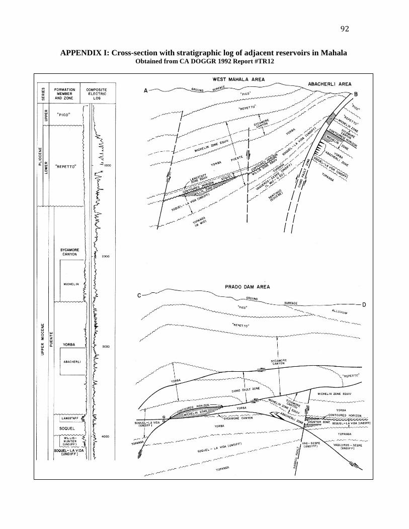
92

APPENDIX I: Cross-section with stratigraphic log of adjacent reservoirs in Mahala Obtained from CA DOGGR 1992 Report #TR12

93

APPENDIX II: Stratigraphic Column of Mahala Oilfield Obtained from DOGG Report #TR18

94

APPENDIX III: Structural Contour Map of Chino Fault Zone Obtained from USGS NEHRP 2008 report # 04HQGR0107

95

APPENDIX IV: Geological Contour Map Obtained from DOGG Report #TR18

96

APPENDIX V: Structural Contour/Isopach Map of Mahala and West Mahala

Fields Obtained from CA DOGGR 1992 Report #TR12

97

APPENDIX VI: INTEGRATED VOLUMETRIC AND NUMERICAL MODELS Obtained from combining Matlab, SGeMS, Excel and ArcGIS using Reservoir Data