geological 3d model of the investigation niche in onkalo
TRANSCRIPT

July 2014
Working Reports contain information on work in progress
or pending completion.
Noora Koittola
Posiva Oy
Working Report 2014-35
Geological 3D Model of the InvestigationNiche in ONKALO, Olkiluoto,
Southwestern Finland


ABSTRACT
The main goal of this Master of Science Thesis was to create a geological 3D-model of the investigation niche 3 and its surroundings. The model were created for the needs of the rock mechanical back analysis. This study is a part of Posiva's regional studies for characterization of the bedrock. Totally 4 models were created: lithological model, foliation model, fracture model, and physical rock property model. Besides the modeling, there was also made a study of the migmatite structures in the niche. Used geological and geophysical methods were drill core loggings, tunnel mapping, ground penetration radar, mise-á-la-masse and drill hole geophysics. Four rock types exist at the niche area: veined gneiss, pegmatite granite, diatexitic gneiss and quartz gneiss. The lithological units were modeled primary with the drill core loggings, tunnel mapping and ground penetrating radar. The major lithological units followed the main foliation direction (south dipping). So the continuations were fairly easy to model in the walls and roof, where the data was lacking. Foliation and fractures were modeled as discs, with mid-points at the measurement points of the structure. There were two main foliation directions 164/46 and 62/39. Fractures were more scattered but three fracture sets can be separated: 156/34, 270/85 and 342/83. The first set is mainly from the drill core loggings, second and third from tunnel mapping. Used methods in foliation model were drill core loggings, tunnel mapping and drill hole geophysics. In fracture model used data was from drill core loggings, tunnel mapping, mise-á-la-masse measurements and drill core geophysic. Four anomalous zones were detected with the drill hole geophysics. Three of these zones were associated with intensely fractured zones and one was connected to exceptionally high mica content in the gneiss. Rocks of Olkiluoto are divided into gneisses and magmatic rocks in the geological mapping. Actually almost all Olkiluoto's rocks are more or less migmatites. The migmatite classification is created at the moment so it was reasonable also study the migmatite structures. The recognized structures were schlieren, homophanous, veined and the border of metatexite and diatexite. Besides the modeling, there was also made a quality control of the used data and methods. During the modeling was also located a slickenside fracture set under the niche. There is a possibility that this fracture set is connected to one of the brittle fault zones (bfz-265). Despite this, these structures cannot be combined before additional studies. Keywords: Olkiluoto, ONKALO, final disposal of nuclear waste, Surpac, 3D-model, structural geology, geophysics, rock mechanic, POSE experiment, back analysis, lithology, foliation, fracture, anomaly, migmatite, quality inspection, bfz-265.

Geologinen 3D malli ONKALO:n tutkimuskuprikasta 3, Olkiluodossa
TIIVISTELMÄ
Tutkimuksessa luotiin 3D-malli tutkimuskuprikka 3:sta ja sen lähialueen geologiasta. Mallit luotiin erityisesti kalliomekaanisen takaisinlaskennan tarpeisiin. Tutkimus toimii-kin osana Posiva Oy:n aluetutkimuksia, joiden tavoitteena on karakterisoida Olkiluodon kallioperää. Malleja luotiin yhteensä 4 kappaletta: litologiamalli, foliaatiomalli, rakoi-lumalli ja malli kiven fysikaalisista ominaisuuksista. Mallinnuksen lisäksi kuprikasta tehtiin migmatiittirakenteiden tutkimus. Mallinnuksessa käytettyjä geologisia ja geofy-sikaalisia metodeja olivat kairasydänloggaukset, tunnelikartoitus, maatutkaus, lataus-potentiaalimittaukset ja kairareikägeofysiikka.
Litologiamalliin mallinnettiin solideina kuprikan alueella esiintyneet neljä kivilajia: suonigneissi, pegmatiittigraniitti, diateksiittinen gneissi ja kvartsigneissi. Yksiköt mal-linnettiin ensisijaisesti kairasydänloggausten, tunnelikartoituksen ja maatutkausten avul-la. Suurimmat kivilajiyksiköt seurasivat vallitsevaa foliaatiosuuntaa (etelään kaatuva), joten jatkeita oli helppo mallintaa myös kattoon ja seiniin, joista data oli puutteellista.
Foliaatio ja rakoilu mallinnettiin disc-tasoina, joiden keskipiste sijaitsee rakenteen mit-tauspisteessä. Foliaatiosuuntia ilmeni kaksi: 164/46 ja 62/39. Rakoilu oli epäsäännölli-sempää, mutta kolme päärakosuuntaa erottui: 156/34, 270/85 ja 342/83. Näistä ensim-mäinen on määritelty lähinnä kairasydänloggauksista ja kaksi viimeistä ovat tunnelikar-toituksesta. Foliaatiomallin luonnissa käytettiin dataa kairasydänloggauksista, tunneli-kartoituksesta ja kairareikägeofysiikasta. Rakoilumalli luotiin loggausten, kartoituksen, latauspotentiaalin ja reikägeofysiikan avulla.
Reikägeofysiikassa havaittiin neljä fysikaalisesti anomaalista vyöhykettä kuprikan alta. Näistä kolme liittyi ensisijaisesti intensiivisesti rakoilleeseen gneissiin ja yksi gneissin poikkeuksellisen korkeaan kiillepitoisuuteen.
Olkiluodon kivilajit jaotellaan kartoituksessa ja mallinnuksessa gneisseihin ja syväki-viin. Todellisuudessa Olkiluodon kivet ovat kaikki enemmän tai vähemmän migmatiit-teja. Parhaillaan ollaan luomassa alueen migmatiittirakenneluokittelua, joten tähänkin työhön otettiin mukaan myös kuprikan migmatiittien tarkastelu. Kuprikasta löytyneet rakenteet olivat suurimmaksi osaksi eriasteisia schlieren -rakenteita. Kuprikan alueelta löydettiin myös homofaaninen rakenne, suonirakenne sekä metateksiittisen ja diatek-siittisen migmatiitin raja.
Mallinnuksen lisäksi työssä haluttiin keskittyä käytetyn datan ja luotujen mallien laatutarkasteluun sekä niiden käytettävyyden arviointiin. Mallinnuksen aikana löydettiin kuprikan alta myös intensiivisesti rakoillut haarniskarakosetti, joka viittaa mahdolli-suuteen, että kuprikan alla kulkee hauraan ruhjevyöhykkeen (bfz-265) jatke. Näiden rakenteiden yhdistäminen tarvitsee kuitenkin vielä lisätutkimuksia.
Asiasanat: Olkiluoto, ONKALO, ydinjätteen loppusijoitus, Surpac, 3D-mallinnus, rakennegeologia, geofysiikka, kalliomekaniikka, POSE-koe, takaisinlaskenta, litologia, foliaatio, rakoilu, anomalia, migmatiitti, laatutarkastelu, bfz-265.


1
CONTENTS 1. INTRODUCTION ............................................................................................ 3 2. REGIONAL GEOLOGY .................................................................................. 5
2.1. Geology of southern Finland .................................................................... 5 2.1.1. Tectonic Evolution .............................................................................. 7
2.2 Geology of Satakunta Area ....................................................................... 8 2.3 Geology of Olkiluoto Island ..................................................................... 11
2.3.1 Lithological Classification used in Geological Mapping ..................... 11 2.3.2 Migmatite Classification .................................................................... 11 2.3.3 Deformation and Metamorphism ....................................................... 14
3. THIRD INVESTIGATION NICHE .................................................................. 17 3.1 Excavation History .................................................................................. 17 3.2 POSE Experiment ................................................................................... 19
4. DATA AND METHODS ................................................................................ 23 4.1 Geological Methods ................................................................................ 23
4.1.1 Drill Core Loggings ........................................................................... 23 4.1.2 Geological Mapping of the Niche and Experiment Holes .................. 24
4.2 Geophysical Methods .............................................................................. 27 4.2.1 Ground Penetrating Radar ................................................................ 27 4.2.2 Mise-á-la-Masse Surveys ................................................................. 30 4.2.3 Drill Hole Geophysics ........................................................................ 33
4.3 3D-modeling Methods ............................................................................. 35 5. RESULTS ..................................................................................................... 37
5.1 Lithological Model ................................................................................... 37 5.1.1 Modeled mica bands ......................................................................... 43
5.2 Foliation Model ........................................................................................ 44 5.3 Fracture Model ........................................................................................ 47 5.4 Physical Rock Property Model ................................................................ 48 5.5 Modeling Files ......................................................................................... 49 5.6 Migmatite Structures in the Investigation Niche ...................................... 49
6. DISCUSSION ............................................................................................... 55 6.1 Applicability and Representativeness of the Data and Methods ............. 55 6.2 Representativeness of the Model ............................................................ 56 6.3 Correlation with the Site Model ............................................................... 57
7. SUMMARY AND CONCLUSIONS ............................................................... 61 8. ACKNOWLEDGEMENTS ............................................................................. 65 9. REFERENCES ............................................................................................. 67 APPENDIX 1. APPENDIX 2. APPENDIX 3. APPENDIX 4. APPENDIX 5. APPENDIX 6. APPENDIX 7. APPENDIX 8.

2

3
1. INTRODUCTION
Posiva Oy is responsible for implementing the final disposal programme for spent nuclear fuel of its owners Teollisuuden Voima Oy and Fortum Power & Heat. Spent nuclear fuel is planned to be disposed at a depth of 400-450 meters in crystalline bedrock on the Olkiluoto site. Posiva submitted an application for a construction license for the disposal facility at the end of 2012 and the active phase of final disposal is scheduled to begin at 2022. This Master of Science Thesis is part of Posiva's site studies for the characterization of the bedrock. The aim of this Thesis is to create geological 3D model of the third investigation niche based on geological and geophysical data.
Posiva has an ongoing rock mechanical POSE (Posiva's Olkiluoto Spalling Experiment) experiment; the goals of the experiment are to settle in situ stress conditions and spalling strength of the bedrock as well as to "act as a Prediction–Outcome exercise" (Johansson et al 2013). However the results of the POSE experiment were complicated due to heterogenous lithology. For that reason, the rock mechanical back analysis cannot be completed without a detailed geological model. In the future this model will be in a key role in determining if geological features such as lithology, foliation or fracturing have an effect on the mechanical properties of the bedrock.
Versatile geological and geophysical data were used in the modeling. Systematic geological mapping was carried out in the POSE niche and in the three experiment holes. 97 drill cores were drilled and investigated from the niche. Also diverse geophysical data related to the POSE experiment and EDZ (Excavation Damage Zone) studies within the niche were available for use. These data comprise ground penetrating radar, mise-à-la-masse and drill hole geophysics. The model itself was created with Geovia Surpac 3D modeling software.
During the work, four separate models will be created: lithological model, foliation model, fracture model and physical rock property model. Lithology is modeled as solids, foliation and fracturing as a discs and physically anomalous features as zones. Apart from the modeling, the migmatite structures of investigation niche 3 will also be studied with the assistance of Aulis Kärki at the University of Oulu.

4

5
2. REGIONAL GEOLOGY
2.1. Geology of southern Finland
The bedrock of southern Finland can be divided into five separate terrains. These are Savo belt (SB), Central Finland Granitoid Complex (CFGC), Tampere belt (TB), Häme belt (HB) and Uusimaa belt (UB) (Figure 1) (Vaasjoki et al. 2005). Savo belt locates at the area, where Arcaean and Fennoskandian shields face. Tampere belt and Central Finland Granitoid Complex form most of the central Finland and Häme and Uusimaa belts form most of the southern Finland.
According to Vaasjoki et al. (2005), dominant rock types of the Savo belt are mica gneisses, which contain volcanic rocks, graphite schists, black schists, and carbonate rocks as interlayers. Magmatic rocks are 1.92 Ga gneissic tonalites and 1.89-1.88 Ga granitoids (Vaasjoki et al. 2005). Savo belt (SB) is characterized by several shear zones (Vaasjoki et al. 2005).
Central Finland Granitoid Complex (CFGC) consists mainly of 1.89-1.88 Ga synkinematic tonalites, granodiorites and granites as well as 1.88-1.86 Ga postkinematic quartz monzonites and granites (Vaasjoki et al. 2005). According to Vaasjoki et al. (2005), minor areas of the complex consist of subvolcanic intermediate rocks, mafic igneous rocks and remnants of supracrustal belts.
According to Vaasjoki et al. (2005), Tampere belt (TB) consists of 1.90-1.89 Ga intermediate and felsic volcanic rocks as well as turbiditic mica schists with conglomerate interlayers. Also mafic volcanic rocks occur. The youngest rocks are 1.88 Ga granitoids which crosscuts the supracrustal rocks (Vaasjoki et al. 2005).
Häme belt (HB) is characterized by volcanic rocks. According to Vaasjoki et al. (2005), only at the western parts of the belt some metasedimentary rocks occur. Main igneous rock types are 1.88 Ga granitoids and 1.84-1.82 Ga granites which crosscuts the supracrustal rocks (Vaasjoki et al. 2005).
Uusimaa belt (UB) is sedimentary dominated belt that contains mica schists and gneisses with carbonate rock interlayers. According to Vaasjoki et al. (2005), also felsic sedimentary rocks of volcanic origin are typical to the Uusimaa belt. The composition of volcanic rocks varies usually from mafic to intermediate but in western parts of the belt volcanism is bimodal (Vaasjoki et al. 2005). Similarly to Häme belt, igneous rocks are 1.88 Ga granitoids and 1.84-1.82 Ga granites which crosscuts the supracrustal rocks (Vaasjoki et al. 2005).
6
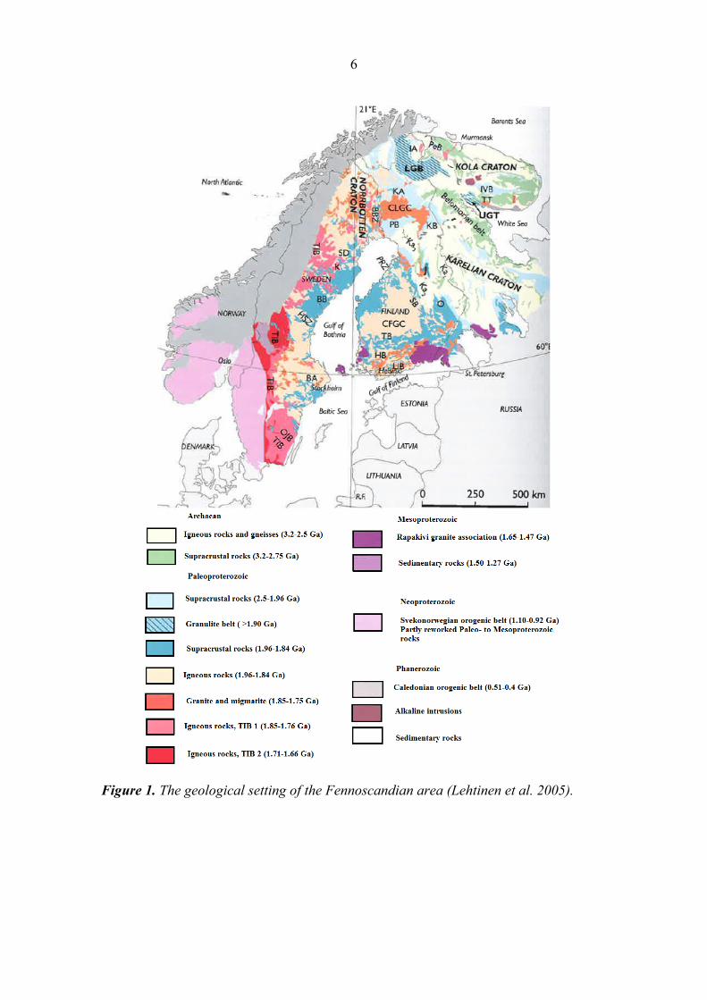
Figure 1. The geological setting of the Fennoscandian area (Lehtinen et al. 2005).

7
2.1.1. Tectonic Evolution
Fennnoscandian Shield has formed between 2.06 - 1.77 Ga during the five orogenies: Lapland-Kola orogen, Lapland-Savo orogen, Fennian orogeny, Svecobaltic orogeny and Nordic orogeny (Lahtinen et al. 2005) (Figure 2). According to Lahtinen et al. (2005), these orogenies partly overlap in time and space. Even though, before the active stage of orogenies started, Arcean craton started to break up. Multiple rifting of the craton occurred at 2.5-2.1 Ga. The location of the breakup followed the present western margin of the Karelian craton and created marginal basins along the edge.
Lapland-Kola orogen was most active at 1.94-1.91 Ga ago. The orogen started by subduction related magmatism at Inari area and Tersk terrain (Lahtinen et al. 2005). According to Lahtinen et al. (2005), at 1.93 Ga subduction was active towards the southwest under the Lapland-Kola area and back-arc basin formed. Back-arc basins were shortened because of Kola craton collided to Karelian craton at 1.93-1.91 Ga (Lahtinen et al. 2005). The accretion of Tersk terrain occurred at ca. 1.91 Ga. The orogenic collapse of the Lapland-Kola orogen occurred at 1.88-1.87 Ga and this caused thinning of the crust (Lahtinen et al. 2005).
Collision of the Lapland-Savo orogeny started 1.92 Ga ago when Kittilä allocton emplaced and at the same time the Savo belt accreted to the Keitele microcontinent (Lahtinen et al. 2005). According to Lahtinen et al. (2005), continent-continent collision of Karelia craton and Keitele microcontinent in Finland and Norrbotten microcontinent in Sweden occurred at 1.92-1-89 Ga. Bothnian microcontinent collided to Norbotten and Keitele 1.90 Ga (Lahtinen et al. 2005). This collision caused magmatism which formed Knaften arc at 1.90 Ga (Lahtinen et al. 2005).
Between Lapland-Savo and Fennian orogenies, "the accretion of Keitele microcontinent and Karelia craton resulted in a subduction reversal" which caused the extension at the southern edge of Keitele microcontinent (Lahtinen et al. 2005). According to Lahtinen et al. (2005), in Sweden, the docking of Bothnia and Norrbotten led to a subduction switch-over. This caused a new subduction zone under either oceanic crust or Bothnia microcontinent at 1.89-1.87 Ga (Lahtinen et al. 2005).
During the Fennian orogeny (1.89-1.85 Ga) the tectonic events differ in time across the Gulf of Bothnia from Finland to Sweden because the fault system separated Keitele and Bothnia microcontinents (Lahtinen et al. 2005). According to Lahtinen et al. (2005), oceanic plate subducted towards south and this caused the combination of Tavastia island arc and Bergslagen microcontinent (Lahtinen et al. 2005). After that, Tavastian island arc collided to Keitele microcontinent 1.89 Ga ago. The major collisional stage is associated with voluminous continental growth in current area of Central Finland (Lahtinen et al. 2005).
Lapland-Savo orogeny attempted to collapse simultaneously with the collisional stage of Fennian orogeny (Lahtinen et al. 2005). According to Lahtinen et al. (2005), this caused related magmatism at central Finland's area. At the end of Fennian orogeny, subduction reversal occurred at the southern margin of the shield. Also the boundaries between Karelia-Keitele and Keitele-Tavastian stabilized at the time between Fennian orogeny and Svecobaltic orogeny (Lahtinen et al. 2005).

8
Svecobaltic orogeny occurred at 1.84-1.80 Ga when Sarmatia continent collided obliquely to the southern parts of Fennoscandian continent (Lahtinen et al. 2005). According to Lahtinen et al. (2005), this collision caused migmatization, thrusting and folding in the southern Finland. The cyclic nature of events caused the complicated stacking structure to the bedrock of southern Finland (Lahtinen et al. 2005). In the southwestern parts of Fennoscandia, Andean-type magmatic stage occurred (ca. 1830 Ma) associated with the collision (Lahtinen et al. 2005).
Nordic orogeny occurred at 1.82-1.79 Ga ago and the presently exposes as Transcandinavian Igneous Belt (TIB) (Figure 1) (Lahtinen et al. 2005). According to Lahtinen et al. (2005), the orogeny is proposed as continent-continent collision, possibly between Fennoscandia and Amazonia. The main effects of the collision can be seen at the central parts of the Fennoscandian Shield, currently locating in Sweden and Norway (Lahtinen et al. 2005).
Figure 2. Tectonic evolution of Fennoscandia.
2.2 Geology of Satakunta Area
The supracrustal rocks of Satakunta formed during the evolution described in Chapter 2.1.1 (Paulamäki 2009). In Satakunta area these rock types forms a belt of pelitic migmatites (PEMB) at southwest and a belt of psammitic migmatites (PSMB) at northeast (Paulamäki 2002).
Metamorphism in Satakunta area took place in 750-800°C and 5-6 kb and ductile deformation and migmatitization are connected to close to the peak of metamorphism (Korhonen et al. 2010). In Figure 3, the rocks of Olkiluoto island are marked as mica schists and mica gneisses.
After orogenies, rapakivi magmatism of southern Finland took place at 1.65-1.55 Ga. During this stage, the Laitila rapakivi batholith and the Eurajoki stock were intruded 1.58 Ga (Vaasjoki 1996).

9
Jotnian sedimentary rocks deposited ca. 1.4-1.3 Ga ago (Korhonen et al. 2010). The Satakunta sandstone deposited to the graben structure (Korhonen et al. 1993, Korja &Salonen 1995). According to Korhonen et al. (1993), the depositional setting of the Satakunta sandstone is comparable with fluvial delta. The exact deposition period cannot be defined, but it is supposed, that deposition took place between rapakivi magmatism and diabase magmatism.
Postjotnian olivine diabase veins and sills are the youngest rocks (1270-1250 Ma) in the Satakunta area (Korhonen et al. 2010). These veins are usually north-south trending (Suominen 1991, Veräjämäki 1998) and the sills are gently dipping or horizontal.

10
F
igu
re 3
. Lit
holo
gy o
f the
Sat
akun
ta a
rea.
Olk
iluo
to I
slan
d is
mar
ked
wit
h th
e bl
ack
squa
re (
Pos
iva
Oy
2011
).

11
2.3 Geology of Olkiluoto Island
2.3.1 Lithological Classification used in Geological Mapping
In geological mapping, the rocks of Olkiluoto are firstly classified as variably migmatized high-grade metamorphic rocks and magmatic rocks (Posiva Oy 2011) and rocks are further classified according to the BGS (British Geological Survey) standards (Mattila 2006). According to Mattila (2006) the types of metamorphic gneisses are stromatic gneiss (SGN), veined gneiss (VGN), diatexitic gneiss (DGN), mica gneiss (MGN), quartz gneiss (QGN), mafic gneiss (MFGN) and tonalitic-granodioritic gneiss (TGG). The magmatic rocks are pegmatite granite (PGR), K-feldspar porphyry (KFP) and diabase (MDB) (Mattila 2006). A closer classification of the gneisses is shown in Figure 4. This classification is used in tunnel mapping and drill core logging.
Figure 4. Classification of the gneisses in Olkiluoto (Aaltonen et al. 2010).
2.3.2 Migmatite Classification
The rocks in Olkiluoto can also be divided by the state of migmatitization. Migmatites are mixtures, consisting of metamorphic looking and igneous looking rock components (Kärki 2014). In literature, there are several different definitions for the term migmatite and as examples the definitions of Sederholm (1907) and Mehnert (1968) are mentioned here. According to Sederholm (1907) migmatite is "a mixture of two genetically different constituents of which one is of a more intrusive type than the other". Examples of these rocks are gneissic granites, which show structures characteristic to the partial melting (Sederholm 1907). According to Mehnert (1968) migmatite is "megascopically composite rock consisting of two or more petrographically different parts. One is a country rock in a more or less metamorphic state and the other is pegmatitic, aplitic, granitic or generally plutonic appearance" (Mehnert 1968). In any case, whatever the

12
definition is, migmatites are "closely associated with high-grade metamorphism but equally with magmatic prosesses" (Kärki 2014).
Migmatites of Olkiluoto are formed in high temperature in prograde or/and retrograde metamorphism where partial melting or anatexis occurs in pre-existing rocks (Kärki et al. 2006). Migmatized rocks can be divided into paleosome and neosome. Paleosome is a remnant of source rock and neosome consists of melanosome and leucosome (Kärki 2014). According to Sawyer (2008), three different leucosome types can be identified: in situ leucosome, in-source leucosome and leucocratic dikes.
The intensity of migmatitization divides rocks into two main types: metatexites and diatexites (Figure 5). In metatexites, several discrete components can be detected and the rock is overall heterogenous (Kärki 2014). According to Kärki (2014), paleosome is identifiable and pre-migmatitization structures, for example layering and foliation, are identifiable. The neosome content is usually something between 20-30% but it can vary. Diatexites are more intensively melted rocks, where paleosome and pre-structures are not always detectable (Kärki 2014). According to Kärki (2014), neosome forms a major part of diatexites and the appearance of neosome varies. For that reason diatexites are difficult to classify. A more specific classification of migmatites is based on visible factors and "variables describing the properties of the neosome and paleosome" (Engström 2014).
Figure 5. The classification of migmatites of the Olkiluoto island (Kärki 2014).
Migmatites of Olkiluoto can be divided into ten different classes based on their structures. These structures are dike-structure, net-structure, breccia-structure, patch-structure, layer-structure, vein-structure, schollen structure, schlieren structure, nebulitic
13
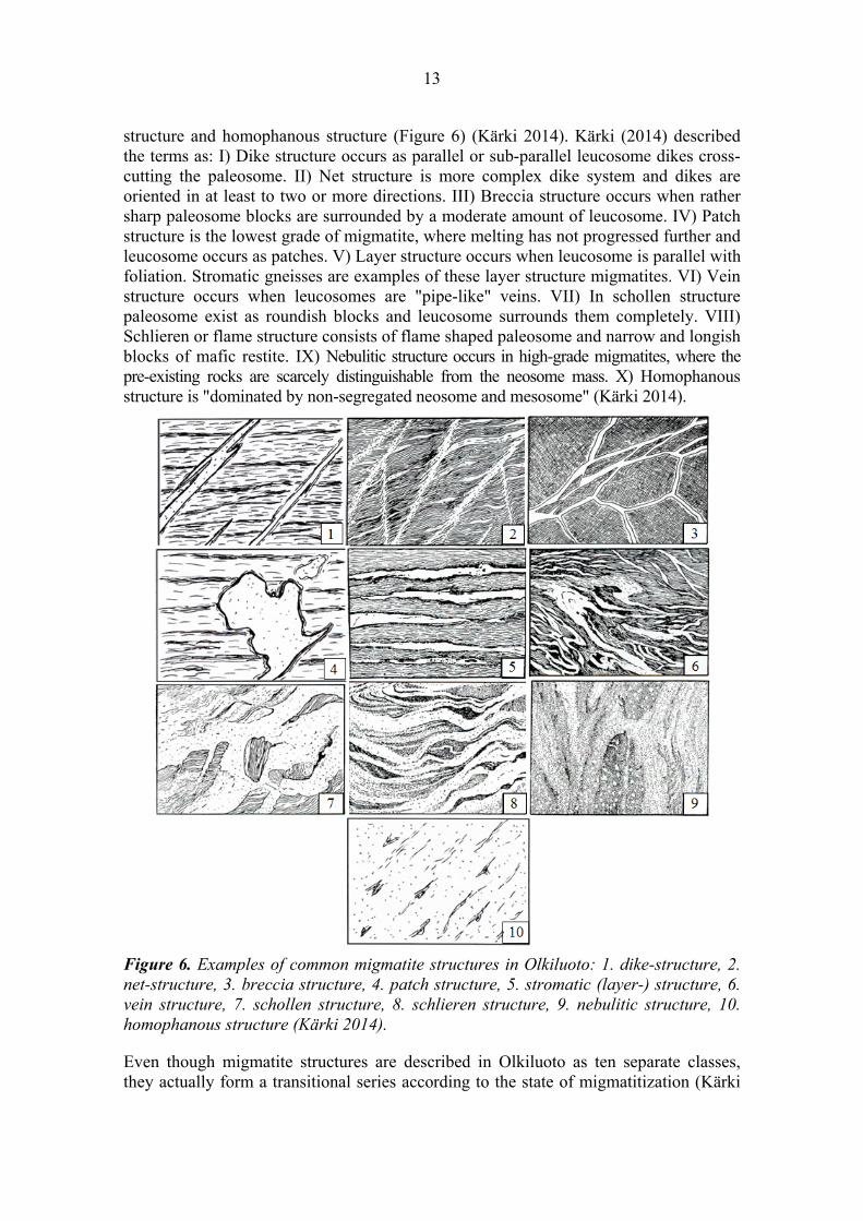
structure and homophanous structure (Figure 6) (Kärki 2014). Kärki (2014) described the terms as: I) Dike structure occurs as parallel or sub-parallel leucosome dikes cross-cutting the paleosome. II) Net structure is more complex dike system and dikes are oriented in at least to two or more directions. III) Breccia structure occurs when rather sharp paleosome blocks are surrounded by a moderate amount of leucosome. IV) Patch structure is the lowest grade of migmatite, where melting has not progressed further and leucosome occurs as patches. V) Layer structure occurs when leucosome is parallel with foliation. Stromatic gneisses are examples of these layer structure migmatites. VI) Vein structure occurs when leucosomes are "pipe-like" veins. VII) In schollen structure paleosome exist as roundish blocks and leucosome surrounds them completely. VIII) Schlieren or flame structure consists of flame shaped paleosome and narrow and longish blocks of mafic restite. IX) Nebulitic structure occurs in high-grade migmatites, where the pre-existing rocks are scarcely distinguishable from the neosome mass. X) Homophanous structure is "dominated by non-segregated neosome and mesosome" (Kärki 2014).
Figure 6. Examples of common migmatite structures in Olkiluoto: 1. dike-structure, 2. net-structure, 3. breccia structure, 4. patch structure, 5. stromatic (layer-) structure, 6. vein structure, 7. schollen structure, 8. schlieren structure, 9. nebulitic structure, 10. homophanous structure (Kärki 2014).
Even though migmatite structures are described in Olkiluoto as ten separate classes, they actually form a transitional series according to the state of migmatitization (Kärki
14
2014). For example as the degree of migmatitization increases, dike structure gradually transforms into net structure or breccia structure and ultimately to schollen structure.
2.3.3 Deformation and Metamorphism
The metasedimentary rocks of Olkiluoto island metamorphosed in upper amphibolite facies, at the temperature of 650-700°C and at the pressure of 4-5 kb (Aaltonen et al. 2010) and they deformed ductilely in four stages (D1-D4) (Engström 2014).
The oldest visible structures are primary lithological lamination S0 and slightly segregated schistosity S1 (Engström 2014). The deformation phases D2, D3 and D4 can be separated from each other. During the D2, the pervasive east-west oriented S2 foliation was formed (Engström 2014). According to Engström (2014), also the migmatization was intense during the D2.
The D3 phase deformed primary structures and secondary patterns that were formed earlier. Migmatites formed F3 folds and ductile shear zones, parallel with the S3 axial planes, were formed. Also dextral shearing occurred in S2 structures and thrust faults were formed (Engström 2014). Engström (2014) continues that also earlier S2 foliation rotated mostly parallel to F3 axial surfaces during the D3. Migmatitization continued through the D3 and neosome veins and patches were formed.
During the D4 stage, axial planes of F4 folds and foliation rotated to NNE-SSW (Engström 2014). Small scale, S4 oriented dextral shears are also associated with this deformation phase. D4-deformation was most intense at eastern part of the island (Engström 2014). According to Engström (2014), the pinitization of the cordierites and the formation of a migmatites, which contains quartz and k-feldspar porphyroblast, are associated with this deformation phase.
In addition to ductile deformation, some semi-brittle and brittle structures also exist. Faulting types in Olkiluoto are thrust faults and strike-slip faults (Aaltonen et al. 2010). According to Aaltonen et al (2010), thrust faults are typically south-east dipping and strike-slip faults are north-east to south-west striking.
There are also three main fracture directions in Olkiluoto. According to Posiva Oy (2011), most of the fractures are gently (0-40°) dipping to the S or SSE. In addition two steeply-dipping N-S and E-W striking fracture clusters are observed (Posiva Oy 2011). The lithological map of Olkiluoto is shown in Figure 7.
In post D4-stage the rocks continued to cool, but some features, connected to lowering temperature can be identified from the rocks of Olkiluoto island. Low temperature (100-300°C) hydrothermal fluids, related to the rapakivi magmatism in the Satakunta area (Haapala 1977), caused some alterations, specifically connected to the structures of brittle deformation. The most typical hydrothermal alterations in Olkiluoto are sulphidization and kaolinization. In sulphidization, the alteration product is generally pyrite (Aaltonen et al. 2010). According to Aaltonen et al. (2010), there is also illitization which can be seen in altered leucosomes and in several thrust faults.

15
Fig
ure
7. L
itho
logy
of O
lkil
uoto
Isl
and.
The
loca
tion
of O
NK
AL
O is
mar
ked
on th
e m
ap w
ith
blac
k sq
uare
(P
osiv
a O
y 20
11).

16

17
3. THIRD INVESTIGATION NICHE
3.1 Excavation History
The third investigation niche is located in ONKALO tunnel chainage level 3620 at -345 meters below the surface (Posiva Oy 2011) (Figure 8).
Figure 8. The location of the investigation niche 3 in ONKALO.
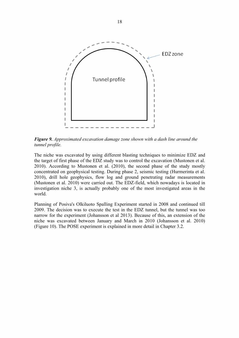
The niche was excavated from June 2009 to November 2009 and it was originally used for EDZ (Excavation damage zone) studies and sometimes referred to as the EDZ tunnel (Hurmerinta et al. 2010). Excavation with explosives causes a damage zone in the surrounding rock (Figure 9), creating possible hydraulic connections. This damage extends a maximum of 30-40 cm outside the tunnel profile in ONKALO.
The studying of these zones is therefore critical for tunnel constructing and long term safety (Mustonen et al. 2010, Tsang et al. 2005). Even though, the main goal of the EDZ studies is to develop an excavation technique that minimizes the damage (Tsang et al. 2005). The ground penetrating radar has produced reliable results in Olkiluoto and it is therefore the most used method in EDZ studies (Mustonen et al. 2010). For example in a study by Cal and Kaisers (2005), microseismics and acoustic emission was used to create a numerical model.
18
Figure 9. Approximated excavation damage zone shown with a dash line around the tunnel profile.
The niche was excavated by using different blasting techniques to minimize EDZ and the target of first phase of the EDZ study was to control the excavation (Mustonen et al. 2010). According to Mustonen et al. (2010), the second phase of the study mostly concentrated on geophysical testing. During phase 2, seismic testing (Hurmerinta et al. 2010), drill hole geophysics, flow log and ground penetrating radar measurements (Mustonen et al. 2010) were carried out. The EDZ-field, which nowadays is located in investigation niche 3, is actually probably one of the most investigated areas in the world.
Planning of Posiva's Olkiluoto Spalling Experiment started in 2008 and continued till 2009. The decision was to execute the test in the EDZ tunnel, but the tunnel was too narrow for the experiment (Johansson et al 2013). Because of this, an extension of the niche was excavated between January and March in 2010 (Johansson et al. 2010) (Figure 10). The POSE experiment is explained in more detail in Chapter 3.2.

19
Figure 10. The layout differences in investigation niche 3 between the present (left) and before the extension (right).
3.2 POSE Experiment
After the extension of the niche, preparations for POSE (Posiva's Olkiluoto Spalling Experiment) started in 2010. The experiment was divided into phase 1, 2 and 3. The target of the first and second phases was to determine the spalling strength of the veined gneiss, confirm the in situ stress conditions at -345 m and to "act as a Prediction–Outcome exercise" (Johansson et al. 2014).
The first phase was to drill two nearly full scale deposition test holes, which are called experiment holes 1 and 2 (ONK-EH1 and ONK-EH2) (Johansson et al. 2014). Johansson et al. (2014) continues that a 90 cm thick rock pillar was left between the

20
experiment holes. The first phase is therefore also referred to as the Pillar test. The layout of ONK-EH 1 and 2 is shown in Figure 11. The aim was to focus the high stresses to the pillar and cause spalling and damage into the pillar (Johansson et al. 2014).
Figure 11. The layout of investigation niche 3 and experiment holes 1 and 2.
The second phase of the POSE experiment was heating of the rock mass near the pillar. Heating increases the stress state in the pillar and spalling should occur. According to Johansson et al. (2014), two heaters were installed at the north end of the pillar and two at the south end. During heating, ONK-EH2 was filled with sand (Johansson et al. 2014). Heating continued for two months in the spring of 2011.
The results of phases 1 and 2 were quite unexpected and did not produced spalling at the pillar as expected. Rock mass in Olkiluoto doesn't behave in brittle manner as previously tested in Mine-by-experiment in AECL's (Atomic Energy of Canada Limited) Underground Research Laboratory (URL) in Canada and in the ASPE-experiment in ÄSPÖ HRL (Hard Rock Laboratory) in Sweden (Johansson et al 2013, Martino et al. 2004). In AECL's experiment, the experimental tunnel was excavated parallel with the principal stress (σ1/max) and the spalling damage appeared in σmin direction as is shown in Figures 12a and 12b (Martin et al. 1996).

21
Figures 12a and 12b. Damage in the experimental hole in AECL's spalling experiment.
In ÄSPÖ's Hard Rock Laboratory, the spalling experiment was executed between 2002-2006 (Andersson 2007). The experiment setup (pillar test) was the same as the one later used in the POSE experiment. The damaging "took place close to the centre of the pillar where the tangential stress was highest" (Figure 13) (Andersson 2007). In Olkiluoto only minor spalling could be seen in the pegmatite granite and the veined gneiss was damaged irregularly (Johansson et al. 2010). According to these results, the failure criteria are in Olkiluoto controlled by the heterogeneity and anisotropy of the rock.
Figure 13. Spalling in ÄSPÖ experiment (Andersson 2007).
The third phase was executed in experiment hole 3 (ONK-EH3) (Figure 14). The hole was heated from inside to associate thermal expansion around the experimental hole (Valli et al. 2011, Valli et al. 2012). According to Valli et al. (2012), the three primary goals of third phase were: "establishing the in situ spalling/damage strength of Olkiluoto pegmatite granite, establishing the state of in situ stress at the -345 m depth level and act as a Prediction–Outcome (P–O) exercise".

22
Figure 14. The layout of investigation niche 3 and experiment hole 3.
Mechanical calculations of the POSE experiment were carried out with 3DEC program. 3DEC (3 Dimensional Distinct Element Code) is a "three dimensional numerical program based on the distinct element method for discontinuum modeling" (Itasca Consulting Group Inc. 2013). Because of that, the program is suitable for jointed and faulted bedrock. According to the predictions, suitable heating was determined to be 3 weeks with 400W per heater and then 9 more weeks with 800W per heater (Valli et al. 2012). 12 weeks of heating with eight heaters caused damages in the veined gneiss but not in the pegmatite granite. In the future the heating test will be repeated using eight heaters located around experiment hole 3. The final interpretations of the POSE experiment will be carried out using a rock mechanical back-analysis at the next phase (Valli et al. 2012). The geological model created as a part of this Master of Science Thesis will be used in the back-analysis.

23
4. DATA AND METHODS
4.1 Geological Methods
4.1.1 Drill Core Loggings
A total of 97 drill cores were drilled around the investigation niche. ONK-SH1-49 and SH151-152 are so called short holes that have been drilled from the EDZ-field (Mustonen et al. 2010). ONK-PP199 and ONK-PP200 are long pilot holes that have been drilled before the excavation (Hurmerinta et al. 2010). According to Hurmerinta et al. (2010) ONK-PP202-205 and ONK-PP207-209 are pilot holes for the EDZ investigation field. ONK-PP224-225 were also drilled from the tunnel towards the investigation niche and ONK-PP226 was drilled under the niche (Toropainen 2010). The rest of the drill cores (ONK-PP223, ONK-PP253-261, ONK-PP268-272, ONK-PP340-347, ONK-PP398-405 and ONK-PP410-413) are more or less vertical and run downwards from the floor of the niche. The drilling layout is shown in Figure 15.
Figure 15. The drill core layout in and around the investigation niche 3.
The drill cores were drilled during the years 2009-2013. All the cores were logged according to the drill core logging sheet presented in Appendix 1. Most of the loggings were carried out by Vesa Toropainen from Suomen Malmi Oy (SMOY) but the loggings of drill cores ONK-PP398-405 were carried out as a part of this Thesis during the summer of 2013. Lithological description, fracturing, foliation, Q-class, fracture frequency, RQD, fracture zones and core loss, weathering degree, core dicing and zone intersections are defined during drill core logging (Appendix 1) (Toropainen 2008). The Q-class and RQD are rock mechanical indices that provide information about the quality of the rock.
RQD (rock quality designation index) number designates the sum of over 10 cm core sticks in 1 m distance (Deere et al. 1988). The index was created in 1967 by Deere, Hendron, Patton and Cording. RQD gives a value between 0-100 and it is calculated using the following formula:
100 (1)
where the sum of >10 cm cores is the sum of the length of core sticks that are longer than 100 mm (Deere et al. 1967).

24
Q-class was developed by Barton, Lien and Lunde in 1974 (Barton et al. 1974) but it was reformed in 1993 (Barton et al. 1993) to follow formula:
(2)
where Jn is a joint set number, Jr is a joint roughness number, Ja is a joint alteration number, Jw is a joint water parameter and SRF is a stress reduction factor (Barton et al. 1974). The values for these are presented in the Table at Appendix 3. The Q-class gives values between 0.001-1000 (exceptionally poor to exceptionally good) (Barton 1974). Q values are important in tunnel excavation and in reinforcement calculations (Deere et al. 1998).
After drill core loggings, a Surpac (Gemcom SurpacTM) database was created from the data. It was possible to display the desired features from the database, for example lithology in 3D (Figure 16) and to digitize between the drill holes with correct coordinates.
Figure 16. The lithology of the drill cores in the niche.
4.1.2 Geological Mapping of the Niche and Experiment Holes
The whole ONKALO area is systematically mapped after the excavation. Investigation niche 3 has been mapped after the excavation in 2009 and again after the extension in 2010. The experimental holes were also systematically mapped after drilling at 2011-2012 and again after the heating tests.
Originally the mapped features are defined in a memo by Kimmo Kemppainen. These features include lithological description, RQD, Jn, Jr, Ja, Jw, SRF and all natural fractures. If it is possible, fourteen features will be defined from every fracture: orientation, joint sets, length, displacement, Jr and joint profile, Ja, fracture fillings mineralogy, fracture termination, undulation, rock type, faulting vector, faulting direction and deformation phase (Appendix 2).
One example of mapping sheet of the niche is presented in Appendix 2. Mapping is made at 10m cut-offs. According to Nordbäck (2013), rock quality varies in the investigation niche between good, extremely good and exceptionally good. This is due to exceptionally minor fracturing of the niche.

25
The tunnel was also documented with 3D photogrammetry technique after excavation, to enable later examination of the tunnel geology. A 3D photogrammetric model can be created from 2D pictures (ADAM Technology 2010). According to ADAM Technology (2010), a 3D model can be created when every point of the model exists in two different photos taken from two different camera stations. The photos can be tied to coordinates (Ojala 2003).
3D photogrammetry has a few special requirements. The camera has to be at horizontal level and the location and the vertical altitude must be known (Ojala 2003). The camera and lens combination has to be known as well and all in all the accuracy of the model depends on the accuracy of photography (ADAM Technology 2010). The camera used by Posiva Oy is CANON EOS 6D and the lens is CANON EF 20/2.8 USM (Canon Inc. 2012). Examples of 3D photogrammetry are presented in Figures 17 and 18 (ADAM Technology 2010a, 2010b).
Figure 17. Example of tunnel photogrammetry (ADAM Technology 2010a).
Figure 18. Example of tunnel end photogrammetry (ADAM Technology 2010b).

26
As can be seen in Figure 17, the photos need to have some overlap. Otherwise the model cannot be created. A suitable overlap is about 60% for photos next to each other and 10-20% for photos on top of each other (ADAM Technology 2010). The 3D photogrammetric model of the investigation niche can be seen in Figures 19 and 20. Pegmatite units and fractures, for example, can be digitized from these 3D-photos.
Figure 19. 3D photogrammetry model of the whole investigation niche 3.
Figure 20. 3D photogrammetry model of the end part of investigation niche 3.
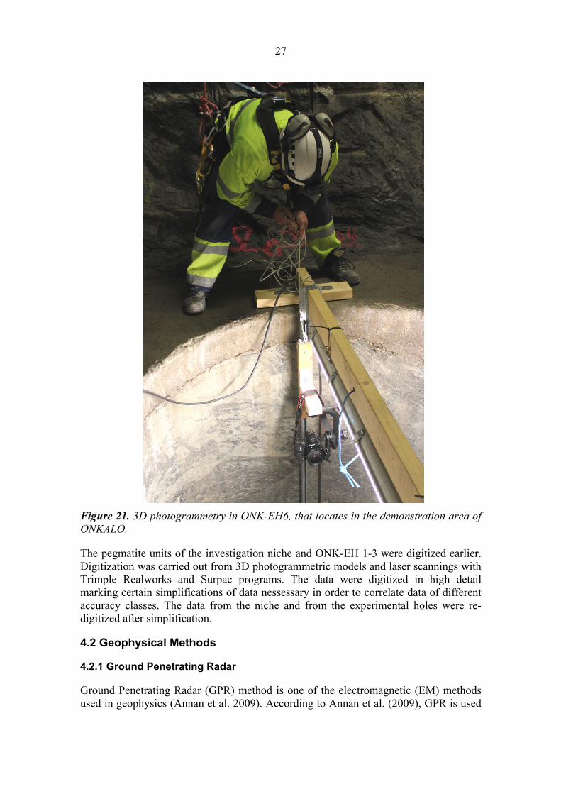
Posiva Oy uses 3D photogrammetry also in the modeling and mapping of the test holes with a method that was developed by Johanna Savunen and Juha Heine. The repository holes are photographed from all cardinal points (north, west, south and east). The equipment and the photogrammetry method are presented in Figure 21. Experimental holes 1, 2 and 3 were photographed during the summer of 2013.
27
Figure 21. 3D photogrammetry in ONK-EH6, that locates in the demonstration area of ONKALO.
The pegmatite units of the investigation niche and ONK-EH 1-3 were digitized earlier. Digitization was carried out from 3D photogrammetric models and laser scannings with Trimple Realworks and Surpac programs. The data were digitized in high detail marking certain simplifications of data nessessary in order to correlate data of different accuracy classes. The data from the niche and from the experimental holes were re-digitized after simplification.
4.2 Geophysical Methods
4.2.1 Ground Penetrating Radar
Ground Penetrating Radar (GPR) method is one of the electromagnetic (EM) methods used in geophysics (Annan et al. 2009). According to Annan et al. (2009), GPR is used

28
in geophysical consulting, geotechnics, sedimentology, glaciology and archaeology. During the GPR measurement short pulses of waves are created with the radar antenna transmitter and a receiver antenna records the amplitude of the returning energy with respect of time (Heikkinen et al. 2011, Musset et al. 2000).
When studying soil with GPR, the possible theoretical amplitudes are between 10-10000 MHz, but the used range is usually between 25-1000 MHz (Annan et al. 2009, Musset et al. 2000). High frequency gives a specific picture but the penetration depth is only a few meters. Even at the lowest frequencies, the penetration depth is limited to a few tens of meters (Musset et al. 2000). Also even a thin layer of clay or presence of salt in the ground-water blocks penetration effectively (Annan et al. 2009).
When GPR is used to characterize near surface features, the used amplitudes are usually over 1 GHz. In that case the penetration depth is around 1 m. While using traditional GPR units with lower frequencies the penetration depth is less than 20 m.
The speed in the ground depends on the dielectric constant, Ԑr which varies depending on the penetrating material (Musset et al. 2000). The penetration depth can be calculated with the following equation,
√
(3)
where twt is a bidirectional delay, c is the velocity of light and er is dielectricity (Daniels et al. 2004).
GPR lines from the floor of the investigation niche were measured during the years 2009-2013. The measurements have been carried out with SIR-300 GPR unit, manufactured by Geophysical Survey Systems, Inc. There are 9 GPR lines parallel to the niche and 14 lines transverse to the niche. The layouts of the lines are represented in Figures 22, 23, and 24.

29
Figure 22. GPR sections parallel to the niche. Interpretations of possible reflectors are shown as red, blue and yellow dashed lines. Interpretations were carried out by Pekka Kantia (Geofcon).
Figure 23. 270MHz transverse GPR sections of the niche.
30
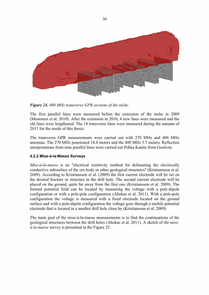
Figure 24. 400 MHz transverse GPR sections of the niche.
The first parallel lines were measured before the extension of the niche in 2009 (Mustonen et al. 2010). After the extension in 2010, 4 new lines were measured and the old lines were lengthened. The 14 transverse lines were measured during the autumn of 2013 for the needs of this thesis.
The transverse GPR measurements were carried out with 270 MHz and 400 MHz antennas. The 270 MHz penetrated 14.4 meters and the 400 MHz 5.7 meters. Reflection interpretations from nine parallel lines were carried out Pekka Kantia from Geofcon.
4.2.2 Mise-á-la-Masse Surveys
Mise-á-la-masse is an "electrical resistivity method for delineating the electrically conductive subsurface of the ore body or other geological structures" (Kristiansson et al. 2009). According to Kristiansson et al. (2009) the first current electrode will be set on the desired fracture or structure in the drill hole. The second current electrode will be placed on the ground, quite far away from the first one (Kristiansson et al. 2009). The formed potential field can be located by measuring the voltage with a pole-dipole configuration or with a pole-pole configuration (Ahokas et al. 2011). With a pole-pole configuration the voltage is measured with a fixed electrode located on the ground surface and with a pole-dipole configuration the voltage goes through a mobile potential electrode that is located in a another drill hole close by (Kristiansson et al. 2009).
The main goal of the mise-á-la-masse measurements is to find the continuations of the geological structures between the drill holes (Ahokas et al. 2011). A sketch of the mise-á-la-masse survey is presented in the Figure 25.

31
Figure 25. Mise-á-la-masse measurement between two drill holes (Ahokas et al. 2011).
Posiva Oy has developed mise-á-la-masse measurement electrodes (Figure 26). The yellow rubber disks prevent the current from drifting along the drill hole ensuring that the current can be focused on the desired fracture or structure (Ahokas et al. 2011). Resistivity is measured with the Terrameter SAS 1000 device.
Figure 26. Posiva's electrodes for mise-á-la-masse surveys (Ahokas et al. 2011).
Mise-á-la-masse measurements were carried out in drill holes ONK-PP398-405 during the autumn of 2013. This was done before drill holes ONK-PP400-403 were deepened. The measurements were carried out with the pole-pole configuration. An average of ten grounding stations in each drill hole, were applied for current feed. A total of 84 groundings were made. On the wall of the experimental hole 14 bolts were attached into fractures and pyrrhotite bearing VGN zones, which were also used as current stations. The measurements proceeded at 10 cm steps downwards from the top of the drill hole. The current feed in the bolts was measured each time in the three closest drill holes. That way any fracture connections and conductive zones between the drill holes could be detected.

32
After the measurements, a total of 226 possible connections were detected. That is because connections may exist in a straight line along the fracture or conductive zone or they can follow a more complex conductive path in the bedrock. Many of the conductors are also linked together into a larger domain. Connections between groundings and bore holes were assessed on the basis of the potential maximum at the location, where a connection exists (Ahokas et al. 2011). According to Ahokas et al. (2011), a clear maximum preferably at a different location from the theoretical curve or a profile showing a minimum indicates the case of no connection.
An example of conductive zone can be seen in Appendix 5, where there is a clear anomaly in the current, feeded from bolt 2. The dashed line indicates the calculated current value and the red line is the measured current value. According to Appendix 5, there is a conductive zone in drill holes ONK-PP398-399 and ONK-PP405, but drill hole ONK-PP404 has no connection.
The most prominent conductor occurred at the depth of 4.5-5.5 m. All in all 62 connections were detected in this layer (Figure 27). The zone could be seen in drill holes ONK-PP398-401 and ONK-PP404-405. There was a conductive layer also in some drill holes at the depths of 6-6.5 m and 7.5-8 m. However the drill holes should have been deepened to detect this zone. The conductor paths are visualized in Surpac as strings. This visualization and interpretation of the mise-á-la-masse data was carried out by the geophysicist Eero Heikkinen from Pöyry Finland Oy.

33
Figure 27. Conductors detected by mise-á-la-masse measurements. Red colour indicates pegmatite granite and blue indicates veined gneiss. View to east.
4.2.3 Drill Hole Geophysics
The goal of the borehole logging, also called geophysical borehole logging (Heikkinen et al. 2011), is to provide data describing the rock mass from the drill holes. Proved features include anomalous zones, continuity and orientation of the fractures and rock mass quality (Posiva 2011). Rock mass has some typical average levels of parameters. If the measured value differs from these levels, it is called an anomaly. Borehole logging describes a 10-30 cm range around the drill hole.
34
Drill hole geophysics are also used at the mining industry. For example the McCreary and Wänsted (1994) described how the drill hole geophysics was used to define the ore sulphide from the waste sulphide.
Raw measurement data initially consist of various voltage, current or count rate values depending on the measured parameters and the tool technique. In this case the measured features are gamma-gamma density (gcm-3), natural gamma radiation (uR/h), magnetic susceptibility (1E-5), full waveform sonic (m/s), focused resistivity (ohmm), optical borehole imaging (OBI), acoustic bore hole imaging (ABI or UBI) and borehole radar (Heikkinen et al. 2011). The parameters are measured with various techniques. Density is measured on the basis of back scattering of gamma radiation from a Cs-37 source of known intensity (Öhman et al. 2009). Natural gamma radiation is measured using semiconductor crystal sensitive gamma rays. Susceptibility is measured using a low frequency electromagnetic induction tool. Full waveform sonic is measured by detecting the acoustic wave transmission time from a pietzoelectric transducer to a similar receiver (Öhman et al. 2009). Resistivity is measured with a four-electrode probe with the electrical current injected into the bedrock with two electrodes while two other electrodes are used to measure the electrical potential (Palmén et al. 2005). Poisson's ratio, Young's modulus and Bulk moduli are rock mechanical parameters which dynamic values can be estimated together with density and velocities (Öhman et al. 2009).
Density describes the mineral composition of the rock mass. Elevated iron content, biotite, amphiboles mafic gneiss, mica gneiss or quartz gneiss inclusions may increase the density values (Öhman et al. 2009). According to Öhman et al. (2009), significant fractures may indicate lower density due to an increase in water content and washout in the fracture. Susceptibility can be diamagnetic (graphite), paramagnetic (silica minerals) or ferrimagnetic (magnetite, pyrrhotite or ilmenite) (Heikkinen et al. 2011). Exceptionally high values indicate the presence of magnetite. Gamma radiation is mostly associated with radioactive potassium 40-K or it's daughter isotopes bearing silica minerals. Low values indicate mafic inclusions and high K-rich minerals. High resistivity values are good measures of the intensity of brittle deformation because the porosity of the rock causes resistivity anomalies (Palmén et al. 2005). Velocities are usually linked to mineralogy and texture (Öhman et al. 2009).
Heikkinen et al. (2011) have also defined the typical fracture characteristics for all of the preceding geophysical features. Resistivity changes usually indicate the presence of water, clay, sulphide or graphite in the fracture filling. Variation in susceptibility indicates a magnetic or graphite filling. Density change indicates water, clay or grain filling fractures and seismic velocities fluctuate because of mechanical discontinuity, presence of water or a clear mineral filling (Heikkinen et al. 2011).
Drill hole geophysics is a vital tool for drill core logging. When the drill core is too broken to be orientated, fractures can be seen either in the optical borehole image (OBI) or in the acoustic borehole image (ABI) and the fracture orientations can be defined (Posiva Oy 2011). As a part of this thesis the fractures were logged from ONK-PP398-405 and ONK-PP410-413 on the basis of optical and acoustic borehole images with the WellCad program. An example of drill hole geophysics and fracture logging of images is presented in Appendix 4. Similar Tables exist of all the preceding drill holes.

35
Similar full scale geophysics has been applied to drill cores ONK-PP199-200, ONK-PP226, ONK-PP398-405 and ONK-PP410-413. In addition to this, optical and acoustic borehole imaging has carried out on several drill cores from the niche. For the modeling, only ONK-PP398-405 and ONK-PP410-413 were taken into account. The geophysical interpretations of the physical features of the rock (Appendix 8.) was carried out by Eero Heikkinen (Pöyry Finland Oy) based on the borehole data.
4.3 3D-modeling Methods
The geological 3D modeling method depends mainly on the modeled features and the modeled area. Numerical methods are widely used when there is a need to convert 2D data into 3D. For example Wu et al. (2004) proposed a modeling method called "-3D modeling with multi-source data intergration". Wu et al. (2004) combined topography data, drill core data and various geophysical data and created numerical algorithms. These algorithms were displayed as a mesh and combined with the modeled structure planes. Using several 2D and 3D modeling programs crosswise, this allowed Wu et al. (2004) created a 3D model of one of their study areas.
In ore body modeling, it is typical to model so called cutting profiles. This method is used, for example, in Rantala's (2011) Master of Thesis. He modeled Hammaslahti's ore by creating 67 cutting profiles at every 25 meters (Rantala 2011). When these cutting profiles were combined, the ore could be modeled as one solid (Rantala 2011). This method works well, if the modeled area is large and the available data supports it.
The main goal this Master of Science Thesis was to create a geological model for the needs of a rock mechanical back-analysis. The main goal of modeling was to combine diverse data from different sources and to produce a geological model that corresponds to the geology of the niche and its surroundings as well as possible. For that reason, it was important to create specific models for the three geological features that can have an effect on the behavior of the rock. These features are lithology, fractures and foliation. Drill hole geophysics also provided information on physically anomalous zones or features in the area of the niche. These features were modeled, because they might have effects on the mechanical behavior of the rock.
During the modeling process, the lithological model was divided into five components. First, the detailed models were created of the ONK-EH1-3, the EDZ-field and the surface of the niche. After that the detailed models were combined with the help of geophysics. In the modeling of the ground penetrating radar reflections, the cutting plane technique was utilized. The reflectors were digitized from every draped GPR -line and the combined reflector lines were interpreted with the detailed lithological models. After that, a 3D block was created around the investigation niche. This block was then filled with the lithological features by following the already modeled unit continuations (direction and dip) and predominant foliation.
The foliation and fractures were modeled as discs and physical rock properties were modeled as individual sections. If mise-á-la-masse measurements or ground penetrating radars provided information about continuations of the fractures or fracture sets, this information was taken into account during modeling.
36
The data used in modeling are presented in Chapters 4.1 and 4.2. Various other geophysical measurements have also been carried out in the EDZ-field. Seismic reflection, seismic tomography and flow log measurements can be mentioned as examples (Mustonen et al. 2009). However, it was not possible to use all the available data in modeling because of the limited time range.
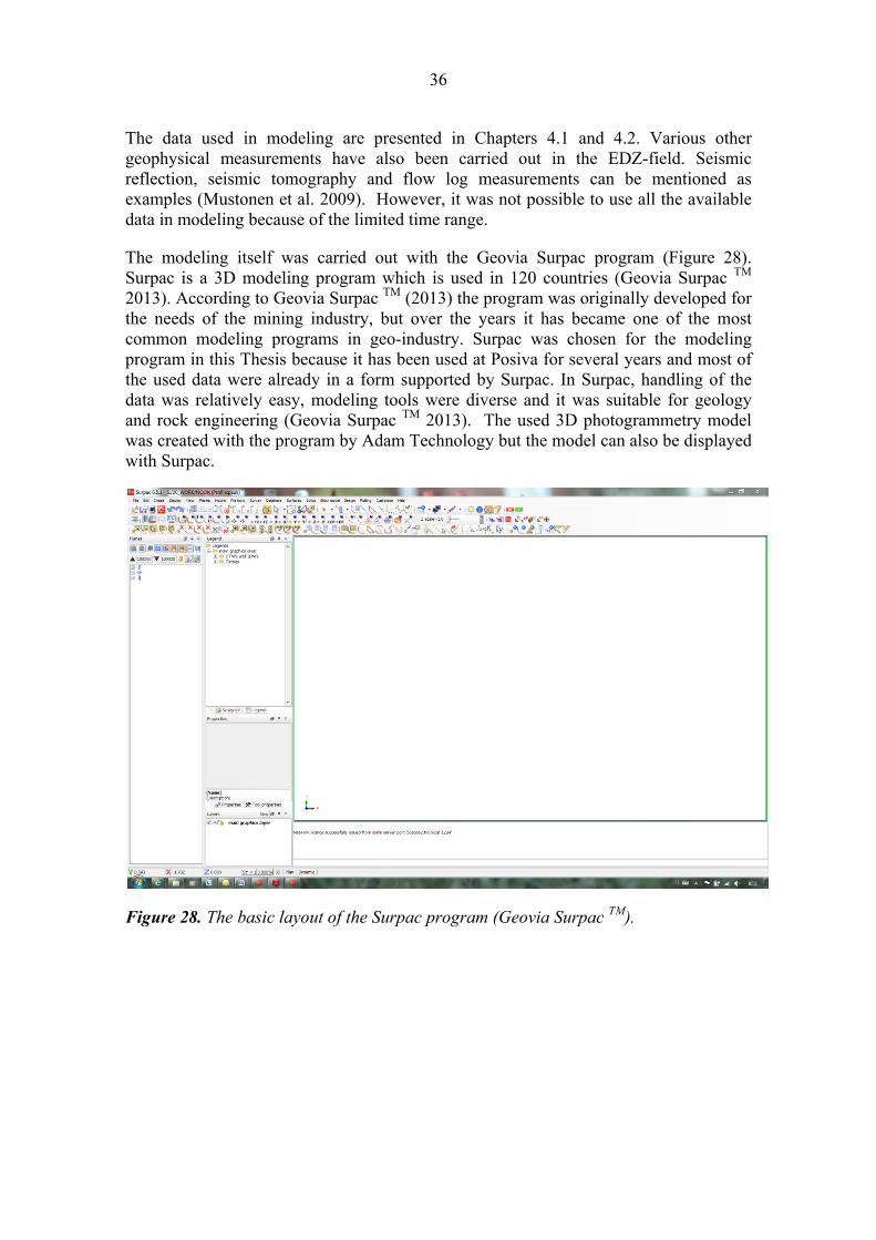
The modeling itself was carried out with the Geovia Surpac program (Figure 28). Surpac is a 3D modeling program which is used in 120 countries (Geovia Surpac TM 2013). According to Geovia Surpac TM (2013) the program was originally developed for the needs of the mining industry, but over the years it has became one of the most common modeling programs in geo-industry. Surpac was chosen for the modeling program in this Thesis because it has been used at Posiva for several years and most of the used data were already in a form supported by Surpac. In Surpac, handling of the data was relatively easy, modeling tools were diverse and it was suitable for geology and rock engineering (Geovia Surpac TM 2013). The used 3D photogrammetry model was created with the program by Adam Technology but the model can also be displayed with Surpac.
Figure 28. The basic layout of the Surpac program (Geovia Surpac TM).
37
5. RESULTS
5.1 Lithological Model
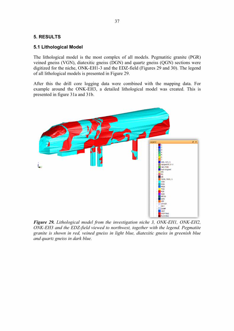
The lithological model is the most complex of all models. Pegmatitic granite (PGR) veined gneiss (VGN), diatexitic gneiss (DGN) and quartz gneiss (QGN) sections were digitized for the niche, ONK-EH1-3 and the EDZ-field (Figures 29 and 30). The legend of all lithological models is presented in Figure 29.
After this the drill core logging data were combined with the mapping data. For example around the ONK-EH3, a detailed lithological model was created. This is presented in figure 31a and 31b.
Figure 29. Lithological model from the investigation niche 3, ONK-EH1, ONK-EH2, ONK-EH3 and the EDZ-field viewed to northwest, together with the legend. Pegmatite granite is shown in red, veined gneiss in light blue, diatexitic gneiss in greenish blue and quartz gneiss in dark blue.
38
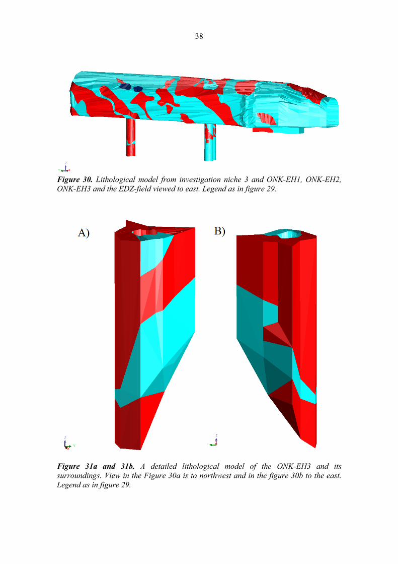
Figure 30. Lithological model from investigation niche 3 and ONK-EH1, ONK-EH2, ONK-EH3 and the EDZ-field viewed to east. Legend as in figure 29.
Figure 31a and 31b. A detailed lithological model of the ONK-EH3 and its surroundings. View in the Figure 30a is to northwest and in the figure 30b to the east. Legend as in figure 29.

39
I tried to use the same technique around the ONK-EH1 and 2 but the geology was too complex to be interpreted only with the drill core data. In this situation, the PGR units from the experiment holes were combined, the floor of the niche and the drill cores and then the ground penetrating radar data was used. The GPR data showed continuations of the PGR units, which made the integration of the experimental hole mapping data and tunnel mapping data possible (Figures 32 and 33). This technique also worked well for the modeling of the EDZ-field. The lithological model of the EDZ-field can be seen in Figure 34.
Figure 32. The continuations of the PGR units around ONK-EH1 and 2 viewed to west. Legend as in Figure 29.
Figure 33. The continuations of the PGR units around ONK-EH1 and 2 viewed to east. Legend as in Figure 29.

40
Figure 34. The lithological model of the EDZ-field viewed to the northwest. Legend as in Figure 29.
Lithological units that did not seem to have any continuations in the data were modeled as lenses. A good example of this can be seen in Figure 30 where QGN units are modeled as dark blue lenses on the west wall of the niche. A second example is provided in Figure 33, where the PGR lens is attached to the west wall of ONK-EH2.
To enable rock mechanical modeling, the lithological model was extended to certain boundary conditions. An imaginary 3D block was created according to these conditions. The corner coordinates of the block are presented in Table 1. The block can be seen in Figure 35. The dimensions of the block were extended beneath ONK-EH3 because some of the drill cores around the experimental hole were 13 m deep.
Table 1. The corner coordinates of the 3D block.
y-coordinate x-coordinate z-coordinate6792348 1525456 -3366792298 1525456 -3366792348 1525470 -3366792348 1525470 -3586792298 1525470 -3366792348 1525456 -352.56792298 1525470 -352.56792298 1525456 -352.5
6792329.25 1525470 -352.56792329.25 1525456 352.56792329.25 1525470 -3586792329.25 1525456 -358
41
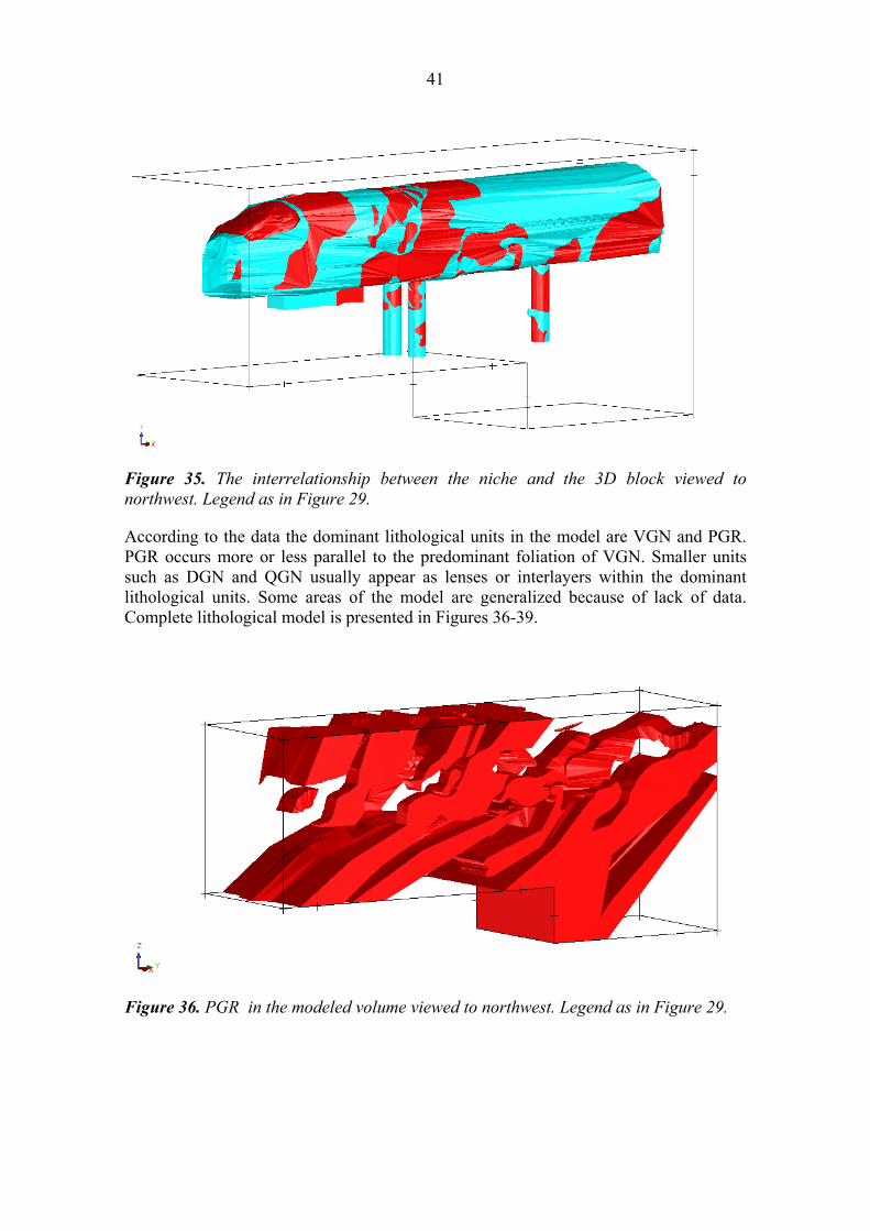
Figure 35. The interrelationship between the niche and the 3D block viewed to northwest. Legend as in Figure 29.
According to the data the dominant lithological units in the model are VGN and PGR. PGR occurs more or less parallel to the predominant foliation of VGN. Smaller units such as DGN and QGN usually appear as lenses or interlayers within the dominant lithological units. Some areas of the model are generalized because of lack of data. Complete lithological model is presented in Figures 36-39.
Figure 36. PGR in the modeled volume viewed to northwest. Legend as in Figure 29.

42
Figure 37. VGN and DGN in the modeled volume viewed to northeast. Legend as in Figure 29.
Figure 38. The lithological model of the modeled volume viewed to northwest. Legend as in Figure 29.

43
Figure 39. The litological model of the modeled volume viewed to northeast. Legend as in Figure 29.
5.1.1 Modeled mica bands
During the POSE experiment, most of the damage occurred in the veined gneiss, where mica content is high. These mica bearing sections also occur at some parts or the pegmatite granite. For that reason, it was also important to model the mica bands within the PGR. These mica bands could be seen at the wall of experimental hole 3 and in some drill cores around it. These bands were firstly digitized as strings and then these strings were connected to the locations in the drill cores, where similar type of bands occur. The modeled mica bands are presented in Figures 40a and 40b.

44
Figure 40a and 40b. The mica bandss around the ONK-EH3. 40a viewed to east and 40b viewed to west.
5.2 Foliation Model
The foliation model was created from the foliation measurements carried out during the systematic geological mapping of the niche and during drill core loggings. Some foliation measurements were also made on the optical borehole images of the drill holes. The foliations are modeled as purple discs with a diameter of 3 m. Modeled foliation measurements are presented in Appendix 6. In Figures 41 and 42 present, the foliation discs with the layout of the niche.

45
Figure 41. Foliation discs with the layout of the niche viewed to northwest.
Figure 42. Foliation discs with the layout of the niche viewed to northeast.
All the foliation measurements were made on VGN and DGN. For that reason it is logical to compare the foliation model and the lithological model of veined and diatexitic gneiss to each other. This is presented in Figure 43.

46
Figure 43. Foliation discs in comparison to the modeled VGN lithology viewed to northwest. Legend as in Figure 29.
Foliation data was also plotted in the Rocscience Dips program which is a stereonet analysis program designed for an interactive analysis of orientation based geological data (Figure 44). The mean value for the main foliation orientation is 164/46, which is similar to the general foliation orientation of Olkiluoto bedrock (Posiva 2011). Another more uncommon foliation orientation is also visible and with the mean orientation 62/39 (dir/dip). These two foliation directions can also be seen in the foliation model.
Figure 44. Foliation measurements plotted in stereonet.
47
5.3 Fracture Model
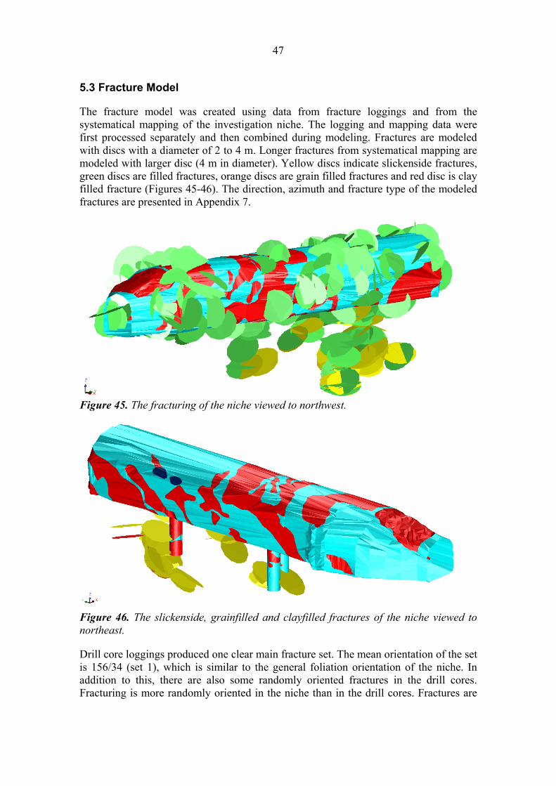
The fracture model was created using data from fracture loggings and from the systematical mapping of the investigation niche. The logging and mapping data were first processed separately and then combined during modeling. Fractures are modeled with discs with a diameter of 2 to 4 m. Longer fractures from systematical mapping are modeled with larger disc (4 m in diameter). Yellow discs indicate slickenside fractures, green discs are filled fractures, orange discs are grain filled fractures and red disc is clay filled fracture (Figures 45-46). The direction, azimuth and fracture type of the modeled fractures are presented in Appendix 7.
Figure 45. The fracturing of the niche viewed to northwest.
Figure 46. The slickenside, grainfilled and clayfilled fractures of the niche viewed to northeast.
Drill core loggings produced one clear main fracture set. The mean orientation of the set is 156/34 (set 1), which is similar to the general foliation orientation of the niche. In addition to this, there are also some randomly oriented fractures in the drill cores. Fracturing is more randomly oriented in the niche than in the drill cores. Fractures are

48
presented in a pole plot and in a contour plot. In the contour plot, two fracture sets, in addition to main fracture set, stand out. The mean orientations of these two sets are 270/85 (set 2) and 342/83 (set 3) (Figure 47).
Figure 47. Fracture orientations (set 1-3) with pole plot on the left and contour plot on the right.
5.4 Physical Rock Property Model
The modeled anomalous zones are marked in the borehole logging table (Appendix 4). For the needs of rock mechanics, physically anomalious rock property zones were modeled. The clearly observable differences in densities, seismic velocities, Poisson's ratios and Young's modulus were taken into account.
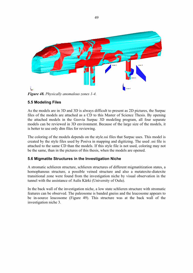
In total four anomalous physical rock property zones were distinguished from VGN and DNG (Figure 48). In zone 1, seismic velocities, Young's modulus and shear modulus are lowered. In zone 2, density is average, susceptibility is ferrimagnetic, resistivity is conductive, seismic velocities are lowered and Young's modulus, shear modulus and Poisson's ratio are lowered. In zone 3, density is elevated, susceptibility is elevated (ferrimagnetic), resistivity is lowered or conductive, seismic velocities are low, Young's modulus and shear modulus are lowered and Poisson's ratio is average. In zone 4, density varies from low to average, susceptibility is ferrimagnetic, resistivity is conductive, seismic velocities are lowered and Young's modulus, shear modulus and Poisson's ratio are clearly lowered.
49
Figure 48. Physically anomalous zones 1-4.
5.5 Modeling Files
As the models are in 3D and 3D is always difficult to present as 2D pictures, the Surpac files of the models are attached as a CD to this Master of Science Thesis. By opening the attached models in the Geovia Surpac 3D modeling program, all four separate models can be reviewed in 3D environment. Because of the large size of the models, it is better to use only dtm files for reviewing.
The coloring of the models depends on the style.ssi files that Surpac uses. This model is created by the style files used by Posiva in mapping and digitizing. The used .ssi file is attached to the same CD than the models. If this style file is not used, coloring may not be the same, than in the pictures of this thesis, when the models are opened.
5.6 Migmatite Structures in the Investigation Niche
A stromatic schlieren structure, schlieren structures of different migmatitization states, a homophanous structure, a possible veined structure and also a metatexite-diatexite transitional zone were found from the investigation niche by visual observation in the tunnel with the assistance of Aulis Kärki (University of Oulu).
In the back wall of the investigation niche, a low state schlieren structure with stromatic features can be observed. The paleosome is banded gneiss and the leucosome appears to be in-source leucosome (Figure 49). This structure was at the back wall of the investigation niche 3.

50
Figure 49. The low state schlieren structure.
In the both back corners of the niche could be observed a metatexitic schlieren structure. The metatexitic schlieren (figure 50) appear to be located on the transitional zones between the big leucosome and paleosome units. The leucosome content can vary in this structure.
Figure 50. The metatexitic schlieren structure.

51
The third migmatite structure is located on the east wall of the niche, close to the experimental hole 3. This structure is clear deformated metatexditic schlieren (Figure 51). The rock is melanocratic and the paleosome is close to a flame shape.
Figure 51. The deformated metatexitic schlieren structure.
The fourth structure is a diatexite that consists of homophanous (Figure 52) and sclieren components (Figures 49-51). The observed melt is anatexitic and the first melt has left the current material in an early stage. If the melting had proceeded further, the formed rock type would have been granodiorite.
Figure 52. The homophanous structure.

52
The fifth migmatite structure type is a possible veined structure. It could not be fully confirmed with visual inspection that the visible white leucosome parts continue as veins further in the bedrock. However the leucosome indicate further continuation. The structure can be seen in the east wall of ONK-EH3 (Figure 53).
Figure 32. The veined structure in experimental hole 3.
Otherwise migmatite structures were repeated in the area of the niche. One additional transitional zone was found, where the metatexitic migmatite turns gradually into diatexitic migmatite (Figure 54) from right to left respectively. The transition occurs gradually in the marked area. For comparison the observed paleosome of the diatexite is presented in Figure 55.
Figure 54. The transition from the metatexite to diatexite.

53
Figure 55. The paleosome of the diatexitic migmatite.

54
55
6. DISCUSSION
6.1 Applicability and Representativeness of the Data and Methods
There were several geological and geophysical data sets available from the study area. The main emphasis was on the systematical mapping and drill core logging data sets. These formed the base for modeling. Geophysical data was used for supporting data. Geophysical data enabled the expansion of the model to areas where direct geological information was limited or lacking.
The ground penetrating radar is a fast and cost effective method and most usable in a situation where the studied structure can be observed, for example, on the floor of the niche or in the drill core (Mustonen et al. 2010). Observation provides a possibility to follow this structure further in the bedrock. However, if the reflector cannot be seen at the study area, the interpretation is difficult. In this study, GPR gave good and strong reflections at the lithological boundaries, especially if they were close to the floor of the niche. With this data it was possible to extend the lithological units deeper into the bedrock and supplement the imaginary 3D block.
The GPR data was also integrated into the drill core logging data. Ground penetrating radar gave reflection to the known lithological boundaries and at some fractures. However, the dip angle was a little bit smaller than the dip angle of the structure in the drill core. GPR lines parallel to the niche were extremely good, but unfortunately the mesh on the roof of the niche produced so much disturbance to the parallel lines that it was almost impossible to detect the real reflections on the reflection image.
Mise-á-la-masse measurements were mostly used for the integration of fracture data between the drill holes. The main goal of mise-á-la-masse measurements was to provide more information about the slickenside fracture set located under ONK-EH3. Unfortunately the measurements were carried out before the drill holes were deepened and for that reason the mise-á-la-masse measurements only responded to the second more intensely fractured set at the depth of 4.5-5.5 m around ONK-EH3.
Drill hole geophysical measurements played a significant role in the foliation, fracture and physical rock property models. Fracture loggings were carried out with the optical and acoustical images using the WellCad program, because most of the drill cores could not be oriented to north and logged straight from the core. The anomalous rock's physical properties were also only modeled based on drill hole geophysical measurements.
The modeling method that was used is described in Chapter 4.3. By implementing modeling in smaller individual sections gave a possibility to focus on to even small scale structures. Areas with a higher amount of specific data were modeled in more detail than areas with less data. This modeling method was used in order to minimize the risk of errors. After all the individual sections had been modeled, they were integrated together.
56
6.2 Representativeness of the Model
It became evident during modeling that there was a need for the lithological model to be simplified to some extent. This was because of two reasons. First, there were different accuracy classes in the data sets depending on the location in the niche and simplifications needed to be made to integrate the variable sections. Second, there is a limit to the complexity of the model that can be used in the rock mechanical back analysis. For example, the digitization of the niche and ONK-EH1-3 was very accurate. In contrast to this, the data from drill core loggings and the ground penetrating radar were much more inaccurate. The lithological model is the most accurate around the EDZ-field, close to ONK-EH1 and 2 and around ONK-EH3. The level of accuracy is reduced as the model reaches the faces, edges and corners of the 3D block.
Modeling also involved some interpretations because of the lack of data on some locations. For example, it was possible to create an exceptionally complicated lithological model around ONK-EH1 and 2 because of the high amount of data, but when areas with less data were modeled, certain amount of interpretation had to done. The amount of interpretation could have been minimized with more drillings around the experimental holes. This would have provided the required information for the lithological continuations. For example in ONK-EH2 one pegmatite unit was modeled as a lens although there is a possibility that it might continue deeper down into the bedrock. Some interpretation was also involved in lithological modeling under the EDZ-field. Also in this case the deeper drill cores would have provided the required information.
Foliation model is very accurate. Foliation measurements in the niche are modeled in situ by coordinates and most of the foliation measurements in the drill cores were carried out on optical borehole images. The foliation model produced two sets, a primary and a secondary set. The mean direction is 164/46 for the primary set and 62/39 for the secondary. The orientation of the primary set is close to the general foliation direction in Olkiluoto (Posiva Oy 2011). That explains why this set is more dominant in the measurements.
Fracturing model is also very accurate. Most of the drill core fractures are oriented with optical and acoustical bore hole images and mapping data is modeled in situ by coordinates. Fractures formed 3 sets with the following mean directions: 156/34 (set 1), 270/85 (set 2) and 342/83 (set 3). In set 1, fractures are generally parallel to the foliation and almost all the fractures are logged from the drill cores. Sets 2 and 3 are formed from the results of systematical mapping. Also irregular fracturing occurs. With mise-á-la-masse data it was possible to connect fractures between individual drill holes. Unfortunately the measurements did not provide any information about the slickenside fracture set under experimental hole 3.
Physical rock property model is also as accurate as possible. Borehole logging measures the rock's features ca. 10-30 cm around the bore hole. The zones between the drill holes could be connected that way. When comparing geophysical results and the geology of drill cores, some interpretation of the reasons for the physical anomalies could be done.

57
Physical anomalies in zones 2 and 4 are most likely associated with the slickenside fracturing. This fracturing is addressed more closely in Chapter 6.3. Zones 2 and 4 are located in the same lithological veined gneiss unit, where also intensive fracturing occurs. Core loggings support the bore hole logging data because the zones include graphite, porosity is above average and some pyrrhotite may occur. In zone 1, the gneiss contains a lot of mica and some parts of it could be logged as mica gneiss. Leucosome was also spotted. These features may explain the geophysical anomalies. In zone 3 kaolinization occurs and some porosity is caused by fractures. That explains the anomalies in susceptibility and seismic velocities. Gneiss contains in a noticeable degree of biotite, which cause the increased density.
The most accurate area in the models is the surroundings of ONK-EH3. The several drilling operations as well as drill hole geophysics and the mise-á-la-masse made it possible to create a very specific and detailed model around the experimental hole for all the modeling disciplines. This provided a good benchmark for the work a point from which it was practical to start the expansion process of the model.
All the models are as representative as it was possible to generate with the available data. There are areas where a significant amount of interpretation is involved in the models, but the models are all quite simple to update if new drilling operations or other measurements provide new information about the geology of the niche. The main purpose of this thesis was to provide initial data for the rock mechanical back-analysis and so all the features that may have an effect on the mechanical behavior of the rock were modeled as specifically as possible.
6.3 Correlation with the Site Model
It was clear that investigation niche 3 is one of the least fractured areas in ONKALO. However eight new drill cores (ONK-PP398-405) were drilled around the experimental hole 3 during the summer of 2013. During the logging of these drill cores it was noticed that if the drill core penetrates veined gneiss at the depth of around 5.5-8.20 m, a set of a few slickenside fractures can be seen. These fractures are parallel to the dominating foliation (ca. 164/46) and the movement is either reverse or normal. Regardless of this, there are no signs of this structure anywhere in the niche or at the bottom of ONK-EH3.
When going through the drill core logging data, the same slickenside fracture set could be seen in four older drill cores. These are ONK-PP261, ONK-PP340, ONK-PP346 and ONK-PP347. New drill cores ONK-PP410-411 also penetrate the slickenside fracture set. Unfortunately, there is no information of the dip and dip directions of drill cores ONK-PP340 and ONK-PP346. However, slickenside fractures can be seen in drill cores and they are more or less parallel to the foliation. For that reason, it was possible to model the fractures in the same direction as foliation /160-170/40-50). Apart from the slickenside fractures, the fracture section contains two grainfilled fractures and one clayfilled fracture (Appendix 7).
There was no clear reason for the indication of a possible brittle fault zone under the niche. Afterwards it turned out that one brittle fault zone (ONK-BFZ265) was modeled under the niche in the site model. This zone cross-cuts the ONKALO access tunnel at chainage 4125-4175. When the brittle fault zone was modeled on its location, there was
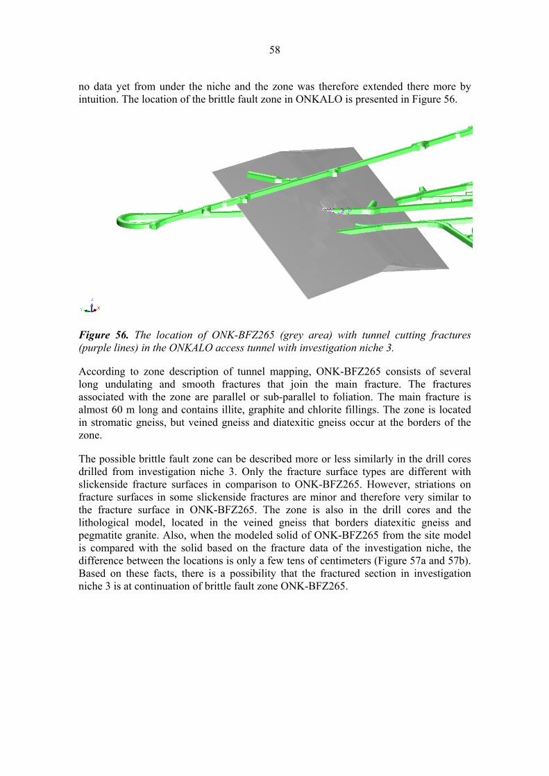
58
no data yet from under the niche and the zone was therefore extended there more by intuition. The location of the brittle fault zone in ONKALO is presented in Figure 56.
Figure 56. The location of ONK-BFZ265 (grey area) with tunnel cutting fractures (purple lines) in the ONKALO access tunnel with investigation niche 3.
According to zone description of tunnel mapping, ONK-BFZ265 consists of several long undulating and smooth fractures that join the main fracture. The fractures associated with the zone are parallel or sub-parallel to foliation. The main fracture is almost 60 m long and contains illite, graphite and chlorite fillings. The zone is located in stromatic gneiss, but veined gneiss and diatexitic gneiss occur at the borders of the zone.
The possible brittle fault zone can be described more or less similarly in the drill cores drilled from investigation niche 3. Only the fracture surface types are different with slickenside fracture surfaces in comparison to ONK-BFZ265. However, striations on fracture surfaces in some slickenside fractures are minor and therefore very similar to the fracture surface in ONK-BFZ265. The zone is also in the drill cores and the lithological model, located in the veined gneiss that borders diatexitic gneiss and pegmatite granite. Also, when the modeled solid of ONK-BFZ265 from the site model is compared with the solid based on the fracture data of the investigation niche, the difference between the locations is only a few tens of centimeters (Figure 57a and 57b). Based on these facts, there is a possibility that the fractured section in investigation niche 3 is at continuation of brittle fault zone ONK-BFZ265.
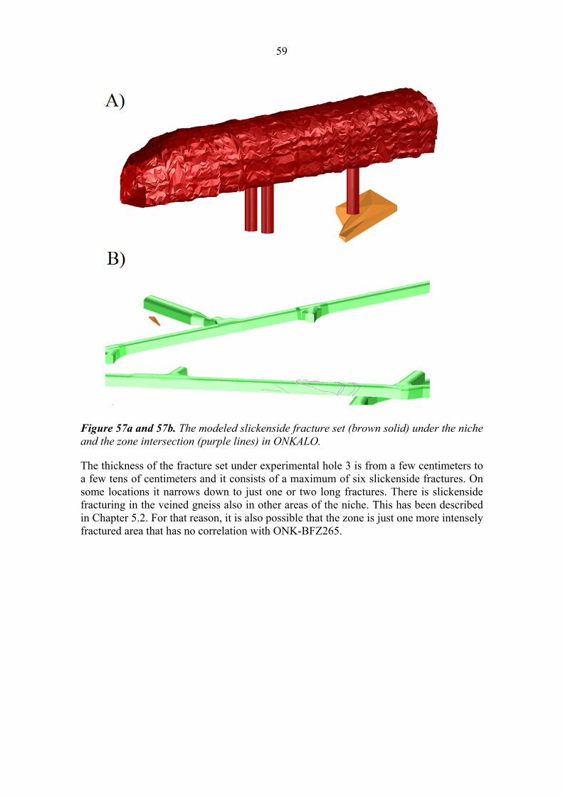
59
Figure 57a and 57b. The modeled slickenside fracture set (brown solid) under the niche and the zone intersection (purple lines) in ONKALO.
The thickness of the fracture set under experimental hole 3 is from a few centimeters to a few tens of centimeters and it consists of a maximum of six slickenside fractures. On some locations it narrows down to just one or two long fractures. There is slickenside fracturing in the veined gneiss also in other areas of the niche. This has been described in Chapter 5.2. For that reason, it is also possible that the zone is just one more intensely fractured area that has no correlation with ONK-BFZ265.

60

61
7. SUMMARY AND CONCLUSIONS
The geological model of investigation niche 3 was created as initial data for a rock mechanical back analysis related to the POSE experiment. The goals of the POSE experiment are to determine the in situ stress conditions and spalling strength of the bedrock as well as to "act as a Prediction-Outcome exercise" (Johansson 2014). Because of the unexpected results of the experiment, a geological model of the niche and its surroundings needed to be created.
In the lithological model the main rock types were veined gneiss and pegmatite granite. Small inclusions of diatexitic gneiss and quartz gneiss occur also in the area. The lithological model is extended to certain boundary conditions defined by rock mechanics. In the foliation model, two different foliation sets occur. The main orientations of these sets are 164/46 (set 1) and 62/39 (set 2). In the fracture model, three different fracture sets occur. The main orientations of the sets are 156/34 (set 1), 270/85 (set 2) and 342/83 (set 3). Set 1 consists mostly of slickenside fractures that may be at continuation of brittle fault zone 265. This is described in Chapters 5.3 and 6.3. In the rock property model, 4 anomalous zones occur near ONK-EH3. Zone descriptions and interpretations are provided in Chapters 5.4 and 6.2.
The geological model of the investigation niche is as accurate as it was possible to make with the data available. However, there are also certain areas in the model where significant interpretation has been carried out because of lack of data. For example, some interpretation is involved in the lithological model around ONK-EH1 and 2 and between ONK-EH1 and 2 and the EDZ-field. If there is a need for the model to be more accurate, it is recommended that further drilling operations will be employed. A proposal of eight new vertical drill cores has been made, as presented in the Figure 58, which would make the model more specific.
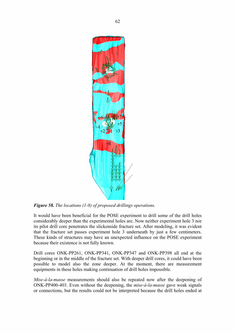
62
Figure 58. The locations (1-8) of proposed drillings operations.
It would have been beneficial for the POSE experiment to drill some of the drill holes considerably deeper than the experimental holes are. Now neither experiment hole 3 nor its pilot drill core penetrates the slickenside fracture set. After modeling, it was evident that the fracture set passes experiment hole 3 underneath by just a few centimeters. These kinds of structures may have an unexpected influence on the POSE experiment because their existence is not fully known.
Drill cores ONK-PP261, ONK-PP341, ONK-PP347 and ONK-PP398 all end at the beginning or in the middle of the fracture set. With deeper drill cores, it could have been possible to model also the zone deeper. At the moment, there are measurement equipments in these holes making continuation of drill holes impossible.
Mise-á-la-masse measurements should also be repeated now after the deepening of ONK-PP400-403. Even without the deepening, the mise-á-la-masse gave weak signals or connections, but the results could not be interpreted because the drill holes ended at

63
the slickenside fracture set. The repetition of the measurements would provide much needed information about the fracture set and its influence zone.
If it needs to be determined, whether the slickenside fracture set is somehow connected with brittle fault zone ONK-BFZ265, further investigations have to be carried out. There distance between the drill hole observations and the tunnel cross-cut of ONK-BFZ265 is a little over 100 m. It could be worthwhile to try a mise-á-la-masse survey between the drill holes and the tunnel cross-cut. Unfortunately, the range of mise-á-la-masse may be too short.

64

65
8. ACKNOWLEDGEMENTS
I am the most grateful to Posiva Oy for giving me this opportunity to write my Master of Science Thesis as part of their POSE project. My supervisors Ismo Aaltonen, Antti Joutsen and Topias Sirén at Posiva and Timo Kilpeläinen at the University of Turku deserve my gratitude. I also want to thank all my co-workers at Posiva Oy for helping me during the writing work of this Thesis. I especially want to thank Jyrki Liimatainen for creating for me the Surpac database for the modeling. I also wish extend to my thanks to geophysicists Eero Heikkinen from Pöyry Finland Oy and Pekka Kantia from Geofcon for providing geophysical data and interpretations to me. Thanks to Jouni Valli from Pöyry Finland Oy for providing me consultation supporting to the project. I also want to thank Aulis Kärki at the University of Oulu for helping me with the migmatite structures of the niche.
Most of all I want to thank my fiancé Ville, my family and all my friends for supporting me through this project and for giving me strength every day.

66
67
9. REFERENCES
Aaltonen I. (ed.), Lahti M., Engström J., Mattila J., Paulamäki S., Gehör S., Kärki A., Ahokas T., Torvela T., Front K. 2010. Geological model of Olkiluoto Site Version 2.0. Posiva Oy. Olkiluoto. Finland. 280p.
ADAM Technology. 2010a. 3DM Analyst Mine Mapping Suite 2.3.4 Users Manual. 3D Measurement, Camera Calibration and Block Adjustment Software. ADAM Technology. Belmont, Australia. 369p.
Adam Technology. 2010b. 3DM Analyst Mine Mapping Suite for underground tunnel mapping and geotechnical applications, Instruction of taking underground photos. ADAM Technology. Belmont, Australia. 3p.
Ahokas T., Heikkinen E., Hurmerinta E. 2011. Mise-á-la-Masse Survey in the HYDCO Niche 2011. Working Report 2011-89. Posiva Oy. Olkiluoto, Finland. 37p.
Andersson J. C. 2007. Äspö Hard Rock Laboratory. Äspö Pillar Stability Experiment, Final report. Rock mass response to coupled mechanical thermal loading. Svensk Kärnbränslehantering AB. Sweden. 207p.
Annan A. E., Cassidy N. J., Koppenjan S., Daniels D. J., Doolittle J. A., Butnor J. R., Slater L., Comas X., Redman J. D., Bristow C., Buynevich I. V., FritzGerald D. M., Bridge J., Arcone S. A., Saarenketo T., Yarovog A., Goodman D., Piro S., Nishimura Y., Schneider K., Hongo H., Higashi N., Steinberg J., Damiata B., Jol H. M. (ed). 2009. Ground Penetrating Radar: Theory and Applications. Elsevier Science. United Kingdom. 507p.
Barton W. R., Lien R., Lunde J. 1974. Engineering Classification of Rock Masses for the Desing of Tunnel Support. Rock Mechanics and Rock Engineering. Springer-Verlag. London, United Kingdom. 47p.
Cal M., Kaiser P. K. 2005. Assessment of excavation damaged zone using a micromechanics model. Tunnel and Underground Space Technology 20 (2005). Geomechanics Research Centre, MIRACO, Laurentian University. Elsevier Ltd. Canada. 10p.
Canon Inc. 2012. Canon EOS 6D, EOS 6D (WG), EOS 6D (N) Käyttöohje. Canon Auropa N. V. Amstelveen, Neatherlands. 404p.
Daniels D. J. (ed.), Abrahamsson S., Bartha M., Scott H. F., Bungey J., Hanninen P., van Overmeeren R. A., van Deen J. K., Tillard S., Fidler J., Wilkinson P. L., Cariou J., Schaber G., Haglars T., Nicollin F. 2004. Ground Penetrating Radar. 2nd Edition. The Institution of Engineering and Technology. United Kingdom. 732p.
Deere D. V., Deere D. W. 1988. The Rock Quality Designation (RQD) Index in Practise. Rock Classification Systems for Engineering Purposes. ASTM. Philadelphia, USA. 8p.
68
Deere D. V., Hendron A. J., Patton F. D. Cording E. J. 1967. Design of Surface and Near-Surface Construction in Rock Failure and Breakage of Rock. Society of Mining Engineers of AIME. New York, USA. 302p.
Enescu N., Cosma C. 2010. EDZ Seismic Investigations in ONKALO, 2009. Factual Report. Working Report 2010-26. Posiva Oy. Olkiluoto, Finland. 107p.
Engström, J. 2014. Geological ductile deformation mapping at the Olkiluoto Site, Eurajoki, SW Finland. Working report 2013-62. Posiva Oy, Olkiluoto, Finland. 67 p.
Gemcom SurpacTM. 2013. Integrated Geology, Recourse Modeling, Mine Planning and Production. Gemcom Software International Inc. Vancouver, Canada. 4p.
Grimstad, E. & Barton, N. 1993. Updating of the Q-System for NMT. Proceedings of the International Symposium on Sprayed Concrete - Modern Use of Wet Mix Sprayed Concrete for Underground Support, Fagernes.Kompen, Opsahl and Berg. Norwegian Concrete Association, Oslo. 66p.
Haapala I. 1977. Pertography and geochemistry of the Eurajoki stock, a rapakivigranite complex with greisen-type mineralization in southwestern Finland. Geological Survey of Finland, Bulletin 286. GTK. Espoo, Finland.
Haapala I., Käyhkönen Y., Lehtinen M., Korsman K., Koistinen T., Luukkonen E. J., Sorjonen-Ward P., Silvennoinen A., Laajoki K., Nironen M., Rämö T., Heikkinen E., Heinonen S., Ravimo I. 2011. Semi-Automated Fracture Classification Procedure Based on Geophysical Drillhole Logging Data. Working Report 2011-88. Posiva Oy. Olkiluoto, Finland. 120p.
Heikkinen E., Kantia P. 2011. Suitability of Ground Penetrating Radar for Locating Large Fractures. Working Report 2011-92. Posiva Oy. Olkiluoto, Finland. 64p.
Hurmerinta E., Sacklen N (ed)., Kosunen P., Pekkanen J., Tarvainen A-M., Toropainen V. 2010. Drillings and Associated Drillhole Measurements of the Investigation Holes in the EDZ Tunnel at Chainage 3620. Working Report 2010-17. Posiva Oy. Olkiluoto, Finland. 150p.
Itasca Consulting Group Inc. 2013. 3DEC (3 Dimensional Distinc Element Code) 5.0 User's Guide. Itasca Consulting Group Inc. Mineapolis, USA. 328p.
Johansson E., Siren T., Hakala M. 2014. POSE experiment: Outcome from the POSE Phase 1 and 2. Working Report 2012-30. Posiva Oy. Olkiluoto, Finland.
Kohonen, J., Pihlaja, P., Kujala, H. & Marmo, J. 1993. Sedimentation of the Jotunian Satakunta sandstone, western Finland. Espoo: Geological Survey of Finland. Bulletin 369. 35p.
Korhonen R. (ed.), Korsman K., Pajunen M., Wenneström M., Elo S., Pirttijärvi M. Huhta P., Räsänen M., Laakso K., Säärvuori H., Jarva J., Poutanen M., Ahoja J., Lipping T., Turunen J., Tuominen J., Pohjola J. 2010. Geotietoa Satakunnasta. GeoPori,

69
GeoSatakunta ja InnoGeo projektien loppuraportti. Tutkimus Raportti 183. Geologian tutkimuskeskus. Espoo, Finland. 193p.
Korja, A., Heikkinen, P. J. 1995. Proterozoic extensional tectonics of the central Fennoscandian Shield: Results from the Baltic and Bothnian Echoes from the Lithosphere experiment. Tectonics 14, Issue 2. 504-517p.
Kristiansson S., Heikkinen P. 2009. Mise-á-la-Masse Measurements in Drillholes OL-KR4, OL-KR30 and OL-KR14-OL-KR18 in Olkiluoto. Working Report 2009-10. Posiva Oy. Olkiluoto, Finland. 239p.
Kärki, A. 2014. Migmatites and migmatite-like rocks of Olkiluoto. Posiva Oy. Olkiluoto, Finland. In press.
Kärki A., Paulamäki S., 2006. Petrology of Olkiluoto. Posiva Report 2006-2. Posiva Oy. Olkiluoto, Finland. 77p.
Laitakari I., Vartiainen H. 1998. Suomen kallioperä: 3000 vuosimiljoonaa. Suomen Geologinen Seura Ry. 375p.
Lehtinen M., Nurmi P. A., Rämö O. T. 2005. Precambrian Geology of Finland. Chapter 1: Overview (Vaasjoki M., Korsman K., Koistinen T.) (p. 3-18). Chapter 11: Paleoproterozoic tectonic evolution (Lahtinen R., Korja A., Nironen M.) (p. 481-520). Elsevier B.V. Netherlands. 699p.
Martin C. D., Read R. S. 1996. Technical Raport of AECL's Mine-by Experiment, Phase 1: Excavation Response (Résumé du rapport technique d'EACL sur l'essai au voisinage de l'excavation, Phase 1: Reaction á l'excavation). Atomic Energy of Canada Limited. Canada. 179p.
Martino J. B., Chandler N. A. 2004. Excavation-induced damage studies at the Underground Research Laboratory. International Journal of Rock Mechanics and Mining Sciences. Volume 41 - Issue 8. Elsevier Ltd. Canada. 14p.
Mattila J. 2006. System of Nomenculare for Rocks in Olkiluoto. Working Report 2006-32. Posiva Oy. Olkiluoto, Finland. 16p.
McCreary R. G., Wänsted S. 1994. Applications of Multivariate Statistics and Pattern Recognition to Geophysical Logging at Norada. Quebec, Canada. 32p.
Mehnert K. R. 1968. Migmatites and the orgin of granitic rocks. Elseviel Pub. Co. Amsterdam, Neatherlands. 393p.
Musset A. E., Khan M. A., 2000. Looking into the Earth: An Introduction to Geological Geophysics. The press syndicate of the University of Cambridge. United Kingdom. 438p.
Mustonen S., Norokallio J., Mellanen S., Lehtimäki T., Heikkinen E. 2010. EDZ09 Project and Related EDZ-studies In Onkalo 2008-2010. Working Report 2010-27. Posiva Oy. Olkiluoto, Finland. 404p.

70
Nordbäck N. 2013. Outcome of the Geological Mapping of the ONKALO Undeground Recearch Facility, Chainage 3116-4986. Working Report 2013-11. Posiva Oy. Olkiluoto, Finland. 106p.
Ojala J. 2003. Kallioperäkartoitus maakuvilla. Maanmittaustieteiden Seuran julkaisu nro. 40. Maanmittaustieteiden päivät 2003. Geologian tutkimuskeskus. Helsinki, Finland. 3p.
Palmén, J. , Heikkinen, E., Vaittinen, T. 2005. Unification of short normal resistivity logging data from borehole KR1 – KR28. Posiva Working Report 2005-60. Posiva Oy. Olkiluoto, Finland. 106p.
Paulamäki S., Paananen M., Elo S. 2002. Structure and Geological Evolution of the Bedrock of Southern Satakunta, SW Finland. Working Report 2002-4. Posiva Oy, Helsinki, Finland. 128p.
Paulamäki S. 2009. Geological setting of the Olkiluoto Investigation site, Eurajoki, SW-Finland. Working Report 2009-53. Posiva Oy. Eurajoki, Finland. 56p.
Posiva Oy. 2011. Olkiluoto Site Description 2011. Posiva 2011-02. Posiva Oy. Olkiluoto, Finland. 1032p.
Rantala E. 2011. Hammaslahden malmi ja sen 3D -mallintaminen. Master of Thesis. Geology and Mineralogy. University of Turku. Turku, Finland 49p.
Sawyer E. 2008. Altas of Migmatite. The Canadian Mineralogist. Special Publication 9. National Research Council Canada. NRC Research Press. Ontario, Canada. 371p.
Sederholm J. J. 1907. On granit och gneiss, deras uppkomst, uppträdande och utbredning inom urbergt I Fennoskandia. Bulletin de la Comission Géologique de Finlande 23. Geologian tutkimuskeskus. Helsinki, Finland. 90p.
Siren T., 2011. Fracture Mechanics Prediction for Posiva’s Olkiluoto Spalling Experiment (POSE). Working Report 2011-23. Posiva Oy. Olkiluoto, Finland. 30p
Suominen, V. 1991. The chronostratigraphy of southwestern Finland with special reference to Postjotnian and Subjotnian diabases. Espoo: Geological Survey of Finland. Bulletin 356, 100p.
Suominen, V., Fagerström, P. & Torssonen, M. 1997. Pre-Quaternary rocks of the Rauma map-sheet area (in Finnish with an English summary). Espoo: Geological Survey of Finland. Geological map of Finland 1:100 000: explanation to the maps of Pre-Quaternary rocks, sheet 1132 Rauma, 54p.
Toropainen V. 2008. Core Drilling of Deep Drillhole OL-KR49 at Olkiluoto in Eurajoki 2008. Working Report 2008-80. Posiva Oy. Olkiluoto, Finland. 186p.
Toropainen V. 2010. ONKALO Pose Experiment- Core Drillingf of Drillholes ONK-PP223-226, ONK-PP253-261 and ONK-PP268-271 in ONKALO at Olkiluoto 2009-2010. Working Report 2010-78. Posiva Oy. Olkiluoto, Finland. 66p.

71
Tsang C-F., Bernier F., Davies C. 2005. Geohydromechanical process in the Excavation Damage Zone in crystalline rock, rock-salt and indurated and plastic clays - in the context of radioactive waste disposal. International Journal of Rock Mechanics and Mining Science. Volume 41 - Issue 1. Elsevier Ltd. Belgium. 17p.
Vaasjoki, M. 1996. The Laitila rapakivi batholith revisited: new, more precise radiometric ages. In: Haapala, 1., Rämö, 0. T. & Kosunen, P. (ed.) The Seventh International Symposium on Rapakivi Granites and Related Rocks, Wednesday 24 - Friday 26 July, 1996, University of Helsinki, Helsinki - Finland: abstract volume. Helsinki: University Press, p. 82.
Valli J., Hakala M. 2012. ONKALO POSE experiment – Phase 3: 3DEC prediction. Working Report 2012-58. Posiva Oy, Olkiluoto, Finland. 66p.
Valli J., Hakala M., Wanne T., Kantia P., Siren T. 2011. ONKALO POSE experiment – Phase 3: Execution and monitoring. Working Report 2012-41. Posiva Oy. Olkiluoto, Finland. 163p.
Veräjämäki, A. 1998. Pre-Quaternary rocks of the Kokemäki map-sheet area (in Finnish with an English abstract). Espoo: Geological Survey of Finland. Geological map of Finland 1:100 000, explanation to the maps of pre-Quatemary rocks, sheet 1134 Kokemäki, Finland. 51p.
Wu Q., Xu H., Zou X. 2004. An effective method for 3D geological modeling with multi-source data intergration. Computers and Geosciences (2005). Volume 30, Issue 1. Elsevier Ltd. China. 9p.
Öhman, I., Palmén, J., Heikkinen, E. 2009. Unification of Acoustic Drillhole Logging Data. Working Report 2009-32. Posiva Oy. Olkiluoto, Finland. 64p.

72

AP
PE
ND
IX 1
. An
exam
ple
of th
e dr
ill c
ore
logg
ing
shee
t (O
NK
-PP
405)
Lit
holo
gy
Fol
iati
on
HO
LE_I
DM
_FR
OM
M_T
OR
OC
K_T
YP
ELE
UC
OS
OM
E %
DE
SC
RIP
TIO
Nm
mO
NK
-PP
405
0.00
0.46
CO
NC
RE
TETh
e fir
st 4
6 cm
in c
oncr
ete.
ON
K-P
P40
50.
464.
00P
GR
95Th
e se
ctio
n co
nsis
ts o
f m
icas
, co
rdie
rite
s an
d ga
rnet
s be
arin
g P
GR
. O
nly
min
or E
DZ-
frac
turi
ng
occu
r. A
ltera
tion
is m
inor
but
som
e co
rdie
rite
s ar
e pi
nitiz
ed a
nd k
aolin
izat
ion
and
illiti
zatio
n ha
s ca
used
som
e m
icro
fra
ctur
ing
thro
ugh
the
crys
tal p
lane
s. T
he s
ectio
n is
voa
rse
grai
ned.
O
NK
-PP
405
4.00
8.18
VG
N75
The
sect
ion
cons
ists
of
mic
as a
nd s
illim
anite
s be
arin
g an
d in
tens
ely
band
ed V
GN
. Th
ere
is tw
o m
ore
leuc
osom
e be
arin
g se
ctio
ns a
roun
d 5.
85-6
.24
cm a
nd 7
.70-
8.18
m.
Alte
ratio
n ha
s ha
ppen
ed,
espe
cial
ly a
t the
end
of
the
sect
ion
kaol
iniz
atio
n is
fai
rly in
tens
e. O
ther
wis
e al
tera
tion
is m
inor
. S
ectio
n is
fon
e gr
aine
d bu
t the
leuc
osom
e is
med
ium
to c
oars
e gr
aine
d.
HO
LE_I
DM
_FR
OM
M_T
OR
EF
ER
EN
CE
_LIN
EE
LEM
EN
TD
EP
TH_M
DIP
_DIR
DIP
ALP
HA
BE
TATR
EN
DP
LUN
GE
FO
LIA
TIO
NF
OLI
ATI
ON
RM
FS
OU
RC
ER
OC
K_T
YP
E(°
)(°
)(°
)(°
)(°
)TY
PE
INTE
NS
ITY
ON
K-P
P40
50.
001.
00F
OL
MA
S0
0S
ampl
eP
GR
ON
K-P
P40
51.
002.
00F
OL
MA
S0
0S
ampl
eP
GR
ON
K-P
P40
52.
003.
00F
OL
MA
S0
0S
ampl
eP
GR
ON
K-P
P40
53.
004.
00F
OL
MA
S0
0S
ampl
eP
GR
ON
K-P
P40
54.
005.
00F
OL
BA
N2
2S
ampl
eV
GN
ON
K-P
P40
55.
006.
00F
OL
BA
N2
2S
ampl
eV
GN
ON
K-P
P40
56.
007.
00F
OL
BA
N2
2S
ampl
eV
GN
ON
K-P
P40
57.
008.
18F
OL
160
40IR
R0
0S
ampl
eV
GN
73

Fra
ctur
es
Q-c
lass
Fra
ctur
e fr
eque
ncy
and
RQ
D
HO
LE_I
DF
RA
CTU
RE
M_F
RO
MM
_TO
CO
RE
_ALP
HA
CO
RE
_BE
TAC
OR
E_G
AM
MA
CO
RE
_DIR
CO
RE
_DIP
CO
LOU
R_O
FF
RA
CTU
RE
THIC
KN
ES
S_O
F
TYP
EF
RA
CTU
RE
FR
AC
TUR
E
JrJr
JaR
EM
AR
KS
(°)
(°)
(°)
(°)
(°)
FR
AC
TUR
E_S
UR
FA
CE
FIL
LIN
GF
ILLI
NG
(m
m)
SH
AP
E R
OU
GH
NE
SS
Pro
file
0.5
2O
NK
-PP
405
3.33
8723
0da
rk g
rey
IL,
KL
2fi
undu
late
dsm
ooth
US
M2
0.75
clos
edO
NK
-PP
405
4.19
0.86
7014
5da
rk g
rey
KA
, K
L, C
C0.
3fis
lun
dula
ted
slic
kens
ided
US
L1.
52
ON
K-P
P40
55.
851.
6650
15bl
ack
KA
, K
L0.
3fis
lpl
anar
slic
kens
ided
PS
L0.
52
ON
K-P
P40
57.
531.
6865
180
grey
KA
, K
L, S
V,
CC
0.5
fisl
plan
arsl
icke
nsid
edP
SL
0.5
2O
NK
-PP
405
7.60
0.07
6519
0gr
eyS
V,
KA
, K
L, C
C0.
3fis
lpl
anar
slic
kens
ided
PS
L0.
52
ON
K-P
P40
57.
630.
0380
170
grey
SV
, K
A,
KL,
CC
0.3
fisl
plan
arsl
icke
nsid
edP
SL
0.5
2O
NK
-PP
405
7.67
0.04
8514
0da
rk g
rey
KA
, K
L, S
V,
CC
0.2
fisl
plan
arsl
icke
nsid
edP
SL
0.5
2
HO
LE_I
DM
_FR
OM
LEN
GTH
DIP
_DIR
EC
TIO
ND
IPA
LPH
AB
ETA
AP
ER
TUR
EA
PE
RTU
RE
HY
DR
AU
LIC
RE
MA
RK
SK
inem
atic
sIM
AG
E(°
)(°
)C
LAS
S(m
m)
CO
ND
UC
TIV
EF
Dir
FD
ipS
en
se
Cer
tain
tyD
escr
ipti
on
Sou
rce
Rem
arks
ON
K-P
P40
53.
333.
333.
2611
.98
ON
K-P
P40
54.
194.
1119
9.51
34.7
926
030
HW
US
ampl
eG
amm
a 22
0O
NK
-PP
405
5.85
5.85
40.7
915
.21
230
45S
INS
ampl
eG
amm
a 65
ON
K-P
P40
57.
537.
5216
1.88
56.7
710
010
UN
KO
NK
-PP
405
7.60
7.52
146.
0546
.47
905
HW
DS
ampl
eS
ome
back
and
for
war
d m
ovem
ent h
as h
appe
ned;
Gam
ma
330
ON
K-P
P40
57.
637.
6214
7.67
27.7
622
010
HW
DS
ampl
eS
ome
back
and
for
war
d m
ovem
ent h
as h
appe
ned;
G
amm
a 22
0O
NK
-PP
405
7.67
7.72
120.
5260
.870
15H
WU
Sam
ple
Gam
ma
320
F_v
ecto
r
HO
LE_I
DM
_FR
OM
M_T
OLE
NG
TH O
F>
10
cmN
umbe
r_of
RQ
DR
QD
JnO
CK
_QU
ALI
TY_C
LAC
LAS
S_O
F_T
HE
C
ore
loss
RE
MA
RK
SG
SI
SE
CTI
ON
cmfr
actu
res
%>
10pr
ofile
med
ian
3. q
uart
er1.
qua
rter
aver
age
med
ian
3. q
uart
er1.
qua
rter
aver
age
Q'
FR
AC
TUR
ED
_ZO
NE
(m)
Q´
Q´
ON
K-P
P40
50.
003.
323.
3233
20
100.
010
0.0
0.5
5.0
0.75
Exc
eptio
nally
Goo
d13
33.3
108.
8O
NK
-PP
405
3.32
7.52
4.20
420
310
0.0
100.
01
US
L1.
51.
81.
01.
32.
002.
001.
381.
58V
ery
Goo
d75
.082
.9O
NK
-PP
405
7.52
8.18
0.66
524
78.8
78.8
2P
SL
0.5
0.5
0.5
0.5
2.00
2.00
2.00
2.00
Fai
r9.
864
.6
JrJa
HO
LE_I
DM
_FR
OM
M_T
OA
LL_F
RA
CTU
RE
SN
AT_
FR
AC
TUR
ES
ME
CH
AN
ICA
L_IN
DU
CE
DR
QD
Rem
arks
piec
es/m
piec
es/m
piec
es/m
%O
NK
-PP
405
1.00
40
410
0O
NK
-PP
405
1.00
2.00
20
210
0O
NK
-PP
405
2.00
3.00
30
310
0O
NK
-PP
405
3.00
4.00
41
310
0O
NK
-PP
405
4.00
5.00
21
110
0O
NK
-PP
405
5.00
6.00
31
210
0O
NK
-PP
405
6.00
7.00
20
210
0O
NK
-PP
405
7.00
8.18
44
088
74

Fra
ctur
e zo
nes
and
core
loss
Wea
ther
ing
Cor
e bo
xes
Cor
e or
ient
atio
n
HO
LE_I
DM
_FR
OM
M_T
OC
LAS
S_O
F_T
HE
D
ES
CR
IPTI
ON
CO
RE
LO
SS
Rem
arks
FR
AC
TUR
ED
_ZO
NE
OF
_ZO
NE
m
HO
LE_I
DM
_FR
OM
M_T
OW
EA
THE
RIN
GR
emar
ksD
EG
RE
E
ON
K-P
P40
50.
008.
18R
p0M
inor
illit
izat
ion
in P
GR
at t
he b
egin
ning
of
the
core
. S
ome
kaol
iniz
atio
n in
the
VG
N.
HO
LE_I
DM
_FR
OM
M_T
OB
OX
_NU
MB
ER
RE
MA
RK
S
ON
K-P
P40
50.
004.
661
ON
K-P
P40
54.
668.
182
HO
LE_I
DM
AR
K_N
RM
AR
K_D
EP
THM
_FR
OM
M_T
OLE
NG
THR
EM
AR
KS
0.00
75
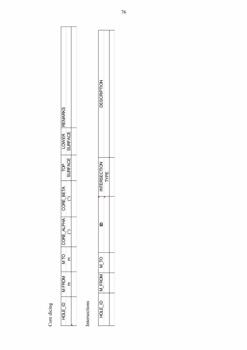
Cor
e di
cing
Inte
rsec
tion
s
HO
LE_I
DM
FR
OM
M T
OC
OR
E_A
LPH
AC
OR
E_B
ETA
TOP
LOW
ER
RE
MA
RK
Sm
m(°
)(°
)S
UR
FA
CE
SU
RF
AC
E
HO
LE_I
DM
_FR
OM
M_T
OID
INTE
RS
EC
TIO
ND
ES
CR
IPTI
ON
TYP
E
76

AP
PE
ND
IX 2
. An
exam
ple
of s
yste
mat
ical
tunn
el m
appi
ng s
heet
. Inv
esti
gati
on n
iche
3 c
hain
age
47.6
-50.
8 m
GE
OL
OG
ICA
L M
AP
PIN
G O
F O
NK
AL
Oda
tein
itial
s
Site
PL
from
Tun
nel d
irect
ion
Map
pin
g da
te/t
ime
Pag
eC
he
ck
ed
Tun
nel I
DP
L to
Tun
nel d
ipG
eolo
gist
Pic
ture
file
Ap
pro
ve
d
Rou
nd I
D
Not
es: R
QD
JnJw
1
JrJa
CA
LC
UL
AT
ED
VA
LU
ES
FO
R Q
-CL
AS
SIF
ICA
TIO
N1
st q
uar
ter
1.5
01.
00
NO
T F
OR
AL
L F
RA
CT
UR
ES
Av
era
ge
1.5
01.
00
3rd
qu
arte
r1
.50
1.00
Med
ian
2.5
01.
00
DIR
DIP
Jr
JaF
.A.
FR
AC
TU
RE
SE
T O
RIE
NT
AT
ION
SE
T1
58
81.
51
56
ES
TIM
AT
ED
US
ING
DIP
SS
ET
2
SE
T3
SE
T4
Len
gth
Co
un
t o
f f r
Ex
trem
ely
Q' q
ual
ity
Q q
ual
ity
SR
F50
150.
00
150.
003
.00
3.0
0
Q'
Q
Fai
r
1.02
7
150.
003
.00
250.
005
.00
0.0
W.A
.
ON
K-T
KU
-362
0-46
.7
0 1:50
46.
7
50.
8
26.1
0.20
09O
NK
AL
O
ON
K-T
KU
-362
0
100
1
Con
sist
s of
DG
N,
neos
ome
cont
ent5
0%.
Larg
e P
GR
incl
usio
ns in
bot
h w
alls
and
on
the
flo
or.
Sev
eral
sub
ever
tica
l fra
ctur
es in
the
roo
f, o
ther
wis
e in
tact
roc
k.
NJK
, R
MA
A
NJK
5.1.
2010
5.1.
2010
ISA
A
Sav
e d
ata
77
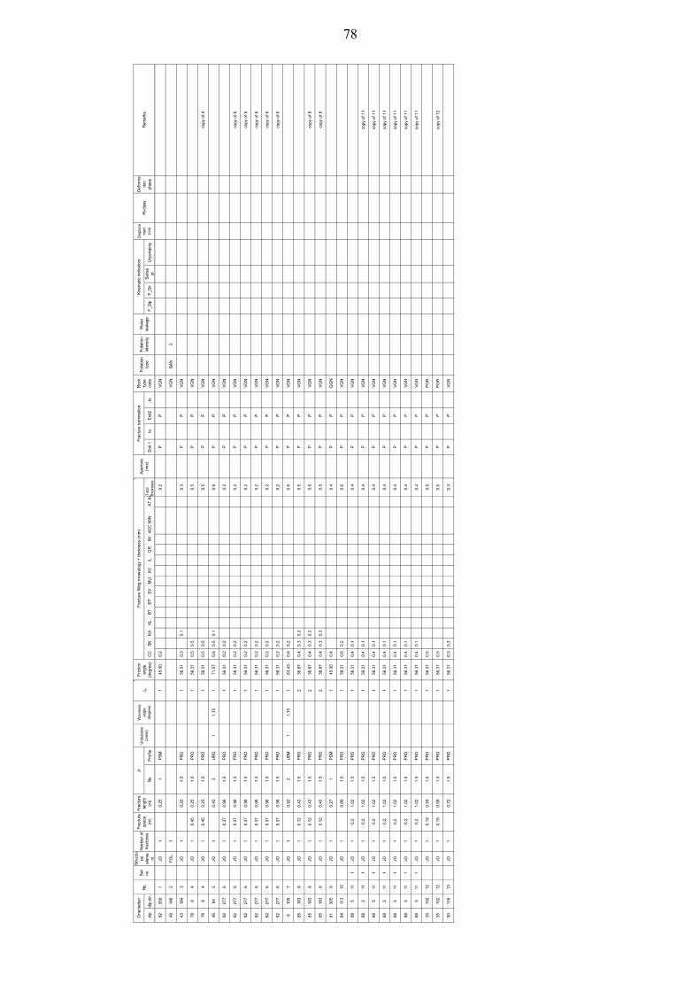
dip
dip
dir.
No.
Pro
file
CC
SK
KA
KL
BT
EP
SV
MU
KV
ILG
RIM
AC
C M
INA
T A
cTot
al
thic
knes
sE
nd 1
toE
nd2
toF
_Dip
F_D
irS
ense
of
U
ncer
tain
ty
8235
91
JO1
0.25
1P
SM
145
.00
0.2
0.2
PP
VG
N
4914
82
FO
L1
VG
NB
AN
2
4318
43
JO1
0.25
1.5
PR
O1
56.3
10.
30.
10.
3P
PV
GN
788
4JO
10.
450.
251.
5P
RO
156
.31
0.5
0.5
0.5
PP
VG
N
788
4JO
10.
450.
251.
5P
RO
156
.31
0.5
0.5
0.5
PP
VG
Nco
py o
f 4
4684
5JO
10.
453
UR
O1
1.15
171
.57
0.6
0.5
0.1
0.6
PP
VG
N
8227
76
JO1
0.37
0.98
1.5
PR
O1
56.3
10.
20.
20.
2P
PV
GN
8227
76
JO1
0.37
0.98
1.5
PR
O1
56.3
10.
20.
20.
2P
PV
GN
copy
of
6
8227
76
JO1
0.37
0.98
1.5
PR
O1
56.3
10.
20.
20.
2P
PV
GN
copy
of
6
8227
76
JO1
0.37
0.98
1.5
PR
O1
56.3
10.
20.
20.
2P
PV
GN
copy
of
6
8227
76
JO1
0.37
0.98
1.5
PR
O1
56.3
10.
20.
20.
2P
PV
GN
copy
of
6
8227
76
JO1
0.37
0.98
1.5
PR
O1
56.3
10.
20.
20.
2P
PV
GN
copy
of
6
610
57
JO1
0.92
2U
SM
11.
151
63.4
30.
60.
20.
6P
PV
GN
8518
38
JO1
0.12
0.43
1.5
PR
O2
36.8
70.
40.
30.
30.
5P
PV
GN
8518
38
JO1
0.12
0.43
1.5
PR
O2
36.8
70.
40.
30.
30.
5P
PV
GN
copy
of
8
8518
38
JO1
0.12
0.43
1.5
PR
O2
36.8
70.
40.
30.
30.
5P
PV
GN
copy
of
8
8130
59
JO1
0.27
1P
SM
145
.00
0.4
0.4
PP
QG
N
8411
310
JO1
0.89
1.5
PR
O1
56.3
10.
60.
20.
6P
PV
GN
885
111
JO1
0.2
1.02
1.5
PR
O1
56.3
10.
40.
10.
4P
PV
GN
885
111
JO1
0.2
1.02
1.5
PR
O1
56.3
10.
40.
10.
4P
PV
GN
copy
of
11
885
111
JO1
0.2
1.02
1.5
PR
O1
56.3
10.
40.
10.
4P
PV
GN
copy
of
11
885
111
JO1
0.2
1.02
1.5
PR
O1
56.3
10.
40.
10.
4P
PV
GN
copy
of
11
885
111
JO1
0.2
1.02
1.5
PR
O1
56.3
10.
40.
10.
4P
PV
GN
copy
of
11
885
111
JO1
0.2
1.02
1.5
PR
O1
56.3
10.
40.
10.
4P
PV
GN
copy
of
11
885
111
JO1
0.2
1.02
1.5
PR
O1
56.3
10.
40.
10.
4P
PV
GN
copy
of
11
3515
212
JO1
0.19
0.59
1.5
PR
O1
56.3
10.
50.
5P
PP
GR
3515
212
JO1
0.19
0.59
1.5
PR
O1
56.3
10.
50.
5P
PP
GR
copy
of
12
9011
613
JO1
0.72
1.5
PR
O1
56.3
10.
30.
30.
3P
PV
GN
Fric
tion
angl
e (d
egre
e)
Wav
ines
s an
gle
(deg
ree)
Ape
rtur
e (m
m)
J a
JrF
ract
ure
leng
ht
(m)
Orie
ntat
ion
Num
ber
of
frac
ture
sS
et
no.
Fra
ctur
e sp
ace
(m
)N
o.
Str
uctu
ral
elem
ent
Def
orm
atio
n ph
ase
Dis
plac
em
ent
(cm
) R
emar
ksF
olia
tion
inte
nsity
Wat
er
leak
age
Ri-c
lass
Kin
emat
ic in
dica
tors
Und
ulat
ion
(cm
/m)
Fra
ctur
e fil
ling
min
eral
ogy
+ t
hick
ness
(m
m)
Fra
ctur
e te
rmin
atio
nR
ock
type
co
de
Fol
iatio
n ty
pe
78

APPENDIX 3. Q-class (Barton 1974).
1. ROCK QUALITY DESIGNATION RQD
A. Very poor 0 ‐ 25 1. 0‐25
B. Poor 25‐50
C. Fair 50‐75
D. Good 75‐90
E. Excellent 90‐100
2. JOINT SET NUMBER Jn
A. Massive, no or few joints 0.5‐1.0
B. One joint set 2
C. One joint set plus random joints 3
D. Two joint sets 4
E. Two joint sets plus random joints 6
F. Three joint sets 9
G. Three joint sets plus random joints 12
H. Four or more joint sets, random, heavily jointed, "sugar cube" etc. 15
J. Crushed rock, earthlike 20 20
3. JOINT ROUGHNESS NUMBER Jr
a. Rock wall contact and b. Rock wall contact before 10 cm shear
A. Discontinuous joints 4
B. Rough and irregular, undulating 3
C. Smooth undulating 2
D. Slickensided undulating 1.5
E. Rough or irregular, planar 1.5
F. Smooth, planar 1
G. Slickensided, planar 0.5
c. No rock wall contact when sheared
H. Zones containing clay minerals enough to 1
prevent rock wall contact
J. Sandy, gravely or crushed zone thick enough to 1
prevent rock wall contact
79

4. JOINT ALTERATION NUMBER ɸr approx. Ja
a. Rock wall contact (no mineral fillings, only coatings)
A. Tightly healed, hard, non‐softening, impermeable 0.75
filling are intended as an approximate guide
B. Unaltered joint walls, surface staining only 25‐35° 1
C. Slightly altered joint walls, non‐softening mineral 25‐30° 2
coatings, sandy particles, clay‐free disintegrated rock, etc.
D. Silty‐, or sandy‐clay coatings, small clay fraction (non‐softening) 20‐25° 3
E. Softening or low‐friction clay mineral coatings, 8‐16° 4
i.e. kaolinite, mica. Also chlorite, talc, gypsum and graphite etc.
and small quantities of swelling clays.
b. Rock wall contact before 10 cm shear (thin mineral filling)
F. Sandy particles, clay‐free, disintegrating rock etc. 25‐30° 4
G. Strongly over‐consolidated, non‐softening clay mineral fillings 16‐24° 6
(continuous < 5 mm thick)
H. Medium or low over‐consolidation, softening clay mineral fillings 12‐16° 8
(continuous < 5 mm thick)
J. Swelling clay fillings, i.e. montmorillonite (continuous < 5 mm thick) 6‐12° 8.0‐12.0
Values of Ja depend on percent of swelling clay‐size particles
and access to water.
c. No rock wall contact when sheared (thick mineral filling)
K, L, M. Zones or bands of disintegrated or crushed rock and clay 6‐24° 6, 8, or 8‐12
(see G, H and J for clay conditions
N. Zones or bands of silty‐ or sandy‐clay, small clay fraction 5
(non‐softening)
O. Thick continuous zones or bands of clay 6‐24° 10, 13 or 13‐20
(see G.H and J for clay conditions)
5. JOINT WATER REDUCTION approx. water pressure
(kgf/cm2)Jw
A. Dry excavation or minor inflow, i.e., <5l/min locally <1 1
B. Medium inflow or pressure, occasional outwash of joint fillings 1.2‐5.0 0.66
C. Large inflow or high pressure in competent rock with unfilled joints 2.5‐10.0 0.5
D. Large inflow or high pressure, considerable outwash of fillings 2.5‐10.0 0.33
E. Exceptionally high inflow or pressure at blasting, decaying with time >10 0.2‐0.1
F. Exceptionally high inflow or water pressure continuing witout >10 0.1‐0.05
noticeable decay
80

6. STRESS REDUCTION FACTOR SRF
a. Weakness zones intersecting excavation, which may
cause loosening of rock mass when tunnel is excavated
A. Multiple occurrences of weakness zones containing clay or 10
chemically disintegrated rock, very loose surrounding rock any
depth)
B. Single weakness zones containing clay, or chemically distegrated rock 5
(excavation depth < 50 m)
C. Single weakness zones containing clay, or chemically distegrated rock 2.5
(excavation depth > 50 m)
D. Multiple shear zones in competent rock (clay free), loose 7.5
surrounding rock (any depth)
E. Single shear zone in competent rock (clay free). (depth of excavation 5
< 50 m)
F. Single shear zone in competent rock (clay free). (depth of excavation 2.5
> 50 m)
G. Loose open joints, heavily jointed or "sugar cube", etc. (any depth) 5
b. Competent rock, rock stress problems σc‐σ1 σt‐σ1 SRF
H. Low stress near surface >200 <0.01 2.5
J. Medium stress, favourable stress condition 200‐10 0.01‐0.3 1
K. High stress, very tight structure, Usually favourable to stability, may be 10.0‐5.0 0.3‐0.4 0.5‐2
unfavourable for wall stability
L. Moderate slabbing after >1 hour in massive rock 5.0‐3.0 0.5‐0.65 5.0‐50.0
M. Slabbing and rock bursts after a few minutes in massive rock 3.0‐2.0 0.65‐1 50‐200
N. Heavy rock bursts (strain‐bursts) and immediate dynamic deformations <2 >1 200‐400
in massive rock
c. Squeezing rock: plastic flow in incompetent rock under the influence of σt‐σ1 SRF
high rock pressure 5.0‐10.0
O. Mild squeezing rock pressure 1.0‐5.0 10.0‐20
P. Heavy squeezing rock pressure >5 10.0‐20.0
d. Swelling rock: plastic flow of incompetent rock under the influence of SRF
high rock pressure
R. Mild swelling rock pressure 5.0‐10.0
S. Heavy swelling rock pressure 10.0‐15.0
81

APPENDIX 4. An example of the drill hole geophysics of the drill hole ONK-PP413 presented in Wellcad sheet
82
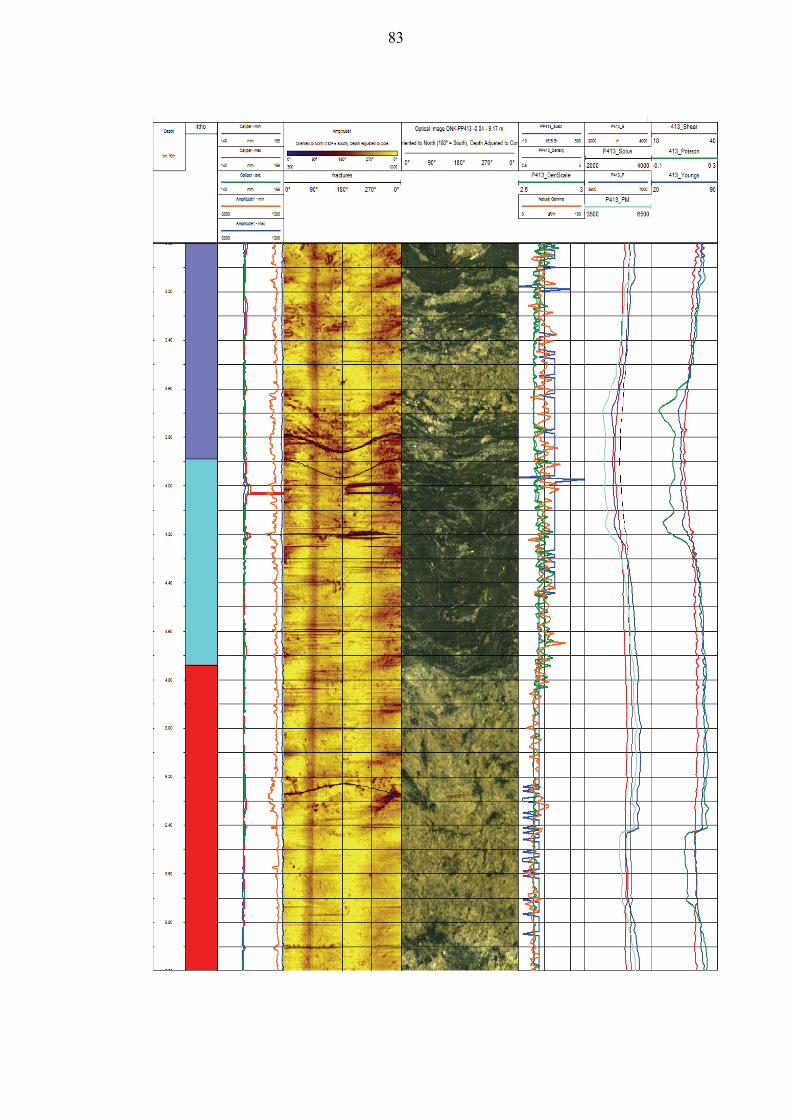
83

84

AP
PE
ND
IX 5
. An
exam
ple
of m
ise-
á-la
-mas
se m
easu
rem
ents
. Ano
mal
ies
in th
e cu
rren
t of
bolt
2 h
as m
arke
d w
ith
blac
k bo
xes.
85
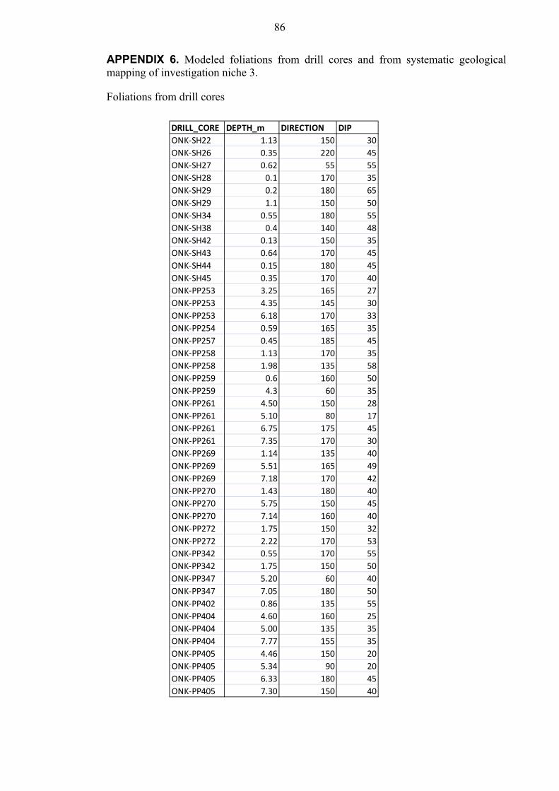
APPENDIX 6. Modeled foliations from drill cores and from systematic geological mapping of investigation niche 3.
Foliations from drill cores
DRILL_CORE DEPTH_m DIRECTION DIP
ONK‐SH22 1.13 150 30
ONK‐SH26 0.35 220 45
ONK‐SH27 0.62 55 55
ONK‐SH28 0.1 170 35
ONK‐SH29 0.2 180 65
ONK‐SH29 1.1 150 50
ONK‐SH34 0.55 180 55
ONK‐SH38 0.4 140 48
ONK‐SH42 0.13 150 35
ONK‐SH43 0.64 170 45
ONK‐SH44 0.15 180 45
ONK‐SH45 0.35 170 40
ONK‐PP253 3.25 165 27
ONK‐PP253 4.35 145 30
ONK‐PP253 6.18 170 33
ONK‐PP254 0.59 165 35
ONK‐PP257 0.45 185 45
ONK‐PP258 1.13 170 35
ONK‐PP258 1.98 135 58
ONK‐PP259 0.6 160 50
ONK‐PP259 4.3 60 35
ONK‐PP261 4.50 150 28
ONK‐PP261 5.10 80 17
ONK‐PP261 6.75 175 45
ONK‐PP261 7.35 170 30
ONK‐PP269 1.14 135 40
ONK‐PP269 5.51 165 49
ONK‐PP269 7.18 170 42
ONK‐PP270 1.43 180 40
ONK‐PP270 5.75 150 45
ONK‐PP270 7.14 160 40
ONK‐PP272 1.75 150 32
ONK‐PP272 2.22 170 53
ONK‐PP342 0.55 170 55
ONK‐PP342 1.75 150 50
ONK‐PP347 5.20 60 40
ONK‐PP347 7.05 180 50
ONK‐PP402 0.86 135 55
ONK‐PP404 4.60 160 25
ONK‐PP404 5.00 135 35
ONK‐PP404 7.77 155 35
ONK‐PP405 4.46 150 20
ONK‐PP405 5.34 90 20
ONK‐PP405 6.33 180 45
ONK‐PP405 7.30 150 40
86

Foliations from systematic geological mapping
MEASUREMENT_NUMBER DIRECTION DIP
1 180 73
2 186 71
3 168 49
4 168 38
5 167 52
6 167 38
7 174 45
8 195 65
9 152 55
10 167 52
11 191 59
12 154 52
13 150 39
14 144 38
15 145 49
16 185 48
17 147 42
18 181 47
19 181 58
20 178 62
21 180 70
22 175 51
23 105 52
24 128 46
25 180 52
26 146 55
27 167 51
28 175 60
29 159 52
30 175 45
31 151 47
32 165 45
33 151 48
34 146 38
35 176 65
36 177 63
37 168 53
38 151 58
39 181 73
40 172 49
41 157 52
42 154 23
43 132 51
44 80 30
87

APPENDIX 7. Orientations of modeled fractures from drill cores and from systematic geological mappings of investigation niche 3.
Fractures from drill cores
DRILL_CORE DEPTH_m DIRECTION DIP FRACTURE_TYPE REMARKS
ONK‐SH28 0.97 190 35 slickenside
ONK‐SH35 0.46 270 19 filled
ONK‐SH36 0.47 180 45 filled
ONK‐PP200 13.48 177 75 filled
ONK‐PP200 17.13 179 89 filled
ONK‐PP200 26.85 140 83 filled
ONK‐PP200 40.75 158 23 filled
ONK‐PP254 1.06 170 34 filled
ONK‐PP256 1.9 155 35 filled
ONK‐PP258 2.89 125 10 filled
ONK‐PP259 4.89 160 28 filled
ONK‐PP261 7.49 160 31 slickenside
ONK‐PP261 5.2 200 55 filled
ONK‐PP268 5.68 164 32 slickenside
ONK‐PP268 6.23 164 40 slickenside
ONK‐PP268 6.28 164 36 slickenside
ONK‐PP268 6.45 164 40 slickenside
ONK‐PP269 6.41 170 44 slickenside
ONK‐PP269 6.42 170 41 slickenside
ONK‐PP270 4.36 160 56 filled
ONK‐PP270 6.38 160 40 filled
ONK‐PP270 6.44 160 40 filled
ONK‐PP271 6.4 164 12 slickenside
ONK‐PP271 6.46 164 20 slickenside
ONK‐PP340 6.28 170 40 slickenside dir and dip unsure. Value evaluated from the foliation direction
ONK‐PP340 6.49 165 45 slickenside dir and dip unsure. Value evaluated from the foliation direction
ONK‐PP340 6.61 160 40 slickenside dir and dip unsure. Value evaluated from the foliation direction
ONK‐PP340 7.14 165 40 slickenside dir and dip unsure. Value evaluated from the foliation direction
ONK‐PP341 7.28 164 45 slickenside dir and dip unsure. Value evaluated from the foliation direction
ONK‐PP342 0.69 165 35 filled
ONK‐PP342 0.71 135 35 filled
ONK‐PP342 1.25 160 50 filled
ONK‐PP342 1.29 160 50 filled
ONK‐PP346 6.73 170 40 slickenside dir and dip unsure. Value evaluated from the foliation direction
ONK‐PP346 7.25 165 40 slickenside dir and dip unsure. Value evaluated from the foliation direction
ONK‐PP346 7.34 150 50 slickenside dir and dip unsure. Value evaluated from the foliation direction
ONK‐PP346 7.93 160 30 slickenside dir and dip unsure. Value evaluated from the foliation direction
ONK‐PP346 7.73 164 43 grainfilled dir and dip unsure. Value evaluated from the foliation direction
ONK‐PP347 4.12 190 25 slickenside
ONK‐PP347 6.94 285 70 filled
ONK‐PP347 7.25 180 50 slickenside
ONK‐PP347 7.34 160 50 filled
ONK‐PP347 7.39 150 50 grainfilled
ONK‐PP398 2.87 168 15 slickenside
ONK‐PP398 4.5 139 28 filled
ONK‐PP398 7.93 147 40 slickenside
ONK‐PP398 8.09 126 41 slickenside
ONK‐PP399 0.68 138 46 filled
ONK‐PP400 1.26 167 42 slickenside
ONK‐PP400 1.84 112 30 filled
ONK‐PP400 1.93 91 30 filled
ONK‐PP401 1.42 133 40 slickenside
ONK‐PP401 1.54 94 28 filled
ONK‐PP401 1.58 114 40 slickenside
ONK‐PP401 6.73 127 36 filled
ONK‐PP401 9.94 168 49 filled
ONK‐PP401 10.07 177 5 filled
ONK‐PP401 10.11 122 39 slickenside
ONK‐PP401 10.54 145 24 filled
88

ONK‐PP402 0.99 131 48 slickenside
ONK‐PP402 1.11 338 35 slickenside
ONK‐PP402 1.18 125 41 filled
ONK‐PP402 5.39 78 11 filled
ONK‐PP402 5.57 152 41 filled
ONK‐PP402 9.86 168 24 filled
ONK‐PP402 9.87 149 31 slickenside
ONK‐PP402 9.89 157 41 slickenside
ONK‐PP402 9.97 157 30 filled
ONK‐PP402 10.32 187 21 filled
ONK‐PP402 10.39 128 22 filled
ONK‐PP403 9.1 121 94 filled
ONK‐PP404 7.72 190 53 filled
ONK‐PP404 7.76 160 52 slickenside
ONK‐PP404 7.97 125 50 slickenside
ONK‐PP404 8 124 35 slickenside
ONK‐PP404 8.09 140 15 filled
ONK‐PP404 8.15 195 40 filled
ONK‐PP404 8.16 185 40 slickenside
ONK‐PP404 8.18 110 5 slickenside
ONK‐PP404 8.21 150 20 filled
ONK‐PP405 4.19 3 12 filled
ONK‐PP405 5.85 200 35 slickenside
ONK‐PP405 7.53 41 15 slickenside
ONK‐PP405 7.6 162 57 slickenside
ONK‐PP405 7.63 146 46 slickenside
ONK‐PP405 7.67 147 27 slickenside
ONK‐PP410 3.79 169 30 slickenside
ONK‐PP410 5.24 33 19 clayfilled
ONK‐PP410 5.61 135 45 filled
ONK‐PP410 7.53 170 48 filled
ONK‐PP410 7.62 163 45 filled
ONK‐PP411 6.52 127 34 slickenside
ONK‐PP411 6.55 34 42 slickenside
ONK‐PP411 6.98 174 52 filled
ONK‐PP412 2.65 164 42 slickenside
ONK‐PP412 2.98 20 24 slickenside
ONK‐PP412 3.22 126 38 filled
ONK‐PP413 3.82 173 44 filled
ONK‐PP413 3.92 177 48 slickenside
89
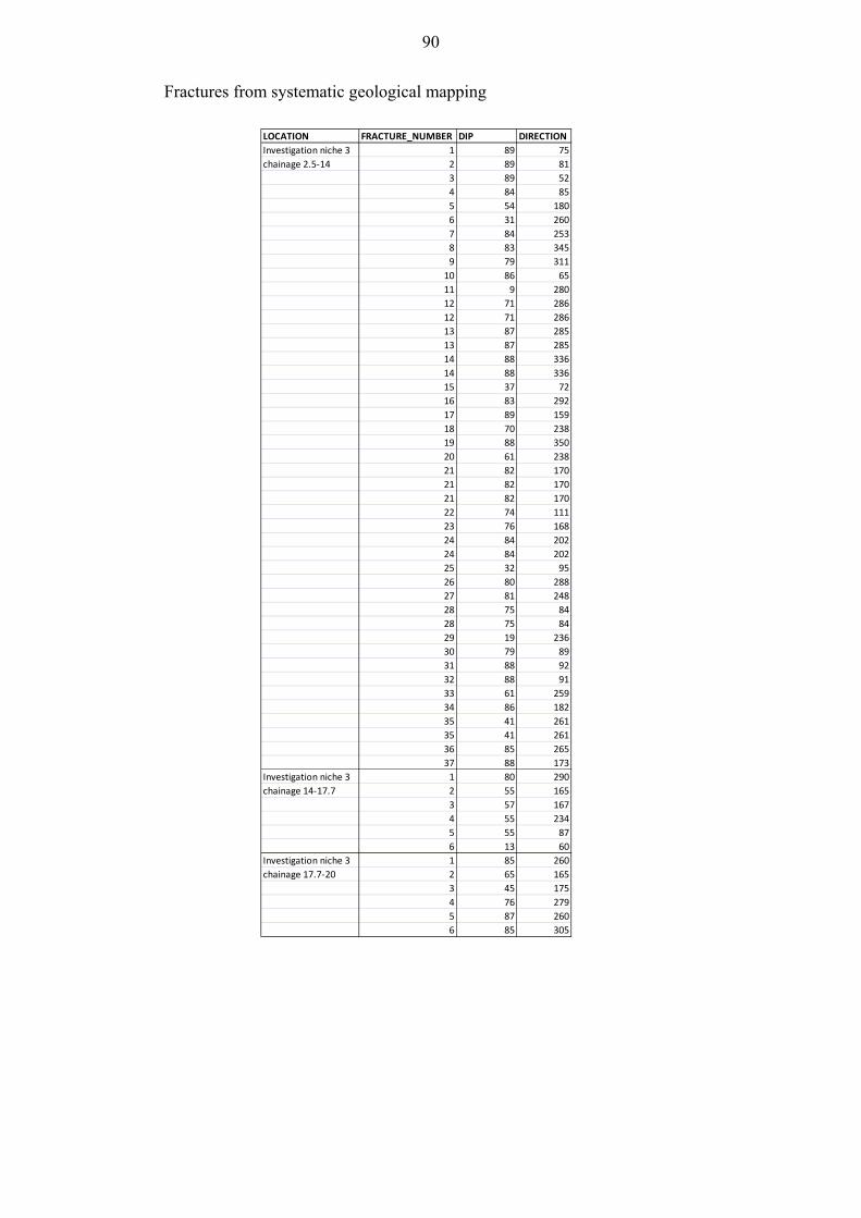
Fractures from systematic geological mapping
LOCATION FRACTURE_NUMBER DIP DIRECTION
Investigation niche 3 1 89 75
chainage 2.5‐14 2 89 81
3 89 52
4 84 85
5 54 180
6 31 260
7 84 253
8 83 345
9 79 311
10 86 65
11 9 280
12 71 286
12 71 286
13 87 285
13 87 285
14 88 336
14 88 336
15 37 72
16 83 292
17 89 159
18 70 238
19 88 350
20 61 238
21 82 170
21 82 170
21 82 170
22 74 111
23 76 168
24 84 202
24 84 202
25 32 95
26 80 288
27 81 248
28 75 84
28 75 84
29 19 236
30 79 89
31 88 92
32 88 91
33 61 259
34 86 182
35 41 261
35 41 261
36 85 265
37 88 173
Investigation niche 3 1 80 290
chainage 14‐17.7 2 55 165
3 57 167
4 55 234
5 55 87
6 13 60
Investigation niche 3 1 85 260
chainage 17.7‐20 2 65 165
3 45 175
4 76 279
5 87 260
6 85 305
90

Investigation niche 3 1 51 89
chainage 20‐30 2 86 241
3 71 104
4 49 172
5 88 268
6 80 273
7 18 288
8 82 252
9 83 84
10 33 22
11 68 71
12 45 77
13 79 282
14 76 70
15 89 251
16 72 88
17 36 169
18 57 38
Investigation niche 3 1 85 342
chainage 30‐40 2 78 316
3 82 341
4 46 349
5 76 81
6 76 81
7 71 339
8 80 86
9 49 22
10 49 22
11 49 22
12 85 165
13 42 357
14 45 6
15 50 59
16 82 36
17 85 67
18 71 248
Investigation niche 3 1 51 132
chainage 40‐50 2 25 263
3 84 335
4 79 341
4 79 341
4 79 341
5 81 281
6 88 81
7 78 144
7 78 144
8 18 246
9 29 139
10 75 354
10 75 354
10 75 354
10 75 354
10 75 354
10 75 354
10 75 354
11 82 79
12 73 264
13 78 254
14 81 275
15 85 146
15 85 146
16 61 39
17 80 260
17 80 260
18 73 256
19 81 256
20 32 282
21 90 76
21 90 76
22 84 55
23 85 251
24 76 112
25 88 159
91

Investigation niche 3 1 75 345
chainage 50‐60 2 85 215
3 84 227
3 84 227
3 84 227
3 84 227
3 84 227
4 88 230
5 80 205
6 89 236
7 85 232
8 88 208
9 85 218
10 85 180
11 70 115
12 31 160
12 31 160
12 31 160
13 35 148
14 40 215
15 85 215
16 30 80
17 80 335
17 80 335
17 80 335
18 82 334
18 82 334
19 80 340
20 87 165
20 87 165
21 85 332
22 80 32
23 80 340
24 30 35
25 88 33
26 71 32
27 76 295
28 84 70
29 25 285
30 85 5
31 83 140
32 89 168
33 80 135
Investigation niche 3 1 48 205
chainage 60‐70 2 70 240
3 82 265
3 82 265
3 82 265
3 82 265
4 89 270
4 89 270
4 89 270
5 78 325
6 85 42
7 85 335
8 35 100
9 15 125
10 35 88
11 18 215
12 80 150
13 45 145
14 80 245
15 80 255
92

ONK‐TKU_3620_floor 1 57 247
2 85 270
3 82 271
4 48 145
5 76 119
6 36 151
7 49 285
8 67 280
9 51 81
10 74 346
11 80 276
12 79 150
13 84 169
14 88 281
15 80 350
16 77 266
17 68 285
18 85 156
19 88 319
20 68 145
21 81 280
22 78 283
23 76 280
24 29 176
25 69 269
26 84 276
27 76 98
28 37 346
29 71 282
30 82 99
31 78 271
32 56 157
33 43 168
93

AP
PE
ND
IX 8
. Phy
sica
l pro
pert
ies
of r
ock
by E
ero
Hei
kkin
en (
Pöy
ry F
inla
nd O
y). M
odel
ed z
ones
are
mar
ked
in th
e ta
ble.
Drillhole
Sec_Up
Sec_Down
Description
Den
sity
Suscep
tibility
Natural G
amma
Resistivity
Seismic velocities
Youngs m
odulus
Shear modulus
Poisson's ratio
ONK‐PP398
01Interval affected by concrete slab and ED
ZPG
R average
Elevated
Average
Decreased
Decreased
Lowered
Lowered
Spurious
ONK‐PP398
12.7Average PGR
PGR average
Diamagnetic‐Paramagnetic
Low
Average PGR
Average or slightly lowered
PGR, P wave stAverage
Average
Scattered, low
ONK‐PP398
2.7
3.4PG
R with VGN intersections
VGN sho
ws elevated
Sligtly ferrimag
Sligthly elevated in VGN
Average, slight low in VGN
Average, slightly elevated in VGN
Average, slightly elevated in
VGN
Average, slightly elevated
in VGN
Average
ONK‐PP398
3.4
4.2Average PGR
PGR average
Paramagnetic
Average
Average PGR
Average PGR
Average
Average
Average
ONK‐PP398
4.2
4.73
Anomalous VGN
Clearly elevated
Elevated
(ferrim
ag)
Average
Conductive
Clearly lowered
Lowered
Lowered
Average
ONK‐PP398
4.73
7.2VGN, high resistivity variant
Average VGN
Low (diamagnetic?)
Average
High
Average
Slightly elevated
Slightly elevated
Average
ONK‐PP398
7.2
8.16
VGN
Average VGN
Average VGN
N/A
N/A
Lowered
Lowered
Lowered
Average
ONK‐PP399
01.1Interval affected by concrete slab and ED
ZAverage VGN
Elevated
Average
Lowered
Lowered
Lowered
Lowered
High/Spurious
ONK‐PP399
1.1
1.55
Average VGN
Average VGN
Average VGN
Average
Lowered
Lowered
Lowered
Lowered
Elevated
ONK‐PP399
1.55
3.4Average PGR
Average PGR
Average PGR
Low, elevated at 2.4m
Average PGR. Lowered
at 2.42m
Average PGR. Lowered
at 2.42m
Average
Average. Lowered
at 2.42
Average
ONK‐PP399
3.4
4.68
PGR with VGN intersections
Average, VGN elev.
Average, VGN elev.
Low, elevated at 4.4m
Average PGR, elevated at 4.1 ‐ 4.6m
Average PGR
Average
Average
Average
ONK‐PP399
4.68
5.43
Anomalous VGN
Clearly elevated
Elevated
(ferrim
ag)
Average
Conductive
Lowered
Lowered
Lowered
Average
ONK‐PP399
5.43
8.18
VGN, high resistivity variant
Average VGN
Low (diamagnetic?)
Average
High
Average
Slightly elevated
Slightly elevated
Average
ONK‐PP400
01.15
Interval affected by concrete slab and ED
ZAverage DGN
Elevated
Elevated
Lowered
Lowered
Lowered
Lowered
Lowered
ONK‐PP400
1.15
2.5DGN and
fractures
Average DGN
Elevated
(ferrimag)
Slightly elevated
Conductive
Lowered, P spurious
Lowered
Lowered
Spurious
ONK‐PP400
2.5
5.4PG
RAverage PGR
Low (diamagnetic) at top, deeper paramagnetic
Low
Average PGR, locally high
Average PGR
Average
Average
Average
ONK‐PP400
5.4
5.8Anomalous VGN
Average
VGN
Elevated
(ferrim
ag)
Average
Lowered
Slightly lowered
Slightly lowered
Slightly lowered
Average
ONK‐PP400
5.8
7.35
VGN, high res variant
Average VGN
Average VGN (param
ag)
Average
High
Average (high vgn)
Slightly elevated
Slightly elevated
Average
ONK‐PP400
7.35
7.9PG
R (Leucosome)
Average PGR
Low (param
agnetic)
Average
High
Average
Average
Average
Average
ONK‐PP400
7.9
9.46
VGN
Average VGN
Low (diamagnetic)
Average
Lowered
Lowered
Slightly lowered
Slightly lowered
Average
ONK‐PP400
9.46
9.84
Fracture in VGN
Average VGN
Low
Average
Conductive
Low
Low
Low
Spurious
ONK‐PP400
9.84
13PG
RLow PGR
Low (diamagnetic)
Low
Slightly lowered
(fractures)
Average
Average
Average
Average
ONK‐PP401
01.05
Interval affected by concrete slab and ED
ZLow
Elevated
Average
Low
Low
Low
Low
Spurious
ONK‐PP401
1.05
1.85
PGR, fractures and
melanosome?
Elevated
(_GN)
Ferrimag
Average
Conductive
Clearly lowered
Clearly low
Clearly low
Low
ONK‐PP401
1.85
9.45
PGR, some fracture sets
Average PGR
Average PGR
Low, elev vein at 3.52
Average PGR, fractures 2.87m
, 5.83m
, 6. 6Average, slight low at fractures
Average, low at fracs
Average, low at fracs
Average
ONK‐PP401
9.45
10.65VGN, anomalous
Average
VGN
Average
VGN
Average
Conductive, possibly graphite
Clearly lowered
Clearly low
Clearly low
Lowered
ONK‐PP401
10.65
13.12PG
RAverage PGR
diam
gnetic
Average
Average PGR
Average
Average
Average
Average
ONK‐PP402
01.55
Interval affected by concrete slab and ED
ZAverage
Elevated
Elevated
Conductive
Low
Low
Low
Spurious
ONK‐PP402
1.55
1.71
VGN and
PGR, fractures
Average VGN
Elevated
average
Conductive
Low
Low
Low
Spurious
ONK‐PP402
1.71
9.4PG
RAverage PGR
Average PGR
Average, spikes at3, 4.47, 5.58, 8.4 m.Average, fractures at 4.54
and
5.88 m, lowAverage, lowered
below 7.9 m
Average
Average
Average
ONK‐PP402
9.4
10.56VGN, fractures
Average VGN
Ferrimagnetic
Varying, partly elevated
Conductive
Low
Very low
Very low
Lowered
ONK‐PP402
10.56
13.14PG
RAverage PGR
Diamagnetic
Low
Average
Slightly elevated
Average
Average
Average
ONK‐PP403
01.4Interval affected by concrete slab and ED
ZLow
Average PGR
Average
Low
Low
Low
Low
Spurious
ONK‐PP403
1.4
3.55
PGR, partly desaturated of water
Average PGR
Elevated
PGR (ferrimag?)
Low
Average PGR
Average PGR
Average
Average
Low, desaturation
ONK‐PP403
3.55
6.3PG
R, locally melanosome. Gradational lower cvarying btw PGR & intersections
Elevated
(partly ferrimag)
Average
Clearly lowered
(fractures)
Clearly lowered
(fractures)
Lowered
Lowered
Lowered, spiky
ONK‐PP403
6.3
8.7PG
R, typical
Average PGR
Average PGR
Top part low, then average.
Average or slightly lowered
Average PGR
Average
Average
Average
ONK‐PP403
8.7
9.92
VGN, anomalous
Average
VGN (or slightly elevated
)Av. VGN, p
artly ferrim
agAverage
Conductive
Clearly lowered
Clearly lowered
Clearly lowered
Average
ONK‐PP403
9.92
12.37PG
RAverage PGR
Diamagnetic
Average
Average PGR
Average PGR
Average
Average
Average
ONK‐PP403
12.37
13.19DGN
Average DGN
Average DGN
N/A
N/A
N/A
N/A
N/A
N/A
94
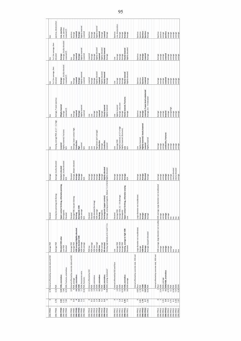
ONK‐PP404
00.78
Interval affected
by concrete slab and EDZ
Average PGR
Elevated
Average
low
low
low
low
low
ONK‐PP404
0.78
4.33
PGR
Average PGR
Varying low paramag and
diamag
Average, locally elevated
Varying, average PGR, at 2.7 ‐ 3.1 high.
Average, P wave spurious
To 2.5m average, then
elevated
To 2.5m average, then
elevated
spurious, desaturation
ONK‐PP404
4.33
5.22
VGN, anomalous
Elevated VGN value
Upper contact ferrim
ag, otherw
ise paramag.
Contacts elevated
Lowered
Slihgtly lowered
Average
Average
Low, spurious
ONK‐PP404
5.22
7.64
Low PGR
Diamagnetic
Average, locally elev ated
Slightly lowered, fractures
Average
Average, locally elevated
Average, locally elevated
Low, spurious
ONK‐PP404
7.64
8.25
VGN, fractures, ano
malous
Elevated
Elevated
N/A
N/A
Lowered
(?)
Lowered
(?)
Lowered (?)
Lowered
(?)
ONK‐PP405
00.9Interval affected
by concrete slab and EDZ
Average PGR
Elevated
Elevated
Low
Low
low
low
spurious
ONK‐PP405
0.9
4PG
R, average
Average PGR
Average PGR, top part diamag
Average, deeper elevated
Average, lower contact high.
Average
Average
Average
Average
ONK‐PP405
44.6VGN, anomalous
VGN average/sligthly elevated
Ferrim
agAverage
Conductive
Lowered
Lowered
Lowered
Lowered
ONK‐PP405
4.6
5.6VGN
Slighly elevated VGN
diamagnetic VGN
Average
High
Average
Average
Average
Average
ONK‐PP405
5.6
7.7VGN, leucosome veins
VGN av erage
VGN average
Average
Lowered
Sligtlhy lowered
Slightly lowered
Slightly lowered
Slightly lowered
ONK‐PP405
7.7
8.16
PGR, fractures
PGR average
N/A
N/A
N/A
Lowered
Lowered
Lowered
Lowered
ONK‐PP410
00.5Interval affected
by EDZ
PGR low
Elevated
Average
Low
Low
Lowered
Lowered
Spurious
ONK‐PP410
0.5
0.8PG
RPGR average
Elevated
Average
Low
Low
Average
Average
Average
ONK‐PP410
0.8
1.9VGN, ano
malous
VGN low
VGN elevated (ferrimag)
Average
Low
Average
Average
Average
Average
ONK‐PP410
1.9
3.4VGN
VGN average
VGN average
Average
High (lo
wer part average)
Average
Slightly elevated
Slightly elevated
Slightly lowered
ONK‐PP410
3.4
4.2VGN, anomalous
VGN low
Ferrim
agAverage
Conductive
Lowered
Lowered
Lowered
Lowered
ONK‐PP410
4.2
5.2PG
RPGR average
Diamagnetic
Average
Average
Average
Slightly elevated
Slightly elevated
Average
ONK‐PP410
5.2
6DGN, anomalous
GN elevated
Ferrim
agnetic (upper contact)
Slightly elevated
Conductive
Clearly lo
were d
Clearly lowered
Clearly lowered
Lowered
ONK‐PP410
69.06
DGN; varying, inclusions?
Varying, high density at 6.3 and
7.5 m
Average, varying paramagnetic. B
elow 7.1 m
ferrimSlightly elevated
Lowered
Slightly lowered
Average
Average
Average
ONK‐PP411
01Interval affected
by EDZ and floor
Low
Elevated
Average
Low
Low
Low
Low
Spurious
ONK‐PP411
11.8PG
RAverage PGR
Average PGR
Average
Average PGR
Slightly lowered
Average
Average
Low, desaturation
ONK‐PP411
1.8
5.3VGN
Average VGN
Average VGN, 3.2 ‐ 4.4 diamagn.
Average
Slightly lowered, at 3.7 m
high
Average, very even
Average
Average
Average
ONK‐PP411
5.3
6.35
PGR
Average PGR
Diamagnetic
Average
Slightly lowered (fractures)
Average
Average
Average
Average
ONK‐PP411
6.35
7.9VGN, anomalous
Varying, average to high VGN
Upper contact ferrim
ag, otherw
ise varying
Average
Low
Clearly lowered
, fractures
Clearly lowered
Clearly lowered
Average
ONK‐PP411
7.9
8.8VGN average
Elevated
Low
N/A
N/A
Average
Slightly elevated
Slightly elevated
Average
ONK‐PP412
00.85
Interval affected
by concrete slab, EDZ and
floor
Large diameter not recalibrated.
Large diameter no
t recalibrated.
Average
Low
Spurious
Spurious
Spurious
Spurious
ONK‐PP412
0.85
1.76
PGR
Average
Average
Average
Slightly lowered
Average
Spurious
Average
Spurious
ONK‐PP412
1.76
2.7VGN
VGN low
Average
Average
Slightly lowered/ clearly lowered
Average
Spurious
Average
Spurious
ONK‐PP412
2.7
3.65
DGN
Average
Varying
Elevated
Lowered
Lowered
, P wave level undetected
Lowered
Lowered
Spurious
ONK‐PP412
3.65
9.35
PGR
Average, top part elevated
Average
Average
Slightly lowered
Average, 6.6 ‐ 7.4 elevated
Average
Average
Average
ONK‐PP413
01
Interval affected
by concrete slab, EDZ and
floor
VGN averag e, large diameter no
t recalibraVGN average, large diameter not recalibrated
Average
Average
Average
Average
Average
Spurious
ONK‐PP413
12.25
VGN
average
average
average
average
average
average
average
spurious
ONK‐PP413
2.25
3.4DGN, average
average
average
average
average
average
average
average
average
ONK‐PP413
3.4
4.2DGN/V
GN, anomalous
average
average
average
conductive, fractures
lowered
Lowered
Lowered
spurious
ONK‐PP413
4.2
4.75
VGN
average
average
average
average
average
average
average
average
ONK‐PP413
4.75
6.1PG
Raverage
low
average
average
average/high
average
average
average
ONK‐PP413
6.1
6.58
PGR
low
low
clearly elevated
average
average
average
average
average
ONK‐PP413
6.58
7.07
DGN
low
low
clearly elevated
average
average
average
average
average
ONK‐PP413
7.07
9.28
DGN
low
low
average
average
average
average
average
average
95

96