geographical economics (second part) urban and regional economics josé luis roig
TRANSCRIPT

GEOGRAPHICAL ECONOMICS (SECOND PART)
URBAN AND REGIONAL ECONOMICS
José Luis Roig

WHAT IS URBAN AND REGIONAL ECONOMICS
Urban and regional economics adds geographical space to the economic analysis of utility-maximizing households and profit-maximizing firms. It lies at the intersection of economics and geography.
Urban and regional economics recognizes that goods are produced at certain locations, traded at some locations and bought by individuals who live at one location and work at another location. Distance between different economic activities implies costs for transporting goods and moving people. Distance also defines communication and social interactions among consumers and workers.

Increasing Urbanization RatesMore than half of the World’s population now lives in cities
Source: UN World Urbanization Prospects, 2009 Revision, esa.un.org/unpd/wup
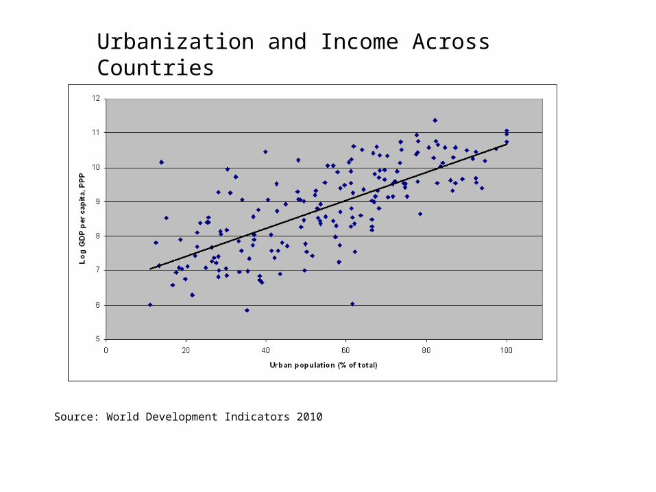
Urbanization and Income Across Countries
Source: World Development Indicators 2010

Urban Concentration in Europe
Population density in 2005 by OECD TL3 region
Source: Kamal-Chaoui and Robert (2009) Competitive Cities and Climate Change
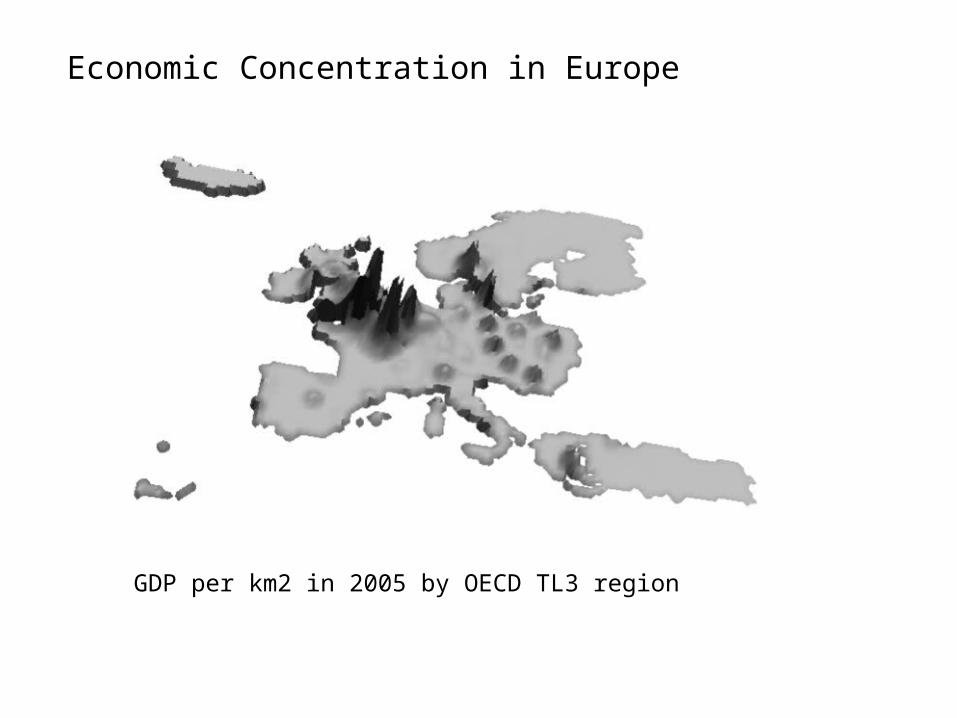
Economic Concentration in Europe
GDP per km2 in 2005 by OECD TL3 region

Productivity increases with employment density
• Elasticity around 5%(U.S.),4.5%(Europe) • Doubling density increases productivity by 5%(4.5%)

Employment in the wine industry (SIC 2084)
Sectoral concentration explained by natural advantages

Employment in the computer software industry (SIC 7371, 7372, 7373, 7375)
No natural advantages

Employment in the Computer Software Industry (SIC 7371, 7372, 7373, 7375) San Francisco

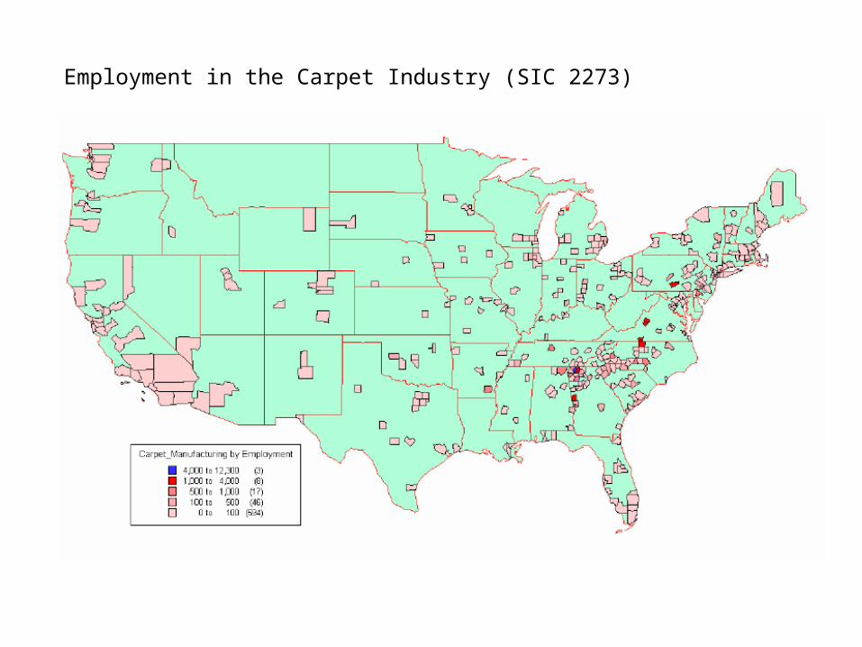
Employment in the Carpet Industry (SIC 2273)
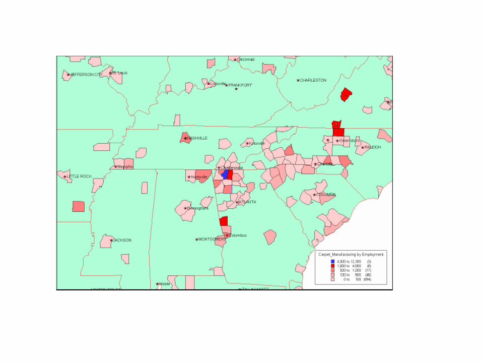

Agglomeration economies
Firms can benefit from the concentration of other firms (A. Marshall):
- Large labour market
- Large market of intermediate input suppliers
- Knowledge spillovers

Strong regional disparities of GDP per capita in EU
- Blue Banana- Nordic Countries- Periphery - Large difference within some countries- Spatial contagion (spatial diffusion of development)

Accessibility and Transport Cost: The Market Potential
4
1
ji
j ijj i
MMP
d
M: Population, GDP, DI,…
GDP level provides a crude measure of economic size of a region. Some insight into the potential of attraction of new activity
Besides its size, one expects the accessibility of a region from others to be another critical determinant of firms’ and workers’ locational decisions
The market potential aims to capture the idea that being close to prosperousregions makes a region more attractive because it offers good access toseveral large markets

Strong core-peripherypattern

•More spatial dispersion. Prosperous states scattered all over the country•Regional disparities are much wider within the European Union than in the United States.
Less strong core-periphery pattern
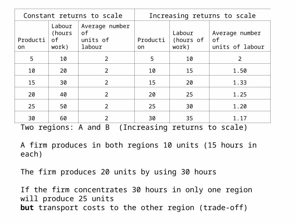
Constant returns to scale Increasing returns to scale
Production
Labour(hours of work)
Average number of units of labour Production
Labour(hours of work)
Average number of units of labour
5 10 2 5 10 2
10 20 2 10 15 1.50
15 30 2 15 20 1.33
20 40 2 20 25 1.25
25 50 2 25 30 1.20
30 60 2 30 35 1.17
Two regions: A and B (Increasing returns to scale)
A firm produces in both regions 10 units (15 hours in each)
The firm produces 20 units by using 30 hours
If the firm concentrates 30 hours in only one region will produce 25 unitsbut transport costs to the other region (trade-off)

Economies of scale describes how average cost decreases as theoutput quantity increases. There are several explanations for thisphenomenon:
1. Indivisible inputs: required to produce one or a thousand units
2. Factor specialization• Learning-by-doing• Continuity• Simpler tasks (specialisation) can be mechanised more easily

Theory of Industrial Location
What leads firms to locate where they do? Can space confer monopoly power? How do compete firms in space? To what extent firms behave rationally in their location
decision?
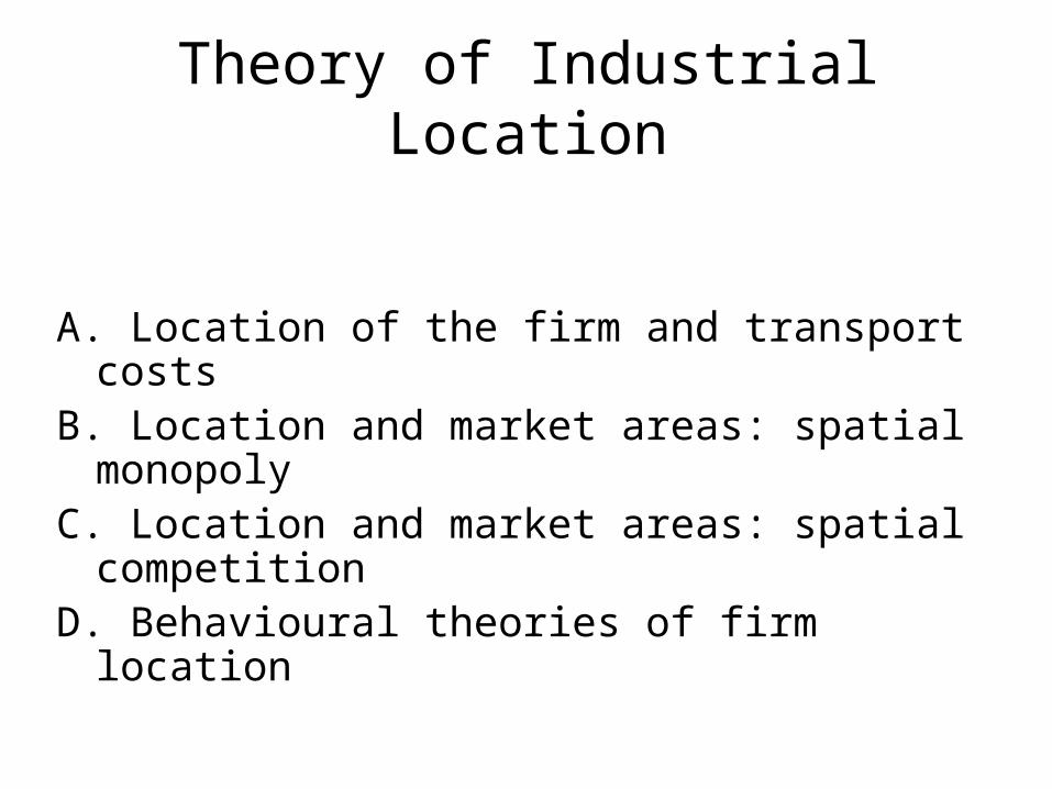
Theory of Industrial Location
A. Location of the firm and transport costsB. Location and market areas: spatial monopoly C. Location and market areas: spatial competitionD. Behavioural theories of firm location

A. Location of the firm and transport costs
• The Weber location-production model (fixed coefficients technology)
• The Moses location-production model (factor substitutability)
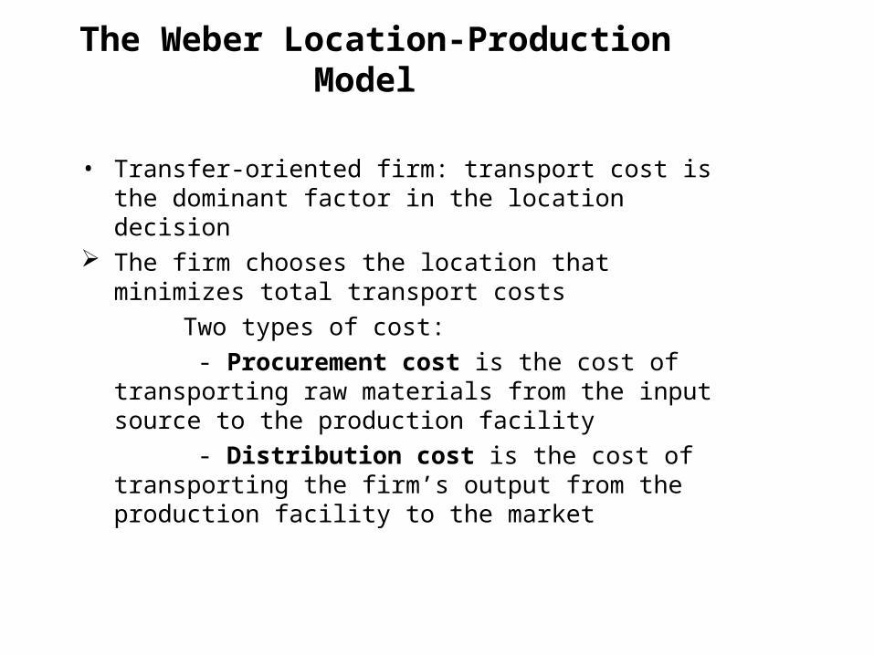
The Weber Location-Production Model
• Transfer-oriented firm: transport cost is the dominant factor in the location decision
The firm chooses the location that minimizes total transport costs
Two types of cost:
- Procurement cost is the cost of transporting raw materials from the input source to the production facility
- Distribution cost is the cost of transporting the firm’s output from the production facility to the market

• Four assumptions:
1. Single transferable output. The firm produces a fixed quantity of a single product, which is transported from the production facility to a market M
2. Single transferable input. The firm may use several inputs, but only one input is transported from an input source, F, to the production facility
3. Fixed-factor proportions. The firm produces its fixed quantity with fixed amounts of each input. No factor substitution
4. Fixed prices. The firm is so small that it does not affect the prices of its input or its output
The only costs that varies across space is transport cost The firm will choose that location that minimizes transport costs
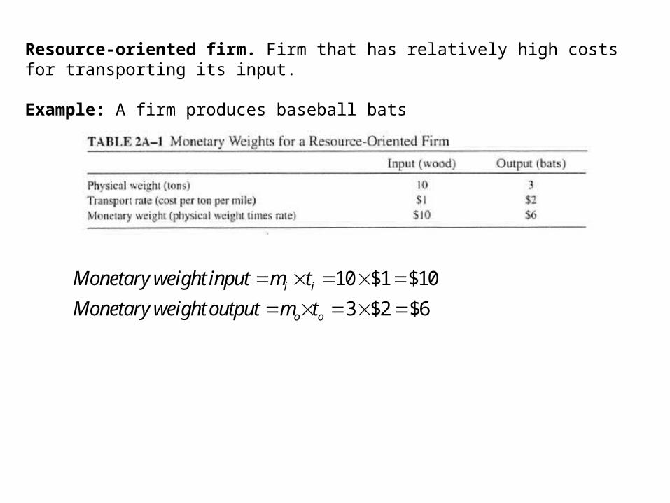
Resource-oriented firm. Firm that has relatively high costs for transporting its input.
Example: A firm produces baseball bats
10 $1 $10
3 $2 $6i i
o o
Monetary weight input m t
Monetary weightoutput m t
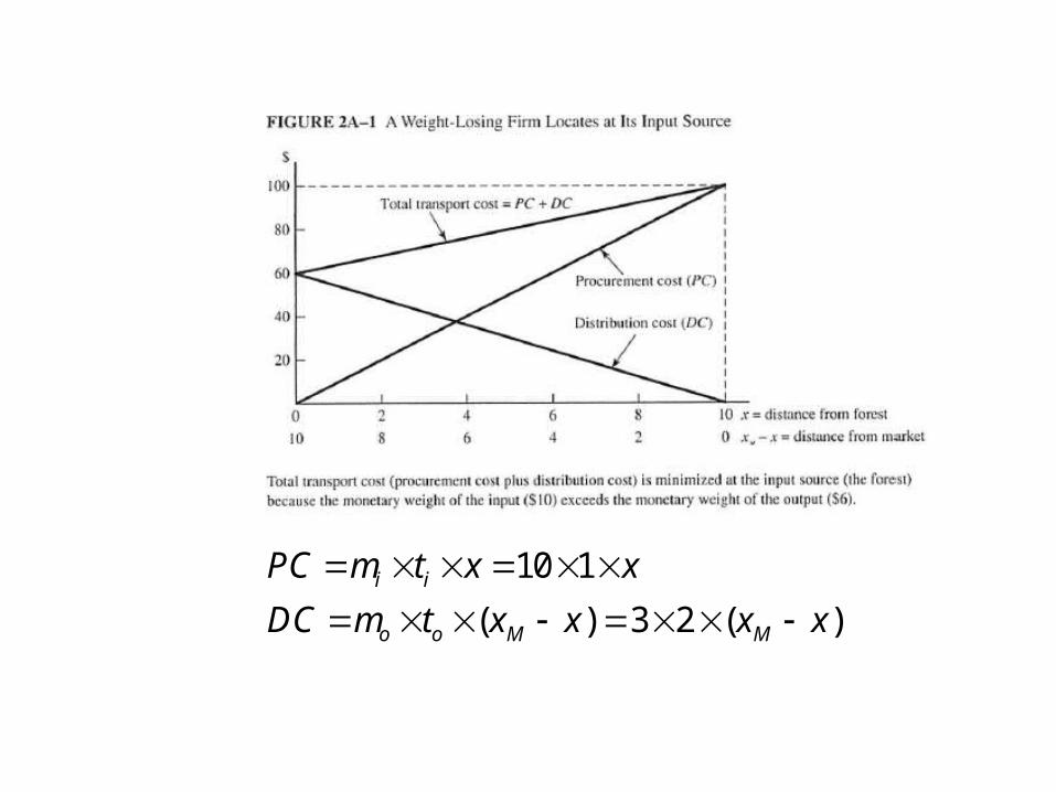
10 1
( ) 3 2 ( )i i
o o M M
PC m t x x
DC m t x x x x

7 tns. of beets needed for 1 tn. of sugar

Market-oriented firm. Firm that has relatively high costs for transporting its output to the market
Example: Bottling firm of beverages
1 $1 $1
4 $1 $4i i
o o
Monetary weight input m t
Monetary weight output m t
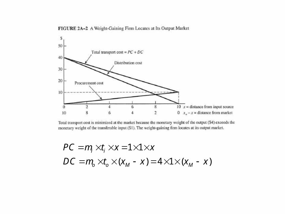
1 1
( ) 4 1 ( )i i
o o M M
PC m t x x
DC m t x x x x

10 tns. of wheat needed for 100 tns. of beer

Two inputs and one market: the Weber location triangle
Example: car manufacturer uses steel and plastic
3 3 1 1 1 1 2 2 2 2 3 3 3( ) ( )p m p t d m p t d m t d m
Profit of the firm:
Given the assumptions of fixed coefficients of inputs and fixed prices:3
1
Min Transport cost = i i ii
m t d
Single establishment – profit maximizer – price taker – perfect competition – 2 inputs single output Critical factors m1 m2 m3; p1 p2 p3; M1 M2 M3; t1 t2 t3; K Maximise profit by minimising total costs
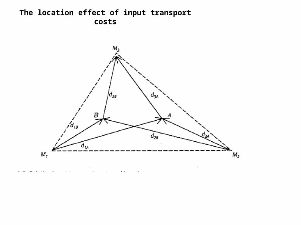
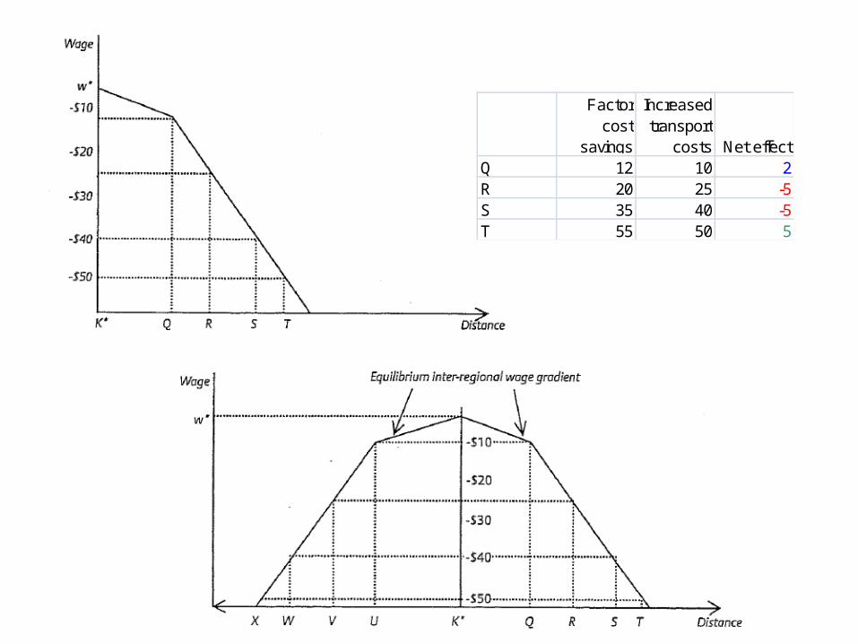
The location effect of input transport costs

The location effect of output transport costs
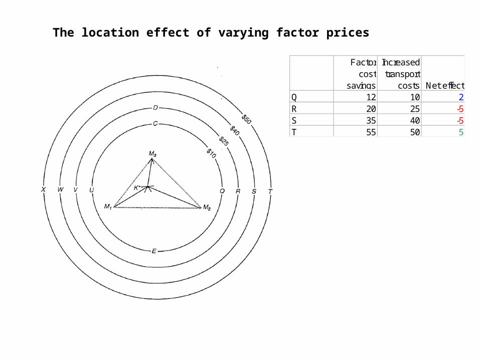
The location effect of varying factor prices
Factor cost
savings
Increased transport
costs Net effectQ 12 10 2R 20 25 -5S 35 40 -5T 55 50 5
Factor cost
savings
Increased transport
costs Net effectQ 12 10 2R 20 25 -5S 35 40 -5T 55 50 5
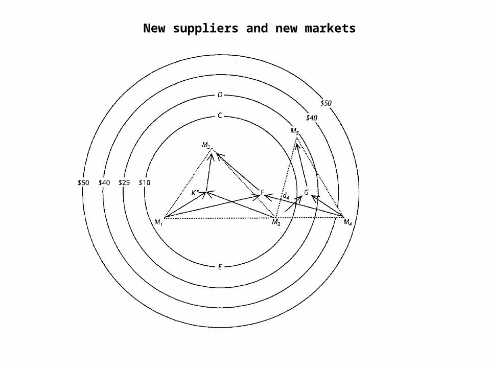
New suppliers and new markets
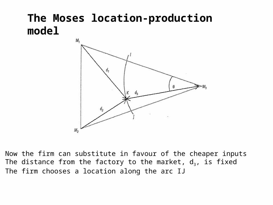
The Moses location-production model
- Now the firm can substitute in favour of the cheaper inputs- The distance from the factory to the market, d3, is fixed- The firm chooses a location along the arc IJ
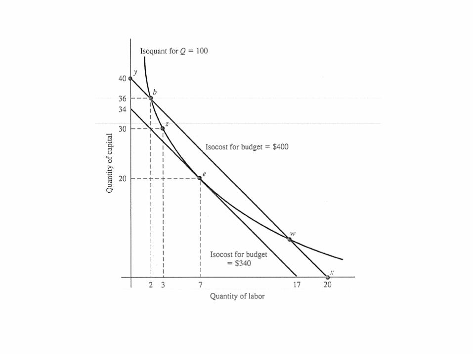

Budget constraints at the end points I and J
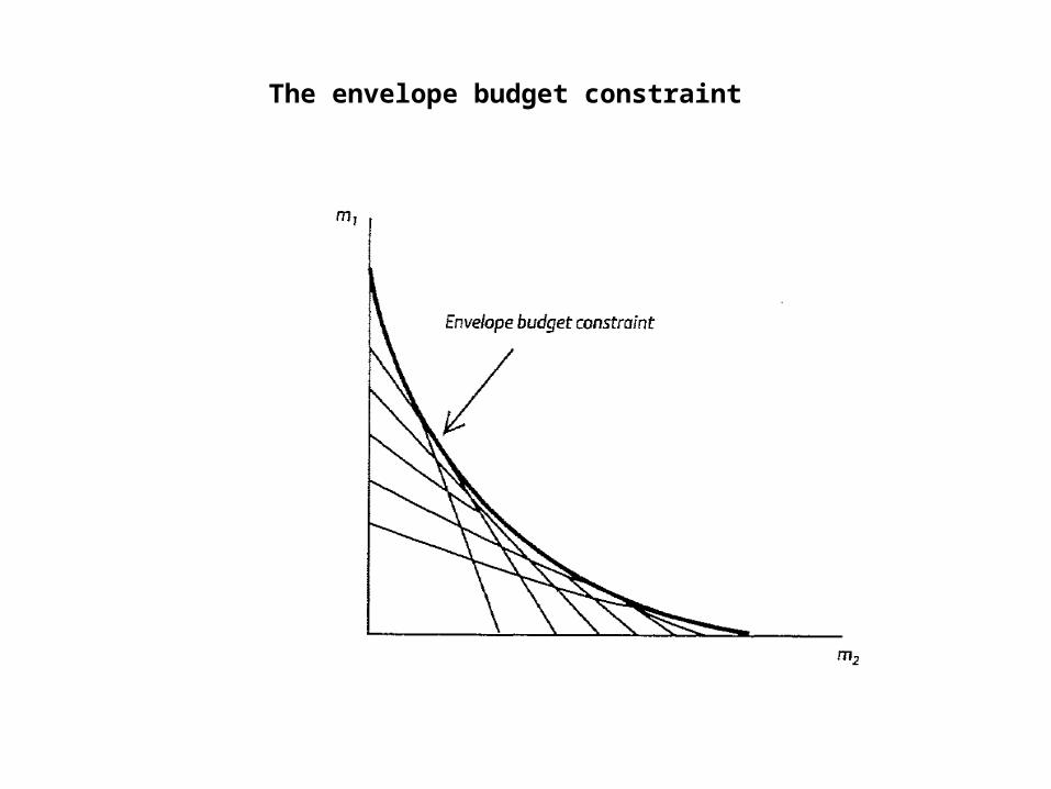
The envelope budget constraint

Location-production optimum

Effect of a road-building program that takes place in the area around M1

B. Location and market areas: Spatial monopoly
Spatial market areas: linear market with equal transport rates
Space can confer monopoly power on firmsThe lower transport and production cost are, the wider the monopoly area
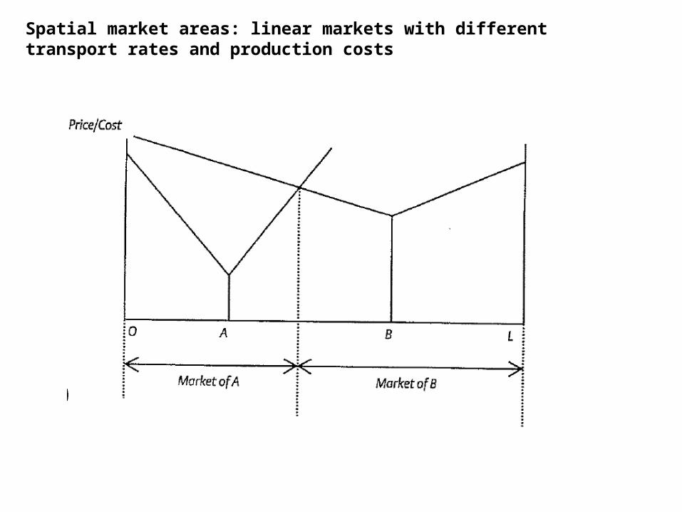
Spatial market areas: linear markets with different transport rates and production costs

C. Location and market areas: spatial competitionThe Hotelling location game
Assumptions1.Costless firm movement2. Homogenous product3. Consumers equally spaced along main street (i.e., sales are a + function of the market area)4. Perfectly inelastic demand5. Identical costs and transport rates

Welfare implications of the Hotelling result
Gain
LossLoss

Effect of price competition on the Hotelling result

• A firm lowers its price assuming that its rival’s prices will not change.
• Rival firm lowers its price assuming that the original firm will not change its price again.
• Etc.
• Every firm is surprised when the other firm retaliates.
• Result: Price shading continues until the firms price at or (temporarily) below MC
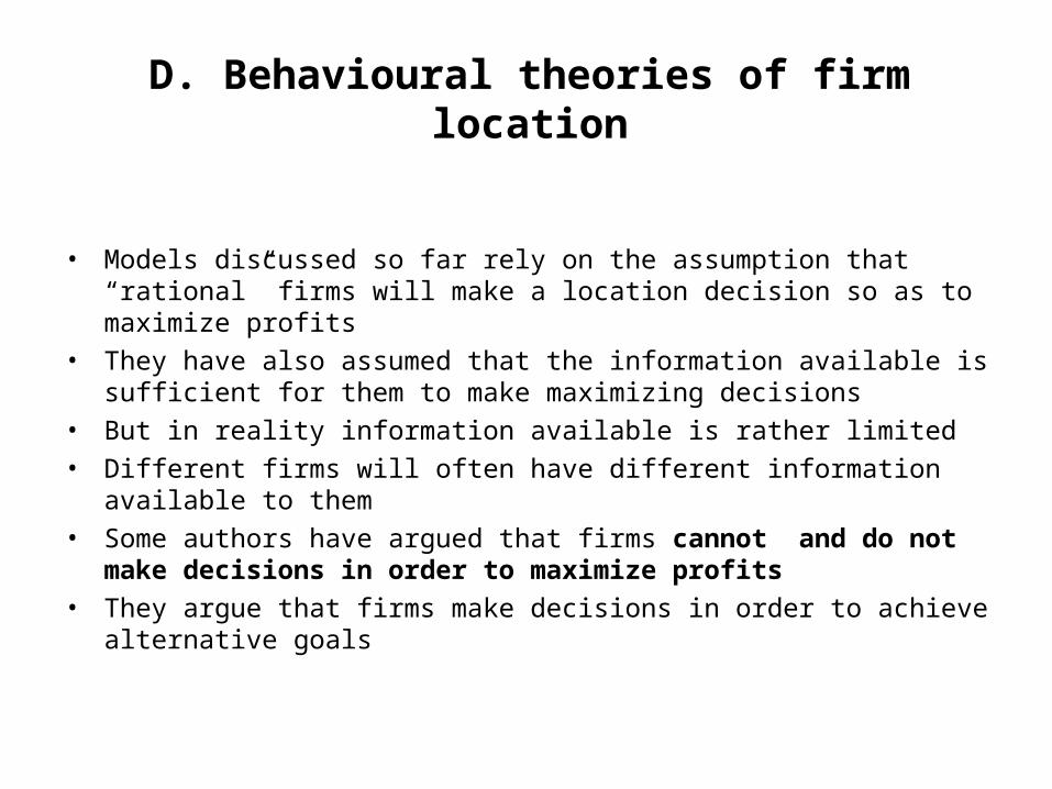
D. Behavioural theories of firm location
• Models discussed so far rely on the assumption that “rational” firms will make a location decision so as to maximize profits
• They have also assumed that the information available is sufficient for them to make maximizing decisions
• But in reality information available is rather limited
• Different firms will often have different information available to them
• Some authors have argued that firms cannot and do not make decisions in order to maximize profits
• They argue that firms make decisions in order to achieve alternative goals

• Critique has three themes:
1. Bounded rationality
2. Conflicting goals
3. Relocation costs
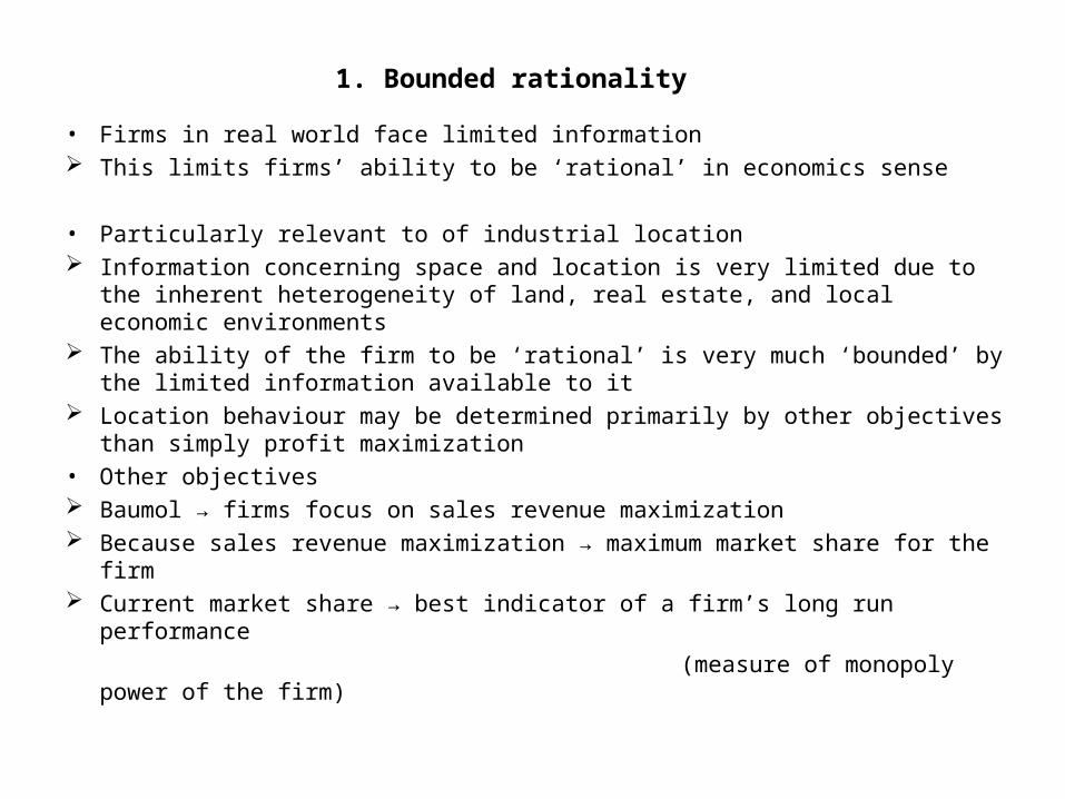
1. Bounded rationality
• Firms in real world face limited information This limits firms’ ability to be ‘rational’ in economics sense
• Particularly relevant to of industrial location Information concerning space and location is very limited due to the inherent
heterogeneity of land, real estate, and local economic environments The ability of the firm to be ‘rational’ is very much ‘bounded’ by the limited
information available to it Location behaviour may be determined primarily by other objectives than
simply profit maximization
• Other objectives Baumol → firms focus on sales revenue maximization Because sales revenue maximization → maximum market share for the firm Current market share → best indicator of a firm’s long run performance
(measure of monopoly power of the firm)
2. Conflicting goals
• Separation of ownership from decision-making
Different objectives are pursued
Corporate decisions are the result of many individual decisions made by a complex hierarchy
Performance of different employees within a company is measured in different ways
For example:
Director Firm’s market share
Sales manager Sales growth
Personnel manager Number of days lost through industrial disputes
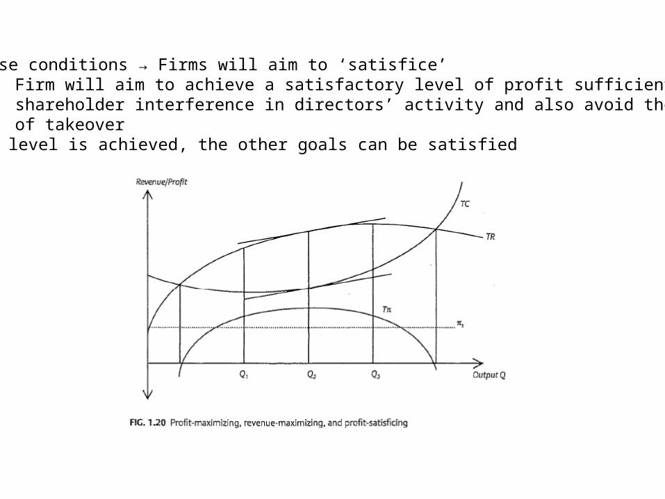
Under these conditions → Firms will aim to ‘satisfice’ Firm will aim to achieve a satisfactory level of profit sufficient to avoid shareholder interference in directors’ activity and also avoid the threat of takeover Once this level is achieved, the other goals can be satisfied

• From the point of view of location Firm aiming to maximize profits → P Firm aiming to maximize sales → S Firm aiming to minimize production costs → C
• If the firm had perfect information on cost and revenue spatial variation → P Given limited information and the conflicting goals actual location will depend on which is the particular dominant objective of the firm

3. Relocation costs
• Relocation costs → Costs incurred every time a firm relocates
• Previous models assume relocation costless But relocation costs can be high:
- Site search and acquisition
- Dismantling, moving, and reconstruction of existing facilities
- Construction of new facilities
- Hiring and training of new labour employed Firms are unlikely to move in response to small variations in factor prices or
revenues In conditions of imperfect information, bounded rationality, conflicting goals
and significant relocation costs → once a firm has chosen a location the firm will tend to maintain its location

• Behavioural approach is not prescriptive (do not indicate why a firm chooses a location in the first place)
• ¿How to interpret the previous models in the light of behavioural critique?
• Evolutionary argument of Alchian Behaviour of firms under uncertainty can be understood in relation to the
environment of the firm Environment → encompass all agents, information, and institutions
competing and collaborating in the particular set of markets in which the firm operates
Two types of environments:
- Adoptive
- Adaptive

Adoptive → ex-ante no firm has any particular information advantage over any other firms
‘Darwinian’ characterization: ex-post some firms will be successful while others will not
Adaptive → some firms are able to gather and analyse market information, simply by reason of their size
The probability of a particular firm making a profitable strategic decision is increased by reason of its size
Smaller firms will tend to perceive themselves to be at an information disadvantage
Strategy → make decisions which mimic those of larger firms (they know better market conditions)
• In terms of location Large firms → ‘rational decisions’ (they have the resources to evaluate the
cost and revenue implications of their location choice) Small firms will generally be located where their founders were initially
resident Over time, competition will be partly a result of spatial differences in costs
and revenues ¿location decision? In subsequent location decisions, small firms will tend to choose locations
close to the major market leaders (adaptive environment)

New manufacturing plants created in theinvestor’s “prior locality of economic activity”
Figueiredo et al (2002) case of Portugal
New manufacturing plants created outside theinvestor’s “prior locality of economic activity”


NEW ECONOMIC GEOGRAPHY
The Basic Idea
Typical story: economic activity will be concentrated in a core region,leaving only agricultural activity in the periphery.
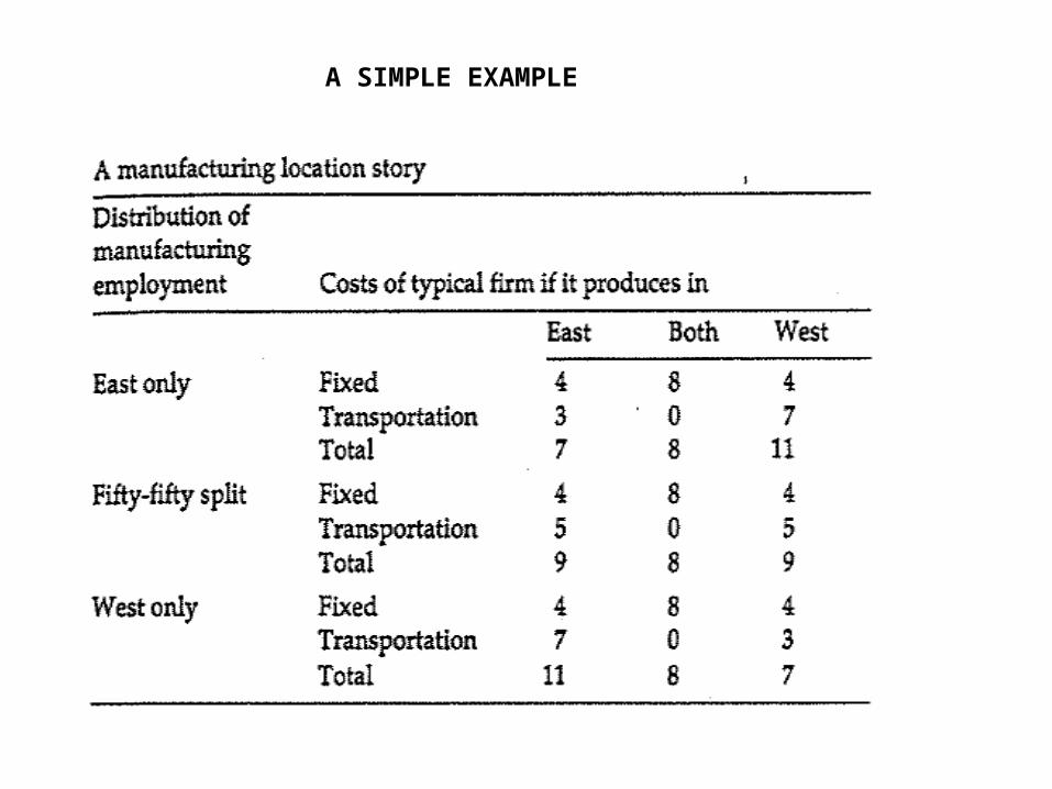
A SIMPLE EXAMPLE

Elements of the Core-Periphery Model
The core-periphery focuses on the location decisions of workers andfirms. It is a “2x2x2” model:
• 2 regions: North and South
• 2 inputs to the production process: Skilled labour and unskilled labour
• 2 products: A manufactured good and an agricultural product

The Agricultural Sector
• Agriculture is tied to land (traditional, CRTS, unskilled labor)
• Unskilled labor is assumed to be immobile
• Each region has a fixed amount of land and unskilled labor
• Transport cost (for agricultural goods) is zero.
The Manufacturing Sector
• Manufacturing is modeled as a modern production sector
• Goods are produced with skilled labor which is perfectly mobile between the two regions
• The modern sector with production subject to economies of scale
•The number of manufacturing firms is limited by increasing returns: manufactured goods are produced in factories, not in backyards.
Details of the Model
• Each manufacturing firm differentiates its product, producing one variety of the modern product
• Consumers exhibit preference for variety and balanced consumption
• Each consumer purchases at least a small quantity of each variety. (six varieties => each consumer buys from six firms)
• The bundle of products purchased by a consumer is determined by the relative prices of the varieties: the lower the price of a particular variety, the larger the quantity purchased.

Details of the Model (cont.)
• The prices of the varieties of the modern good are determined by competition and trade costs
• The larger the number of firms in a region, the more keen the competition among firms for consumers, and the lower the prices in that region
• The price of a variety imported from other region includes the cost of transporting the product (the trade cost), so imported varieties have higher prices than locally produced varieties: consumers buy larger quantities from local producers

The Symmetric Equilibrium
• Assume initially that we have symmetric regions, with an equal distribution of production between North and South
• Suppose there are six varieties produced by six firms, with the firms divided equally between the two regions
• North has firms {A, B, C}; South has firms {D, E, F}
• Local firms each sell the same quantity to home consumers. The non-local firms (e.g., firms D, E, F in North) mark up their prices to cover trade (transport) costs, so they sell less than the local firms
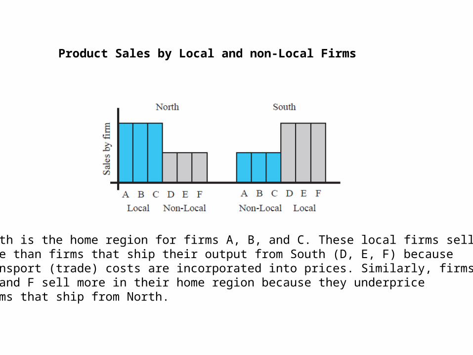
Product Sales by Local and non-Local Firms
North is the home region for firms A, B, and C. These local firms sellmore than firms that ship their output from South (D, E, F) becausetransport (trade) costs are incorporated into prices. Similarly, firms D,E, and F sell more in their home region because they underpricefirms that ship from North.

Symmetric Outcome
• “Equilibrium” implies no incentive for workers or firms to relocate
• Regions provide the same mix of modern varieties and the same average prices
• Consumers will reach the same utility level in both regions
• Wages are equalized
• Workforces are identical

Stability
• We are interested in whether the symmetric outcome is stable or unstable
• Test for stability: If a single firm were to relocate from South to North, what happens next?
• Two possibilities. 1. Self-Correcting Location Swap. 2. Self-Reinforcing Relocation.
Alternative Outcomes
1. Self-Correcting Location Swap. Relocation decreases profit a typical firm in the North and increases profits in South. Firms in the North then have an incentive to relocate, swapping places with the firm that originally moved from South to North.
2. Self-Reinforcing Relocation. Relocation increases profit of the typical North firm. Profits are higher in the North, and other firms from the South will have an incentive to relocate.

Local-Competition Effect of Relocation
Consider the effect of the relocation of a single firm (D) from South toNorth, from the standpoint of a firm in the North
• Good news: Sell more in the South.• Bad news: Sell less in the North. North firm will sell less in its home region because now there are four firms (up from three) who price their products without any trade cost markup.

Initial Equilibrium
Firms maximize profit by equating marginal revenue and marginalcost. This determines output per firm, whereas the number ofconsumers determines the number of firms in the market
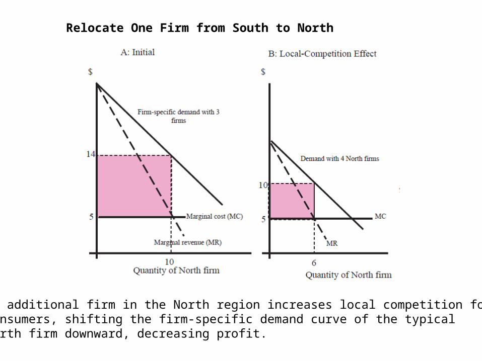
Relocate One Firm from South to North
An additional firm in the North region increases local competition forconsumers, shifting the firm-specific demand curve of the typicalNorth firm downward, decreasing profit.
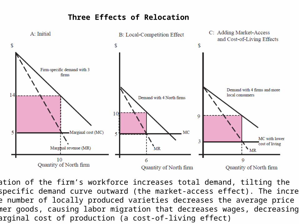
Three Effects of Relocation
Relocation of the firm’s workforce increases total demand, tilting thefirm-specific demand curve outward (the market-access effect). The increasein the number of locally produced varieties decreases the average price ofconsumer goods, causing labor migration that decreases wages, decreasingthe marginal cost of production (a cost-of-living effect)
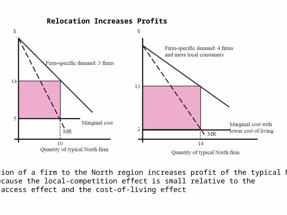
Relocation Increases Profits
Relocation of a firm to the North region increases profit of the typical Northfirm because the local-competition effect is small relative to themarket-access effect and the cost-of-living effect

Trade Openness and the Profit Gap
The local-competition effect decreases profit in the North and increases profitin the South. The market-access and cost-of-living effects increase profit inthe North and decrease profit in the South. All three effects diminish asopenness increases, reaching zero when trade is perfectly open (openness =1). The combined effect is negative when openness is low (f < f* ), butpositive when openness is high (f > f* ), and zero for perfect openness(f = 1).

Openness and Regional Divergence
When trade openness is low (f < f* ) ,the profit gap is negative, so thesymmetric outcome is stable (shownby solid line at north share = 1/2).When trade openness is high (f > f* ),the profit gap is positive, so thesymmetric outcome is unstable(shown by the dashed line for f > f* ).If relocation occurs from North toSouth, activity will be concentrated inthe North (shown by the solid line atNorth share = 1). Relocation in theopposite direction would causeconcentration in the South (shown bythe solid line at North share = 0).

Commuting Cost and Regional Divergence
Suppose the relocation of a firm to the North increases commuting distances and costs, increasing the wage paid to manufacturing workers. This effect shifts the profit-gap curve downward,so that the core-periphery outcomeoccurs for intermediate values of trade openness, between f* and f**

Evidence for the Core-Periphery Model
1. The core-periphery model is relatively new
2. Empirical results are mixed
3. Agglomerations of economic activity can be explained by a variety of theories
4. The core-periphery model predicts “catastrophic” changes in a regional economy, once a threshold degree of openness is crossed
5. The difficulty in policy applications of the model is that it is difficult to characterize what factors precipitate abrupt change

Measures of concentration• E = employment• s = ratio • i = sector i= 1,……., N• j = region j= 1,……., M• employment in sector i in region j
• total employement of region j • total employment of sector i
• total employment in the country
ijE
j iji
E E
i ijj
E E
iji j
E E

ijeij
j
Es
E i
i
Es
E
Coefficient of specialization
eij
i
s
sCoefficient of specialization of region j in sector i
ijcij
i
Es
E j
j
Es
E
Localization coefficient (or Hoover-Balassa)
cij
j
s
sCoefficient of localization of sector i in region j

Herfindhal index
2
1
( )n
e ej ij
i
H s
11,n
1
2e
j ij ii
IDEA s s
2
1
( )m
c ci ij
j
H s
11,m
1
2c
i ij jj
IDCA s s
Index of Isard
0,1
0,1
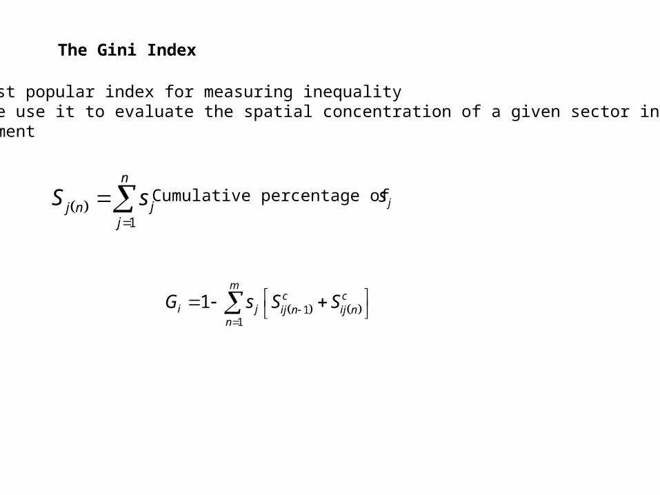
The Gini Index
The most popular index for measuring inequalityHere we use it to evaluate the spatial concentration of a given sector in terms of employment
1
n
jj nj
S s
Cumulative percentage of js
11
1m
c ci j ij n ij n
n
G s S S

cijs js
cij js s c
ijS jSRegion
1 0.1 0.2 0.5 0.1 0.2
2 0.2 0.25 0.8 0.3 0.45
3 0.3 0.25 1.2 0.6 0.7
4 0.4 0.3 1.3 1 1
1 ·1·1 0.52
ODCBAG
ODE
ODE
( )ODCBA ODE OAI ABGI BCFG CDEF
1 2x0.2x0.1OAI
1 2x(0.1+0.3)x(0.45-0.2)ABGI
1 2x(0.3+0.6)x(0.7-0.45)BCFG
1 2x(0.6+1)x(1-0.7)CDEF
0.5 0.4125 0.0875ODCBA
0.08750.175
0.5G
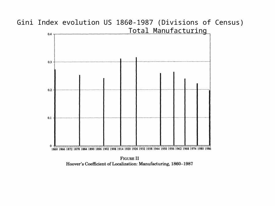
Gini Index evolution US 1860-1987 (Divisions of Census) Total Manufacturing
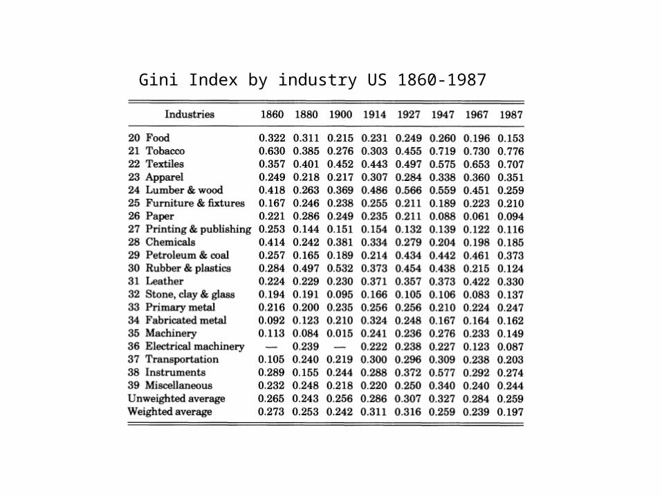
Gini Index by industry US 1860-1987