geoframe advanced petrophysical interpretation using...

Schlumberger ELANPlus GeoFrame Advanced Petrophysical Interpretation

ELANPlus GeoFrame Advanced Petrophysical Interpretation

Training and Exercise Guide

GeoFrame 4

1


Contents

Chapter 1 ElanPlus Introduction

Learning Objectives

Keywords

Overview

ElanPlus Equation Solutions

ElanPlus Quality Control

ElanPlus Benefits

ElanPlus Workflow

Chapter 2 Single Well ElanPlus Basic Features

Learning Objectives

Keywords

Exercise 2.1 Overview

Exercise 2.1: ElanPlus Basic Features

Parameter Calibration exercise (optional)

Model Builder

Chapter 3 Single Well ElanPlus Workflow

Learning Objectives

Keywords


Exercise 3.1: ElanPlus Workflow

Chapter 4 ElanPlus in Clastics Reservoir

Learning Objectives

Keywords


Exercise 4.1: Complex Clastic

Chapter 5 ElanPlus in Carbonate Reservoir

Learning Objectives

Keywords


Exercise 5.1: Vuggy Carbonate


Exercise 5.2: Complex Carbonate

Chapter 6 Multiwell ElanPlus Features

Learning Objectives

Keywords


Exercise 6.1: Parameter Creation and Zoning


Exercise 6.2:Multiwell Crossplot (Normalization)


Exercise 6.3: Multiwell Data Functioning


Exercise 6.4: Multiwell Presentation Display


Exercise 6.5: Multiwell Processing


Exercise 6.6: Missing Logs Estimation

Chapter 7 Reservoir Property Summation (ResSum) and Mapping

Learning Objectives

Keywords


Exercise 7.1: ResSum Workflow

2


3

About this course

This course explains how to use GeoFrame 4 petrophysics tools to process and interpret well logs. You will learn how to perform multi-mineralogical analysis on a single well or multiwell using ElanPlus.


4

Chapter 1 ElanPlus Introduction

Learning Objectives

After completing this course, you will be able to:

Understand the function of ElanPlus

Know the difference between ElanPlus and PetroViewPlus

Understand the workflow of running ElanPlus

Keywords

ElanPlus, Multimineral formation interpretation, Complex lithology, reconstructed log curve, PetroViewPlus, Workflow

Overview

ELAN is an abbreviation of “Elemental Analysis.” ElanPlus is the ELAN version in GeoFrame. ElanPlus provides level-by-level multi-mineral (complex lithology) quantitative formation evaluation with an optimized simultaneous equation solver and model combining method. The difference between ElanPlus and traditional petrophysical analysis methods (deterministic methods like PetroViewPlus) is that ElanPlus solves a set of equations (formed by logs, formation components volume and parameters) to derive the volume of each formation components first. Then calculates the formation properties (such as porosity, water saturation, volume of shale) from the derived volumes, not computes formation properties from a number of fixed formulas step-by-step like PetroViewPlus. The method used in ElanPlus can be illustrated by following figure:


5

Here, Vf means the total volume of fluids in formation; Vw means the total volume of water in formation.

ElanPlus Equation Solutions

Because of the complex relationship between formation properties and log measurements, the petrophysical interpretation will experience three cases in providing reasonable solutions for multimineral formation evaluation. These are: determined equations (if number of formation components is equal to the number of log measurements plus one); underdetermined equations (if number of formation components is more than the number of log measurements plus one); and over-determined equations (if number of formation components is less than number of log measurements plus one). ElanPlus can provide the best solutions for these three types of equations by introducing the concept of constant tool/external tool/constraint/uncertainty/user-defined information and model combining to integrate local geological knowledge and user’s experience with mathematics solutions. The different solutions covered by ElanPlus can be explained by the following figure:


6

ElanPlus Quality Control

For each volumetric solution, ElanPlus will also output reconstructed logs based on the model, the reconstructed logs are very important when validating results or creating artificial logs. Reconstructed logs allow for better quality control and parameter adjustment.

ElanPlus Benefits

One of the main benefits of ElanPlus is the ability to customize the formation model (Solver) to match the local mineralogy to produce a more accurate representation of the rock, both in terms of lithology and petrophysical properties. In addition, ElanPlus allows multiple models (Solver and Combine), parameter calibration (ParCal), and reconstructed logs, as for more information in detailed on ElanPlus theory and features (constraint expression, probability expression, constant tool expression, uncertainty expression, special response equation and saturation equation) please refer to the Online Help Documentation from GeoFrame Bookshelf.

ElanPlus Workflow

GeoFrame ElanPlus has both single well mode and multiwell mode, also shares information with other applications through a common project database. The typical workflow of ElanPlus in GeoFrame can be illustrated by the following figure:


7


8

Chapter 2 Single Well ElanPlus Basic Features

Learning Objectives

After completing this course, you will be able to

Understand the basic features of ElanPlus

Know how to build ElanPlus Solve model

Know how to set parameters for interpretation

Know how to write constant tool expression

Know how to write constraint expression

Understand the balanced uncertainty

Know how to combine the model

Know how to write model probability expression

Know how to use Function model

Understand the parameter calibration function (ParCal)

Keywords

ElanPlus, Solve, Combine, Function, ParCal, Constant Tool, Constraint, Probability, Balanced uncertainty, Parameter initialization, Volume, Equation, Linear, Non-linear, Mineral, Fluid, Formation component


Data Requirement

In order to get a reasonable solution for the reservoir you are working with, you need to get a complete suite of wireline logs data, core measurement data and geology report. Before you build the petrophysical interpretation model, it is very important for you to investigate the geological information from the core data and geology report.

Basic Features Overview

The purpose of next exercise is to help you have a good understanding of basic features of ElanPlus, including:

How to load log data and core data (Data Load and ASCII Load)

How to Build Simple ElanPlus interpretation model (Process, Parameter, Channel)

How to calculate the zone parameter (Initialize Parameters)


9

How to compute logs Uncertainty and adjust Weight factor

How to use Constant tool (CT1, CT2…)

How to write Constraint expression for your interpretation model

How to combine the ElanPlus interpretation model (Solve, Combine, Dependency)

How to write model combination probability expression

How to compute porosity, saturation and permeability (Fun Process)

Exercise 2.1: ElanPlus Basic Features

Please Note: Document conventions regarding the mouse.

MB1: Mouse Button 1 (Left Mouse Button). The default instruction to “Click…” is to select, highlight, or activate the item using MB1

MB2: Mouse Button 2 (Middle Mouse Button)

MB3: Mouse Button 3 (Right Mouse Button)

Data Loading

(If the data has been loaded into GeoFrame, please skip step 1 to 5)

1. From the Application Manager window, click (MB1) the Data icon to open Data Management window.


10

2. From Data Management window, open the Loaders and Unloaders folder.

3. Select Data Load module, and click OK to run the data loading module by:


11

File name: (your instructor will tell you what it is)/merlin.dlis

Field: Merlin

Well UWI: Merlin

Borehole UWI: Merlin

Producer: Schlumberger

4. Click Run to load the data and exit from data loading window after competed.

5. Click OK for all the confirmation windows.

Start ElanPlus from the Process Manager

6. From the Application Manager window, click the Process icon to open the Process Manager.

7. From Process Manager, put a ElanPlus module into the Process Manager by:


12

Click the icon to open the Product Catalog.

Select Petrophysics from the Product Catalog to open the petrophysics product list.

Select the ElanPlus module and click OK.

8. From the Process Manager window, set Data Focus for ElanPlus module by:

Click the icon to open the Data Focus Selection window.

From Data Focus Selection window, highlight the project name, if it is not highlighted.

Change Show menu to Borehole (Click on Show to make the change).

Select only the Merlin borehole and click OK.

9. From the Process Manager window, click the Activity button to rename your activity (just type in a new meaningful name for your activity, for example: Basic ElanPlus interpretation).

10. Double-click on the ElanPlus icon from the Process Manager to open ElanPlus Session Manager. If the Multi ElanPlus Session Manager is open, go to menu User to select Single Well Mode to open ElanPlus Session Manager.


13

Build a Reservoir Model

1) From ElanPlus Session Manager window, click the icon to open a SOLVE (S1) model to compute volumes from input logs.


14

2) For the model icon in the drawing area, you can move, select, or unselect it by:

Moving a model icon: Click on it with MB2, hold down the button while dragging the model icon wherever you want it, and then release MB2. The icon will move to wherever the mouse cursor was when you released the mouse button, and any dependencies connected to it will move along with it.

Selecting a single model icon: Click on the icon with MB1, the icon will change to reverse video.

Selecting Multiple model icons: To select two or more model icons at once, press the <Ctrl> key or the <Shift> key (from the keyboard) and hold it while clicking on each of the icons. Then release the <Ctrl> or <Shift> key.

Unselecting a model icon: Click on any blank part of the Drawing Area or click on any other model icon, the model icon will no longer be black.

3) Move the SOLVE (S1) icon to a position you wish to place it (See step 7 on how to move it)

4) For the model icon in the Drawing area, you can rename it to a name you like by:

Click on the model icon to select it

Click and hold down MB3 on the selected model icon until a Process menu appears.

Select the Rename Process option from the menu, a Rename Process window will appear

In the Rename Process window, highlight the existing process name (by dragging the mouse over it in the Process Name field), and then type in the new process (model) name.


15

Click the OK button, to save your new process name and to close the Rename Process window.

11. Rename, changing the SOLVE (S1) to Reservoir (See Step 9 on how to rename it)

12. Double-click on the Reservoir (S1) icon to open the Solve Process Editor (Edit Reservoir (S1))

13. From the Solve Process Editor, you can select Volumes you wish to use to build your ElanPlus interpretation model by:

Click on the menu box at the top left corner and hold down to select Volume (it maybe shows as Volume, Equation, or Constraint before you make a selection).

Click on the menu box under the Volume items list box to select Minerals (it may show as Minerals, Rocks, or Fluids before you make a selection). Then you select what mineral you wish to use, and click the right-pointing arrow button beside the list. The mineral you selected will appear in the Volumes list panel.

Click on the menu box under the Volume items list box to select Rocks (it may show as Minerals, Rocks, or Fluids before you make a selection). Then, select what rock you wish to use, and click on the right-pointing arrow button beside the list. The rock you selected will appear in the Volumes list panel.

Click on the menu box under the Volume items list box to select Fluids (it may show as Minerals, Rocks, or Fluids before you make a selection). Then, you select what fluid you wish to use, and click on the right-pointing arrow button beside the list. The fluid you selected will appear in the Volumes list panel.

You can remove the Volume from the Volumes panel by clicking the item you wish to remove, and then click the left-pointing arrow to remove it.

You can make multi-volume selection by holding down the <Ctrl> key, while clicking on each of the volume items, then release the <Ctrl> key.


16

14. From the Solve Process Editor, you can select Equations that you wish to use to build your ElanPlus interpretation model:

Click the menu box at the top-left corner and hold down to select Equation (it may show as Volume, Equation, or Constraint before you make a selection).

Click the menu box under the Equation items list box to select Linear (it may show as Linear, Non-linear, User Definable, or Geochemical before you make a selection). Then you select what linear equation (GR, RHOB) you wish to use, and click the right-pointing arrow button beside the list. The linear equation you selected will appear in the Equations list panel.

Click the menu box under the Equation items list box to select Non-linear (it may show as Linear, Non-linear, User Definable, or Geochemical before you make a selection). Then you select what non-linear equation (CUDC_DWA, CXDC_DWA) you wish to use, and click the right-pointing arrow button beside the list. The non-linear equation you selected will appear in the Equations list panel.

Click the menu box under the Equation items list box to select User Definable (it may show as Linear, Non-linear, User Definable, or Geochemical before you make a selection). Then you select what User-defined equation (constant tool CT1, CT2…) you wish to use, and click the right-pointing arrow button beside the list. The constant tool you selected will appear in the Equations list panel.

Click the menu box under the Equation items list box to select Geochemical (it may show as Linear, Non-linear, User Definable, or Geochemical before you make a selection). Then, you select what geochemical equation (WWK, WWTH) you wish to use, and click the right-pointing arrow button beside the list. The Geochemical equation you selected will appear in the Equations list panel.

You can remove the Equation from the Equations panel by clicking on the item you wish to remove, and then click the left-pointing arrow to remove it.

You can make multi-equation selection by pressing the <Ctrl> key and holding it while clicking on each of the equation items, then release the <Ctrl> key.

15. From the Solve Process Editor, you can select existing Constraints you wish to use, or define the new Constraint expression, to build your ElanPlus interpretation model by:

Click the menu box at the top-left corner and hold down to select Constraint (it may show as Volume, Equation, or Constraint before you make a selection).

The pre-built Constraints list will be displayed in the box below Constraint, you can select the Constraint you wish to use, and click the right-pointing arrow button beside the list. The Constraint you selected will appear in the Constraints list panel

Below the Constraint item list box is an Edit button. Click the Edit button, and the Constraints Editor window will appear. It is a simple text editor, in which you type the text expression for the new constraint

After you create a new constraint, the constraint’s name will appear in the Constraint items list box. You select it, and click on the right-pointing arrow button beside the list. The Constraint you created will appear in the Constraints list panel.

16. From the Edit Reservoir 1 Editor window, select the following Volumes (see Step 12 for help):

QUAR

ILLI


17

XWAT

UWAT

XGAS

UGAS

17. From the Edit Reservoir 1 window, select the following Equations (see step 13 for help)

GR

RHOB

CXDC

CUDC

18. Toggle ON (turn to red) both of the small square buttons for Volume and Logs (beside Auto Display:).

19. Click OK to close this window.

20. Click the icon to check the Channel Binding.


18

21. Click the icon to open the Zone Parameter Editor window.

22. In the Zone Parameter Editor window, set up zone parameters by:


19

Set Grouped By to Equations. Use MB1 to click the small box menu on the top left of the window and hold down to make the selection.

Toggle ON Use Equations vs. Volumes Format. Use MB1 to click on the small square button beside Equations vs. Volumes Format to turn it to Red.

Set Visibility Setting option from Standard to All. Use MB1 to click on the small box menu with Standard and hold down to make your selection.

Click the Select All button under the top-left Equation items list panel, and then click on button Refresh on the bottom of this window.

Click the Initialize Parameters… button to open Parameter Initialization window.

23. From the Parameter Initialization window, you can initialize salinity-dependent parameters by:

Enter RW/RWT (or SALIN_UWAT), RMF/MST (or SALIN_XWAT), TVD, Mud weight, Average Porosity, and Zone reference temperature.

Click the Compute button in the upper right-hand corner of the window. The program then computes the salinity and temperature-dependent parameters and gas-dependent parameters.

Click OK to apply the computed parameters and update your zone parameters.

24. Check and modify the response parameters based on the following table:


20

25. Set following parameters in the Parameter Initialization window and compute the parameters for this example (see step 20 for help):

SALIN_UWAT=200 ppk SALIN_XWAT=180.1 ppk

Zone Temperature = 141° C (285° F)

Mud Weight = 1.2 g/cm3 (10 lb/gal)

Average Porosity = 0.15

26. Click on Compute and then click on OK to close this window

27. Click the icon in the Zone Parameter Editor window to run the application. Check the overlay and separation between the reconstructed curve (solid line) and input log curve (dashed line) to ensure you are happy with the interpretation from the display.

28. Try to adjust the parameters, and answer the following questions:

You want to increase clay volume in shales. Which parameter is most sensitive?

You want to decrease clay volume in sands. Which parameter is most sensitive?

You want to increase XWAT volume in sands. Which parameter is most sensitive?

You want more Gas. Which parameter is most sensitive?

No matter how you adjust the parameters, the curve’s overlay in some depth interval is still poor. Why? (We will answer this question in exercise 2).

29. Click on OK button from Zone Parameter Editor window to close it.

How to compute and adjust CUDC and CXDC Uncertainties



21

31. In the Zone Parameter Editor window, set up Uncertainties parameters by:

Set Grouped By to Uncertainty. Use MB1 to click on the small box menu on the top left of the corner, and hold MB1 down to make the selection).

Select CUDC_UNC_ZP and CXDC_UNC_ZP from the list, compute these parameters by: CUDC_UNC_ZP = sqrt (CUDC_UWAT/1000. -CUDC_QUAR/1000.) *0.015 *1000.

CXDC_UNC_ZP = sqrt (CXDC_XWAT/1000. -CXDC_QUAR/1000.) *0.015 *1000.

For this example: CUDC_UNC_ZP = 132 and CXDC_UNC_ZP = 127.

32. Reset these two parameters, and click the icon to run the application.


22

33. Go to menu File > Close to close this graphics window.

34. Click OK from Zone Parameter Editor window to close it.

How to Write a Constraint Statement from the Local Knowledge

If there is some local geological information, that for this borehole the Porosity should be smaller than 18%, and Clay volume should be less than 85%, how you will use these information as a constraint – to match your final interpretation with the local geological knowledge.

Select Reservoir S1 and hold down MB3 to select Edit Process… to open Edit Reservoir 1 window.


23

From Edit Reservoir 1 window, select a existing constraint and create a new constraint (see step 14 for help)

Select Maximum Porosity from the Constraint list and move it to the Constraints panel

Click Edit to open the Constraint Editor window and write the following constraint expression (you can go to menu Help to get online help for writing constraint):

Constraint (Max_shale_volume, ILLI < = 0.85)

Click on button Check to see if there are syntax errors, if there are no errors, click OK to close the Constraint Editor window, and the Constraint named Max_shale_volume will come into the Constraint list box

Select Max_shale_volume from the Constraint list and move it to the Constraints panel


24

Click OK to close the Edit Reservoir 1 window.


36. In the Zone Parameter Editor window, set up All parameters by:

Set Grouped By to All (use MB1 to click on the small box menu on the top left of the corner and hold down to make the selection).

Scroll the list down to select PHIMAX, WCLP_CLA1 and WCLP_CLA2 and click the button Refresh, then set the parameters as: PHIMAX=0.18, WCLP_CLA1=0.156 and WCLP_CLA2=0.156.


25

Click the icon to run the application and check the display to see how the constraints work for your interpretation.

Click Cancel to close the Zone Parameter Editor.

37. In the ElanPlus Session Manager, double-click on Reservoir S1 model icon to open the Edit Reservoir 1 window. From this window, remove constraints from the Constraints panel (see step 14 for help if needed).

38. Click OK to close the Edit Reservoir 1 window.

How to Write a Constant Tool Statement

If the Rxo (CXDC) data is bad, you cannot use CXDC data to compute XGAS, but there is a local geological knowledge known, that XGAS/UGAS = 20%. Here is how to use this information as the constant tool to do your interpretation.

39. From the ElanPlus Session Manager, double-click on Reservoir S1 model icon to open the Edit Reservoir 1 window, from this window, remove equation CXDC from The Equations panel (see step 13 for help if needed)


26

40. From the Edit Reservoir 1 window, add Constant Tool CT1 from the Equation list to the Equations panel (see step 13 for help if needed), then click OK to close the Edit Reservoir 1 window.


42. In the Zone Parameter Editor window, set up zone Equation parameters by:


27

Set Grouped By to Equation. Use MB1 to click on the small box menu on the top left of the corner and hold down to make the selection.

Click on button Select All and the press on button Refresh

Set the parameters for CT1 based on the following pseudo-equation:

XGAS/UGAS=0.2 ----

XGAS=0.2*UGAS ---

0=0.2*UGAS-1*XGAS --

0=0.2*UGAS-1*XGAS+0*UWAT+0*XWAT+0*ILLI+0*QUAR

So:

CT1_UGAS=0.2, CT1_XGAS=-1 and the rest of CT1 parameters are 0

Change the Grouped By from Equation to Uncertainty and select CT1_UNC_ZP and CT1_UNC_WM from the list. Click the Refresh button, and set the parameters like this: CT1_UNC_ZP=0.015 and CT1_UNC_WM = 1.

Click the icon to run the application and check the display to see how the constant tool CT1 works for your interpretation.


28

Go to File > Close to close this graphic window.

Click the Cancel button to close the Zone Parameter Editor.

Build a Model to Solve for Anhydrite

From ElanPlus Session Manager window, click the icon to open a SOLVE (S2) model to compute Anhydrite volumes from input logs.

43. Move the SOLVE (S2) icon to the right of Reservoir (S1) icon (See step 7 on how to move it).

44. Rename the SOLVE (S2) to Anhydrite (See Step 9 on how to rename it).


29

45. Double-click on the Anhydrite (S2) icon to open the Solve Process Editor (Edit > Anhydrite (S2).

46. From the Edit Anhydrite 2 Editor window, select the following Volumes (see Step 12 for help).

CALC

DOLO

ANHY

ILLI

XWAT

47. From the Edit Anhydrite 2 window, select the following Equations (see step 13 for help)

RHOB

NPHI

U

GR

48. Toggle ON the small square button on the left side of Volume and Logs beside Auto Display toggles below the list areas in the center of the window, click on OK to close this window


30

49. Click on the icon to open the Zone Parameter Editor window


Set Grouped By to Equations. Use MB1 to click on the small box menu on the top left of the corner and hold down to make the selection.

Toggle on Use Equations vs. Volumes Format. Use MB1 to click on the small square button beside “Equations vs. Volumes Format” to turn it to Red

Set Visibility Setting option from Standard to All. Use MB1 to click on the small box menu with Standard or All and hold down to make your selection.

Click on button Select All under the top-left Equation items list panel, and then click on button Refresh on the bottom of this window

Click on button Initialize Parameters… to open Parameter Initialization window.

51. From the Parameter Initialization window, you can initialize salinity-dependent parameters by:

Enter RW/RWT (or SALIN_UWAT), RMF/MST (or SALIN_XWAT), TVD, Mud weight, Average Porosity and Zone reference temperature

Click on the Compute button in the upper right-hand corner of the window, the program then compute the salinity and temperature-dependent parameters and gas-dependent parameters

Click OK button to apply the computed parameters and update your zone parameters

52. Check and modify the response parameters based on the following table:


31

53. Set following parameters in the Parameter Initialization window and compute the parameters for this example (see step 53 for help):


Zone Temperature=141° C (285° F)

Mud Weight=1.2 g/cm3 (10 lb/gal)

Average Porosity=0.05

Click Compute and then click OK to close this window.

54. Click the in the Zone Parameter Editor window to run the application, check the overlay/separation between the reconstructed curve (solid line) and input log curve (dashed line) to see if you are happy with the interpretation from the display

55. Click on Cancel to close the Zone Parameter Editor window

Build a Shale/Badhole Model

56. From ElanPlus Session Manager window, click the icon to open a SOLVE (S3) model icon to compute Shale volumes from input logs.

57. Move the SOLVE (S3) icon to the right of Anhydrite (S2) icon.

58. Rename the SOLVE (S3) to Shale.


32

59. Double-click on the Shale (S3) icon to open the Solve Process Editor (Edit > Shale (S3).

60. From the Edit Shale 3 Editor window, select the following Volumes: QUAR and SHAL.

61. From the Edit Shale 3 window, select the following Equation: GR.

62. Toggle ON Volume and Logs, and then click OK to close this window.


33

63. Click (MB1) on the icon to open the Zone Parameter Editor window


Set Grouped By to Equations (use MB1 to click on the small box menu on the top left of the corner and hold down to make the selection)

Toggle on Use Equations vs. Volumes Format (use MB1 to click on the small square button beside “Equations vs. Volumes Format” to turn it to Red)

Set Visibility Setting option from Standard to All (use MB1 to click on the small box menu with All or Standard and hold down to make your selection)

Click on button Select All under the top-left Equation items list panel, and then click on button Refresh on the bottom of this window

65. Check and modify the response parameters as below:

GR_SHAL=150 GR_QUAR=20

66. Click the icon in the Zone Parameter Editor window to run the application, check the overlay/separation between the reconstructed curve (solid line) and input log curve (dashed line) to see if you are happy with the interpretation from the display

67. Click on Cancel to close the Zone Parameter Editor window


34

Combine the Models

Now you have three models for your interpretation, you need to output a reasonable interpretation by combining these three models. There are two ways to make model combination:

Insert a new zone above14826 ft (4520 m) and let the final interpretation coming from Anhydrite model

Below the depth 14826 ft (4520 m), let the final interpretation coming from the internal average of the model probability, the model switch on the probability which will be calculated by:

If the clay volume of Reservoir model exceeds 55%, the final interpretation will come from Shale model;

If the clay volume of Reservoir model is less than 45%, the final interpretation will come from Reservoir model;

If the clay volume of Reservoir model is between 45% and 55%, the final interpretation will come from the linear interpolation average of both Reservoir model and Shale model, the linear interpolation expression looks like:

shale=linear(ILLI_VOL.SOL.1,0.45,0.,0.55,1.)

prob (SOL.3, shale)

That means:

p3 = prob (SOL.3, shale) — the probability of model 3 is p3

p3 = 0 if ILLI_VOL.SOL.1< = 0.45

p3 = 1 if ILLI_VOL.SOL.1 > = 0.55

p3 = ILLI_VOL.SOL.1*10-4.5 if 0.45 < = ILLI_VOL.SOL.1 < = 0.55

p1 = (1-p3)

Vj = Σpi*Vij (i = 1, model number, j = 1, volume number)

1. From the ElanPlus Session Manager, click the icon to open a COMBINE model icon, move it under the Reservoir (S1), Anhydrite (S2) and Shale (S3) (see step 7 for help if needed)


35

2. From the ElanPlus Session Manager, you can define the relationships between models, to specify a dependency, do this:

Activate the Dependency Tool by clicking on the Dependencies (diagonal arrow) icon

Click on (MB1) the source model icon, connecting the source model and the cursor will appear a sort of rubber band line that stretches between them no matter where you move the cursor in the Drawing Area

Click on (MB1) the destination model, when you release the mouse button, the rubber band becomes a arrow pointing from the first model to the second, indicating the dependency

You can use MB3 to delete the rubber band line (dependency) if you made a mistake

3. Define dependency between Reservoir (S1) and COMBINE, Anhydrite (S2) and COMBINE, Shale (S3) and COMBINE (see step 66 for help)

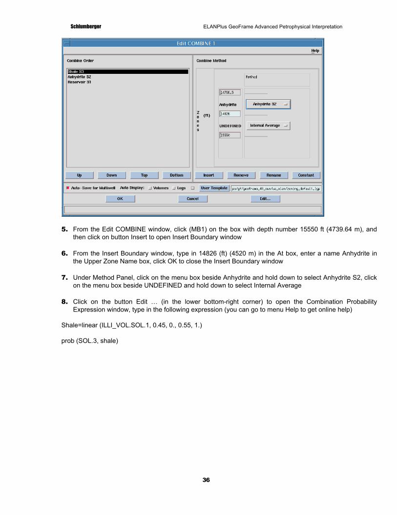
4. Double-click on COMBINE model icon to open the Edit COMBINE window


36

5. From the Edit COMBINE window, click (MB1) on the box with depth number 15550 ft (4739.64 m), and then click on button Insert to open Insert Boundary window

6. From the Insert Boundary window, type in 14826 (ft) (4520 m) in the At box, enter a name Anhydrite in the Upper Zone Name box, click OK to close the Insert Boundary window

7. Under Method Panel, click on the menu box beside Anhydrite and hold down to select Anhydrite S2, click on the menu box beside UNDEFINED and hold down to select Internal Average

8. Click on the button Edit … (in the lower bottom-right corner) to open the Combination Probability Expression window, type in the following expression (you can go to menu Help to get online help)

Shale=linear (ILLI_VOL.SOL.1, 0.45, 0., 0.55, 1.)

prob (SOL.3, shale)


37

9. Click on Check to see if there are any errors, if no errors, click on Close to exit this window

10. Toggle on the small square button on the left side of Volume and Logs beside Auto Display toggles below the list areas in the center of the window, click on OK to close this window

11. Click the icon to run the application (if there is a warning message said that COMBINE: All previous processes must be executed, click OK to close this warning window, then go to menu Edit >

Select All to select all of the models and then click the icon to run the application)


38

12. If you want to change the display option, go to menu Output > Display to make your display selection


39

Compute Porosity, Saturation etc. Properties from Function Model

1. From the ElanPlus Session Manager, click the icon to open a Function model icon, move it under the COMBINE model (see step 7 for help if needed)

2. Define dependency between COMBINE and Function (see step 66 for help)

3. Double-click on Function model icon to open the Edit FUNCTION window


40

4. From the Edit FUNCTION window, select PIGN RHGA SUWI and SXWI from the Available Functions panel and move them to the Selected Functions Panel by clicking on the right-pointing arrow

5. Toggle ON Petrophysics option for Autodisplay, click OK to exit from this window

6. Click the icon to run the application, check the results from the display


41

7. If you are happy with the results, close the display window by File > Close

8. From ElanPlus Session Manager window, go to menu File > Save as to save your job as a session file (with .elp as the extension for the file name)


42

9. If you like, go to menu File > Save Output to save results into GeoFrame Database.

Parameter Calibration Exercise (Optional)

From the ElanPlus, you can use ParCal to calculate response parameters from input volumes and log tool measurements

1. Go back and recall the interpretation activity you did for Merlin and inspect ElanPlus

2. Place a PARCAL process in the ElanPlus graphical area by clicking on the icon called PARCAL. Move this process under the main Reservoir solve process.

3. Create a dependency from the Reservoir solve process to the PARCAL process using the arrow

icon.


43

4. Edit the PARCAL process. Since PARCAL calculates response parameters from input volumes and tool measurements, you will see the volumes list from the Reservoir (Solver) process already available in the PARCAL process.

5. We are going to use PARCAL to calculate the sonic response for the Clay (Illite) and the Quartz, assuming that our Reservoir model has created good volumes.

6. Select QUAR and ILLI in the volumes list and toggle the “Calibrate” option button below the list. You should see a > symbol appear to the left of QUAR and ILLI in the list. This indicates that only response parameters for these volumes will be calculated.

7. Select DT from the linear equations list, and click the “Bind input” toggle. If an * does not appear beside the DT equation, then you will need to bind a DT curve for the PARCAL process using the Edit > Channels window.


44

8. Set the Auto Display for both Logs and Volumes. Click OK for the PARCAL window.

9. Now click icon to edit Parameters for the PARCAL process. Notice that the only response parameters to edit are DT parameters. Click in the box where you would normally enter the DT_ILLI parameter, and notice that the box at the bottom is requesting a Tolerance for DT_ILLI. Type in 35 us/ft for the Tolerance of DT_ILLI - you MUST type this number in the box at the bottom. Now click in the DT_QUAR text field, and then set a tolerance of 35 us/ft for the tolerance of DT_QUAR.


45

10. Other PARCAL parameters are accessed by toggling the top left option button to All, and then scrolling down the list, You will see these parameters:

• SDRMAX: Threshold for maximum reduced coherence. IF SDR is greater than (>) SDRMAX then PARCAL will skip this level for processing.

• VOLMIN: Minimum volume threshold for calibration. If a volume whose response parameter is being calculated goes below VOLMIN, then PARCAL skips this level.

• TCVOLS: Tolerance on summation of volumes = 100%.

• MDCS: Maximum delta caliper threshold.

• PARCAL1_ST: First calibration zone set status. 1 = calibrate, 0 = do not calibrate.

11. Run the ParCal process by . The automatic display shows how well DT reconstructs with ParCal’s new values (DT_QUAR and DT_ILLI). To see what PARCAL calculated for the new response parameters, go to Output > PARCAL Parameters in the ElanPlus Session Manager window. The calibrated parameters are color-coded; Green for calibrated, Red for limited by the parameter tolerance. These new PARCAL parameters can now be put back into the solve process if desired.


46

Model Builder

If you want to build an ElanPlus model via Model Builder provided by ElanPlus, just click the icon, the Model Builder interface will come up, and you can work with it item by item to build an ElanPlus interpretation model.


47

Chapter 3 Single Well ElanPlus Workflow

Learning Objectives

After completing this course, you are able to

Understand the importance of knowing the geological background to using ElanPlus

Know how to use WellCompositePlus and Crossplot tools to investigate lithology

Know how to use crossplot from ElanPlus to study the clay type

Build a more reasonable ElanPlus interpretation model

Keywords

Lithology, WellCompositePlus, Utility Plots, Crossplot, ElanPlus model, Lithology investigation, Interaction


Lithology Investigation by WellCompositePlus and UtilityPlots

Before you work with ElanPlus application, try to use WellCompositePlus and UtilityPlots to investigate the lithology and other geological information for the borehole data you will do the interpretation.

Petrophysical Interpretation Model Building

Base on the information you get from geology report, core data and lithology investigation from WellCompositePlus and UtilityPlots, then you start to work with ElanPlus to build the correct petrophysical interpretation model (geological model and parameters)

Exercise 3.1: ElanPlus Workflow

The purpose of next exercise is to help you have a good understanding of advanced features of ElanPlus, including:

How important that a proper geological model will simplify your interpretation (answer last question from Exercise 1)

The ability that ElanPlus can handle for complex lithology petrophysical interpretation

Quality control your interpretation from the reconstructed curve overlay with input curve (if the borehole is good)

Start a new activity from Process Manager by creating a process chain with 3 applications: WellCompositePlus, UtilityPlots and ElanPlus


48

1. From Process Manager, go to menu File > New Activity to remove the existing application icons from Process Manager window

2. Put three applications (WellCompositePlus, UtilityPlots and ElanPlus) from Petrophysics product family to build a processing chain

3. Select WellCompositePlus and then Set Data Focus to borehole Merlin

4. Name your activity Merlin_detailed_interpretation

Investigate Lithology for Merlin Borehole by the Interaction between WellCompositePlus and UtilityPlots

5. Double-click on WellCompositePlus to run the application, set Presentation File as (your instructor will tell you what it is)/merlin.lgp” and click on button Run to display the input log curves


49

6. Double-click on UtilityPlots to run the application, set Presentation File as “gpd_x_plot/presentation_Rhob_vs_Nphi_salt_cp_1f.gpd”

7. Open the ITC door (lower right corner of the window) for WellCompositePlus graphic display window and UtilityPlots graphic display window

8. Do the Interaction between WellCompositePlus graphic display and UtilityPlots graphic display to interpret lithology for input log curve data


50

9. Double-click on ElanPlus to open the ElanPlus Session Manager and go to menu Utilities > Crossplot to interpret clay type by

From the Crossplot Setup window, set X: NPHI and Y: RHOB

Click on button Select Overlay to select Other

Select Lithology chart Rhob vs. Nphi

Click on Plot

After the clay type investigation, close the Crossplot graphic window and Crossplot Setup window


51

10. After lithology investigation, you get a idea about this borehole lithology should be complex lithology (sandstone, evaporite and some special minerals)

Build a Complex Interpretation Model

Now we build a more complex model for Merlin borehole to including all the formation components from the ElanPlus Basic Features Exercise and add some extra special minerals based on the analysis interactions between WellCompositePlus and UtilityPlots. Then, compare the results from this model with the combination results from previous exercise to see which interpretation should be your final reasonable solution for Merlin Borehole.

1. Click the icon to create a Solve (S1) and move it to the right a little bit and rename it as Reservoir (see step 7 from Exercise 1 to get help if needed)

2. Edit the process to build a model (see Exercise 1 for help if needed):

Equations: RHOB NPHI DT U CXDC_DWA CUDC_DWA WWK WWTH

Volumes: QUAR CALC ANHY ILLI CHLO FELD XWAT XGAS UWAT UGAS

CUDC_DWA and CXDC_DWA are Non-linear equation


52

FELD is Rock. The others are Minerals

WWTH = wet weight percentage of Thorium (THOR)

WWK = wet weight percentage of Potassium (POTA)

With a existing Constraints: Water Based Mud SXO_gt_SW

3. Toggle on Volume and Logs beside Autodisplay

4. Close the Edit Reservoir 1 window after you build the model

5. Click the icon to check the Channel Binding

6. Click the icon to set the parameters and use the Parameters Initialization to compute salinity-dependent and gas-dependent parameters, the parameters should be set like (see Exercise 1 for help if needed):


53

The Fluid information is:





7. Recompute the Uncertainties for CUDC and CXDC and set the correct value to them (see Exercise 1 for help if needed), for this borehole: CUDC_UNC_ZP=132 and CXDC_UNC_ZP=127

8. Click the icon to run the Reservoir to observe the results.

9. Build a Non-Hydrocarbon Formation Interpretation Model.

10. Repeat Step 10 to 15 to build a model called No-Gas_Reservoir and run the model with the following information:

Equations: RHOB NPHI DT U CXDC_DWA WWK WWTH

Volumes: QUAR CALC ANHY ILLI CHLO FELD XWAT

CXDC_DWA is Non-linear equation

FELD is Rock, the others are Minerals

WWTH = wet weight percentage of Thorium (THOR)

WWK = wet weight percentage of Potassium (POTA)

No Constraints

11. Toggle on Volume and Logs beside Autodisplay.

12. Close the Edit No-Gas_Reservoir 2 window after you build the model.


54

The Parameters are:

The Fluid information is:





Combine Model Reservoir and No-Gas_Reservoir

13. Combine the model (see Exercise 1 for help if needed) with the following probability statement:

p2=if (CHLO_VOL + ILLI_VOL > 0.2, 1., 0.)

prob (SOL.2, p2)


55

Setup a Function Model

1. Setup a Function model to compute porosity and saturation (PIGN, RHGA, SUWI, SXWI), please see Basic Features Exercise for help if needed.


56


57

Chapter 4 ElanPlus in Clastic Reservoir

Learning Objectives

After completing this course, you will be able to:

Understand the feature of clastic reservoir

Know what ElanPlus can do for a complex clastic reservoir

Build ElanPlus models to interpret a borehole with clastic formation

Keywords

Clastic reservoir, Special mineral, Solve, Combine, Uncertainty, Parameter Initialization, Function


What ElanPlus Can Do for Clastics

The purpose of this chapter is to show you how to use ElanPlus to interpret clastic reservoir well-logging data, especially to deal with some difficult issues that conventional petrophysics interpretation software cannot handle. These issues are summarized below:

Clay type

Correct clay type is important for saturation and permeability studies

Younger rocks

“Excess” porosity in the shale (example: Gulf of Mexico)

Difficult Gamma Ray response due to Feldspar or Mica

Correct Usage of Saturation Model

Bound Water Parameters

Resistivity Uncertainties

Presence of Important Trace Minerals

Mica, Chlorite, Pyrite

Large Gas Effects

Non-linear NPHU models to handle gas effects


58

Exercise 4.1: ElanPlus in Clastic Reservoir

This exercise will help you to build an ElanPlus model in a clastic reservoir and solve some common problems in clastic reservoirs.

Make sure the data complex-sand.dlis (your instructor will tell you where it is) has been loaded into you project database, if not, load it via Data Load module from Data Management window with following settings:

Target Field: clastic

Target Well UWI: clastic

Target Borehole: clastic


First, we will start a new activity from Process Manager by creating a process chain with three applications: WellCompositePlus, UtilityPlots and ElanPlus.

1. From Process Manager, go to File > New Activity to remove the existing application icons from Process Manager window.

2. Put three applications (WellCompositePlus, UtilityPlots and ElanPlus) from Petrophysics product family to build a processing chain.

3. Select WellCompositePlus and then Set Data Focus to borehole clastic.

4. Name your activity as Clastic_ElanPlus_interpretation.

Investigate Lithology for Clastic Borehole by the Interaction between WellCompositePlus and UtilityPlots

5. Double-click on WellCompositePlus to run the application, set Presentation File as “ (your instructor will tell you what it is)/merlin.lgp”, and click the Run button to display the input log curves.

6. Double-click on UtilityPlots to run the application, set the Presentation File as “gpd_x_plot/ presentation_Rhob_vs_Nphi_salt_cp_1f.gpd.”

7. Open the ITC door (in the lower right corner of the window) for WellCompositePlus graphic display window and UtilityPlots graphic display window.

8. Do the interaction between WellCompositePlus graphic display and UtilityPlots graphic display to interpret lithology for input log curve data.

9. Double-click on ElanPlus to open the ElanPlus Session Manager, and go to Utilities > Crossplot to interpret clay type by:

From the Crossplot Setup window, set X: NPHI and Y: RHOB

Click Select Overlay to select Other

Select Lithology chart Rhob vs. Nphi

Click on Plot


59

After the clay type investigation, close the Crossplot graphic window and the Crossplot Setup window.

10. After lithology investigation, go ahead to build your interpretation model.

Build the Interpretation Model based on the following information

1. Lithology:

Muddy sabkha (above 3637 m) — No Hydrocarbon

Dry sand-sabkha aeolian interdune/dune (3637-3669m) — Gas

Carboniferous (3669m-TD) — No Hydrocarbon

2. Core (all zones)

30 - 60% Quartz

1 - 12% Pfel

1 - 10% Kfel

0 - 25% Ank

0 - 25% Sid

2 - 50% Mus/Ill

0 - 20% Kao

0 - 15% Chl

0 - 2% Pyr

0 - 6% Haem

0 - 20% Anhy (only in top and bottom depth interval)

3. Fluid information

Rw = 0.016 @ 111° C (232° F)

Rmf = 0.088@ 17° C (62° F)

BHT = 111 C

MSG = 10.4 lb/gal (1.2g/cm3)

BS = 5.875”

11. Based on above information, build 4 models: Muddy, coal, Gas-Pay, carboniferous Volumes

QUAR, ANHY, PYRI, ILLI, KAOL, CHLO, CARB, FELD, XWAT, UWAT


60

QUAR, ILLI, COAL

QUAR, PYRI, ILLI, KAOL, CARB, XWAT, UWAT, XGAS, UGAS

QUAR, ANHY, ILLI, KAOL, CARB, FELD, XWAT, UWAT

Tools

RHOB, NPHI, DT, U, CXDC_DWA, CUDC_DWA, WWK, WWTH, CT1

RHOB, NPHI, GR

RHOB, NPHI, DT, U, CXDC_DWA, CUDC_DWA, WWK, WWTH

RHOB, NPHI, DT, U, CXDC_DWA, CUDC_DWA, WWK, WWTH, CT1

Constant tools

CT1

FELD = 0.2*QUAR

5. Parameters table:

CUDC_UNC_ZP=118.86 and CXDC_UNC_ZP=93.28

The program will compute clay parameters automatically from the following equations; so do not worry about –999.25 for clay parameters:

CUDC_ILLI = (WCLP_ILLI**2)*CBWA_ILLI

CXDC_ILLI = CUDC_ILLI

CUDC_KAOL = (WCLP_KAOL**2)*CBWA_KAOL

CXDC_KAOL = CUDC_KAOL

CUDC_CHLO = (WCLP_CHLO**2)*CBWA_CHLO

CXDC_CHLO = CUDC_CHLO


61

Muddy model:

Coal model:

Gas-pay model:


62

Carboniferous model:

12. Combining Models (see Basic Features Exercise for help, if needed.)

Insert two zones on depth 3637 m and 3668 m, then:

3370.02 m — 3637 m: Muddy

3637 m — 3668 m: Gas-pay

3668 m — 3758.95 Internal average with following probability statement:

coal=if(RHOB_CH<2.2,1.0,0.0)

prob (SOL.2, coal)

13. Compute porosity and saturation by Function model if you like.


63

Chapter 5 ElanPlus in Carbonate Reservoir

Learning Objectives

After completing this course, you will be able to

Understand the main issues for carbonate evaluation

Know how to build interpretation model for carbonate reservoir from ElanPlus

Keywords

Carbonate reservoir, Vuggy porosity, Secondary porosity, Special mineral, Calcite, Dolomite, Solve, Combine, Function, and Parameter Initialization


What ElanPlus Can Do for Carbonate

This chapter provides the practical foundation for building an ELAN model in carbonate formations.

Build an ELAN model in a carbonate formation.

Model the effects of vuggy, moldic porosity in a carbonate.

Understand how to solve some common problems in carbonate reservoirs using ELAN.

Issues in Modeling Carbonate Reservoirs

Carbonate reservoirs offer more challenges in many ways, particularly with the lithology and textural parameters (m and n). These challenges are summarized below.

Isolated porosity types: vugs, molds, etc.

Radioactive Dolomites (shale versus clean)

Often contain significant trace minerals (e.g.: gypsum, anhydrite, salt)

Non-linear dolomite response (most apparent in fresh muds)

Fractures are often present, and are a primary means of production

The formation in this example is primarily a clean limestone with some dolomite and shaly sand intervals. The porosity consists of intergranular, as well as isolated porosity. One method for implementing an isolated porosity model (using DT) in ElanPlus along with a model without isolated porosity is demonstrated in this exercise. Please check the reconstructed DT curve to see the difference caused by formation components in your interpretation model.


64

Exercise 5.1: Vuggy Carbonate

Make sure the data carbonate-iso.dlis (your instructor will tell you where it is) has been loaded into your project database. If not, load it via the Data Load module from the Data Management window with the following settings:

Target field: carbonate1

Target well UWI: carbonate1

Target borehole UWI: carbonate1


1. Do the same lithology investigation as previous two exercises.

2. Build two models named Carb_iso and Carb_no_iso:

Carb_iso:

Volumes: CALC DOLO ILLI ISOL XWAT UWAT XOIL UOIL

Equations: RHOB NPHI DT U CXDC_DWA CUDC_DWA

Carb_no_iso:

Volumes: CALC DOLO ILLI XWAT UWAT XOIL UOIL

Equations: RHOB NPHI DT U CXDC_DWA CUDC_DWA

3. Use the following parametric information:

SALIN_UWAT = 65 ppk

SALIN_XWAT = 45 ppk

SALIN_ISOL = 65 ppk

Bottom hole temp = 117° F = 48° C

Bottom Hole pressure = 4200 psi, 27 Mpa

Mud Weight = 11.75 lb/gal (1.4 g/cc)


CUDC_UNC_ZP=57.13

CXDC_UNC_ZP=48

Carb_iso model


65

Carb_no_iso


66


This is a more complicated example, with calcite, dolomite, orthoclase, quartz, anhydrite, halite, illite, water, and oil. It is an exercise in model combination. There is no secondary porosity.

Exercise 5.2: Complex Carbonate

1. Load the file (your instructor will tell you what it is)/complex-carbonate.dlis with the following settings:

Target field: carbonate2

Target well UWI: carbonate2

Target borehole UWI: carbonate2


2. Start a new activity from Process Manager by doing the same pre-interpretation jobs as previous exercises.

3. Build 2 models named Reservoir and Salt:

Reservoir:

Volumes: QUAR CALC DOLO ILLI XWAT UWAT XOIL UOIL

Equations: RHOB NPHI DT U CXDC_DWA CUDC_DWA WWTH

Salt:

Volumes: DOLO HALI ANHY ILLI XWAT

Equations: RHOB NPHI DT U CXDC_DWA

4. Use the following parametric information:

Salinity UWAT = 156 kppm

Salinity XWAT = 198 kppm

Bottom hole temp = 85° F (29° C)

RMF = 0.04 at 85° F (29° C)

RW = 0.047 at 85° F (29° C)

CUDC_UNC_ZP = 69.7

CXDC_UNC_ZP = 75


67

Reservoir model:

Salt Model:

Combine the Models:

5. Insert a zone at 760.8 m

Depth interval: 727.253 m----760.8 m: Salt model

Depth interval: 760.8 m----788.213 m: Reservoir model

Function Model

PIGN, RHGA, SUWI, SXWI, VCL


68

Chapter 6 Multiwell ElanPlus Features

Learning Objectives

After completing this lesson, you will be able to:

Use PetroViewPlus in the MultiWell mode

The Functions of Multiwell PetroViewPlus:

Multiwell Parameter Management

Multiwell Graphical Zonation

Multiwell Normalization

Multiwell Crossplots/Histograms/Regression Analysis

Multiwell Data Function

Multiwell Data Processing

Multiwell Cross-Section

Iterative Well Normalization

Describe the basic elements of the MultiWell PetroViewPlus main window

Create MultiWell parameters and zones to control processing

Perform MultiWell crossplots to apply normalization to log data

Perform Multiwell data functioning

Create simple cross-sections and view/edit the cross section display

Perform multiwell processing from a key well’s session file

Save output into database

For more information on these features, please refer to the online help from GeoFrame Bookshelf.

Keywords

PetroViewPlus Multiwell Mode, Data normalization, Multiwell Data functioning, Multiwell crossplot, Multiwell cross section, Multiwell data processing.


69


The Zone Parameter Editor allows you to perform graphical zonation. The editor also allows creation of multiwell parameters and provides user-controlled, multi-spreadsheet views of parameter.

The purpose of this exercise is to create Parameters and Zones for multiwell interpretation by using ElanPlus Multiwell Mode

Exercise 6.1: Parameter Creation and Zoning

1. Start a new activity in the Process Manager by selecting File > New Activity.

2. Click the icon on the left side of the Process Manager main window to open the Product Catalog window, and then click the Petrophysics folder to select the ElanPlus module. Click OK.

3. Click the Activity button to open a sub-window, and name your activity as what you wish to call it.

4. Click the Data Focus Selection icon to open the Data Focus Selection window, set the data focus on StrattonB Field by doing the following from this sub-window:

Highlight the project name using a click with MB1, if it is not highlighted.

Change the Show menu to Field.

Highlight only the StrattonB field under the project, and click OK.

5. Select and double-click the ElanPlus module to bring up the main window of ElanPlus Multiwell Mode.


70

6. If you set data focus on Borehole, it will bring up single well mode ElanPlus main window. On the PetroViewPlus main window, select User > Multiwell Mode > multiwell ElanPlus mode.

7. In the Multiwell PetroViewPlus, click on StrattonB in the Containing Fields panel. Highlight WELL-7B, WELL-8B, and WELL-9B in the Available Wells panel, and move them over to the Selected Wells area using the right-facing arrow.

8. Open the Well Initialization dialog box by selecting Utilities > Initialize Well Intervals. Use the default settings to set the top and bottom well intervals based on the GR curve. Click OK.


71

9. In the Multiwell PetroViewPlus window, open the Zone Parameter Editor by clicking on the Parameter

Editor icon .

10. Create two new parameters, RW and RWT, for all of the wells by doing the following:


72

Click the New… button (located under the Existing Parameters box). In the Create Parameter window, highlight all of the wells and turn OFF the Add the parameters to the FIELD only toggle.

Click the Codes button.

The Parameter Codes Directory window opens.

In the Search For field, type RW and hit Return on the keyboard. Select the RW parameter and click OK.

In the Initial Value field of the Create Parameter window, type 0.03 and click Apply.

11. Repeat the above process to create the RWT parameter, with an initial value of 175° F. Click OK in the Create Parameter window when you have finished.

12. In the Zone Parameter Editor window, highlight WELLS 7B, 8B, and 9B and the parameters RW & RWT. Click Redisplay to check that all parameters/wells are correctly initialized.

Values for RW and RWT for selected wells appear in the Zone Parameter Editor window.

Create Zones

1. Click the Zoning… button on the Zone Parameter Editor window to open the Display Setup window.

2. You can change the order in which the wells are displayed by using the Up, Down, Top, and Bottom buttons beneath the Well Display Order box. For this exercise, display them in numeric order.

3. Check that the Presentation file is ON and is set to wa_elan/zoning_default.lgp. Change the Initial Scale to 1:500 and click OK to create the Multiwell display.


73

4. Apply three zones at the following approximate depths:

Zone WELL-7B WELL-8B WELL-9B

Upper Stratton 6290’ 6287’ 6282’

Middle Stratton 6597’ 6585’ 6599’

Lower Stratton 7294’ 7346’ 7342’

5. To apply these zones, scroll up to around 6300’.


74

6. Click the Graphical Zone Editor icon. Place a zone marker in each well for the Upper Stratton Zone at the depth listed above. Select Zone > Rename in the Graphical Zone Editor and type Upper Stratton into the Zone Name field. Repeat for the other two zones and select File > Close when done.

7. In the Zone Parameter Editor, change the RW to 0.035 for the Upper Stratton Zone for all the wells. This is best accomplished by highlighting all the wells in the left panel, all the zones in the middle panel, and the parameter RW in the right panel. Click Redisplay.

8. Make the changes and click OK to exit the Zone Parameter Editor.


75


The multiwell crossplot allows you to crossplot single or multiple wells and histogram multiple wells, you can also use this window to define “Key Wells” vs. “Target Well” and normalize the Target Well in the histogram or crossplot window.

The purpose of this exercise is to use basic functions of multiwell CrossPlot in ElanPlus Multiwell Mode.

Exercise 6.2: Multiwell Crossplot (Normalization)

1. Continue with the same activity of previous exercise (Create Parameters and Zones), if you forget the activity name, just go back to the Process Manager to select the activity you named by using pull down menu File > Open Activity.

2. In the Multiwell ElanPlus window, set the displays for cross-section and crossplot using the Utilities > Set Module Displays pulldown menu. Leave Crossplot set to Default and change CrossSection to the other screen: hostname: 0.1 or hostname: 0.0 (whichever is the screen opposite to the one that PetroViewPlus started on). Click OK.

3. In the Containing Fields section, select the StrattonB field. In the Available Wells section, highlight the following three wells and move them to the right to the Selected Wells section: WELL-7B, WELL-8B, WELL-9B.

Crossplot Wells by Color

4. Click on the Crossplot icon to open the Crossplot Setup window.

5. In the Crossplot Setup window, click the Attributes button to select the following curves for display:

Axis Channel Code Linear/Log


76

X NPHI Lin

Y RHOB Lin

Cutoff1 GR Linear

6. For each axis, toggle the Axis Type, enter the channel code, and hit Return. Toggle the Scale Type to Log for the X and Y-axis before changing the Axis Type.

7. Click OK to exit.

8. Click Edit Symbol Color in the Crossplot window. The Crossplot Editor window opens.

9. Change the color for Well-9B to Green (green3 in RGB mode) and the symbol to a plus sign (+). Leave the other wells at default. Click OK.

10. Click the Plot button. The crossplot displays.

11. In the Crossplot window, click the Scales icon to change the scales as follows:


77

Axis Left/Bottom Right/Top

RHOB 1.95 3.15

NPHI -0.15 0.45

12. Click OK. The crossplot will be redrawn, based on corrected scales.

Save the Crossplot Template

13. In the Crossplot window, use File > Save Plot Settings to save the scales and curve definitions. Use the file name.

14. In the Crossplot window, click File > Close to exit the plot.

Companion Plot Interactions

15. In the main Multiwell PetroViewPlus window, use Utilities > Well Initialization to set the display intervals. In the Well Initialization window, keep the default of using the GR curve to define the intervals, and click OK to accept (if you continue with the previous exercise: create Parameters and Zones, you can skip this step).

16. Generate the crossplot again with the new cutoff settings. In the Crossplot window, use the pull-down menu Options > Companion Plot to generate a cross-section of the wells.

If you have two screens, and have set the module display parameter correctly, the cross-section should appear on the opposite screen. The RT curve is scaled linearly. This can be changed by clicking on the curve and changing Scale Type to Logarithmic.

17. In the Companion Plot window, click the Zone icon to activate the zone selection. Scroll to approximately 6250 ft and use MB1 to select the following zone in Well-7B: 6240 - 6250 ft. The relevant points will highlight in red on the crossplot.

18. In the Crossplot window, click the freehand icon and select some points in the crossplot by drawing a small circle around desired points. These selections will show up in the Cross-Section window.

When viewing data like this, it is helpful to change the vertical scale in the Cross-Section window using the View > Scale pull-down menu. Set the Vertical Scale to 1/1000, or a similar compressed scale to see more of the data.

The purpose of this exercise is to do multiwell data normalization by using multiwell CrossPlot/Histogram in the ElanPlus Multiwell Mode.

19. Continue with the same activity of previous exercise (CrossPlot). If you forget the activity name, just go back to the Process Manager to select the activity you named by using pulldown menu File > Open Activity.

20. If not already selected, move WELL-7B, Well-8B, and Well-9B into the Selected Wells panel in the Multiwell PetroViewPlus window.


78

If wells are not available, click StrattonB in Containing fields. The wells will then appear in the Available box.

If you have started a new session, remember to select Utilities > Well Initialization.

21. Open the Multiwell Crossplot Editor by clicking on the Icon .

22. In the Selected Channels (middle) panel, select the X Axis and then click the Attributes button, which is immediately below this panel.

23. In the Axis Attributes window, click the Channel Code button. A Channels Codes Dictionary appears. Find GR and select it. Make sure that it appears in the Selection field and then click OK. In the Axis Attributes window, click Apply.

24. Change the Axis Type to Y and set the Channel Code to RHOB. Similarly, set the Cutoff1 to NPHI.

25. Adjust the NPHI cutoff interactively by pressing the High Cut Point. After the log display appears, move the red line to eliminate some of the more suspect data points (approximately 0.50). Click OK on the log display, and then click Close to close the Axis Attributes window.

26. Click Target Well and make sure that WELL-7B is selected. (If the well is selected, it will have a > to the left of it.)

27. Click Plot in the Crossplot window to display the crossplot.

You will see that there are two clouds of data. Ideally, these should overlie each other. We are now going to look at a way of correcting for this.

28. Open a GR Histogram by clicking the Histogram icon in the Crossplot window. Ensure that the

Histogram Shift icon (in the Histogram Plot window) has a turquoise halo (click the icon with MB1), indicating that it is active.

29. “Grab” the target GR histogram data (the blue line,) by placing the cursor over it and holding down MB1. Move the histogram until it overlays the orange one.

30. You also can use the automatic shift and squeeze icon to do the normalization.


79

31. Click OK in the Histogram window to apply the changes and exit. The two clouds of data should now overlay each other.

32. To write this transform to the database, select File > Save Target Data.

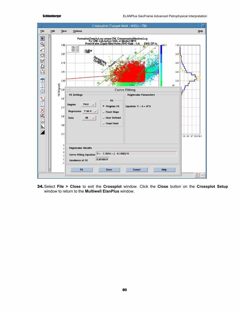
33. Experiment with the other activities on the crossplot window (such as Log Curve Fit).


80

34. Select File > Close to exit the Crossplot window. Click the Close button on the Crossplot Setup window to return to the Multiwell ElanPlus window.


81


Using the multiwell data functioning window, you can apply equation functions on multiple wells.

The purpose of this exercise is how to use Multiwell Data Functioning in ElanPlus Multiwell Mode

Exercise 6.3: Multiwell Data Functioning

1. Continue with the same activity of previous exercise (CrossPlot), if you forget the activity name, just go back to the Process Manager to select the activity you named by using File > Open Activity.




3. Click the Invoke Data Functioning icon to open the Data Functioning window.

4. This function computes values for Volume of Shale, Effective Porosity, and Water Saturation.

5. Select File > Open to load the quickklook_mwelp.func (your instructor will tell you what the directory is) function.


82

6. Use the Parse button to verify the functioning expressions will work, and click OK.

7. Click Bind to verify the input curves are present and click OK. Then click Compute to compute new outputs. Note the zone messages in the main Session Manager Message Area at the bottom of the window.

8. Click List Data to display the List Data window.

9. In the List Data window, highlight all the wells and click Apply to view the outputs. They will appear in the Computation Results section of the Data Functioning window.

10. Finally, click Save Data in the Data Functioning window, followed by Save in the Save Data window, to output the results to the database.

11. Click Close to close the Save Data window. Select File > Close in the Data Functioning window. The saved items will be displayed in the Data Functioning window.

12. Viewing the results:


83

Go to General Data Manager to query for the results computed above, or use Log Curve Data Manager to check from the Database.

Use the template presentation file built from the next exercise (Multiwell cross-section) to display all wells’ computed results.

Question: There is no RW parameter setting for the quicklook_mwelp.func, why this exercise can get right computation?

¿What?


84


The purpose of this exercise is how to use WellCompositePlus Presentation Builder to generate the user customized template file and make multiwell cross section display in ElanPlus Multiwell Mode.

Exercise 6.4 Multiwell Presentation Display

1. Continue with the same activity of previous exercise (CrossPlot), if you forget the activity name, just go back to the Process Manager to select the activity you named by using File > Open Activity.




3. Go back to Process manager and start a new module of WellCompositePlus from the Petrophysics product catalog.

4. Set Data Focus on Well-8B and double-click on WellCompositePlus to open the parameter window.

5. Change the template file to blank.lgp, and click Run to open the main graphics window.


85

6. Click the Presentation Editor icon to open the Presentation Editor main window.

7. In the Presentation Editor main window, click in the text field T1 (beneath the Track Name panel), rename it Depth. Change the Track Width to 0.5.

8. In the Presentation Editor main window, click the Add Track button (beneath the Tracks panel) to add a new track, and name it Shale volume. Change the Track Width to 1.5.

9. In the Presentation Editor main window, click the Add Track button (beneath the Tracks panel) to add a new track and name it Free fluid. Change the Track Width to 1.5.


86

10. In the Presentation Editor main window, click Object Type and select General > Depth/Time Number, then click the Track button and select Depth.

11. Click on the Attribute Editor (AE) icon (scroll to the far right) to change the attributes of depth number.

12. In the Presentation Editor main window, click Object Type and select General > Log Curve, then click the Track button and select Shale volume. Click the blue Add Log Curve button, type in VSH in the Code Selection text field, and click OK to close the window.

13. Click on the Attribute Editor (AE) icon to change the left and right scale to zero, and 1.0.

14. Change the foreground color to blue (you also can change the line thickness and texture).

15. In the Presentation Editor main window, click Object Type and select General > Area Shading, then click the Track button and select Shale volume.

16. Click the blue button Add Area Shading and click the Attribute Editor (AE) icon.

17. In the Area Editor window, modify the filling mode to Fill From To. Click the Boundary 1… button and select Left, and click on Boundary 2… button and select VSH. Select a Shale pattern with a gray background. Click OK.


87

18. In the Presentation Editor main window, click Object Type and select General > Log Curve. Then click the Track button and select Free fluid. Click the blue Add Log Curve button and type in PHIE in the Query by Code text field. Click OK to close the window.

19. Click on the Attribute Editor (AE) icon to change the left and right scale to 0.5 and 0. Change the foreground color to red (you also can change the line thickness and texture).

20. In the Presentation Editor main window, click Object Type and select General > Log Curve, then click

the Track button and select free fluid. Click the blue button Add Log Curve and type in: BVW in the Query By Code text field. Click OK to close the window.

21. Click on the Attribute Editor (AE) icon to change the left and right scale to 0.5 and 0, change the foreground color to red (you also can change the line thickness and texture).

22. In the Presentation Editor main window, click Object Type and select General > Area Shading, then click the Track button and select Free fluid. Click the blue Add Area Shading button and click the

Attribute Editor (AE) icon.


88

23. In the Area Editor window, modify the filling mode as Fill From To (Click on Boundary 1… button and select PHIE, and click on Boundary 2… button and select BVW) and select a Sandstone pattern with a red background. Click OK.

24. Click OK to close the Presentation Editor window. The final display looks like this:


89

25. From WellCompositePlus main window, go to menu File > Save Presentation As to save the graphics as a template file (such as lgp_templates/ quicklook.lgp). Click OK.

26. Go to the Multiwell ElanPlus main window.

27. Select the Cross Section Display icon . In the Setup window, toggle ON Presentation. Click the Presentation button to choose your presentation file (change wa_petroview/*.lgp to lgp_templates/*.lgp and hit <Return> to select quicklook.lgp).

28. Set the Initial Scale to 1/600 and click OK.


90

29. View the Presentation (this is what you calculated from the previous exercise: Multiwell Data Functioning), then File > Close to exit.

Using the similar way, build a presentation file for multiwell ElanPlus results display.

30. Go to WellCompositePlus main window, and start from the blank.lgp.

31. Select the Presentation Editor icon to open the Presentation Editor main window

32. In the Presentation Editor main window, click in the text field T1 (beneath the Track Name panel), rename it Depth, and change the Track Width to 0.5.

33. In the Presentation Editor main window, click the Add Track button beneath the Tracks panel to add a new track. Name it PVP results and change the Track Width to 2.


91

34. In the Presentation Editor main window, click Object Type and select General > Depth/Time Number.

Click the Track button and select Depth. Click the Add Depth/Time Number button, and then click to set up parameters for depth number display.


92

35. In the Presentation Editor main window, click Object Type and select Petrophysics > Elan Volume, then click the Track button and select PVP results. Click the button Add Elan Volume, select PVP FINAL OUTPUTS ELAN_PVP_OUTPUTS, and click OK.

36. Click OK to close the Presentation Editor window.


93

37. From WellCompositePlus main window, go to menu File > Save Presentation As to save the graphics as template file (such as lgp_templates/mwelan.lgp). Click OK.


Multiwell Processing allows you to perform the deterministic computation of reservoir properties for several wells at one time.


94

Perform a dummy run validation before computing

Compute wells by zone

Salinity Initialization logic for Rw/Rwt and Rmf/MST calculations

The purpose of this exercise is how to do multiwell processing by using key well session file in ElanPlus Multiwell Mode.

Exercise 6.5: Multiwell Processing

1. Continue with the same activity of previous exercise (CrossPlot). If you forgot the activity name, just go back to the Process Manager to select the activity you named by using File > Open Activity.

2. If not already selected, move WELL-7B, Well-8B, and Well-9B into the Selected Wells panel in the Multiwell ElanPlus window.



3. Select StrattonB in the Containing Fields panel and click the Attributes button. In the Field Attributes Editor, click the Field Session button and select the Well8-B.elp (the session file you saved from Single Well ElanPlus interpretation) file. Click OK in both windows.

4. In the Session Manager, bring up Edit > Salinity Initialization editor, toggle on the Re-initialize button, and click OK.


95

5. Click the Multiwell Processing Tool icon to open the Validation/Computation window.

6. Press the Bind button to check the data binding well by well. If the required data is not bound correctly, click the Browser button to change the data binding.


96

7. Click Validate to perform a dry or “dummy” run to test that the processing will work. The Process Status window opens.

8. Click Compute and wait until finished. Click Close when finished. (The Save button saves the text of the report to an external file.)

9. Click Close to close the Validation/Computation window.

10. Use the Cross Section Display icon to display the results. Toggle ON the button beside the Presentation File button and click the Presentation File button, and select the file mwelan.lgp you saved in the previous exercise. Click Exit when finished.


97

Saving the session file actually saves the zone sets and well attributes to an ASCII file that can later be loaded to restore the status of the Multiwell session. The data save step saves the zone sets and parameters to the database so that the reservoir summation program can pick up the proper zone boundaries.


98


MultiWell ElanPlus provides a feature to estimate missing logs:

Statistical approach for filling in missing logs with responses from other wells using multi-dimensional histograms

Can be used when estimating missing data is needed for correlation or multi-well field studies

Also useful for estimating core data such as permeability or porosity from multiple input logs.

Exercise 6.6: Missing Log Estimation

Create a Histogram from Several Key Wells

1. From the Multi-Well ElanPlus Session Manager select the StrattonB Field and select Wells 7B, 8B, 9B, 20B. The selected wells should now be listed on the right side of the Session Manager.

2. Select the Log Estimation icon, or click Utilities > Log Estimation.

3. Select Create Histogram as the task (should already be the default).

4. In the field to the right of the Code... button, type GR.

5. Change the Min. to 20 and the Max. to 150. Click Apply.


99

6. Repeat steps 5 and 6 with the following inputs:

Code Min. Max.

NPHI 0.0 0.6

RHOB 1.65 2.65

7. Click View to view the histogram for RHOB.

8. Click Output Histogram... and name a file stratton.his.

9. Click Create... to create the histogram. A histogram is created that will be used to perform the log estimation on another well. A summary will show the number of levels used, cutoff, etc.

10. Close the histogram window.


100

Estimate the GR log in Well-7

1. In the Session Manager, remove Wells 7B, 8B, 9B, 20B from the selection. Select Well 16B.

2. Bring back the Log Estimation window.

3. Change the Task mode (in top left of window) to Estimate Logs.

4. Click Open... and open the “stratton.his” that was created before.

5. An information window pops up to show wells that were used in the creation of the histogram. Click OK to close it.

6. Select NPHI from the Use as Input column, and move it to the Histogram Axis column.

7. Click Estimate... on the bottom to bring up the Axis Selection window.


101

8. Select the NPHI Axis and click OK.

A window showing the progress of estimation appears, followed by a summary of the results. Clicking Detailed will give a depth-by-depth indication of which levels failed to estimate. The “Blank” log problem can be helped by increasing the Nearest Neighbor parameter to one. Click View to check the estimated NPHI.


102

9. Close the Estimate Log window.

View the Estimated Log Results

1. Bring up the Data Manager and highlight Well-16B.

2. From the Query tool, find all arrays in Well-16B with Code = GR.

3. Bring up the WellCompositePlus to show the NPHI comparison. The estimated NPHI will have the extension EST.

In this case, the estimated GR differs from the original GR because the original GR in well 7 was poorly calibrated and is reading too high throughout the well. The estimated GR correctly shows that the GR should be reading lower (verifiable through multi-well crossplots and histograms).

Next step, Create Multiwell lithozone from WellPix; Lump the multiwell properties from ResSum and make 2D distribution (contour/gridding) map for multiwell properties from BaseMapPlus.


103

Chapter 7 Reservoir Property Summation and Mapping (ResSum)

Learning Objectives

After completing this lesson, you will be able to:

Create LithoZones by using WellPix

Perform Reservoir Parameter Summation by using ResSum

Create reservoir summation model

Setup and customize cutoff set for ResSum

View the ResSum result from Data Manager

Visualize ResSum result from BaseMapPlus

Keywords

WellPix, Lithozone, Zone version, Reservoir property summation, Summation model, Cutoff set, Gross, Net, Net reservoir, Net Pay, BaseMapPlus, Porosity, Saturation, Volume of Shale, Permeability


This chapter will describe a workflow for calculating and mapping reservoir properties based on the petrophysical logs and formation markers. This workflow will use the WellPix and ResSum to create lithozones and compute reservoir properties and averages for the zones.

ResSum create sums and averages of log petrophysical properties by zone for one or multiple boreholes. These properties can then be output to a report, and they are saved to the database as part of the zones associated with layers. These properties can then be gridded and mapped in Basemap or CPS-3 products.

For more information on WellPix, ResSum, and Basemap, please refer to the Online Help from the GeoFrame Bookshelf.


104

Exercise 7.2: ResSum Workflow

Data Requirement (Log Curve data and petrophysical analysis data)

Lithozone for specific Zone Version: Created from WellPix Petrophysical analysis data (Porosity, Volume of shale/clay, Water Saturation, Permeability, etc.): Output from petrophysical analysis products (GeoFrame ElanPlus or third party

applications).

Run WellPix to Create a LithoZone

1. From the Application Manager, click the Geology icon to open the Geology Catalog.

2. From the Geology Catalog window, double-click on WellPix to open the WellPix window.

3. From the WellPix window, go to menu File > Template > Open to open the Open Borehole Display Templates dialog box.

4. From the Open Borehole Display Templates dialog box, select WellPix_gr.bdt, and click OK to close the Open Borehole Display Templates dialog box.


105

5. Click All in the Open Template confirmation window.

6. From the WellPix window, go to menu File > Add Boreholes to open the Select Borehole dialog window.

7. From the Select Borehole dialog window, select WELL-7B, WELL-8B, and WELL-9B (use <Ctrl> + MB1 to make multi-selection) and click OK to close the Select Borehole dialog window.

8. Go to View > Depth Scale to open the Depth Scale window.

9. From the Depth Scale window, change Scale to 200, and Major tick to 100. Click OK to close the Depth Scale window.

10. Click Depth… (lower-right corner of the WellPix window) to open the Text Entry window. Type in 6000 and click OK to close the Text Entry window.

11. From the graphic area, click on WELL-7B and go to Edit > Add UDC Template… to open the Open UDC Template dialog box.

12. From the Open UDC Template dialog box, erase the existing text in the Filter text field. Enter directory (your instructor will tell you what it is) /*.lgp and hit Return.

13. Select petro.lgp from the Files panel and click OK to close the window.

14. Click Yes in the UDC Track Propagation confirmation window.

15. Click Zone Version (lower-right corner of the WellPix window) to open the Select Zone Version window.

16. From the Select Zone Version window, click Zone Version Data Manager… to open the Project Zone Version Data Manager window.

17. From the Project Zone Version Data Manager window, enter: stratton_sands_zv in the Name text field.

18. Click OK to create a new Zone Version to store the lithozone which will be created from WellPix, and then Close the Project Zone Version Data Manager window.

19. Click OK to close the Select Zone Version window.


106

20. From WellPix window, select WELL-7B and click the Create Single Litho Zone icon (6th icon from top) to open the Single Litho Zone Interpretation window.


107

21. From the Single Litho Zone Interpretation window, click on Create Layer… button to open the Layer Creation window, type in: stratton_sands in the Layer name text field.

22. Click Upper Surface to open the Feature Boundary window. Select the Stratton Sands from the list panel, and click OK to close the window.

23. Click Lower Surface open the Feature Boundary window. Select the Base Stratton Sands from the list panel, and click OK to close the window.

24. Click Layer Pattern to open the Pattern Selector Panel. Select the sand pattern (column 6, row 3) and click OK to close the window.

25. Click Layer Color to open the Color Selector Panel. Select Gold color, and click on OK to close the window.

26. Click OK to close the Layer Creation window.

27. From the Single Litho Zone Interpretation window, click on Boreholes… to open the Select Boreholes for Single Litho Zone Interpretation window.

28. Select WELL-8B and WELL-9B and click OK to close this window.

29. Toggle ON the Propagate zero-length zones option.

30. Click OK to create the Litho Zone stratton_sands, and close the Single Litho Zone Interpretation window.


108

31. Go to menu File > Exit to close the WellPix window.

Run BaseMapPlus on your secondary screen

32. From the Application Manager window, click the Visualization icon to open the Visualization Catalog window.


109

33. Select Basemap (highlight it) and change the last 0 to 1 in the Display text field, and click OK to run the BaseMapPlus on your secondary screen.

34. Select Create default geological map option, and click OK.

35. Manage the Basemap graphics appearance based on what you have learned about how to use Basemap.

Run ResSum on your Primary screen.

36. From the Geology Catalog window, double-click on ResSum to open the ResSum window.


110

37. From the ResSum window, click on Summation Model… to open the Select a Summation Model window.


111

38. From the Select a Summation Model window, enter the name stratton_sands_model in the Reservoir Summation Model text field and click on Create… to open the Summation Model Definition window.


112

39. From the Summation Model Definition window, click Zone Version… to open the Select Zone Versions window. Select the stratton_sands_zv from the list panel, and click OK to close the Select Zone Versions window.

40. Click Layers… to open the Select Layers window, select the stratton_sands from the list panel. Click OK to close the Select Layers window.

41. Click Boreholes… to open the Select Boreholes window. Select WELL-7B, WELL-8B and WELL-9B and click OK to close the Select Boreholes window.

42. Click OK to close the Summation Model Definition window.

43. From the ResSum window, click Curve Selection… to open the Log Curve Selection dialog box. Click Selected Log Curves to open the Input Curves window. Check to see if Vol. of Shale, Porosity and Water Saturation have been bound with the data from the database, then click OK to close the Input Curves window.


113

44. Click OK to close the Log Curve Selection window.

45. Click Properties… to open the Summation Saved Properties window. Select the properties you wish to calculate, and toggle ON MD and TVD, Zone Property, and Scatter Set options.


114

46. Click OK to close the Summation Saved Properties window.

47. Click Global Cutoff Set… to open the Cutoff Set for Summation Model window.


115

48. From the Cutoff Set for Summation Model window, click New to open the ResSum Text Entry window. Enter the name: cutoff_set1 and click OK to close the window.

49. Highlight cutoff_set1 from the Name list panel and change the Minimum Porosity to 0.15.

50. Toggle OFF Maximum Gamma Ray and Minimum Permeability option.

51. Toggle OFF Curve 1 Code and Curve 2 Code.

52. Click OK to close the Cutoff Set for Summation Model window.

53. In the Property Version text field, erase the existing name and enter: stratton_sands_pv.

54. Highlight all boreholes (WELL-7B, WELL8-B, WELL9-B) in the Boreholes panel in the ResSum window,

and click the Cutoff Set icon to open the Cutoff Set for Boreholes window.


116

55. From the Cutoff Set for Borehole window, select cuttof_set1 and click OK to close it.

56. Highlight all zones in Zones panel of the ResSum window. Click the Cutoff Set icon (first icon) to open the Cutoff Set for Boreholes window. From the Cutoff Set for Borehole window, select cuttof_set1 and click OK to close it.

57. Click Compute to open the Summation Computation window. Click OK to calculate the properties for lithozone.


117

58. Click View to check the results from the Project Zone Data Manager.

59. Go to Results > Print to output the results to a text file or printer.


118

60. Click Setup to specify the properties you wish to post on the Basemap. Drag the property from the Zone Property Selection panel and drop it to the Selected Properties panel. You can select four properties to post in the Basemap window each time. Then click Layers… to select which layer you are going to work with.


119

61. Click Map to post the properties you selected in the Basemap window.

62. In Basemap window, you can grid the properties you posted and map the results.


120

63. In ResSum window, go to menu File > Exit to close the window.

Filename: 08Oct01_ElanPLus_GF4.doc Directory: C:\Documents and Settings\varredon\Desktop Template: C:\Documents and Settings\varredon\Application

Data\Microsoft\Templates\Normal.dot Title: GeoFrame Advanced Petrophysical Interpretation Using

ElanPlus Subject: Author: GeoQuest Keywords: Comments: Creation Date: 10/8/2001 4:56 PM Change Number: 10 Last Saved On: 11/11/2003 11:28 AM Last Saved By: SLB Total Editing Time: 53 Minutes Last Printed On: 11/11/2003 11:29 AM As of Last Complete Printing Number of Pages: 120 Number of Words: 12,314 (approx.) Number of Characters: 70,195 (approx.)