Genomics of Water Use Efficiency Advisory Committee Meeting

Nov 2003

• Comparative mapping– FISH software and related computational methods– Application to tomato fine-mapping

• QTL mapping– experimental design and analysis methodology

• QTL data management– web application

Comparative mapping: computational aspects

• Software needed for two tasks– Identification of homologous chromosomal

segments given two marker maps and information about homology among markers (FISH)

– Prediction of gene content within homologous segments (ongoing work)

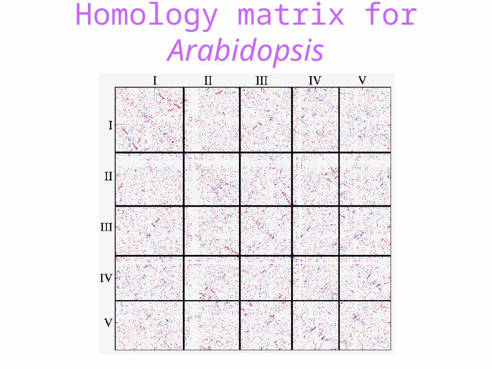
Homology matrix for Arabidopsis

We need to allow for• non-colinearity in marker order• the presence of ‘singleton’ markers

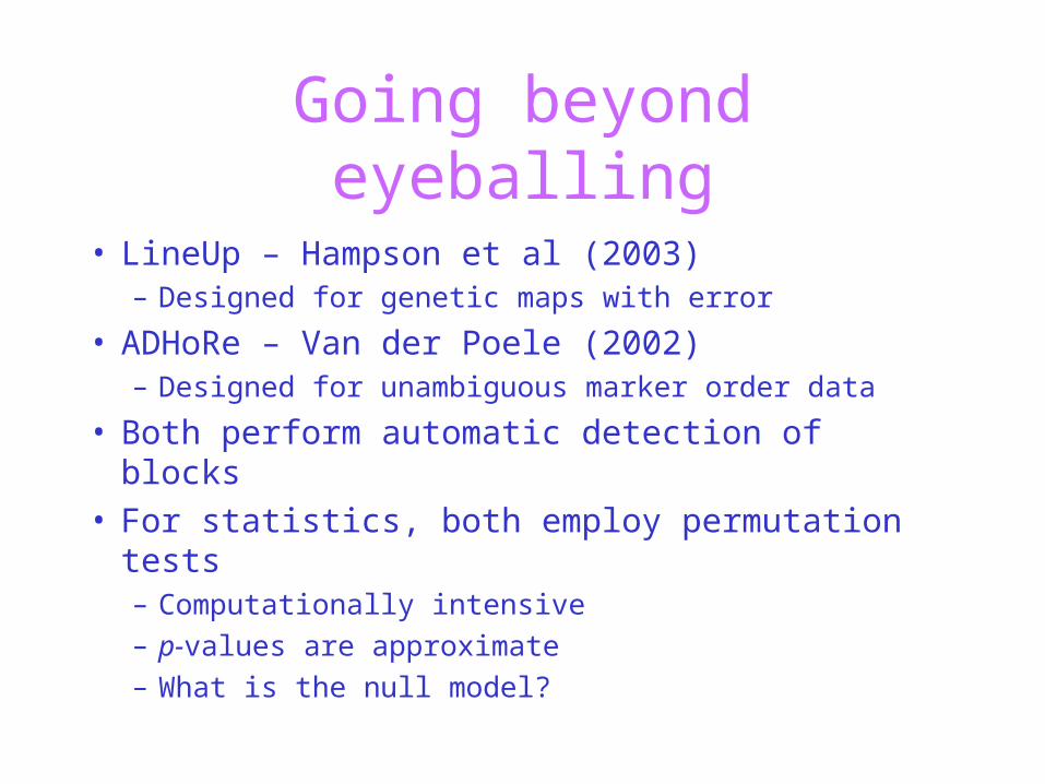
Going beyond eyeballing

• LineUp – Hampson et al (2003)– Designed for genetic maps with error

• ADHoRe – Van der Poele (2002)– Designed for unambiguous marker order data

• Both perform automatic detection of blocks• For statistics, both employ permutation tests

– Computationally intensive– p-values are approximate– What is the null model?

Two contributions

• Local genome alignment

– Dynamic programming approach

• Fast

• Guarantee of optimality

– Can be generalized to multiple alignments

• Statistics

– An explicit null model for marker homology

– Analytic p-values (i.e. no permutation testing)

• Contributors

– Sugata Chakravarty (Masters, UNC Operations Research)

– Peter Calabrese (collaborator, USC)

From homology matrix to graph

• nodes ()– represent dots in the homology

matrix

From homology matrix to graph

• nodes ()– represent dots in the homology

matrix

• edges ()– connect nodes with nearest

neighbors– are unidirectional– have an associated distance– must be shorter than some

threshold

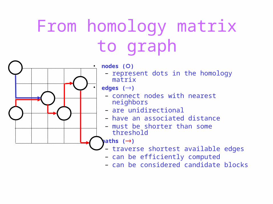
From homology matrix to graph

• nodes ()– represent dots in the homology matrix

• edges ()– connect nodes with nearest neighbors– are unidirectional– have an associated distance– must be shorter than some threshold

• paths ()– traverse shortest available edges– can be efficiently computed– can be considered candidate blocks

Block statistics

• An explicit null model– Within a genome: homologies are due to the duplication of

a feature followed by its insertion into a random position– Between genomes: homologies are due to the above

process plus the transposition of features between randomly chosen positions.

• Number of blocks of a given size is approximately Poisson

• We can calculate – The expected number of blocks of a given size– A conservative matrix-wide p-value

k obs stderr upbound lowbound2 45.8 0.06 47.6 40.13 2.28 0.02 2.39 1.784 0.113 0.003 0.120 0.0795 0.006 0.001 0.006 0.0046 0.0003 0.0002 0.0003 0.0002

How often are blocks of size k observed under the null model compared with expectation (in simulated data)?

FISH v.1.0

• Released in July 2003:– http://www.bio.unc.edu/faculty/vision/lab/FISH– source code – compiled executables– documentation– sample data

• PublicationCalabrese PP, Chakravarty S, Vision TJ  (2003) Fast identification and statistical evaluation of segmental homologies in comparative maps. Bioinformatics 19, i74-i80

Bancroft (2001) TIG 17, 89 after Ku et al (2000) PNAS 97, 9121

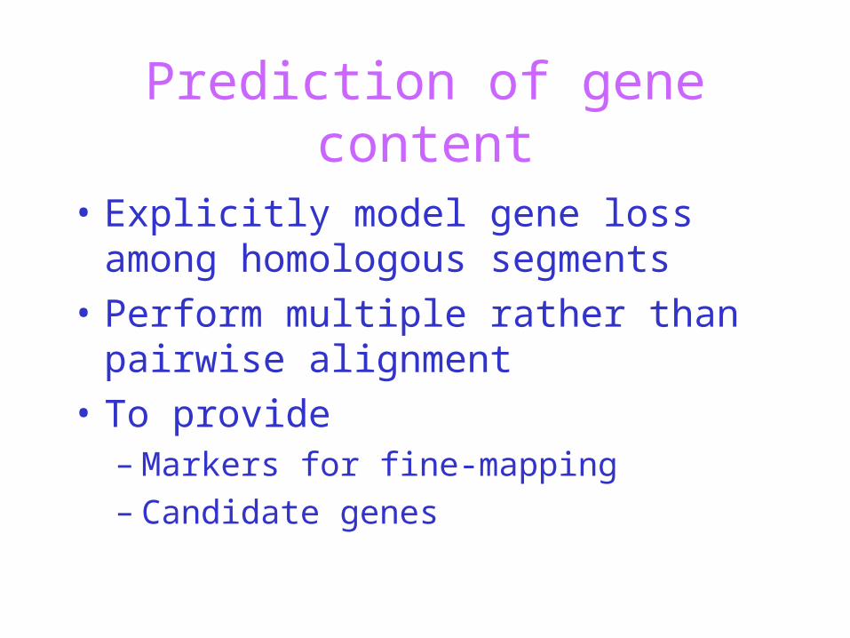
Prediction of gene content

• Explicitly model gene loss among homologous segments

• Perform multiple rather than pairwise alignment

• To provide – Markers for fine-mapping– Candidate genes

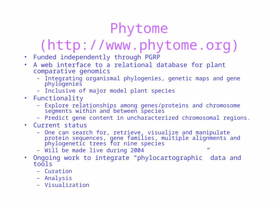
Phytome (http://www.phytome.org)• Funded independently through PGRP• A web interface to a relational database for plant comparative genomics

– Integrating organismal phylogenies, genetic maps and gene phylogenies– Inclusive of major model plant species

• Functionality– Explore relationships among genes/proteins and chromosome segments

within and between species– Predict gene content in uncharacterized chromosomal regions.

• Current status– One can search for, retrieve, visualize and manipulate protein sequences,

gene families, multiple alignments and phylogenetic trees for nine species– Will be made live during 2004

• Ongoing work to integrate “phylocartographic” data and tools– Curation– Analysis– Visualization

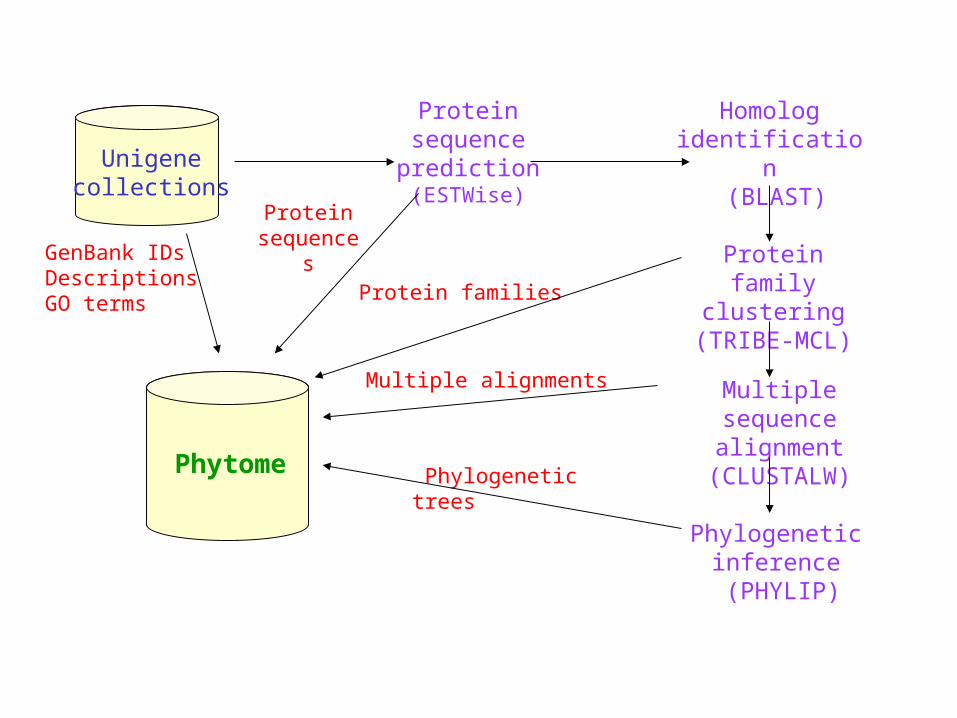
Homolog identification

(BLAST)

Multiple sequence alignment

(CLUSTALW)

Protein sequence prediction(ESTWise)

Protein family clustering

(TRIBE-MCL)

Phylogenetic inference (PHYLIP)

Unigenecollections

GenBank IDsDescriptionsGO terms

Proteinsequences

Protein families

Phylogenetic treesPhytome

Multiple alignments

Comparative mapping in aid of marker development: application

• Complementary to marker development strategy at OK State

• Proposed work (within coming year)– Combine computational predictions and

experimental validation to design PCR-based markers in tomato based on known genes in homologous segments of Arabidopsis

– To be used for fine mapping of QTLs in pennellii (and possible hirsutum).

Comparative map of IL5-4

TG23 TG351 TG60 CHS3 T1584 TG69 CT130 CT145 T0633 TG238 TG597

At1g45160 At1g45474

At1g48490 At1g48520

At2g37840 At2g38050

Atg308720 At3g08940

At4g23650 At4g23710

3

2

20

18

5

Strategyselect Arabidopsis genes in putative regions of synteny

BLAST Arabidopsis genes against tomato EST database

map best match tomato EST in a subset of the IL population

design primers to amplify tomato locus from both parents

no match

maps elsewhere

primers fail

sequence products from both parents to detect polymorphisms

no polymorphism

convert to CAPS or dCAPS markers

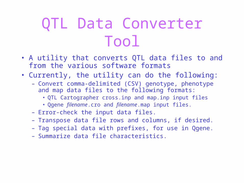
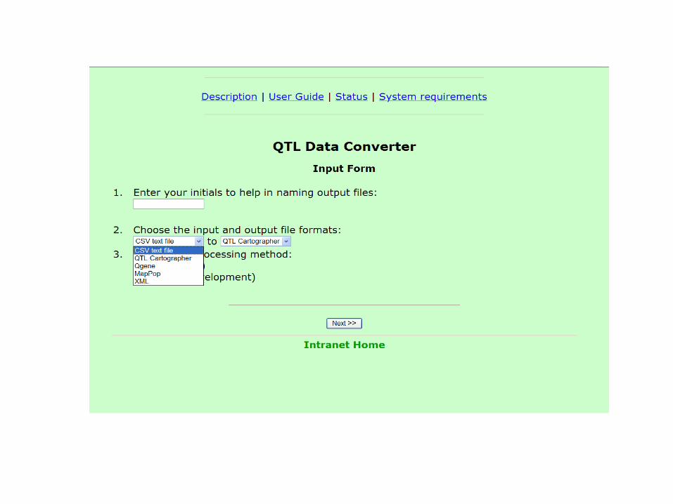
QTL Data Converter Tool

• A utility that converts QTL data files to and from the various software formats

• Currently, the utility can do the following: – Convert comma-delimited (CSV) genotype, phenotype and

map data files to the following formats: • QTL Cartographer cross.inp and map.inp input files • Qgene filename.cro and filename.map input files.

– Error-check the input data files. – Transpose data file rows and columns, if desired. – Tag special data with prefixes, for use in Qgene. – Summarize data file characteristics.

Future plans

• Optimize XML code• Add additional software formats

– MapMaker– MapPop– others as needed (JoinMap, MultiQTL, etc.)

• Release in mid-2004• Advertise availability

– Published note– Mailing list announcements

QTL mapping methodology

• Problem– QTL analysis in mapping populations where individuals have

been selected to optimize marker map resolution.

• Work to date– Effect of selective sampling on crossover distributions– Effect of selective sampling on bias, power, and resolution in

QTL mapping

• Change of plans from proposal– QTL mapping software tailored to selected samples is not

necessary

• Manuscript in preparation for Genetical Research

Bins and map resolutionfull population

optimized sample

X

X

X

random sample

Selective mapping

Genotype framework markers (1/20cM)

base population

Use MapPop to select optimized sample

selected sample

Genotype additional markers (>1/cM)

Use MapPop to locate markers with bin mapping

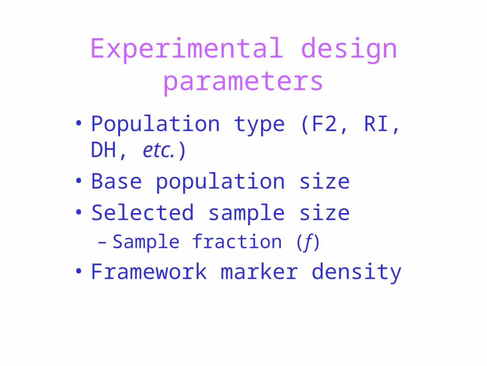
Experimental design parameters

• Population type (F2, RI, DH, etc.)

• Base population size

• Selected sample size– Sample fraction (f)

• Framework marker density

Maize RI population(184 markers, 4140 cM)

Bin Length Whole

N=976

Optimized

N=90

Random

N=90

Maximum 1.8 7.5 12.7

Expected 0.3 1.7 2.6

0

2

4

6

8

10

12

14

16

18

0 5 10 15 20 25 30 35

marker spacing (cM)

Bin

Siz

e (

cM)

MBL perceivedMBL actualEBL perceivedEBL actual

Advantage of optimizing expected (versus maximum) bin size

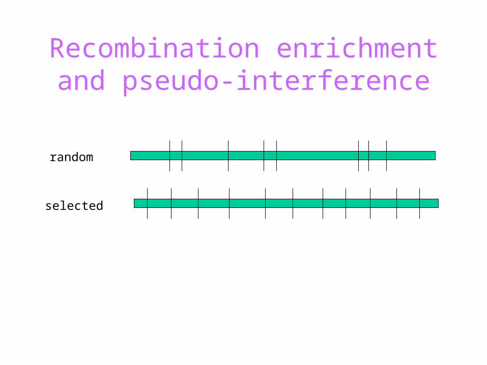
Recombination enrichment and pseudo-interference

random

selected

Recombination enrichment

1

1.5

0.1 0.2 0.3 0.4 0.5 0.6 0.7 0.8 0.9

Sample Fraction

RE

20 cM

10 cM

5 cM

2 cM

1

1.5

2

2.5

0.1 0.2 0.3 0.4 0.5 0.6 0.7 0.8 0.9

Sample Fraction

RE

100 cM500 cM1000 cM2500 cM5000 cM

Fixed map length=1000 cM Fixed marker spacing = 10 cM

RE= # of crossovers in selected sample / # of crossovers in random sample

marker spacing map lgth

Predicting recombination enrichment

Empirical formula: )1(5.01 fL

ARE

L = map length in cM

f = sample fraction

pop A R2

RI 500 0.965

BRI 750 0.976

DH 1200 0.983

Pseudo-interference and map functions

• Translates between the map distance (in cM) and the expected frequency of crossovers between two points

• Haldane map function: no interference• Karlin map function: allows variable interference

• When N>5, rK ~ rH

N

K

mH

N

mr

er

211

2

1

2/)1( ||2

Pseudointerference is very minor

0

10

20

30

40

50

0 0. 2 0. 4 0. 6 0. 8 1

Sampl e Fract i on

N

0

10

20

30

40

50

0 0. 2 0. 4 0. 6 0. 8 1

Sampl e Fract i on

N

0

10

20

30

40

50

0 0. 2 0. 4 0. 6 0. 8 1

Sampl e Fract i on

N

0

10

20

30

40

50

0 0. 2 0. 4 0. 6 0. 8 1Sampl e Fract i on

N

L=1000 cM

L=100 cM L=500 cM

L=2500 cM

5cM 10cM 20cM

Significance of findings

• Since– We can predict RE very accurately and easily from

the experimental design– Pseudointerference is minimal for realistic values

of RE

• We can use standard QTL mapping methods for selected samples once we have multiplied map distances by the RE factor.

• No need for specialized software

Do selected samples have better QTL resolution? A simulation study

• Variables– Population type (RI, BRI, DH)– Map length– Marker spacing (always even)– Sample fraction (optimized for expected bin lgth)– Genetic effects

• Additive ~ Gamma(1,2) • Dominance ~ Beta(1,1) • Pairwise epistasis (when >1 QTL)

• QTL analysis– Marker regression (QTL Cartographer)

QTL detection power

• Reduced in a selected sample in proportion to distance between marker and QTL

• Experimental design– 5 QTL– Map length 1000 cM – Base population 500– Sample fraction 0.2

0

1

2

3

20cM 5cM 1cMMarker spacing

# Q

TL d

etec

ted

selected

random

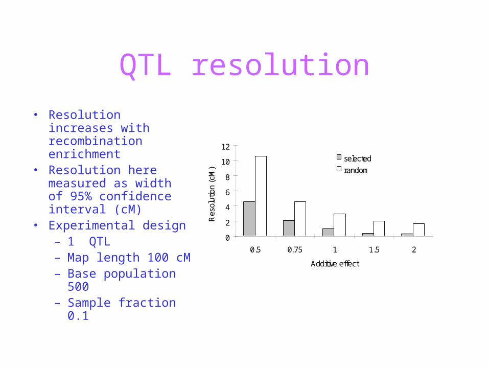
QTL resolution

• Resolution increases with recombination enrichment

• Resolution here measured as width of 95% confidence interval (cM)

• Experimental design– 1 QTL– Map length 100 cM – Base population

500– Sample fraction 0.1

0

2

4

6

8

10

12

0.5 0.75 1 1.5 2

Additive effect

Res

olut

ion

(cM

)

selected

random

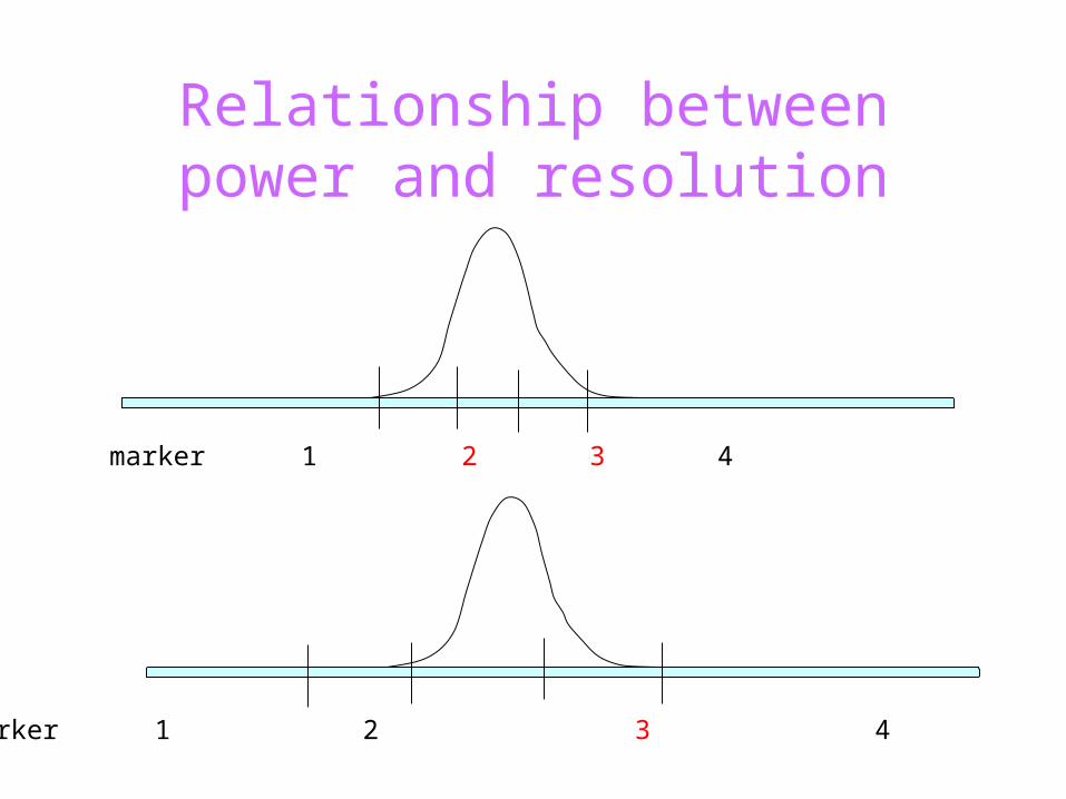
Relationship between power and resolution

marker 1 2 3 4

marker 1 2 3 4

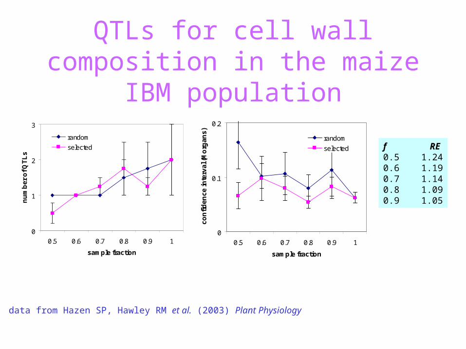
QTLs for cell wall composition in the maize IBM population

data from Hazen SP, Hawley RM et al. (2003) Plant Physiology

0

1

2

3

0.5 0.6 0.7 0.8 0.9 1

sample fraction

nu

mb

er

of

QT

Ls

random

selected

0

0.1

0.2

0.5 0.6 0.7 0.8 0.9 1

sample fraction

co

nfi

de

nc

e in

terv

al (

Mo

rga

ns

)

random

selected f RE0.5 1.240.6 1.190.7 1.140.8 1.090.9 1.05

Summary of findings:QTL mapping methodology

• Selection can result in substantial RE with only minor pseudointerference

• Corrected map distances can be obtained using a simple formula for RE (which will depend on the experimental design)

• Currently available QTL mapping methods are appropriate for analysis of selected samples.

• Selected samples– Have increased QTL mapping resolution (relative to random

ones)– Do not bias estimates of QTL position or effect size