genetics, inheritance & variation -...

Genetics, Inheritance

& Variation

Topic Notes

Additional Support Materials i.e. animations, quizzes,

pictures, worksheets

Principles of Mendelian Inheritance

� Monohybrid test cross

� How genotype controls phenotype

� Sex determination and linkage

� Codominance � Lethal Alleles

� Multiple Alleles

� Dihybrid test cross

� Polygenes

� Epistasis

� Expected ratios, observed ratios and the chi-

squared test

Mendel's Laws (doc)

(Provided by: Ian White)

Mendel Experiment 1 (provided by: Access Excellence)

Mendelian Genetics problem sets and tutorials

(The Biology Project, University of Arizona)

Recessive and Dominant Inheritance

(provided by: Access Excellence)

Sex Linked Inheritance (provided b0y: Access Excellence)

Your Genes, Your Health - Very good

and informative website about genetic diseases and how they are inherited

Meiosis

� Genetic variation in sexual reproduction

� Gene mutation also contributed to variation

Picture comparing Meiosis &

Mitosis (provided by: Access Excellence)

Meiosis tutorial and test yourself (The Biology Project, University of Arizona)

Mitosis & Meiosis interactive

(provided by: Biology in Motion)

Crossing Over and Recombination during Meiosis Picture

(provided by: Access Excellence)

Variation

� Discontinuous variation

� Continuous variation

� Standard deviation and standard error

� Variation gene pool and populations � Hardy-Weinberg equation

Holly Leaf Exercise (doc)

(Provided by: Ian White)

Gene Pool Simulation

(provided by www.Ventrella.com)

Darwin Pond Simulation

(provided by www.Ventrella.com)

Evolution and Variation Revision

(provided by S-cool)

Hardy-Weinberg Problems (provided by: North Harris College)

Basic Science/GeneticsCardiology News and Updates for Physicians www.HeartLinx.com

More Efficient siRNAShortCut RNase III converts dsRNA to potent siRNA in 20 minutes www.neb.com

Proven shRNA silencingLibrary of knock down validated shRNAs and ready to use cell lines. www.RNAx.de

of 19BiologyMad A-Level Biology

10/26/2009http://www.biologymad.com/GeneticsInheritance/geneticsinheritance.htm

Classical Genetics Classical Genetics Classical Genetics Classical Genetics

In module 2 we studied molecular genetics. Here we are concerned with classical genetics, which is the study of inheritance of characteristics at the whole

organism level. It is also known as transmission genetics or Mendelian genetics, since it was pioneered by Gregor Mendel.

Gregor Mendel [back to top]

Mendel (1822-1884) was an Austrian monk at Brno monastery. He was a keen gardener and scientist, and studied at Vienna University, where he learnt

statistics. He investigated inheritance in pea plants and published his results in 1866. They were ignored at the time, but were rediscovered in 1900, and Mendel

is now recognised as the “Father of Genetics”. His experiments succeeded where other had failed because:

� Mendel investigated simple well-defined characteristics (or traits), such as flower colour or seed shape, and he varied one trait at a time. Previous

investigators had tried to study many complex traits, such as human height or intelligence.

� Mendel use an organism whose sexual reproduction he could easily control by carefully pollinating stigmas with pollen using a brush. Peas can also be

self-pollinated, allowing self crosses to be performed. This is not possible with animals.

� Mendel repeated his crosses hundreds of times and applied statistical tests to his results.

� Mendel studied two generations of peas at a time.

A typical experiment looked like this:

Mendel made several conclusions from these experiments:

1. There are no mixed colours (e.g. pink), so this disproved the widely-held blending theories of inheritance that characteristics gradually mixed over time.

2. A characteristic can disappear for a generation, but then reappear the following generation, looking exactly the same. So a characteristic can be present

but hidden.

3. The outward appearance (the phenotype) is not necessarily the same as the inherited factors (the genotype) For example the P1 red plants are not the

same as the F1 red plants.

4. One form of a characteristic can mask the other. The two forms are called dominant and recessive respectively.

5. The F2 ratio is always close to 3:1. Mendel was able to explain this by supposing that each individual has two versions of each inherited factor, one

received from each parent. We’ll look at his logic in a minute.

6. Mendel’s factors are now called genes and the two alternative forms are called alleles. So in the example above we would say that there is a gene for

flower colour and its two alleles are “red” and “white”. One allele comes from each parent, and the two alleles are found on the same position (or locus) on

the homologous chromosomes. With two alleles there are three possible combinations of alleles (or genotypes) and two possible appearances (or

phenotypes):

Genotype Name Phenotype

RR homozygous dominant red

rr homozygous recessive white

Rr, rR heterozygous red



The Monohybrid Cross [back to top]

A simple breeding experiment involving just a single characteristic, like Mendel’s experiment, is called a monohybrid cross. We can now explain Mendel’s

monohybrid cross in detail.

At fertilisation any male gamete can fertilise any female gamete at

random. The possible results of a fertilisation can most easily be worked

out using a Punnett Square as shown in the diagram. Each of the possible

outcomes has an equal chance of happening, so this explains the 3:1 ratio

(phenotypes) observed by Mendel.

This is summarised in Mendel’s First Law, which states that individuals

carry two discrete hereditary factors (alleles) controlling each

characteristic. The two alleles segregate (or separate) during meiosis, so

each gamete carries only one of the two alleles.

The Test Cross

You can see an individual’s phenotype, but you can’t see its genotype. If

an individual shows the recessive trait (white flowers in the above

example) then they must be homozygous recessive as it’s the only

genotype that will give that phenotype. If they show the dominant trait then

they could be homozygous dominant or heterozygous. You can find out

which by performing a test cross with a pure-breeding homozygous

recessive. This gives two possible results:

� If the offspring all show the dominant trait then the parent must be

homozygous dominant.

� If the offspring are a mixture of phenotypes in a 1:1 ratio, then the parent must be heterozygous.

How does Genotype control Phenotype?

Mendel never knew this, but we can explain in detail the relation between an individual’s genes and its appearance. A gene was originally defined as an

inherited factor that controls a characteristic, but we now know that a gene is also a length of DNA that codes for a protein. It is the proteins that actually control

phenotype in their many roles as enzymes, pumps, transporters, motors, hormones, or structural elements. For example the flower colour gene actually codes

for an enzyme that converts a white pigment into a red pigment:

� The dominant allele is the normal (or “wild-type”) form of the gene that codes for functioning enzyme, which therefore makes red-coloured flowers.

� The recessive allele is a mutation of the gene. This mutated gene codes for non-functional enzyme, so the red pigment can’t be made, and the flower

remains white. Almost any mutation in a gene will result in an inactive gene product (usually an enzyme), since there are far more ways of making an

inactive protein than a working one.

Sometimes the gene actually codes for a protein apparently unrelated to the phenotype. For example the gene for seed shape in peas (round or wrinkled)

actually codes for an enzyme that synthesises starch! The functional enzyme makes lots of starch and the seeds are full and rounded, while the non-functional

enzyme makes less starch so the seeds wrinkle up.



This table shows why the allele that codes for a functional protein is usually dominant over an allele that codes for a non-function protein. In a heterozygous cell,

some functional protein will be made, and this is usually enough to have the desired effect. In particular, enzyme reactions are not usually limited by the amount

of enzyme, so a smaller amount will have little effect.

Sex Determination [back to top]

In module 2 we saw that sex is determined by the sex chromosomes (X and Y). Since these are non-homologous they are called heterosomes, while the other

22 pairs are called autosomes. In humans the sex chromosomes are homologous in females (XX) and non-homologous in males (XY), though in other species

it is the other way round. The inheritance of the X and Y chromosomes can be demonstrated using a monohybrid cross:

This shows that there will always be a 1:1 ratio of males to females. Note that female gametes (eggs) always contain a single X chromosome, while the male

gametes (sperm) can contain a single X or a single Y chromosome. Sex is therefore determined solely by the sperm. There are techniques for separating X and

Y sperm, and this is used for planned sex determination in farm animals using IVF.

Sex Linkage

The X and Y chromosomes don’t just determine sex, but also contain many other genes that have nothing to do with sex determination. The Y chromosome is

very small and seems to contain very few genes, but the X chromosome is large and contains thousands of genes for important products such as rhodopsin (a

protein in the membrane of a photoreceptor cell in the retina of the eye, basically a light absorbing pigment), blood clotting proteins and muscle proteins.

Females have two copies of each gene on the X chromosome (i.e. they’re diploid), but males only have one copy of each gene on the X chromosome (i.e.

they’re haploid). This means that the inheritance of these genes is different for males and females, so they are called sex linked characteristics.

The first example of sex linked genes discovered was eye colour in Drosophila fruit flies. Red eyes (R) are dominant to white eyes (r) and when a red-eyed

female is crossed with a white-eyed male, the offspring all have red eyes, as expected for a dominant characteristic (left cross below). However, when the

opposite cross was done (a white-eye male with a red-eyed female) all the male offspring had white eyes (right cross below). This surprising result was not

expected for a simple dominant characteristic, but it could be explained if the gene for eye colour was located on the X chromosome. Note that in these crosses

the alleles are written in the form XR (red eyes) and Xr (white eyes) to show that they are on the X chromosome.

Genotype Gene product Phenotype

homozygous dominant (RR) all functional enzyme red

homozygous recessive (rr) no functional enzyme white

heterozygous (Rr) some functional enzyme red



Males always inherit their X chromosome from their mothers, and always pass on their X chromosome to their daughters.

Another well-known example of a sex-linked characteristic is colour blindness in humans. 8% of males are colour blind, but only 0.7% of females. The genes for

green-sensitive and red-sensitive rhodopsin are on the X chromosome, and mutations in either of these lead to colour blindness. The diagram below shows two

crosses involving colour blindness, using the symbols XR for the dominant allele (normal rhodopsin, normal vision) and Xr for the recessive allele (non-functional

rhodopsin, colour blind vision).

Other examples of sex linkage include haemophilia, premature balding and muscular dystrophy.

Codominance [back to top]

In most situations (and all of Mendel’s experiments) one allele is completely dominant over the other, so there are just two phenotypes. But in some cases there

are three phenotypes, because neither allele is dominant over the other, so the heterozygous genotype has its own phenotype. This situation is called

codominance or incomplete dominance. Since there is no dominance we can no longer use capital and small letters to indicate the alleles, so a more formal

system is used. The gene is represented by a letter, and the different alleles by superscripts to the gene letter.

A good example of codominance is flower colour in snapdragon (Antirrhinum) plants. The flower colour gene C has two alleles: CR (red) and CW (white). The

three genotypes and their phenotypes are:

In this case the enzyme is probably less active, so a smaller amount of enzyme will make significantly less product, and this leads to the third phenotype. The

monohybrid cross looks like this:

Genotype Gene product Phenotype

homozygous RR all functional enzyme red

homozygous WW no functional enzyme white

heterozygous (RW) some functional enzyme pink



Note that codominance is not an example of “blending inheritance” since the original phenotypes reappear in the second generation. The genotypes are not

blended and they still obey Mendel’s law of segregation. It is only the phenotype that appears to blend in the heterozygotes.

Another example of codominance is sickle cell haemoglobin in humans. The gene for haemoglobin Hb has two codominant alleles: HbA (the normal gene) and

HbS (the mutated gene). There are three phenotypes:

Other examples of codominance include coat colour in cattle (red/white/roan), and coat colour in cats (black/orange/tortoiseshell).

Lethal Alleles [back to top]

An unusual effect of codominance is found in Manx cats, which have no tails. If two Manx cats are crossed the litter has ratio of 2 Manx kittens to 1 normal

(long-tailed) kitten. The explanation for this unexpected ratio is explained in this genetic diagram:

HbAHbA Normal. All haemoglobin is normal, with normal red blood cells.

HbAHbS Sickle cell trait. 50% of the haemoglobin in every red blood cell is normal, and 50% is

abnormal. The red blood cells are slightly distorted, but can carry oxygen, so this condition

is viable. However these red blood cells cannot support the malaria parasite, so this

phenotype confers immunity to malaria.

HbSHbS Sickle cell anaemia. All haemoglobin is abnormal, and molecules stick together to form

chains, distorting the red blood cells into sickle shapes. These sickle red blood cells are

destroyed by the spleen, so this phenotype is fatal.



The gene S actually controls the development of the embryo cat’s spine. It has two codominant alleles: SN (normal spine) and SA (abnormal, short spine). The

three phenotypes are:

Many human genes also have lethal alleles, because many genes are so essential for life that a mutation in these genes is fatal. If the lethal allele is expressed

early in embryo development then the fertilised egg may not develop enough to start a pregnancy, or the embryo may miscarry. If the lethal allele is expressed

later in life, then we call it a genetic disease, such as muscular dystrophy or cystic fibrosis.

Multiple Alleles [back to top]

An individual has two copies of each gene, so can only have two alleles of any gene, but there can be more than two alleles of a gene in a population. An

example of this is blood group in humans. The red blood cell antigen is coded for by the gene I (for isohaemaglutinogen), which has three alleles IA, IB and IO.

(They are written this way to show that they are alleles of the same gene.) IA and IB are codominant, while IO is recessive. The possible genotypes and

phenotypes are:

The cross below shows how all four blood groups can arise from a cross between a group A and a group B parent.

Other examples of multiple alleles are: eye colour in fruit flies, with over 100 alleles; human leukocyte antigen (HLA) genes, with 47 known alleles.

SNSN Normal. Normal spine, long tail

SNSA Manx Cat. Last few vertebrae absent, so no tail.

SASA Lethal. Spine doesn’t develop, so this genotype is fatal early in development. The embryo

doesn’t develop and is absorbed by the mother, so there is no evidence for its existence.

Phenotype

(blood group) Genotypes

antigens on red blood cells

plasma antibodies

A IAIA, IAIO A anti-B

B IBIB, IBIO B anti-A

AB IAIB A and B none

O IOIO none anti-A and anti-B



Multiple Genes

So far we have looked at the inheritance of a single gene controlling a single characteristic. This simplification allows us to understand the basic rules of

heredity, but inheritance is normally much more complicated than that. We’ll now turn to the inheritance of characteristics involving two genes. This gets more

complicated, partly because there are now two genes to consider, but also because the two genes can interact with each other. We’ll look at three situations:

� 2 independent genes, controlling 2 characteristics (the dihybrid cross).

� 2 independent genes controlling 1 characteristic (polygenes)

� 2 interacting genes controlling 1 characteristic (epistasis)

The Dihybrid Cross

Mendel also studied the inheritance of two different characteristics at a time in pea plants, so we’ll look at one of his dihybrid crosses. The two traits are seed

shape and seed colour. Round seeds (R) are dominant to wrinkled seeds (r), and yellow seeds (Y) are dominant to green seeds (y). With these two genes there

are 4 possible phenotypes:

Mendel’s dihybrid cross looked like this:

All 4 possible phenotypes are produced, but always in the ratio 9:3:3:1. Mendel was able to explain this ratio if the factors (genes) that control the two

characteristics are inherited independently; in other words one gene does not affect the other. This is summarised in Mendel’s second law (or the law of

independent assortment), what states that alleles of different genes are inherited independently.

We can now explain the dihybrid cross in detail.

Genotypes Phenotype

RRYY, RRYy, RrYY, RrYy round yellow

RRyy, Rryy round green

rrYY, rrYy wrinkled yellow

rryy wrinkled green



The gametes have one allele of each gene, and that allele can end up with either allele of the other gene. This gives 4 different gametes for the second

generation, and 16 possible genotype outcomes.

Dihybrid Test Cross [back to top]

There are 4 genotypes that all give the same round yellow phenotype. Just like we saw with the monohybrid cross, these four genotypes can be distinguished

by crossing with a double recessive phenotype. This gives 4 different results:

Polygenes [back to top]

Sometimes two genes at different loci (i.e. separate genes) can combine to affect one single characteristic. An example of this is coat colour in Siamese cats.

One gene controls the colour of the pigment, and black hair (B) is dominant to brown hair (b). The other gene controls the dilution of the pigment in the hairs,

with dense pigment (D) being dominant to dilute pigment (d). This gives 4 possible phenotypes:

Original genotype Result of test cross

RRYY all round yellow

RRYy 1 round yellow : 1 round green

RrYY 1 round yellow : 1 wrinkled yellow

RrYy 1 round yellow : 1 round green: 1 wrinkled yellow: 1 wrinkled green

Genotypes Phenotype F2 ratio

BBDD, BBDd, BbDD, BbDd “seal” (black dense) 9

BBdd, Bbdd “blue” (black dilute) 3

bbDD, bbDd “chocolate” (brown dense) 3



The alleles are inherited in exactly the same way as in the dihybrid cross above, so the same 9:3:3:1 ratio in the F2 generation is produced. The only difference

is that here, we are looking at a single characteristic, but with a more complicated phenotype ratio than that found in a monohybrid cross.

A more complex example of a polygenic character is skin colour in humans. There are 5 main categories of skin colour (phenotypes) controlled by two genes at

different loci. The amount of skin pigment (melanin) is proportional to the number of dominant alleles of either gene:

Some other examples of polygenic characteristics are: eye colour, hair colour, and height. The important point about a polygenic character is that it can have a

number of different phenotypes, and almost any phenotypic ratio

Epistasis [back to top]

In epistasis, two genes control a single character, but one of the genes can mask the effect of the other gene. A gene that can mask the effect of another gene

is called an epistatic gene (from the Greek meaning “to stand on”). This is a little bit like dominant and recessive alleles, but epistasis applies to two genes at

different loci. Epistasis reduces the number of different phenotypes for the character, so instead of having 4 phenotypes for 2 genes, there will be 3 or 2. We’ll

look at three examples of epistasis.

1. Dependent genes. In mice one gene controls the production of coat pigment, and black pigment (B) is dominant to no pigment (b). Another gene controls

the dilution of the pigment in the hairs, with dense pigment (D) being dominant to dilute pigment (d). This is very much like the Siamese cat example above, but

with one important difference: the pigment gene (B) is epistatic over the dilution gene (D) because the recessive allele of the pigment gene is a mutation that

produces no pigment at all, so there is nothing for the dilution gene to affect. This gives 3 possible phenotypes:

2. Enzymes in a pathway. In a certain variety of sweet pea there are two flower colours (white and purple), but the F2 ratio is 9:7. This is explained if the

production of the purple pigment is controlled by two enzymes in a pathway, coded by genes at different loci.

Gene P is epistatic over gene Q because the recessive allele of gene P is a mutation that produces inactive enzyme, so there is no compound B for enzyme Q

to react with. This gives just two possible phenotypes:

3. Duplicate Genes. This occurs when genes at two different loci make enzyme that can catalyse the same reaction (this can happen by gene duplication). In

this case the coloured pigment is always made unless both genes are present as homozygous recessive (ppqq), so the F2 ratio is 15:1.

bbdd “lilac” (brown dilute) 1

Phenotype

(skin colour)

Genotypes No. of dominant

alleles F2 ratio

Black AABB 4 1

Dark AaBB, AABb 3 4

Medium AAbb, AaBb, aaBB 2 6

Light Aabb, aaBb 1 4

White (albino) aabb 0 1


BBDD, BBDd, BbDD, BbDd Black (black dense) 9

BBdd, Bbdd Brown (black dilute) 3

bbDD, bbDd, bbdd White (no pigment) 4


PPQQ, PPQq, PpQQ, PpQq Purple 9

PPqq, Ppqq, ppQQ, ppQq, ppqq White 7



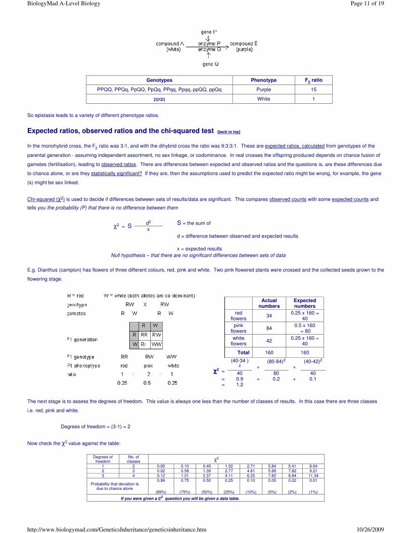
So epistasis leads to a variety of different phenotype ratios.

Expected ratios, observed ratios and the chi-squared test [back to top]

In the monohybrid cross, the F2 ratio was 3:1, and with the dihybrid cross the ratio was 9:3:3:1. These are expected ratios, calculated from genotypes of the

parental generation - assuming independent assortment, no sex linkage, or codominance. In real crosses the offspring produced depends on chance fusion of

gametes (fertilisation), leading to observed ratios. There are differences between expected and observed ratios and the questions is, are these differences due

to chance alone, or are they statistically significant? If they are, then the assumptions used to predict the expected ratio might be wrong, for example, the gene

(s) might be sex linked.

Chi-squared (χ2) is used to decide if differences between sets of results/data are significant. This compares observed counts with some expected counts and

tells you the probability (P) that there is no difference between them

E.g. Dianthus (campion) has flowers of three different colours, red, pink and white. Two pink flowered plants were crossed and the collected seeds grown to the

flowering stage.

The next stage is to assess the degrees of freedom. This value is always one less than the number of classes of results. In this case there are three classes

i.e. red, pink and white.

Degrees of freedom = (3-1) = 2

Now check the χ2 value against the table:


PPQQ, PPQq, PpQQ, PpQq, PPqq, Ppqq, ppQQ, ppQq Purple 15

ppqq White 1

χ2 = S d2 x

S = the sum of

d = difference between observed and expected results

x = expected results Null hypothesis – that there are no significant differences between sets of data

Actual numbers

Expected numbers

red flowers

34 0.25 x 160 =

40

pink flowers

84 0.5 x 160

= 80

white flowers

42 0.25 x 160 =

40

Total 160 160

χχχχ2 =

(40-34 )2 +

(80-84)2 +

(40-42)2

40 80 40 = 0.9 + 0.2 + 0.1 = 1.2

Degrees of freedom

No. of classes χ2

1 2 0.00 0.10 0.45 1.32 2.71 3.84 5.41 6.64 2 3 0.02 0.58 1.39 2.77 4.61 5.99 7.82 9.21 3 4 0.12 1.21 2.37 4.11 6.25 7.82 9.84 11.34

Probability that deviation is due to chance alone

0.99

(99%)

0.75

(75%)

0.50

(50%)

0.25

(25%)

0.10

(10%)

0.05

(5%)

0.02

(2%)

0.01

(1%) If you were given a c2 question you will be given a data table.



� Go to the 2 degrees freedom line

� Find the nearest figures to 1.2, which comes between 75% and 50% columns

� A χ2 value of 1.2 shows that it is at least 50% probable that the result is by chance alone.

� For a significant difference the value should fall between 1-5% columns. The difference of this result against the expected is not significant. Therefore

the null hypothesis is accepted.

Meiosis

[back to top]

Meiosis is the special form of cell division used to produce gametes. It has two important functions:

� To form haploid cells with half the normal chromosome number

� To re-arrange the chromosomes with a novel combination of genes (genetic recombination)

Meiosis comprises two successive divisions, without DNA replication in between. The second division is a bit like mitosis, but the first division is different in

many important respects. The details are shown in this diagram for a hypothetical cell with 2 pairs of homologous chromosomes (n=2):

First Division Second Division

Interphase I

� chromatin not visible

� DNA & proteins replicated

Interphase II

� Short

� no DNA replication

� chromosomes remain

visible.

Prophase I

� chromosomes visible

� homologous chromosomes

join together to form a

bivalent

� chromatids cross over

(chiasmata – see below)

Prophase II

� centrioles replicate and

move to new poles.

Metaphase I

� bivalents line up on equator

Metaphase II

� chromosomes line up on

equator.

Anaphase I

� chromosomes separate

(not chromatids-

centromere doesn’t split)

Anaphase II

� centromeres split

� chromatids separate.

Telophase I

� nuclei form

� cell divides

Telophase II

� 4 haploid cells, each with

2 chromatids

� cells often stay together to



Genetic Variation in Sexual Reproduction [back to top]

As mentioned in module 2, the whole point of meiosis and sex is to introduce genetic variation, which allows species to adapt to their environment and so to

evolve. There are three sources of genetic variation in sexual reproduction:

� Independent assortment in meiosis

� Crossing over in meiosis

� Random fertilisation

We’ll look at each of these in turn.

1. Independent Assortment

This happens at metaphase I in meiosis, when the bivalents line up on the equator. Each bivalent is made up of two homologous chromosomes, which originally

came from two different parents (they’re often called maternal and paternal chromosomes). Since they can line up in any orientation on the equator, the

maternal and paternal versions of the different chromosomes can be mixed up in the final gametes.

In this simple example with 2 homologous chromosomes (n=2) there are 4 possible different gametes (22). In humans with n=23 there are over 8 million

possible different gametes (223). Although this is an impressively large number, there is a limit to the mixing in that genes on the same chromosome must

always stay together. This limitation is solved by crossing over.

2. Crossing Over

This happens at prophase I in meiosis, when the bivalents first form. While the two homologous chromosomes are joined in a bivalent, bits of one chromosome

are swapped (crossed over) with the corresponding bits of the other chromosome.

The points at which the chromosomes actually cross over are called chiasmata (singular chiasma), and they involve large, multi-enzyme complexes that cut and

join the DNA. There is always at least one chiasma in a bivalent, but there are usually many, and it is the chiasmata that actually hold the bivalent together. The

chiasmata can be seen under the microscope and they can give the bivalents some strange shapes at prophase I. There are always equal amounts crossed

over, so the chromosomes stay the same length. Ultimately, crossing over means that maternal and paternal alleles can be mixed, even though they are on the

same chromosome i.e. chiasmata result in different allele combinations.

3. Random Fertilisation

This takes place when two gametes fuse to form a zygote. Each gamete has a unique combination of genes, and any of the numerous male gametes can

� cells have 2 chromosomes,

not 4 chromatids.

form a tetrad.



fertilise any of the numerous female gametes. So every zygote is unique.

These three kinds of genetic recombination explain Mendel’s laws of genetics (described above).

Gene Mutation also contributes to Variation [back to top]

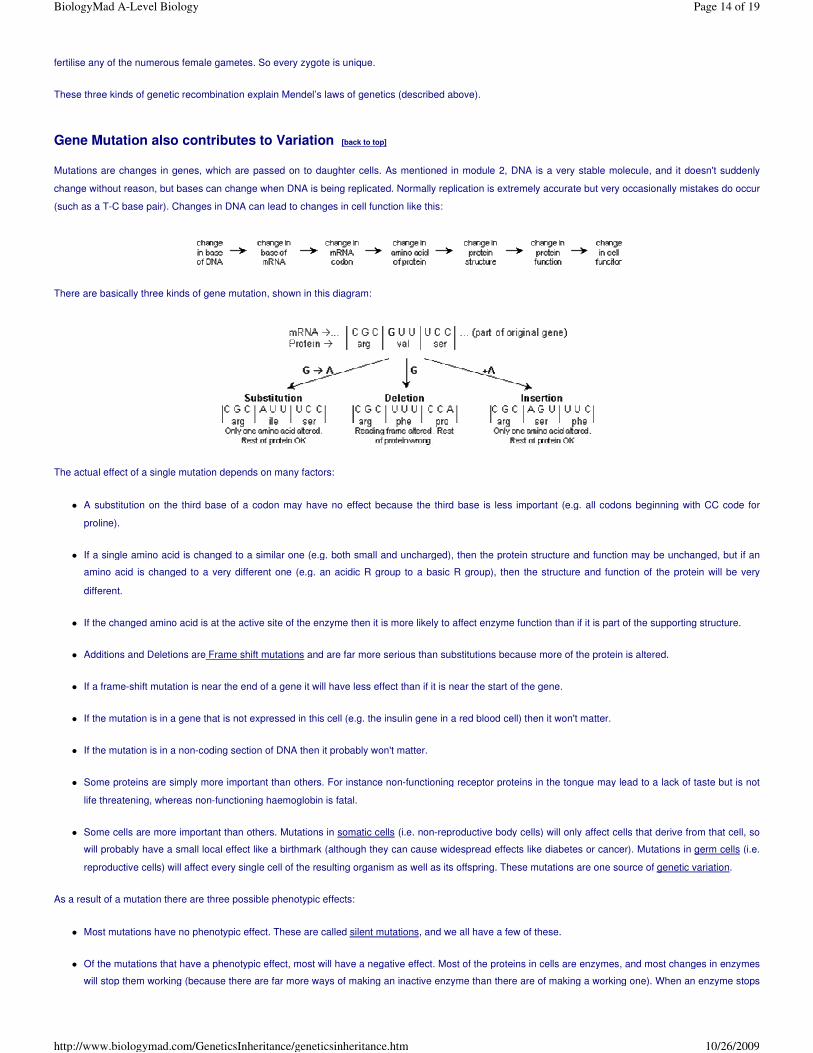
Mutations are changes in genes, which are passed on to daughter cells. As mentioned in module 2, DNA is a very stable molecule, and it doesn't suddenly

change without reason, but bases can change when DNA is being replicated. Normally replication is extremely accurate but very occasionally mistakes do occur

(such as a T-C base pair). Changes in DNA can lead to changes in cell function like this:

There are basically three kinds of gene mutation, shown in this diagram:

The actual effect of a single mutation depends on many factors:

� A substitution on the third base of a codon may have no effect because the third base is less important (e.g. all codons beginning with CC code for

proline).

� If a single amino acid is changed to a similar one (e.g. both small and uncharged), then the protein structure and function may be unchanged, but if an

amino acid is changed to a very different one (e.g. an acidic R group to a basic R group), then the structure and function of the protein will be very

different.

� If the changed amino acid is at the active site of the enzyme then it is more likely to affect enzyme function than if it is part of the supporting structure.

� Additions and Deletions are Frame shift mutations and are far more serious than substitutions because more of the protein is altered.

� If a frame-shift mutation is near the end of a gene it will have less effect than if it is near the start of the gene.

� If the mutation is in a gene that is not expressed in this cell (e.g. the insulin gene in a red blood cell) then it won't matter.

� If the mutation is in a non-coding section of DNA then it probably won't matter.

� Some proteins are simply more important than others. For instance non-functioning receptor proteins in the tongue may lead to a lack of taste but is not

life threatening, whereas non-functioning haemoglobin is fatal.

� Some cells are more important than others. Mutations in somatic cells (i.e. non-reproductive body cells) will only affect cells that derive from that cell, so

will probably have a small local effect like a birthmark (although they can cause widespread effects like diabetes or cancer). Mutations in germ cells (i.e.

reproductive cells) will affect every single cell of the resulting organism as well as its offspring. These mutations are one source of genetic variation.

As a result of a mutation there are three possible phenotypic effects:

� Most mutations have no phenotypic effect. These are called silent mutations, and we all have a few of these.

� Of the mutations that have a phenotypic effect, most will have a negative effect. Most of the proteins in cells are enzymes, and most changes in enzymes

will stop them working (because there are far more ways of making an inactive enzyme than there are of making a working one). When an enzyme stops



working, a metabolic block can occur, when a reaction in cell doesn't happen, so the cell's function is changed. An example of this is the genetic disease

phenylketonuria (PKU), caused by a mutation in the gene for the enzyme phenylalanine hydroxylase. This causes a metabolic block in the pathway

involving the amino acid phenylalanine, which builds up, causing mental retardation.

� Very rarely a mutation can have a beneficial phenotypic effect, such as making an enzyme work faster, or a structural protein stronger, or a receptor

protein more sensitive. Although rare beneficial mutations are important as they drive evolution.

The kinds of mutations discussed so far are called point or gene mutations because they affect specific points within a gene. There are other kinds of mutation

that can affect many genes at once or even whole chromosomes. These chromosome mutations can arise due to mistakes in cell division. A well-known

example is Down syndrome (trisonomy 21) where there are three copies of chromosome 21 instead of the normal two.

Mutation Rates and Mutagens

Mutations are normally very rare, which is why members of a species all look alike and can interbreed. However the rate of mutations is increased by chemicals

or by radiation. These are called mutagenic agents or mutagens, and include:

� High energy ionising radiation such as x-rays, ultraviolet rays, α, β, or γ rays from radioactive sources. These ionise the bases so that they don't form the

correct base pairs.

� Intercalating chemicals such as mustard gas (used in World War 1), which bind to DNA separating the two strands.

� Chemicals that react with the DNA bases such as benzene, nitrous acid, and tar in cigarette smoke.

� Viruses. Some viruses can change the base sequence in DNA causing genetic disease and cancer.

During the Earth's early history there were far more of these mutagens than there are now, so the mutation rate would have been much higher than now,

leading to a greater diversity of life. Some of these mutagens are used today in research, to kill microbes or in warfare. They are often carcinogens since a

common result of a mutation is cancer.

Variation [back to top]

Variation means the differences in characteristics (phenotype) within a species. There are many causes of variation as this chart shows:

Variation consists of differences between species as well as differences within the same species. Each individual is influenced by the environment, so this is

another source of variation.

genotype + environment = phenotype

The alleles that are expressed in the phenotype can only perform their function efficiently if they have a supply of suitable substances and have appropriate

conditions. Any study of variation inevitably involves the collection of large quantities of data.

When collecting the data there is a need for random sampling. This involves choosing a sample ‘at random’ from a population. This means that every member

of the population has the same chance of being chosen, and that the choices are independent of one another. In choosing a random sample some things are

very important:



� the selection criteria must not correspond to what you are studying i.e. not introduce any systematic bias.

� you must try to maintain independence of the sample points

� you muse be careful in making inference: the population might not be what you wish it were

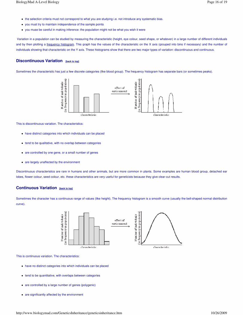
Variation in a population can be studied by measuring the characteristic (height, eye colour, seed shape, or whatever) in a large number of different individuals

and by then plotting a frequency histogram. This graph has the values of the characteristic on the X axis (grouped into bins if necessary) and the number of

individuals showing that characteristic on the Y axis. These histograms show that there are two major types of variation: discontinuous and continuous.

Discontinuous Variation [back to top]

Sometimes the characteristic has just a few discrete categories (like blood group). The frequency histogram has separate bars (or sometimes peaks).

This is discontinuous variation. The characteristics:

� have distinct categories into which individuals can be placed

� tend to be qualitative, with no overlap between categories

� are controlled by one gene, or a small number of genes

� are largely unaffected by the environment

Discontinuous characteristics are rare in humans and other animals, but are more common in plants. Some examples are human blood group, detached ear

lobes, flower colour, seed colour, etc. these characteristics are very useful for geneticists because they give clear-cut results.

Continuous Variation [back to top]

Sometimes the character has a continuous range of values (like height). The frequency histogram is a smooth curve (usually the bell-shaped normal distribution

curve).

This is continuous variation. The characteristics:

� have no distinct categories into which individuals can be placed

� tend to be quantitative, with overlaps between categories

� are controlled by a large number of genes (polygenic)

� are significantly affected by the environment



Continuous characteristics are very common in humans and other animals. Some examples are height, hair colour, heart rate, muscle efficiency, intelligence,

growth rate, rate of photosynthesis, etc.

Characteristics that show continuous variation are controlled not by one, but by the combined effect of a number of genes, called polygenes. Therefore any

character, which results from the interaction of many genes, is called a polygenic character. The random assortment of genes during prophase I of meiosis

ensures that individuals possess a range of genes from any polygenic complex.

Sometimes you can see the effect of both variations. For example the histogram of height of humans can be bimodal

(i.e. it’s got two peaks). This is because the two sexes (a discontinuous characteristic) each have their own normal

distribution of height (a continuous characteristic).

Standard Deviation and Standard Error [back to top]

Standard deviation is a measure of the spread of results at either side of the mean (average).

� These sets of data have the same mean (average).

� The data shows a normal distribution about the mean value – there is a bell-shaped and even distribution of values above and below the mean.

� The diagram on the left shows a smaller standard deviation, indicating there is less variation between individuals for the character mentioned.

� The diagram on the right shows a greater standard deviation, indicating there is greater variation.

The standard error is the standard deviation of the mean.

� If individuals in a number of samples are measured, then each sample will have its own mean.

� These means will usually be slightly different from each other – reflecting chance differences in samples – giving a range of values for sample means.

� Standard error is a measure of how much the value of a sample mean is likely to vary.

� The greater the standard error, the greater the variation of the mean.

Variation , Gene Pool and Populations [back to top]

It is at the population level that evolution occurs. A population is a group of individuals of the same species in a given area whose members can interbreed.

Because the individuals of a population can interbreed, they share a common group of genes known as the gene pool. Each gene pool contains all the alleles

for all the traits of all the population. For evolution to occur in real populations, some of the gene frequencies must change with time. The gene frequency of an

allele is the number of times an allele for a particular trait occurs compared to the total number of alleles for that trait.

Hardy – Weinberg Equation [back to top]

G. H. Hardy, an English mathematician, and W.R. Weinberg, a German physician, independently worked out the effects of random mating in successsive

generations on the frequencies of alleles in a population. This is important for biologists because it is the basis of hypothetical stability from which real change

Gene frequency = the number of a specific type of allele the total number of alleles in the gene pool



can be measured

An important way of discovering why real populations change with time is to construct a model of a population that does not change. This is just what Hardy and

Weinberg did. Their principle describes a hypothetical situation in which there is no change in the gene pool (frequencies of alleles), hence no evolution.

Consider a population whose gene pool contains the alleles A and a. Hardy and Weinberg assigned the letter p to the frequency of the dominant allele A and

the letter q to the frequency of the recessive allele a. Since the sum of all the alleles must equal 100%, then p + q = 1. They then reasoned that all the random

possible combinations of the members of a population would equal (p+q)2 or p2+ 2pq + q2.

The Hardy-Weinberg equation p2 + 2pq + q2 = 1

The frequencies of A and a will remain unchanged generation after generation if the following conditions are met:

1. Large population. The population must be large to minimize random sampling errors.

2. Random mating. There is no mating preference. For example an AA male does not prefer an aa female.

3. No mutation. The alleles must not change.

4. No migration. Exchange of genes between the population and another population must not occur.

5. No natural selection. Natural selection must not favour any particular individual.

The results show that Hardy-Weinberg Equilibrium was not maintained. The migration of swimmers (genes) into the pool (population) resulted in a change in the

population's gene frequencies. If the migrations were to stop and the other agents of evolution (i.e., mutation, natural selection and non-random mating) did not

occur, then the population would maintain the new gene frequencies generation after generation. It is important to note that a fifth factor affecting gene

frequencies is population size. The larger a population is the number of changes that occur by chance alone becomes insignificant. In the analogy above, a

small population was deliberately used to simplify the explanation.

[back to top]

Let’s look at an analogy to help demonstrate Hardy-

Weinberg Equilibrium. Imagine a ‘swimming’ pool

of genes as shown in Figure 1.

Find: Frequencies of A and a. and the genotypic

frequencies of AA, Aa and aa.

Solution:

f(A) = 12/30 = 0.4 = 40%

f(a) = 18/30 = 0.6 = 60%

then, p + q = 0.4 + 0.6 = 1

and p2 + 2pq + q2 = AA + Aa + aa

= .24 + .48 + .30 = 1

As long as the conditions of Hardy-Weinberg are met, the population can increase in size and the gene

frequencies of A and a will remain the same. Thus, the gene pool does not change.

Now, suppose more 'swimmers' dive in as shown in

Figure 2. What will the gene and genotypic

frequencies be?

Solution:

f(A) = 12/34 = .35 = 35 %

f(a) = 22/34 = .65 = 65%

f(AA) = .12, f(Aa) = .23 and f (aa) = .42



Last updated 20/06/2004



genetics, inheritance & variation -...

Documents