Generative and Discriminative Models in NLP:

A Survey

Kristina ToutanovaComputer Science Department

Stanford University

Motivation

Many problems in natural language processing are disambiguation problems word senses

jaguar – a big cat, a car, name of a Java package

line - phone, queue, in mathematics, air line, etc. part-of-speech tags (noun, verb, proper noun,

etc.)

? ? ?Joy makes progress every day .

NN

VBDT NN

NN

NNP

VBZ

NNS

Motivation

Parsing – choosing preferred phrase structure trees for sentences, corresponding to likely semantics

Possible approaches to disambiguation Encode knowledge about the problem, define rules,

hand-engineer grammars and patterns (requires much effort, not always possible to have categorical answers)

Treat the problem as a classification task and learn classifiers from labeled training data

VBD

“Mary”

NNP

S

“I”

VPNP

“saw”

PPIN NNP

“with”“the”“telescope”

?

Overview

General ML perspective Examples The case of Part-of-Speech Tagging The case of Syntactic Parsing Conclusions

The Classification Problem

Given a training set of iid samples T={(X1,Y1) … (Xn,Yn)} of input and class variables from an unknown distribution D(X,Y), estimate a function that predicts the class from the input variables

The goal is to come up with a hypothesis with minimum expected loss (usually 0-1 loss)

Under 0-1 loss the hypothesis with minimum expected loss is the Bayes optimal classifier

YX

XhYYXDherr,

))(ˆ(),()ˆ(

)|(maxarg)( XYDXhY

)(ˆ Xh

)(ˆ Xh

Approaches to Solving Classification Problems - I

1. Generative. Try to estimate the probability distribution of the data D(X,Y)

specify a parametric model family choose parameters by maximum

likelihood on training data

estimate conditional probabilities by Bayes rule

classify new instances to the most probable class Y according to

)(/),()|( ˆˆˆ XPYXPXYP

)|(ˆ XYP

}:),({ YXP

),()|(1

ii

n

i

YXPTL

Approaches to Solving Classification Problems - I

2. Discriminative. Try to estimate the conditional distribution D(Y|X) from data.

specify a parametric model family estimate parameters by maximum

conditional likelihood of training data classify new instances to the most

probable class Y according to

3. Discriminative. Distribution-free. Try to estimate directly from data so that its expected loss will be minimized

}:)|({ XYP

)|(ˆ XYP

)|(),|(

1ii

n

i

XYPXTCL

)(ˆ Xh

Axes for comparison of different approaches

Asymptotic accuracy Accuracy for limited training data Speed of convergence to the best

hypothesis Complexity of training Modeling ease

Generative-Discriminative Pairs

Definition: If a generative and discriminative parametric model family can represent the same set of conditional probability distributions they are a generative-discriminative pair

Example: Naïve Bayes and Logistic RegressionY

X2X1

},...,2,1{ KY }1,0{, 21 XX

Ki

NB iYXPiYXPiYP

iYXPiYXPiYPXXiYP

...121

2121 )|()|()(

)|()|()(),|(

Kiiii

iiiLR XX

XXXXiYP

...102211

0221121 )exp(

)exp(),|(

)|( XYP

Comparison of Naïve Bayes and Logistic Regression

The NB assumption that features are independent given the class is not made by logistic regression

The logistic regression model is more general because it allows a larger class of probability distributions for the features given classes

)exp()exp()(

),()|,(

)|()|()|,(

02211

...102211

2121

2121

iii

Kiiii

LR

NB

XXXXiYP

XXPiYXXP

iYXPiYXPiYXXP

Example: Traffic Lights

Lights Working

Lights Broken

P(g,r,w) = 3/7 P(r,g,w) = 3/7 P(r,r,b) = 1/7

Working?

NS EW

Model assumptions false! JL and CL estimates differ…

JL: P(w) = 6/7 CL: (w) = P(r|w)= ½ (r|w) = ½P(r|b) = 1 (r|b) = 1

NB Model

Reality

P~

P~

P~

P~

Joint Traffic LightsLights Working

Lights Broken

3/14 3/14 3/14 3/14

2/14

Conditional likelihood of working is 1

Conditional likelihood of working is > ½! Incorrectly assigned!

Accuracy: 6/7

0 00

Conditional Traffic LightsLights Working

Lights Broken

1-

Conditional likelihood of working is still 1

Now correctly assigned to broken.

/4 /4 /4 /4

Accuracy: 7/7CL perfect (1)JL low (to 0)

0 0 0

Comparison of Naïve Bayes and Logistic Regression

Naïve Bayes Logistic Regression

Accuracy +

Convergence +

Training Speed +

Model assumptions

independence of features given class

Linear log-odds

Advantages Faster convergence, uses information in P(X), faster training

More robust and accurate because fewer assumptions

Disadvantages Large bias if the independence assumptions are very wrong

Harder parameter estimation problem, ignores information in P(X)

))|,(

)|,(log(

21

21

jYXXP

iYXXP

15

20

25

30

35

40

45

50LRNB

Some Experimental Comparisons

err

or

training data size

0

10

20

30

40

50

60

5 1000 2000 3000 4000

LRNB

training data sizeerr

or

Ng & Jordan 2002

(15 datasets from UCI ML)

Klein & Manning 2002(WSD line and hard data)

Part-of-Speech Tagging

POS tagging is determining the part of speech of every word in a sentence.

? ? ? Joy makes progress every day .Sequence classification problem with 45 classes (Penn

Treebank). Accuracies are high 97%! Some argue it can’t go much higher

Existing approaches: rule-based (hand-crafted, TBL) generative (HMM) discriminative (maxent, memory-based, decision tree, neural

network, linear models(boosting,perceptron) )

NNNN

VBDT

NN

NNP

VBZ

NNS

Part-of-Speech TaggingUseful Features

The complete solution of the problem requires full syntactic and semantic understanding of sentences

In most cases information about surrounding words/tags is strong disambiguator

“The long fenestration was tiring . “ Useful features

tags of previous/following words P(NN|JJ)=.45;P(VBP|JJ)=0.0005

identity of word being tagged/surrounding words suffix/prefix for unknown words, hyphenation,

capitalization longer distance features others we haven’t figured out yet

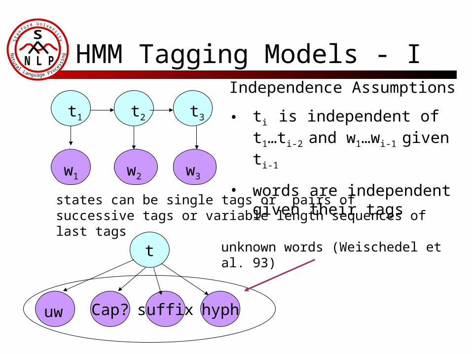
HMM Tagging Models - I

t1 t2 t3

w1 w2 w3

states can be single tags or pairs of successive tags or variable length sequences of last tags

t

uw

Independence Assumptions

• ti is independent of t1…ti-2

and w1…wi-1 given ti-1

• words are independent given their tags

Cap? suffix hyph

unknown words (Weischedel et al. 93)

HMM Tagging Models - Brants 2000

Highly competitive with other state-of-the art models

Trigram HMM with smoothed transition probabilities

Capitalization feature becomes part of the state – each tag state is split into two e.g. NN <NN,cap>,<NN,not cap>

Suffix features for unknown words

)(ˆ/)|(~

)(ˆ

)|)(|()|(

tagPsuffixtagPsuffixP

suffixwtagsuffixPtagwP

)(ˆ...)|(ˆ)|(ˆ)|(~

121 tagPsuffixtagPsuffixtagPsuffixtagP nnnn

t

suffixn

suffixn-1 suffix2 suffix1

CMM Tagging Models

t1 t2 t3

w1 w2 w3

Independence Assumptions

• ti is independent of t1…ti-2

and w1…wi-1 given ti-1

• ti is independent of all following observations

• no independence assumptions on the observation sequence•Dependence of current tag on previous and future

observations can be added; overlapping features of the observation can be taken as predictors

MEMM Tagging Models -II

Ratnaparkhi (1996) local distributions are estimated using maximum

entropy models used previous two tags, current word, previous two

words, next two words suffix, prefix, hyphenation, and capitalization

features for unknown words

Model Overall Accuracy

Unknown Words

HMM (Brants 2000) 96.7 85.5

MEMM(Ratn 1996) 96.63 85.56

MEMM(T&M 2000) 96.86 86.91

HMM vs CMM – I

Model Accuracy

95.5%

94.4%

95.3%

tj

wj+1wj

tj+1

tj

wj+1wj

tj+1

tj

wj+1wj

tj+1

Johnson (2001)

HMM vs CMM - II

The per-state conditioning of the CMM has been observed to exhibit label bias (Bottou, Lafferty) and observation bias (Klein & Manning )

Klein & Manning (2002)HMM CMM CMM+

91.23 89.22 90.44

Unobserving words with unambiguous tags improved performance significantly

t1 t2 t3

w1 w2 w3

t1 t2 t3

w1 w2 w3

Conditional Random Fields (Lafferty et al 2001)

Models that are globally conditioned on the observation sequence; define distribution P(Y|X) of tag sequence given word sequence

No independence assumptions about the observations; no need to model their distribution

The labels can depend on past and future observations

Avoids the independence assumption of CMMs that labels are independent of future observations and thus the label and observation bias problems

The parameter estimation problem is much harder

CRF - II

HMM and this chain CRF form a generative-discriminative pair

Independence assumptions : a tag is independent of all other tags in the sequence given its neighbors and the word sequence

t1 t2 t3

w1 w2 w3

nn

jjjj

jjjj

Tttwt

n

jtt

wt

n

jtt

nn wwttP

... 1

111

1

1

1

))(exp(

))(exp(

)...|...(

CRF-Experimental Results

Model Accuracy Unknown Word Accuracy

HMM 94.31% 54.01%

CMM (MEMM) 93.63% 45.39%

CRF 94.45% 51.95%

CMM+ (MEMM+)

95.19% 73.01%

CRF+ 95.73% 76.24%

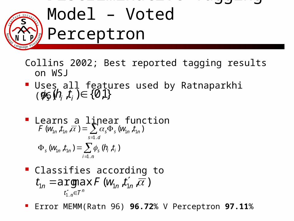
Discriminative Tagging Model – Voted Perceptron

Collins 2002; Best reported tagging results on WSJ

Uses all features used by Ratnaparkhi (96)

Learns a linear function

Classifies according to

Error MEMM(Ratn 96) 96.72% V Perceptron 97.11%

}1,0{),( iis th

),(),(

),(),,(

..111

11..1

11

iini

snns

nnds

ssnn

thtw

twtwF

),,(maxarg 111..1

nnTt

n twFtn

n

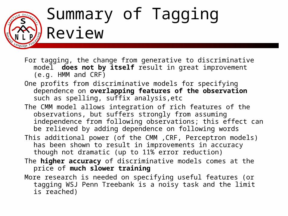
Summary of Tagging Review

For tagging, the change from generative to discriminative model does not by itself result in great improvement (e.g. HMM and CRF)

One profits from discriminative models for specifying dependence on overlapping features of the observation such as spelling, suffix analysis,etc

The CMM model allows integration of rich features of the observations, but suffers strongly from assuming independence from following observations; this effect can be relieved by adding dependence on following words

This additional power (of the CMM ,CRF, Perceptron models) has been shown to result in improvements in accuracy though not dramatic (up to 11% error reduction)

The higher accuracy of discriminative models comes at the price of much slower training

More research is needed on specifying useful features (or tagging WSJ Penn Treebank is a noisy task and the limit is reached)

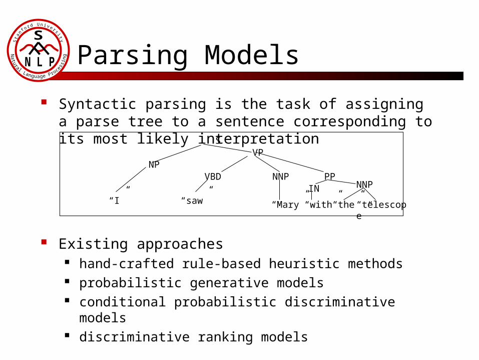
Syntactic parsing is the task of assigning a parse tree to a sentence corresponding to its most likely interpretation

Existing approaches hand-crafted rule-based heuristic methods probabilistic generative models conditional probabilistic discriminative models discriminative ranking models

Parsing Models

VBD

“Mary”

NNP

“I”

VPNP

“saw”

PPIN NNP

“with”“the”“telescope”

S

Generative Parsing Models Generative models based on PCFG grammars learned

from corpora are still among the best performing (Collins 97,Charniak 97,00) 88% -89% labeled precision/recall

The generative models learn a distribution P(X,Y) on <sentence, parse tree> pairs:

and select a single most likely parse for a sentence X

based on:

Easy to train using RFE for maximum likelihood These models have the advantage of being usable as

language models (Chelba&Jelinek 00, Charniak 00)

),(maxarg)(yield:

YXPYXYY

best

))(history|)(expansion(),()(

nnPYXPYnodesn

Generative History-Based Model – Collins 97

TOP

S(bought)

NP(week) NP-C(Marks) VP(bought)

VBD(bought)

NP-C(Brooks)

“bought”

NNP(Brooks)

“Brooks”

NNP(Marks)

“Marks”

JJ(Last)

“week”“Last”

NN(week)

Accuracy <= 100 words

88.1% LP 87.5% LR

Discriminative models

Shift-reduce parser Ratnaparkhi (98) Learns a distribution P(T|S) of parse trees given

sentences using the sequence of actions of a shift-reduce parser

Uses a maximum entropy model to learn conditional distribution of parse action given history

Suffers from independence assumptions that actions are independent of future observations as CMM

Higher parameter estimation cost to learn local maximum entropy models

Lower but still good accuracy 86% - 87% labeled precision/recall

)...|()|( 111

SaaaPSTP i

n

ii

Discriminative Models – Distribution Free Re-ranking

Represent sentence-parse tree pairs by a feature vector F(X,Y)

Learn a linear ranking model with parameters using the boosting loss

Model LP LR

Collins 99(Generative)

88.3% 88.1%

Collins 00(BoostLoss)

89.9% 89.6%

13% error reduction

Still very close in accuracy to generative model (Charniak 00)

Comparison of Generative-Discriminative Pairs

Johnson (2001) have compared simple PCFG trained to maximize L(T,S) and L(T|S)

A Simple PCFG has parameters

Models:

Results:

)),,((maxarg..1

iini

STPLogMLE

},1),|({...1

iAAPimjijijiij

)),|((maxarg..1

iini

STPLogMCLE

Model LPrecision

LRecall

MLE 0.815 0.789

MCLE 0.817 0.794

Weighted CFGs for Unification-Based Grammars - I

Unification-based grammars (UBG) are often defined using a context-free base and a set of path equationsS[number X] -> NP[number X] VP[number X]NP[number X] -> N [number X]VP[number X] ->V[number X]N[number sg]-> dog ; N[number pl] ->dogs;

V[number sg] ->barks ; V[number pl] ->bark; A PCFG grammar can be defined using the

context-free backbone CFGUBG(S-> NP, VP) The UBG generates “dogs bark” and “dog

barks”. The CFGUBG generates “dogs bark” ,“dog barks”, “dog bark”, and “dogs barks” .

Weighted CFGs for Unification-Based Grammars - II

A Simple PCFG for CFGUBG has parameters from the set

It defines a joint distribution P(T,S) and a conditional

distributions of trees given sentences

A conditional weighted CFG defines only a conditional probability; the conditional probability of any tree T outside the UBG is 0

},1),|({...1

iAAPimjijijiij

)(, )(

)()|(

STYieldCFGT TnodesnExpA

TnodesnExpA

PCFG

UBG

nn

nn

STP

)(, )(

)()|(

STYieldUBGT TnodesnExpA

TnodesnExpA

CWCFG

nn

nn

UBGSTP

Weighted CFGs for Unification-based grammars - III

47,7

66,3

76,7

48,7

79,381,8

45

50

55

60

65

70

75

80

85

HMMTagger

PCFG-S PCFG-A

Generative

Conditional log-linear

The conditional weighted CFGs perform consistently better than their generative counterparts

Negative information is extremely helpful here; knowing that the conditional probability of trees outside the UBG is zero plus conditional training amounts to 38% error reduction for the simple PCFG model

Accu

racy

Summary of Parsing Results

The single small study comparing a parsing generative-discriminative pair for PCFG parsing showed a small (insignificant) advantage for the discriminative model; the added computational cost is probably not worth it

The best performing statistical parsers are still generative(Charniak 00, Collins 99) or use a generative model as a preprocessing stage(Collins 00, Collins 2002) (part of which has to do with computational complexity)

Discriminative models allow more complex representations such as the all subtrees representation (Collins 2002) or other overlapping features (Collins 00) and this has led to up to 13% improvement over a generative model

Discriminative training seems promising for parse selection tasks for UBG, where the number of possible analyses is not enormous

Conclusions

For the current sizes of training data available for NLP tasks such as tagging and parsing, discriminative training has not by itself yielded large gains in accuracy

The flexibility of including non-independent features of the observations in discriminative models has resulted in improved part-of-speech tagging models (for some tasks it might not justify the added computational complexity)

For parsing, discriminative training has shown improvements when used for re-ranking or when using negative information (UBG)

if you come up with a feature that is very hard to incorporate in a generative models and seems extremely useful, see if a discriminative approach will be computationally feasible !