GENERATION OF VOLUME MESHES BY EXTRUSION FROM SURFACE MESHES OF ARBITRARY TOPOLOGY

David S. Thompson1, Satish Chalasani2, Bharat K. Soni3

Mississippi State University, Mississippi State, MS., U.S.A 1dst@erc.msstate.edu, 2satish@erc.msstate.edu, 3bsoni@erc.msstate.edu

ABSTRACT

An algorithm to generate volume meshes by extrusion from surface meshes of arbitrary topology is presented. The algorithm utilizes a three-step, advancing layer scheme to extrude a smooth volume mesh starting from an initial surface mesh. First, a locally orthogonal reference mesh is algebraically generated for the layer. The reference mesh is then smoothed using a locally three-dimensional Poisson-type mesh generation equation that is generalized to smooth extruded meshes of arbitrary surface topology. By using the Poisson equation, control functions developed for elliptic grid generation may be employed to improve mesh quality. The Poisson smoother is modified in concave regions to enhance the robustness of the advancing layer scheme. Several preliminary examples are included to demonstrate the efficacy of the approach. Keywords: mesh generation, hybrid meshes, elliptic smoothing, Winslow smoothing

1. INTRODUCTION

Mesh generation operates fundamentally by distributing points throughout the volume of a physical region, as well as on its bounding surfaces. Connection of the points forms the mesh and subdivides the physical region into a filling set of discrete volume elements. Structured grids [1]-[6] and unstructured meshes [7]-[9] have been used successfully to solve a wide range of problems in computational mechanics. Each of these mesh types has advantages and disadvantages that have been well documented in the literature. It seems apparent that no single mesh type can simultaneously address the conflicting requirements of solution accuracy, computational efficiency, and automation of the grid generation process. In an attempt to reconcile these conflicting requirements, an approach combining elements of both structured grids and unstructured meshes, the so-called hybrid grid method [10]-[13], has been developed. Hybrid grids are attractive because of their flexibility with respect to automation as well as feature resolution through the use of anisotropic elements. Additionally, hybrid topologies require significantly fewer elements than unstructured meshes to achieve the same

resolution [10]. In a typical hybrid grid, prismatic or hexahedral cells are used in regions of the domain near boundaries dominated by large gradients in the field variables. These near-body cells are generated by extrusion of the surface mesh into the domain. Once the mesh is extruded sufficiently far into the domain, tetrahedra are employed to fill the remaining voids. If an extruded surface of the mesh contains quadrilaterals, a pyramidal transition layer must be generated at the interface between the quadrilaterals and the tetrahedra. During the near-body mesh generation phase of a typical hybrid grid generation algorithm, the surface normals are first smoothed followed by an extrusion. Laplcian smoothing is then applied to the resulting layer [12]. An alternative approach for generating prismatic meshes using hyperbolic PDEs seems to have been first suggested by Steger [14]. A similar technique was employed by Matsuno [15] in a recent paper. In [15], the hyperbolic grid generation equations were used to extrude a prismatic volume mesh starting from a triangular surface mesh. An “upwind-biased” finite-difference scheme was used to discretize the hyperbolic mesh generation equations. It should be noted that the example meshes shown in [15] did not exhibit the smoothness normally associated with PDE-based grid generation approaches.

With the exception of [10], most hybrid grid generation technologies require that the surface discretization be uniformly of the same type. Using triangles may result in an excessively large number of faces being needed to adequately discretize the surface, thereby affecting solution efficiency. If structured quadrilaterals are used, a manual surface decomposition must be performed that requires significant effort. Clearly, there are advantages to using a surface mesh whose topology is appropriate for the region being discretized. A related approach was utilized by Wey who employed a mixed hexahedral/prismatic, near-body grid generation algorithm for generating Chimera grids [16]. The mesh generation techniques mentioned above are related to the so-called “sweep methods” used to generate all-hexahedral meshes for two-and-one-half dimensional geometries [17]-[19]. In a sweep method, a set of topologically identical surfaces is generated between the source and target meshes along a defined sweep axis. However, the topology of the source mesh is arbitrary. The bounding loops of these swept surfaces or, alternatively, a prescribed surface linking the source and target meshes is also specified. The interior point placement is then determined via an algorithm designed to provide a quality mesh. However, the sweeping algorithms do not appear appropriate for source meshes with significant convex or concave regions interior to the mesh not captured by their respective bounding loops. In this paper we describe an extension of the extrusion technique described in [20] and [21] for surface meshes of arbitrary topology. Here, we focus on the algorithm used to generate near-body meshes appropriate for viscous flow simulations. We have employed a modified form of Knupp's weighted-Winslow smoother [22] for a surface mesh of arbitrary topology. Knupp's smoother, termed a weighted-Poisson smoother, is essentially a Poisson mesh generation equation with the control functions designed to transmit information about the relative spacing of points from a source mesh to a copied or morphed mesh. However, the weighted Poisson smoother of [22] is strictly a surface smoother and, as such, is not appropriate for smoothing a surface with significant convex/concave regions in its interior unless some method is employed to constrain the resulting out of surface deformations. Here we employ a parabolic method to generate the mesh in layers using a modified form of the surface smoother to smooth a locally orthogonal reference mesh [4]-[6]. The surface smoother is modified by including a three-dimensional term, which, in conjunction with the reference mesh, effectively constrains the deformation of the interior of the surface mesh. It should be noted that the smoothing is performed in each layer as the mesh is generated and is not applied a posteriori. Therefore, this smoothing is best described as locally three-dimensional. An additional benefit of this locally three-dimensional smoothing is that the mesh remains nearly orthogonal except in strongly convex or concave regions. We first provide an overview of the algorithm. Next we provide a discussion of the application of a locally three-dimensional Poisson smoothing to extruded, unstructured meshes. The specifics of the algorithm are then presented

including a discussion of a modification of the Poisson smoother in regions where the smoothed mesh is concave. We then present several preliminary meshes to illustrate the efficacy of the method.

2. ALGORITHM OVERVIEW

In the near-body mesh generation algorithm described below, the mesh is extruded in layers starting from the initial surface mesh. Generation of the mesh within each layer is accomplished using a modification of the parabolic mesh generation strategies [4]-[6] developed for structured meshes and can be described as a three-step process: • A three-level, locally orthogonal, reference mesh is

generated by extrusion of the initial surface mesh in the direction of the local surface normal following a prescribed distance distribution. The reference mesh consists of the initial data surface for the layer and two extruded levels.

• The intermediate level of the reference mesh is

iteratively smoothed using the Poisson smoothing equation. The third level of the mesh is adjusted after each iteration to reflect the changes in the surface normals of the second level as it is smoothed.

• The third level of the reference mesh is then discarded

and the second level is used as the initial data surface for the next layer and the process is repeated.

Since the smoothing is applied to each layer as the mesh is being generated, it can best be characterized as locally three-dimensional. By design, the resulting smoothed mesh still exhibits many of the characteristics of the reference mesh. In this respect, it is fair to characterize the mesh as nearly orthogonal. The greatest deviation from orthogonality occurs where the smoother has done the most work.

3. APPLICATION OF POISSON SMOOTHING TO EXTRUDED, UNSTRUCTURED MESHES

As stated previously, Laplacian smoothing is typically used to smooth the near-body extruded layers in hybrid mesh generation [12]. It is well known that Winslow smoothing [23] is superior to Laplacian smoothing because Winslow smoothing, being based on harmonic analysis, is more resistant to mesh folding than Laplacian smoothing. However, Winslow smoothing provides no mechanism for propagating the relative spacing of the points on the initial surface mesh into the domain. On the other hand, the use of Poisson smoothing equations, while not as resistant to mesh folding as Winslow smoothing, permits the use of control functions to influence the spacing of points on the extruded surfaces [23]. Of course, the basic assumption here is that the initial surface mesh has desirable characteristics. In structured grid generation [1], a global transformation of the form

)z,y,x(

)z,y,x(

)z,y,x(

ζ=ζη=ηξ=ξ

(Eq. 1)

is typically employed. The inverse transform

),,(zz

),,(yy

),,(xx

ζηξ=ζηξ=ζηξ=

(Eq. 2)

is also assumed to exist. Assuming that ζ is the marching (extrusion) direction and that ζ lines are orthogonal to the extruded ζ=constant surface, the Poisson equation commonly used for structured grid generation becomes

0

)(g

ggg

g

gg2

)(g

gg)(

g

gg

2

2122211

23312

23311

23322

=

Θ+−

+−

Ψ++Φ+

ζζζξη

ηηηξξξ

rr

rrrr

r

(Eq. 3)

where r(x,y,z) is the position vector; Φ, Ψ, and Θ are the control functions for the ξ, η, and ζ directions respectively; and

22211 zyxg ξξξ ++=

ηξηξηξ ++= zzyyxxg12

22222 zyxg ηηη ++=

22233 zyxg ζζζ ++=

.

zyx

zyx

zyx

g

ζζζ

ηηη

ξξξ=

(Eq. 4)

In a standard structured grid generation algorithm, the partial derivatives appearing in Eq. 3 and Eq. 4 are approximated using standard second-order central differences. Clearly, an alternative approach is necessary if the Poisson equation is to be used for smoothing unstructured meshes. Knupp [22] describes an approach for applying his weighted Poisson smoother,

ηξ

ηηξηξξ

+=

+−

rr

rr

22n11n

111222

gQgP

gg2g r

(Eq. 5)

to an unstructured quadrilateral mesh. He provides a more complete discussion for Winslow smoothing in [24]. Using the nomenclature of [24], if the above equation is to be used for smoothing an unstructured mesh, the notion of a global coordinate transformation must be abandoned. Therefore, a local, discrete, uniform logical space (ξm,ηm) is defined at each node using

mm

mm

sin

cos

θ=ηθ=ξ

(Eq. 6)

where

M

m2m

π=θ

(Eq. 7)

with M being the number of valent nodes and m=0,1,…,M-1. For completeness, we include the resulting difference approximations below: 1. For M ≥ 5

( )

( )

( ) ( )( )

( ) ( )∑

∑

∑

∑

∑

−

=ηη

−

=ξη

−

=ξξ

−

=η

−

=ξ

−θ−=

θθ−=

−θ−=

θ−=

θ−=

1M

0mm

2om

1M

0mmmom

1M

0mm

2om

1M

0mmom

1M

0mmom

1sin4ffM

2f

sincosffM

8f

1cos4ffM

2f

sinffM

2f

cosffM

2f

(Eq. 8)

where fo is the value of the function at the node in question. 2. For M=4:

( )

( )

( )

( )( )∑

∑

∑

∑

∑

−

=ηη

−

=ξη

−

=ξξ

−

=η

−

=ξ

θ−=

θθ−=

θ−=

θ−=

θ−=

1M

0mm

2om

1M

0mmmom

1M

0mm

2om

1M

0mmom

1M

0mmom

sinffM

4f

ˆsinˆcosff̂M

2f

cosffM

4f

sinffM

2f

cosffM

2f

(Eq. 9)

where

M

2

1m2

ˆm

+π

=θ

(Eq. 10)

and the “hat” refers to diagonal nodes that are included since there is insufficient information available to define the cross derivative. For a structured quadrilateral grid, the familiar second-order accurate finite-difference expressions are recovered.

Knupp also describes a procedure for M=3 using diagonal nodes as above. In this case, Eq. 8 may then be used with M=6. It should be noted that Knupp’s approach cannot directly be extended to three dimensions for general unstructured meshes since the necessary logical space cannot be defined. However, since we are dealing with meshes generated by extrusion, the resulting underlying structure of the extruded mesh can be exploited to evaluate the derivative terms in the direction of extrusion, i.e., the ζ derivatives, using standard finite-difference approximations. The remaining terms in the equation can be approximated using Knupp’s approach and the mesh of arbitrary topology in the extruded ζ=constant surface can be smoothed by iteration.

4. NEAR-BODY MESH GENERATION

We now describe the procedure used to generate the near-body mesh in more detail.

4.1 Reference Mesh Extrusion

Following [5] and [6], the reference mesh is generated algebraically to be locally orthogonal. The initial level of the reference mesh for the layer is taken to be the current surface. The intermediate level of the reference mesh in layer k is defined using k

0,mkm0,m1,m nrr δ+=

(Eq. 11)

where rm,0 is the position vector to point m on the initial data surface for the layer (0 subscript), rm,1 is the position vector to point m on the intermediate level of the reference mesh, δm

is the specified distance distribution, and nm,0 is the local unit surface normal. The third level of the reference mesh in layer k is generated using 1k

1,m1k

m1,m2,m++δ+= nrr

(Eq. 12)

The surface normals at the nodes are calculated based on an area-weighted average of the surrounding face normals. A more robust procedure for defining the surface normals needs to be incorporated for complex configurations [12]. Before extruding from the initial surface mesh, a check is performed to ensure that all faces are defined in a consistent clockwise direction so that the direction of extrusion is properly defined.

4.2 Reference Mesh Smoothing

The intermediate level of the extruded reference mesh, rm,1, is then smoothed using the technique described in Section 3. Currently, a point Jacobi algorithm is used to solve the resulting difference expression. During smoothing, the third level of the reference mesh, rm,2, is regenerated after each iteration using Eq. 12.

4.3 Control Functions

The control functions Φ, Ψ, and Θ play a critical role in determining the quality of the mesh. We now derive a form of the control functions consistent with the assumptions regarding orthogonality of the mesh within each layer, i.e., g13=g23=0. Following [22] and [25] we take the dot product of Eq. 3 first with rξ, then rη, and finally rζ. Using various metric identities and algebraic manipulation, we obtain

−

+

−−−−

=Ψ

+Φ

ηη

ξξξ

12

12

11

11

22

12

33

33

2211

2122211

22

22

11

11

22

12

g

g

g

g

g

g

g

g

gg

ggg

g

g

g

g

2

1

g

g

(Eq. 13.a)

−

+

−−−−

=Ψ+Φ

ξξ

ηηη

12

12

22

22

11

12

33

33

2211

2122211

11

11

22

22

11

12

g

g

g

g

g

g

g

g

gg

ggg

g

g

g

g

2

1

g

g

(Eq. 13.b)

.g

g

ggg

g

g

g

g

g

ggg

gg

g

g

2

1

12

12

2122211

212

22

22

11

11

2122211

2211

33

33

−−

+

−−−

=Θ

ζ

ζζζ

(Eq. 13.c)

As is evident from Eq. 13, under the assumption of layer orthogonality, the control functions in the ζ=constant surface, Φ and Ψ, decouple from the control function Θ that governs the layer spacing. Using Eq. 13.a and 13.b, we obtain the following expressions:

−

−

=Φ

b.14Eq22

12a.14Eq2

122211

2211 RHSg

gRHS

ggg

gg

(Eq. 14)

.RHSg

gRHS

ggg

gga.14Eq

11

12b.14Eq2

122211

2211

−

−

=Ψ

The control functions Φ and Ψ are computed once using Eq. 14 and values from the initial surface mesh assuming no variation of the marching distance g33 within the surface. This ensures that the characteristics of the surface mesh are propagated into the interior of the domain [22]. The control function Θ is computed for each layer using only the specified marching distance distribution and neglecting the variation of other metrics in the marching direction. All derivatives appearing in Eq. 13 and 14 must be evaluated using the local coordinate system at each point. It should be noted that the results for Φ and Ψ shown here are equivalent to results given in [25] for the weighted Winslow smoother.

4.4 Modification of the Poisson Smoother in Concave Regions

On occasion, it has been found that, due to mesh folding, modifying the Poisson smoothing equation (Eq. 3) is necessary when generating meshes in strongly nonconvex regions. The approach employed here is an extension of the approach taken in [20] and [21] and is similar in spirit to the approach taken by Chan and Steger [3]. It has been our general experience that the control functions have less impact on the problem of mesh crossing than the modification to the smoother described below. In regions where (g11, g22)>>g33, the dominant term in Eq. 3 is the term containing the ζ derivatives and the point location tends to the position dictated by the ζ-term [1]. In nonconvex regions, the resulting lack of smoothing in ζ=constant surfaces can lead to mesh folding. The approach taken here is to modify the first two terms of Eq. 3 to increase the coupling in the ζ=constant surface in nonconvex regions and can be thought of as adding smoothing. In other words, we want to increase the magnitudes of the coefficients multiplying rξξ and rηη relative to the coefficient multiplying rζζ. We modify the Poisson equation in the following manner:

))1((g

gg

))1((g

gg

23311

23322

ηηηη

ξξξξ

ψ+ν++

φ+ν+

rr

rr

(Eq. 15)

where νξ and νη are directional smoothing coefficients. We want the smoothing coefficients to satisfy the following:

1. They should be nonnegative everywhere. 2. They should be zero in regions that are locally

convex. 3. They should be zero in regions where

( )221133 g,gg ≥ .

4. The result should be less dissipative than Laplacian smoothing.

5. The result should be identical to that given in [20] and [21] for a structured quadrilateral mesh.

Using the local coordinate system defined by Eq. 7, the directional smoothing coefficients are given by

∑

∑

−

=η

−

=ξ

θν=ν

θν=ν

1M

0mmm

1M

0mmm

sin

cos

(Eq. 16)

where ( ) ( )

( )

î

α≤π

π<α<πα

π≤α≤

=α

α×

−=ν

m

mm

m

m

m33

33mm

20

242sin

2

14

02

1

f

f1g

g,gmax

(Eq. 17)

with 2

ommg rr −=

(Eq. 18)

and αm is the angle between the local normal and rm-ro. This definition of νm ensures that the resulting smoothing is zero when g33 ≥ (g11,g22) and is not as dissipative as Laplacian smoothing. This definition of f(αm) ensures that the smoothing is applied only in locally concave regions.

5. SAMPLE MESHES

To provide a demonstration of the efficacy of this approach, several preliminary three-dimensional meshes are included. These examples were chosen to illustrate the characteristics of the mesh generation algorithm. The marching distance distribution is defined using a hyperbolic tangent stretching function. In all cases, the Poisson smoother was employed using control functions defined by Eqs. 13.c and 14. Unless otherwise noted, ten smoothing iterations were employed for each layer. For purposes of improved visual clarity, the meshes included here were generated using a reduced number of points. Additionally, the distance to the first point was selected to be larger than the value appropriate for a viscous simulation so that the layered structure would be more readily visible. The volume mesh is stored in the Cobalt60 mesh format [26]. Included are the cell connectivity information, the physical coordinates of each vertex, and boundary flags. The EnSight [27] software package with the Cobalt60 reader was used to visualize the mesh.

5.1 Body of Revolution

Figures 1-4 show the mesh generated around a body of revolution representing notional Apollo command and service modules. The surface mesh was defined using 1580 structured quadrilaterals and 20 triangular faces at the nose resulting in a mixture of hexahedral and prismatic cells in the volume mesh. The mesh at the aft end of the nozzle is constrained to lie in the plane perpendicular to the axis of

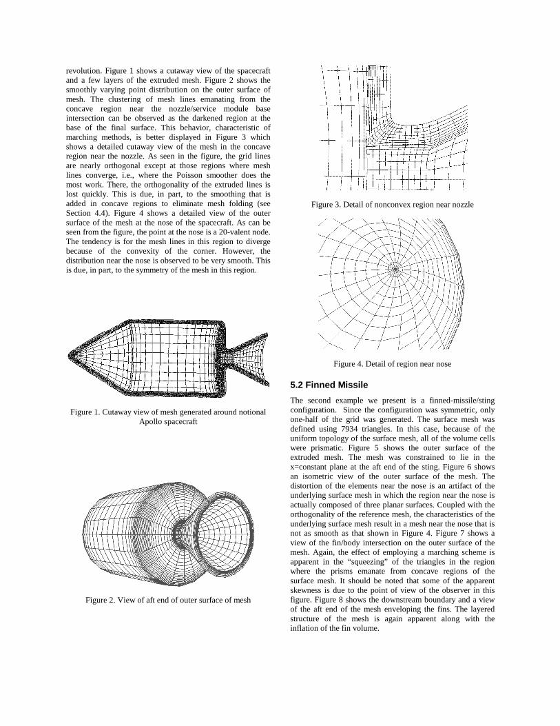
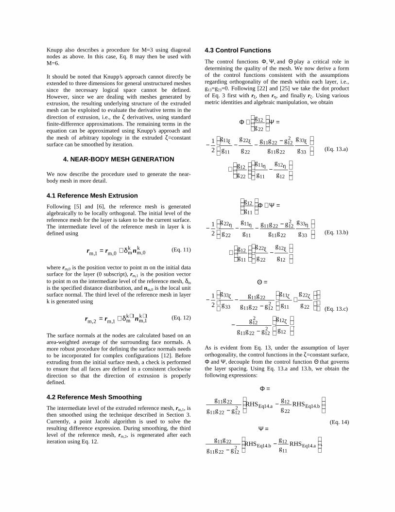
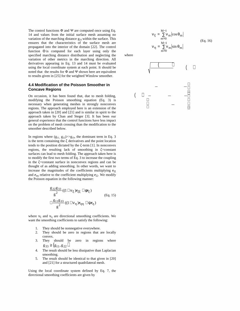
revolution. Figure 1 shows a cutaway view of the spacecraft and a few layers of the extruded mesh. Figure 2 shows the smoothly varying point distribution on the outer surface of mesh. The clustering of mesh lines emanating from the concave region near the nozzle/service module base intersection can be observed as the darkened region at the base of the final surface. This behavior, characteristic of marching methods, is better displayed in Figure 3 which shows a detailed cutaway view of the mesh in the concave region near the nozzle. As seen in the figure, the grid lines are nearly orthogonal except at those regions where mesh lines converge, i.e., where the Poisson smoother does the most work. There, the orthogonality of the extruded lines is lost quickly. This is due, in part, to the smoothing that is added in concave regions to eliminate mesh folding (see Section 4.4). Figure 4 shows a detailed view of the outer surface of the mesh at the nose of the spacecraft. As can be seen from the figure, the point at the nose is a 20-valent node. The tendency is for the mesh lines in this region to diverge because of the convexity of the corner. However, the distribution near the nose is observed to be very smooth. This is due, in part, to the symmetry of the mesh in this region.

Figure 1. Cutaway view of mesh generated around notional

Apollo spacecraft

Figure 2. View of aft end of outer surface of mesh

Figure 3. Detail of nonconvex region near nozzle

Figure 4. Detail of region near nose

5.2 Finned Missile

The second example we present is a finned-missile/sting configuration. Since the configuration was symmetric, only one-half of the grid was generated. The surface mesh was defined using 7934 triangles. In this case, because of the uniform topology of the surface mesh, all of the volume cells were prismatic. Figure 5 shows the outer surface of the extruded mesh. The mesh was constrained to lie in the x=constant plane at the aft end of the sting. Figure 6 shows an isometric view of the outer surface of the mesh. The distortion of the elements near the nose is an artifact of the underlying surface mesh in which the region near the nose is actually composed of three planar surfaces. Coupled with the orthogonality of the reference mesh, the characteristics of the underlying surface mesh result in a mesh near the nose that is not as smooth as that shown in Figure 4. Figure 7 shows a view of the fin/body intersection on the outer surface of the mesh. Again, the effect of employing a marching scheme is apparent in the “squeezing” of the triangles in the region where the prisms emanate from concave regions of the surface mesh. It should be noted that some of the apparent skewness is due to the point of view of the observer in this figure. Figure 8 shows the downstream boundary and a view of the aft end of the mesh enveloping the fins. The layered structure of the mesh is again apparent along with the inflation of the fin volume.

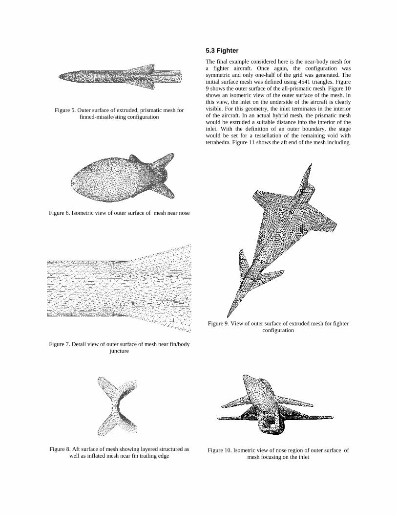
Figure 5. Outer surface of extruded, prismatic mesh for

finned-missile/sting configuration

Figure 6. Isometric view of outer surface of mesh near nose

Figure 7. Detail view of outer surface of mesh near fin/body juncture

Figure 8. Aft surface of mesh showing layered structured as well as inflated mesh near fin trailing edge

5.3 Fighter

The final example considered here is the near-body mesh for a fighter aircraft. Once again, the configuration was symmetric and only one-half of the grid was generated. The initial surface mesh was defined using 4541 triangles. Figure 9 shows the outer surface of the all-prismatic mesh. Figure 10 shows an isometric view of the outer surface of the mesh. In this view, the inlet on the underside of the aircraft is clearly visible. For this geometry, the inlet terminates in the interior of the aircraft. In an actual hybrid mesh, the prismatic mesh would be extruded a suitable distance into the interior of the inlet. With the definition of an outer boundary, the stage would be set for a tessellation of the remaining void with tetrahedra. Figure 11 shows the aft end of the mesh including

Figure 9. View of outer surface of extruded mesh for fighter

configuration

Figure 10. Isometric view of nose region of outer surface of

mesh focusing on the inlet

Figure 11. Aft end of fighter mesh

Figure 12. Detail view of aft end of inlet the region near the trailing edges of the wing and tail. Figure 12 shows a detailed view of the aft end of the inlet. The upward turning of the lines on the sidewall near the aft plane is an artifact of the underlying surface mesh.

6. CONCLUSIONS

The capability to generate prismatic and hexahedral volume meshes from surface meshes of arbitrary topology has been demonstrated. The locally three-dimensional nature of the mesh generation algorithm allows it to be used for complex surfaces with convex and concave regions. Further, the resulting mesh can be thought of as nearly orthogonal since it is generated in layers by smoothing an orthogonal reference mesh. This algorithm borrows heavily from parabolic grid generation methods for structured grids as well as smoothing methods for unstructured quadrilateral methods. This near-body mesh generation algorithm is but one of the steps in a fully generalized grid generation methodology for complex configurations. The primary advantage of this approach is that meshes of arbitrary topology may be used to discretize the surface of the configuration under consideration. This capability opens the door for highly efficient, mixed topology surface meshes to be used resulting in accurate simulations of viscous flows for complex configurations.

ACKNOWLEDGEMENTS

The partial support provided by NASA Glenn Research Center under grant NAG3-2235, Yung Choo Technical Monitor, and by the Mississippi State University/National Science Foundation Engineering Research Center is gratefully acknowledged.

REFERENCES

[1] J. F. Thompson, Z. U. A. Warsi, and C. W. Mastin, Numerical Grid Generation: Foundations and Applications, North Holland, New York, NY, 1985.

[2] S. P. Spekreijse, “Elliptic Grid Generation Based on Laplace Equations and Algebraic Transformations,” J. Comp. Phys.,Vol. 118, pp. 38-61, 1995.

[3] W. M. Chan and J. L. Steger, “Enhancements of a Three-Dimensional Hyperbolic Grid Generation Scheme,” Appl. Math. Comput., Vol. 51, pp.181-205, 1992.

[4] S. Nakamura, “Marching Grid Generation Using Parabolic Partial Differential Equations,” Numerical Grid Generation, Ed. J. F. Thompson, Elsevier Science Publishing Company, Inc., New York, pp. 775-786, 1982.

[5] R. W. Noack and D. A. Anderson, “Solution-Adaptive Grid Generation using Parabolic Partial Differential Equations,” AIAA J., Vol. 28, pp.1016-1023, 1990.

[6] R. W. Noack, and I. H. Parpia, “Solution Adaptive Parabolic Grid Generation in Two and Three Dimensions,” Numerical Grid Generation in Computational Fluid Dynamics and Related Fields, Eds. A. S.-Arcilla, J. Hauser, P. R. Eiseman, and J. F. Thompson, Elsevier Science Publishing Company, New York, pp. 475-484, 1991.

[7] N. P. Weatherill, “A Method for Generating Irregular Computational Grids in Multiply Connected Planar Domains,” Int. J. Num. Methods Fluids, Vol. 8, pp. 181-197, 1988.

[8] N. P. Weatherill and O. Hassan, “Efficient Three-Dimensional Delaunay Triangulation with Automatic Point Creation and Imposed Boundary Constraints,” Int. J. Num. Methods Eng., Vol. 37, 1994, pp. 2005-2039.

[9] D. L. Marcum and N. P. Weatherill, “Unstructured Grid Generation Using Iterative Point Insertion and Local Reconnection,” AIAA J., Vol. 33, p. 1619-1625, 1995.

[10] J. A. Shaw, “Hybrid Grids,” Handbook of Grid Generation, Eds. J. F Thompson, B. K. Soni, and N. P. Weatherill, CRC Press, Boca Raton, FL, 1998.

[11] J. A. Chappell, J. A. Shaw, M. Leatham, “The Generation of Hybrid Grids Incorporating Prismatic Regions for Viscous Flow Calculations,” Numerical Grid Generation in Computational Field Simulation, Eds. M. Cross, B. K. Soni, J. F. Thompson, J. Hauser, and P. R. Eiseman, NSF Engineering Research Center for Computational Field Simulations, Mississippi State, MS, pp. 537-546, 1996.

[12] Y. Kallinderis, “Hybrid Grids and Their Applications,” Handbook of Grid Generation, Eds. J. F Thompson, B. K. Soni, and N. P. Weatherill, CRC Press, Boca Raton, FL, 1998.

[13] C.-T. Huang, “Hybrid Grid Generation System,” M.S. Thesis, Department of Aerospace Engineering, Mississippi State University, 1996.

[14] J. L. Steger, “Generation of Three-Dimensional Body-Fitted Grids by Solving Hyperbolic Partial Differential Equations, ” NASA TM 101069, January 1989.

[15] K. Matsuno, “Hyperbolic Upwind Method for Prismatic Grid Generation, ” AIAA Paper 2000-1003, Presented at AIAA 39th Aerospace Sciences Meeting, Reno, NV, January 2000.

[16] T. C. Wey, “The Application of an Unstructured Grid Based Overset Grid Scheme to Applied Aerodynamics,” Proc. 8th Int. Meshing Roundtable ‘99, Sandia National Laboratories, pp. 163-169, 1999.

[17] T. Blacker, “The Cooper Tool,” Proc. 5th Int. Meshing Roundtable ‘96, Sandia National Laboratories, pp. 13-29, 1996.

[18] M. L. Staten, S. A. Cannan, and S. J Owen, “BMSweep: Locating Interior Nodes During Sweeping,” Proc. 7th Int. Meshing Roundtable ‘98, Sandia National Laboratories, pp. 7-18, 1998.

[19] P. M. Knupp, “Next-Generation Sweep Tool: A Method for Generation All-Hex Meshes on Two-and-One-Half Dimensional Geometries,” Proc. 7th Int. Meshing Roundtable ‘98, Sandia National Laboratories, pp. 505-513, 1998.

[20] D. S. Thompson and B. K. Soni, “Generation of Quad- and Hex-Dominant, Semistructured Grids using an Advancing Layer Scheme,” Proc. 8th Int. Meshing Roundtable 1999, Sandia National Laboratories, pp. 171-178, 1999.

[21] D. S. Thompson and B. K. Soni, “Semistructured Grid Generation in Three Dimensions using a Parabolic Marching Scheme,” AIAA Paper 2000-1004, Presented at 38th Aerospace Sciences Meeting, Reno, NV, January 2000.

[22] P. Knupp, “Applications of Mesh Smoothing: Copy, Morph, and Sweep on Unstructured Quadrilateral Meshes,” Int. J. Num. Meth. Eng., Vol. 45, pp. 37-45, 1999.

[23] A. Winslow, “Numerical Solution of the Quasilinear Poisson Equations in a Nonuniform Triangular Mesh, ” J. Comp. Phys., Vol. 2, pp. 149-172, 1967.

[24] P. M. Knupp, “Winslow Smoothing on Two-Dimensional Unstructured Meshes,” Proc. 7th Int. Meshing Roundtable ‘98, Sandia National Laboratories, pp. 449-457, 1998.

[25] B. K. Soni, “Elliptic Mesh Generation Systems: Control Functions Revisited,” App. Math. Comp., Vol. 59, pp.151-164, 1993.

[26] “Cobalt60 On-Line Documentation,” Cobalt60, September 1999, http://www.va.afrl.af.mil/vaa/ vaac/COBALT/co_docs.html.

[27] EnSight User Manual for Version 6.2, Computational Engineering International, Inc.