generation of squeezed light via second harmonic generation
TRANSCRIPT
)
Generation of Squeezed Light Via SecondHarmonic Generation
by
Philip Tsefung Nee
Submitted to the Department of Electrical Engineering andComputer Science
in partial fulfillment of the requirements for the degree of
Master of Science in Electrical Engineering and Computer Science
at .the
MASSACHUSETTS INSTITUTE OF TECHNOLOGY
February 1994
( Phillip Tsefung Nee, MCMXCIV. All rights reserved.
The author hereby grants to MIT permission to reproduce anddistribute publicly paper and electronic copies of this thesis
document in whole or in part, and to grant others the right to do so.
Author ..... ..........
Department of Electricalg ngineering and Computer ScienceJanuary 24, 1994
Certified by... .W- T.
Leader, Optical Communications Technology
K\ A M . ,
Accepted by.......
Chairman,
Dr. Roy BondurantGroup, MIT Lincoln
LaboratoryThesis Supervisor
Committ
'BI8ARiES
_&, .

Generation of Squeezed Light Via Second Harmonic
Generation
by
Phillip Tsefung Nee
Submitted to the Department of Electrical Engineering and Computer Scienceon January 14, 1994, in partial fulfillment of the
requirements for the degree ofMaster of Science in Electrical Engineering and Computer Science
AbstractThe purpose of this thesis is to assess the feasibility of using semiconductor lasersand a monolithic KNbO 3 cavity to generate squeezed states of light. An experi-mental setup designed to detect amplitude squeezing via second harmonic generationfrom a doubly resonant KNbO 3 monolithic cavity was constructed. Based on the ex-perimentally determined cavity parameters, a critical power of 3.5mW and a criticalfrequency of 400MHz are predicted. The maximum achievable amount of amplitudesqueezing at an input power equal to the predicted critical power is determined tobe 31% at the fundamental and 79% at the second harmonic. Excess noise from thediode laser prevented observation of squeezing.
Thesis Supervisor: Dr. Roy BondurantTitle: Leader, Optical Communications Technology Group, MIT Lincoln Laboratory

Acknowledgments
First and foremost, I would like to thank Roy Bondurant, my research advisor, for
affording me the oppotunity to work on this project and for providing me with con-
tinued guidance throughout the course of the project. I'd also like to express my
gratitude to my supervisor Jeff Livas, from whom I learned an inordinate amount of
practical knowledge and skills from a variety of fields. Above all, I'd like to thank
him for his guidance and support throughout the course of the project and for being a
truly classy individual to work with. Then I'd like to express my heart-felt thanks to
Josephine Cappiello for constructing and repairing a number of much-needed hard-
ware for the experiment and for providing generous technical assistance whenever
I needed it. Then there's Fred Walther, whom I'd like to thank for lending me a
paraphernalia of instruments and devices such as the 100mW diode laser, the blue
filter, and the one-pass KNbO 3 crystal. I'd like to thank Ron Sprague for making the
mounts for the crystal and helping me with a variety of machining jobs. I'd like to
thank Jean Mead for the various secretarial help such as scheduling talks and typing
up memos. Among others to whom I'd like to say thanks are Eric Swanson, Laura
Adams, David Cruciolli, Fred Beihold, and Al Tidd for their generosity in lending me
a variety of tools, instruments, and devices.
Contents
1 Introduction
1.1 Thesis Outline . ......................
1.2 Squeezed States . . . . . . . . . . . . . . . . .
1.2.1 Qualitative description . . . . . . . . . . . . . .
1.2.2 Applications of squeezed states of light .....
1.3 Methods of Generating Squeezed Light .........
1.3.1 Possible Methods In General ............
1.3.2 Past Experimental Accomplishments By Others
1.4 Motivation and general features for this work ......
2 Generation of Squeezed States Via SHG Inside a Doubly
Cavity
2.1 Mathematical Description of Second Harmonic Generation
2.2 Phasematching .........................
2.2.1 Phasematching by temperature ............
2.2.2 Phasematching by electro-optic effect .........
2.3 SHG Inside A Doubly Resonant Cavity ............
2.3.1 Achieving double-resonance and phasematching . . .
2.3.2 Equations of motion . . . . . . . . . . . . .
2.4 Amplitude squeezing via SHG .................
Resonant
14
14
16
17
17
18
18
19
21
3 Experimental Setup And Procedure
4 Alignment of Crystal
24
26
4
6
6
7
7
8
8
8
10
11
4.1 Linear vs. Ring Resonator ........................ 26
4.2 Modematching .............................. 27
5 Determining Cavity Losses 29
5.1 Expression for Cavity Bandwidth .................... 29
5.2 Measurement of Cavity Bandwidth-Fundamental Mode ....... 30
5.3 Measurement of Cavity Bandwidth-Second Harmonic Mode ..... 31
6 Achieving Double Resonance Via Frequency Locking 33
6.1 The Pound-Drever Locking Scheme ................... 33
6.2 Locking the Second Harmonic Intensity ................. 35
6.3 Thermal Effect .............................. 36
6.3.1 Asymmetry in SH intensity as a function of temperature . . . 36
6.3.2 Asymmetry in SH intensity as a function of electro-optic voltage 37
7 Noise Measurement and Analysis 38
7.1 Shot Noise, Thermal Noise, RIN, and Amplifier Noise ......... 38
7.2 Noise Measurement Results ....................... 41
7.3 Mode Partition Noise ........................... 43
8 Determination of Coupling Coefficient K And Critical Power 44
8.1 Measurement of Coupling Coefficient ................. 44
8.2 Dependence of Critical Power/Critical Frequency on Frequency Detun-
ings .................................... 46
8.3 Experimental Determination of Critical Power ............. 47
9 Detection Of Amplitude Squeezing 49
10 Conclusion 51
5

Chapter 1
Introduction
Random fluctuations of electromagnetic fields, dictated by the uncertainty principle
in quantum mechanics, set the ultimate limit on the amount of precision possible
in transmitting information by photons, or light. It is anticipated that, in the near
future, many communications sytems which use light to transmit information will
progress to the point where the accuracy of the transmitted information is limited by
the random fluctuations in the optical field. Is there a way to reduce such fluctuations?
Squeezed light allows one to redistribute the noise in an optical field such that the
noise in one component of the field is less than that for classical light while the noise
in the other component exceeds that of classical light. This offers the potential for
using only the squeezed part of the light to transmit the information, thus improving
the precision beyond that for classical light.
1.1 Thesis Outline
This thesis describes an experimental setup aimed at generating squeezed light from
a potassium niobate crystal via the nonlinear optical process of second harmonic gen-
eration. The thesis is organized into the following chapters. The rest of this chapter
consists of three sections. Section 1.2 provides a qualitative description of squeezing.
In particular, a distinction is drawn between quadrature and amplitude squeezing.
Also, some potential applications of squeezed light are discussed. In section 1.3 the
6

various physical processes that produce squeezed light are described, followed by a
discussion of past experimental results by others in the generation of squeezed light.
Section 1.4 discusses the motivation and general features of this experiment. Chapter
2 provides an extensive treatment of squeezing via second harmonic generation inside
a doubly resonant cavity. The experimental setup is described in Chapter 3. Chapters
4 through 9 outlines the general progress of the experiment. The results achieved in
the experiment will also be discussed in these chapters. A summary of the experiment
and the results will be included in Chapter 10 along with a few concluding remarks.
1.2 Squeezed States
1.2.1 Qualitative description
At a given point in space a monochromatic electromagnetic wave of frequency w can
be specified by its amplitude and phase or by its sine and cosine components:
E(t) = Acos(wt + )
E(t) = acoswt + bsinwt (1.1)
According to quantum theory, the two components A, qb or a, b that specify the field
are noncommuting operators and are therefore subject to the constraints of Heisen-
berg's uncertainty principle. That is, the two components cannot be known with
absolute certainty simultaneously. In fact the product of their uncertainties must
always be equal to or larger than a fundamental constant proportional to Planck's
constant h. It is possible, however, to manipulate the field in such a way that the un-
certainty in one component is reduced at the expense of increasing the uncertainty in
the other component while the product of their uncertainties remain unchanged. The
component whose uncertainty is reduced is appropriately described as the "squeezed"
component [28].
In classical light, such as light emitted by a coherent laser, the uncertainties in the
7

sine and cosine components of the field are equal, and the uncertainty in the amplitude
of the field obeys a Poisson distribution. In quadrature-squeezed light the uncertainty
in either the sine or cosine component is decreased while that in the other component
is correspondingly increased. In amplitude-squeezed light, the uncertainty in the
intensity number is reduced to below the shot noise limit characteristic of classical
light at the expense of increasing the uncertainty in the phase of the field. It is
also possible to generate phase-squeezed light, the direct counterpart to amplitude-
squeezed light.
1.2.2 Applications of squeezed states of light
Amplitude-squeezed light finds potential use in communications systems or in mea-
surements that require very high precision[28][22]. In optical communications sys-
tems, for example, the information to be transmitted can be encoded on the amplitude
(squeezed) quadrature of light. A detection scheme that is sensitive to the amplitude
but not to the phase of the transmitted light would then record the information and
thus improve the signal-to-noise ratio beyond that for a shot-noise-limited system.
Other applications of squeezed light involve areas such as gravitational wave detec-
tion and optical ring gyroscope, where squeezed light offers a potential improvement
by increasing the sensitivity of the detection scheme.
1.3 Methods of Generating Squeezed Light
1.3.1 Possible Methods In General
Experimentally, squeezed states of light have been generated since 1985[30]. Both
quadrature-squeezed and amplitude-squeezed light have been produced by a variety
of experimental configurations. Up to the present squeezed light has been generated
by various forms of three-wave or four-wave mixing nonlinear optical processes and
also by diode laser outputs which are below shot-noise[31][14]. In a four-wave mixing
process, as shown in Figure la, four lightwaves interact via a nonlinear medium. The
8

nonlinear medium is often in the form of a nonlinear crystal, but the medium can
be gaseous or liquid as well. Two strong counterpropagating pump fields El, E2 of
angular frequencies wl, W2 and two other fields E3, E 4 of frequencies w3, w4 interact
in the nonlinear medium. The fields obey energy conservation w1 + w2 = W3 + w4 and
momentum conservation kl + ck2 = 1c3 + kc4 . Assuming w1 = w2 = w, a weak input field
E 3 of frequency w will give rise to an output field E 4 whose frequency is w4 = w and
whose complex amplitude is everywhere the complex conjugate of E3. Adding the two
fields E3 and E4 interferometrically results in a new field that is quadrature-squeezed.
The general class of nonlinear optical processes called three-wave mixing has also
produced both quadrature- and amplitude-squeezed light. Some of the best results in
squeezing were achieved with optical parametric oscillation. In optical parametric os-
cillation (Figure lb) an input field of frequency wp interacts with a nonlinear medium
to produce two output fields of frequencies 1o and w2 such that wp = Wo + w2. In
the so-called dengerate optical parametric oscillator, w1 = 2 = 1wp. Anticorrelation
in the distribution of photons from the two output fields gives rise to quadrature- or
amplitude-squeezing in the two output fields. The type of squeezing that is manifested
depends on the specific detection scheme used.
Second harmonic generation, another three-wave mixing process, has also been
employed to generate amplitude-squeezed light. In second harmonic generation (Fig-
ure lc) an input field at frequency w gives rise to a second field at frequency 2w inside
a nonlinear medium. The output consists of both the second harmonic field and a
residual field at the fundamental frequency w. The nonlinear interactions introduce
anticorrelation in the distribution of photons in both the fundamental and the sec-
ond harmonic output fields such that both fields are amplitude-squeezed. Second
harmonic generation is the method used in this work for generating squeezed light.
A more detailed discussion of amplitude-squeezeing via second harmonic generation
follows in the next chapter.
9

1.3.2 Past Experimental Accomplishments By Others
The first experimental demonstration of squeezed light was achieved by R. Slusher
et. al. in 1985[26]. In their setup quadrature-squeezed light was generated by non-
degenerate four-wave mixing due to sodium atoms in an optical cavity. A balanced
homodyne detection system was used to measure the quadrature components of the
output beam from the cavity. It was found that the fluctuation of one of the two
quadratures was below the vacuum noise level. A modest amount of noise reduc-
tion (7%) below shot noise level was observed. Several other groups also generated
squeezed states around the same time, all involving four-wave mixing of some kind
but showing only modest amounts of noise reduction[15][23][21].
The most spectacular results in squeezing to date involve the process of parametric
downconversion as described in the previous section. Wu et. al. demonstrated a
60% reduction in quadrature noise below the shot noise level in 1987[29][30]. In
their setup the output of a Nd:YAG laser at a wavelength of A = 1062nm was
frequency doubled inside a Ba 2NaNb 5 015 crystal to generate a second harmonic beam
at A = 531nm. This beam served as the pump field to the optical parametric oscillator.
A lithium niobate crystal doped with magnesium oxide (LiNbO 3 :MgO) was used as
the nonlinear medium for parametric downconversion. The crystal was placed inside
an external cavity to increase the efficiency of conversion. The quadrature-squeezed
signal field was then detected by balanced homodyne detection.
In 1989 T. Debuisschert et. al. reported a setup that exploits the anticorrelation
in photon distribution between the signal and idler outputs generated by a non-
degenerate optical parametric oscillator[4]. A noise reduction of 69% was observed in
the difference in the intensities of the signal and idler outputs. Amplitude squeezing
was generated in this case, since the noise reduction involves the relative intensities of
the two outputs. The pump field was driven by an argon ion laser at a wavelength of
A = 528nm. The optical parametric oscillator consists of a KTP crystal placed inside
an external cavity. The wavelengths of the signal and idler fields were at A, = 1048nm
and Ai = 1067nm, respectively. The two output fields were separated by a polarizer
and detected by separate photodetectors. Intensity noise reduction below the shot
10
noise level in the difference between the two photodetector outputs was then observed
on a spectrum analyzer. Other published results in squeezing using the parametric
downconversion process are given in the bibliography[25] [7] [27] [16] [17].
Squeezing via second harmonic generation was first reported by S. Periera et. al.
in 1988[18]. Their setup consists of a LiNbO 3:MgO crystal placed inside an external
cavity and pumped by a Nd:YAG laser at a wavelength of A = 1062nm. A second
harmonic output beam at a wavelength of A = 531nm was generated. The reflected
fundamental field was detected, and a 13 % reduction in the intensity fluctuation
below the shot noise level was observed.
More recently, in 1992, Kurtz et. al. reported a 40% reduction in the intensity
fluctuation of the second harmonic mode below the shot noise level[24][11]. In their
setup a monolithic LiNbO 3:MgO cavity was used as the medium for second harmonic
generation. The pump field at A = 1062nm was generated by a Nd:YAG laser. The
ends of the crystal were coated to resonate strongly at both the fundamental and the
second harmonic wavelengths. The transmitted second harmonic output field was
detected by balanced homodyne detection.
In the aforementioned setups involving squeezing via second harmonic generation,
the nature of the squeezing generated is amplitude squeezing, since the second har-
monic generation process introduces anticorrelation in the photon number distribution
at both the fundamental and second harmonic wavelengths.
1.4 Motivation and general features for this work
As mentioned previously, this work involves the generation of amplitude-squeezed
light via second harmonic generation inside a doubly resonant cavity. In this partic-
ular setup a monolithic cavity made up of potassium niobate (KNbO 3 ) serves as the
nonlinear medium for second harmonic generation. The pump field is produced by
a diode laser operating at a wavelength of A = 860nm. The monolithic cavity is de-
signed such that significant amplitude squeezing is expected at both the fundamental
and the second harmonic wavelengths.
11

The primary motivation for this work is to design a setup that allows one to
produce a compact, efficient, and relatively inexpensive source of squeezed light that
may ultimately find use in optical communication systems. The diode laser's size
and cost, compared to those of other laser systems, make it the natural candidate for
such purposes. The use of KNbO 3 as the nonlinear medium provides two additional
advantages. First, the limited output power of the diode laser makes it imperative
that a material with a high optical nonlinearity be used. KNbO 3 possesses a strong
nonlinear optical coefficient that significantly exceeds that of most other commonly
used nonlinear materials such as LiNbO 3:MgO and KTP. As discussed in the previ-
ous chapter, there is an optimum power level (the critical power) at which the largest
amount of squeezing can be generated. For KNbO 3 the critical power level is quite
low, on the order of a few milliwatts. Of course, the critical power is also a sensi-
tive function of the cavity loss rates at the fundamental and at the second harmonic
wavelengths. Second, the phasematching temperature for KNbO 3 at a wavelength
of A = 860nm is around room temperature. Consequently, there is no need to heat
the crystal to high temperatures, as is the case for systems involving LiNbO 3, where
the phasematching temperature at A = 1062nm is about 123°C. The phasematching
consideration is also the main reason for selecting A = 860nm as the wavelength for
the pump field.
Table 1 provides a summary of the general features of past accomplishments in
squeezing via second harmonic generation and of the work described by this thesis.
12

Table 1. Experiments Involving Squeezing ViaTT * /" j
Second
Harmonic enerationFeatures Pereiva et. al. Kurz et. al. This work
(1988) (1992)
Material LiNbO3:MgO LiNbO3 :MgO KNbO 3
Cavity design external monolithic monolithic
Type of laser Nd:YAG Nd:YAG diode
Wavelength 1062nm 1062nm 860nm
Phasematching temperature 123°C 123°C 27°C
Critical power 1.6W 200mW 3.5mW
Observed squeezing 13% 40% -
13
Chapter 2
Generation of Squeezed States Via
SHG Inside a Doubly Resonant
Cavity
The observation of second harmonic generation in the early 1960's marked the birth
of nonlinear optics. Second harmonic generation is the most fundamental and best
understood optical nonlinear interaction. In this chapter the basic theory of second
harmonic generation and a number of practical issues in nonlinear optics such as
phasematching and the use of a resonator to generate second harmonic generation
are discussed.
2.1 Mathematical Description of Second Harmonic
Generation
In a nonlinear medium the electric field of the incident radiation induces a nonlinear
polarization whose magnitude and phase are given by the product of the incident
fields. The expression for the nonlinear polarization is given as follows[31, p. 384]:
Pi = EoxijEj + 2odijkEjEk + 4EodijklEjEkE + .... (2.1)
14

where Xij is the linear susceptibility tensor, and dijk, dijkl ..... are the optical non-
linearity tensors that relates the induced nonlinear polarization to the products of
the incident fields. In the special case of second harmonic generation, the relevant
nonlinear polarization is
Pi(w2 ) = odijkEj(Wl)Ek(Wl) (2.2)
where w2 = 2w1 [5]. The subscript i refers to the cartesian components of the polar-
ization vector.
From Maxwell's equations with the constitutive relation
D = EE + Pinar,, + Pnonlinear (2.3)
one obtains the wave equation
0 02 -02 -((V 2 - - e -o )E(2W) = o2PNL(2W) (2.4)
Mathematically the nonlinear polarization serves as the source term in the wave
equation for the second harmonic field. Assuming the fields propagate in the z-
direction and ignoring propagation losses, the steady state second harmonic field
amplitude is related to the fundamental field amplitude by
a (2w) = -j OdCff(w)()exp[(k - k)z]TZ 2n
where kp = 2k(w), k = k(2w), and dff is the effective nonlinear coefficient. Note also
that the field amplitude E is related to the total field E by
E(z, t) = E(z)exp(jkz - wt) (2.6)
15

2.2 Phasematching
Integrating (2.5) one can determine the second harmonic field amplitude as a function
of distance. The conversion efficiency to the second harmonic is optimized when the
two fields are phasedmatched. That is, when k(2w) = 2k(w) or n(2w) = 2n(w),
where n, the refractive index, is related to k by k = 2, A being the wavelength.
Physically, phasematching describes the condition at which the phase velocities of the
fundamental and the second harmonic fields are identical. For most commonly used
nonlinear materials, the index of refraction can be tuned by a number of parameters:
frequency (wavelength), temperature, orientation of the crystal axes with respect to
the incident wave, and electric field. In this work, the indices of refraction at the
fundamental and the second harmonic wavelengths are adjusted by temperature and
by an applied field across the nonlinear medium. The orientation of the crystal axes
with respect to the incident wave is fixed.
In normally dispersive materials the index of refraction decreases with the wave-
length of the field[31, p. 394]. In anisotropic materials two independent propagation
modes exist, each with a different index of refraction[31, p. 87]. The two modes cor-
respond to two orthogonally polarized electric displacement vectors D. The direction
of propagation specified by the k vector is normal to the plane formed by the two
allowed D vectors. Figure 2 shows how phasematching is possible. Provided that
the fundamental and second harmonic fields are polarized orthogonally to each other
and thus corresopond to the two independent popagation modes, phasematching is
achieved when the index of one mode at the fundamental wavelength is matched to
the index of the other mode at the second harmonic wavelength. The tuning curve of
one of the modes, the so-called extraordinary mode, is a function of the orientation
of the crystal axes with respect to the incident wave[31, p. 92]. While the orientation
is fixed in this experiment because of the use of a monolithic cavity, it is a tuning pa-
rameter for phasematching in many other applications. Figure 3 shows the nonlinear
KNbO3 crystal employed in this experiment and its corresponding crystal axes. The
crystal is biaxial with principal indices of refraction n, < n, < nb[1]. The indices of
16

refraction of the two propagation modes can be determined from the principal indices
of refraction using the index ellipsoid method[31, p. 90]. The incident light propagates
along the a-axis and is polarized along the b-axis. The transmitted second harmonic
field is polarized along the c-axis, while the transmitted fundamental field remains
polarized along the b-axis. The two independent modes of propagation correspond
to the b-polarized fundamental wave and the c-polarized second harmonic wave with
indices of refraction nb and no, respectively.
2.2.1 Phasematching by temperature
To satisfy the phasematching condition the condition nb(w) = n0 (2w) must be sat-
isfied. In general, both indices of refraction are functions of temperature. That is,
nb(w) = nb(w, T) and n,(w) = n,(w, T). Shown in Figure 4 is the dependence of the
indices of refraction as a function of temperature for KNbO 3 at a wavelength A = 860
nm (or w = 2.19 x 10¹⁵/s). It is clear from the figure the phasematching condition
is satisfied around 270 C. It should be emphasized that Figure 4 is valid only at a
wavelength of A = 860nm. The phasematching temperature of KNbO 3 is a sensitive
function of wavelength, as shown in Figure 5.
2.2.2 Phasematching by electro-optic effect
The index of refraction of a nonlinear material can also be tuned by applying a dc
electric field. This effect is called the electro-optic effect. The change in the index of
refraction is related to the applied field by the following equation[31]:
1 1
2(n..j 2n rijEk (2.7)
Here rijk is the (third-ranked) electro-optic tensor, and the cartesian coordinate sys-
tem is that of the crystal axes of the nonlinear material. The indicies of refraction
are given as tensor elements in the above equation. To find the change in index of
refraction along a given direction, one must diagonalize the 3 x 3 tensor and determine
the new set of principal axes, which is generally different from the crystal axes of the
17

nonlinear material. Assoicated with each principal axis is a new index that may be
a function of the applied electric field. The projection of the direction of interest on
the principal axes allows one to determine the index for a field polarized along that
direction. For an electric field applied across the c-axis as shown, the electro-optic
tensors that contribute to the index change are r 3, r 123, r133, r223, r233 and r333 In
the case of KNbO 3, all of the above tensor elements are identically zero except for
r 333. Therefore, the change in index is entirely along the c-axis, implying that n,(2w)
can be adjusted independently of nb(w) by the applied field. This is not the case for
temperature tuning, where both n¢(2w) and nb(w) vary with temperature.
2.3 SHG Inside A Doubly Resonant Cavity
In general the efficiency of second harmonic generation from a single pass crystal is
rather limited. One way to improve the efficiency of second harmonic generation is to
place the nonlinear crystal inside an optical resonator. In a resonator, light essentially
makes many passes through the nonlinear crystal before leaving the resonator, thereby
effectively increasing the interaction length. Furthermore, "mirrors" can be directly
deposited on the end facets of the crystal to form a resonator, such that physically the
crystal and the cavity are identical. Such "mirrors" are usually realized by depositing
a dielectric that is highly reflecting at the wavelength(s) of interest onto the crystal.
This type of cavity is commonly referred to as a monolithic cavity. In this experiment
a KNbO 3 monolithic cavity that is resonant at both the fundamental and the second
harmonic wavelengths is employed. The rest of the section will be devoted to a
discussion of second harmonic generation inside a doubly resonant cavity.
2.3.1 Achieving double-resonance and phasematching
At double-resonance the roundtrip phase of the fundamental and second harmonic
fields must each be integer multiples of 27r:
2=rnb-'4s = Ik(W)l = T = 2rNA\
18

2'rnTc2 w2 = k(2w)l = -2-rM (2.8)
Here N, M are integers, and I is the length of the crystal. n 2 0 and nbW are indices of
refraction of the second harmonic field polarized along the c- and b-axis, respectively.
To satisfy the double-resonance and phase-matching conditions simultaneously, one
setsnb N-- =-'1n, 2 2M
By definition the two refractive indices are equal under phasematched condition.
However, phasematching is a sufficient but not a necessary condition for double reso-
nance, provided that the physical cavity length is identical for the two fields. Double
resonance can be achieved without phasematching (i.e. N 4 2M), the penalty being
reduced conversion efficiency to the second harmonic compared to the phasematched
case.
2.3.2 Equations of motion
The semi-classical equations of motion describing second harmonic generation inside
a Fabry-Perot resonator are[5]:
dt1 = j Al C 1 -- 71 a1 + Ka;a 2 + 1
d = j - (2.9)denotes the complex conjugate. Here normalized electric field amplitudes
where * denotes the complex conjugate. Here normalized electric field amplitudes
cal, a 2, corresponding to the fundamental and second harmonic modes, respectively,
are used. el is the pump amplitude at the fundamental frequency. 71 and 72 are the
cavity loss rates for the two modes, and Al, A2 are frequency detunings from the
resonant frequencies of the two modes. The parameter r. is the coupling coefficient
between the two fields. It determines the amount of energy transfer between the two
fields. Experimental determination of 71, 72, and s is treated in Chapters 5 and 9.
19

The normalized field amplitudes are related to the actual field amplitudes by
£ = 3jr 2w (2.10)
where V is the mode volume, and hv is the energy of a single photon of frequency v.
The equations of motion can be linearized around the steady state fields inside the
cavity. In obtaining the steady state, one setsdal = 0 and d 2 = 0 and solves fordt CYI dt/2 - and s ve s frtthe al and a 2. The second harmonic amplitude can be shown to be a single-valued
function of the normalized driving field E1:
2 2 Ca2 13 + 4l721ca 2 12 + 2l 2 Y2 Ka 2I = I rl2 (2.11)
Here we have assumed zero detunings for simplicity. By carrying out an eigenvalue
analysis of the equations of motion around the steady state operating point, one
can show that the second harmonic mode becomes unstable and exhibits self-pulsing
instability above a critical pump field[5]
=2272(71 +72) (2.12)
The angular frequency at which this instability takes place is
fcrit 72(71 + 72) (2.13)
The normalized quantity e is related to the actual power (in units of Watts) by the
following expression:
pin,= hw A tflJ2 (2.14)
where At = 2n is the cavity roundtrip time; Ri, is the power reflectivity of theC
input facet at A = 860nm; n is the index at A = 860nm; and I is the cavity length.
This critical pump power is a key piece of information in the analysis of amplitude
squeezing as described in the following section.
20
2.4 Amplitude squeezing via SHG
In the quantum mechanical description, second harmonic generation involves the
simultaneous creation of one second harmonic photon and the annihilation of two
photons from the fundamental mode. The incident driving field has Poissonian pho-
ton statistics. That is, the arrival rate of photons is perfectly random, exhibiting a
Poissonian distriution:< n >n ezp[-< n >] (2.15)
n!
where < n > is the average photon number detected in a given detection time in-
terval. The second harmonic process converts photon-pairs in the fundamental mode
to second harmonic photons. The photocounting distribution of the photon-pairs is
sub-Poissonian, where its field fluctuation is less than that of the fundamental driving
field. The photocounting distribution of second harmonic photons is related to that
of the incident fundamental photons by
Pn(2w) = P2n(w) + P2n+l(W) (2.16)
since for a given detection interval n second harmonic photons can be detected given
2n or 2n + 1 fundamental photons in the same time interval. The intensity noise
can be expressed as the mean square deviation from. the average number of detected
photons in a given detection interval. That is, An = Vn2 - < n >2. For a Poissonian
distribution the uncertainty in the number of photons is equal to the average number
of photons:
An =< n >
Straightforward algebraic manipulation shows that the uncertainty in the photocount-
ing distribution of the second harmonic photons is less than that for a Poissonian
distribution. That is,
An(2w) << n(w) >
Therefore, the second harmonic field exhibits sub-Poissonian photon statistics.
21

The photon statistics of the output fundamental field are also sub-Poissonian. One
can view the second harmonic process as a process that selectively converts photons
that are spaced closely together in a given detection interval. The second harmonic
process thus removes bunched photons from the fundamental beam. This results in
a more evenly spaced distribution of photons, implying reduced fluctuation in the
average number of photons. By this argument the photon distribution is expected to
be sub-Poissonian for the output fundamental field as well.
Mathematically, from the linearized equations of motion for a doubly resonant
cavity discussed previously, the intensity fluctuation spectrum (in W/m2) of the fun-
damental and second harmonic fields can be expressed as a function of the frequency
Qf at which the spectrum is observed[10]:
/< a ,(f)l2 > =< I > (1- -Yl7l '2l + )2
/< IA I2 (Q)12 > =< I2 > (1 -72 Ia 2 D ) (2.17)
where
D2 = [I1 2+ 72(71 + ( + a2) - 2]2 + (1 + 72 + Ila21)202
Here < I >, < 12 > denote the average output intensities of the two modes. For
frequencies much higher than the cavity loss rates 71, 72 the field fluctuations ap-
proach the shot-noise value characteristic of classical light. Since high measurements
frquencies correspond to short observation time intervals, the amount of squeezing is
degraded for observation time intervals shorter than the cavity lifetimes at the fun-
damental and the second harmonic because interactions between light and the cavity
do not have time to occur. Shown in Figure 27a is a plot of the expected amplitude
squeezing spectra as a function of measurement frequency for a set of experimentally
determined parameters. Here V represents the noise powers of the fundamental and
the second harmonic modes normalized to their shot noise values. At V = 0 perfect
squeezing is obtained as the noise power approaches zero. It is clear that the choice
of frequency at which the spectrum is observed depends on one's interest in observing
22

squeezing in the fundamental mode or in the second harmonic mode. The loss rates
71, 72 depend on the coated reflectivities of the two facets and absorbtion within the
crystal, and the coupling coefficient KE is determined from the amount of depletion
of the fundamental mode power by second harmonic generation. As expected, both
the fundamental and second harmonic noise powers approach the shot noise level for
frequencies larger than the cavity bandwidth.
Amplitude squeezing is also a function of the input power to the crystal. As
mentioned in the previous section, the system exhibits self-sustained oscillations for
e > E,. The intensity fluctuation at the second harmonic wavelength decreases as is
increased until the critical power ec is reached (Figure 28c). Hence, the critical pump
power sets the power required for optimum amplitude squeezing.
A more complete discussion of the expected amount of amplitude squeezing as a
function of measurement frequency and of input power to the crystal is provided in
Chapter 9.
23
Chapter 3
Experimental Setup And
Procedure
The complete experimental setup described by this thesis is shown in Figure 6. The
diode laser output is driven by a constant current source and focused by a lens onto
the monolithic cavity. Two Faraday isolators serve the purpose of preventing back
reflections into the laser cavity. The incident beam is polarized vertically (normal
to the page). After the incident beam passes through the polarizing beam splitter,
the Faraday rotator rotates the polarization of the incident field by 45 degrees. The
half-wave plate rotates the polarization of the incident field to the horizontal orien-
tation, parallel to the b-axis of the KNbO 3 crystal. The transmitted fundamental
and second harmonic outputs from the cavity are separated by a filter and detected
by separate photodetectors. The reflected output from the cavity consists mainly
of the fundamental field. Since the Faraday rotator is a non-reciprocal device, the
reflected field, after passing back through the Faraday rotator, has orthogonal polar-
ization with respect to the incident field. The polarizing beam splitter then steers
the back-reflected field onto a photodetector. An rf synthesizer modulates the laser
output. A set of locking electronics amplifies and demodulates the photodetector
output to produce an error signal that feeds back to the laser bias current and thus
stabilizes the frequency of the incident field. This frequency stabilization scheme for
the fundamental field is commonly known as the Pound-Drever locking scheme and
24
will be discussed in more detail in Chapter 6[20].
A second set of locking electronics is used to stabilize the intensity of the second
harmonic output to its peak. That is, to maintain phasematching between the funda-
mental and the second harmonic fields. The KNbO 3 crystal is temperature-controlled
such that the two fields are in the vincinity of phasematching. A programmable high
voltage supply produces a field which fine-tunes the phasematching via the electro-
optic effect. An rf signal is superimposed on the dc field across the crystal, thereby
modulating the intensity of the transmitted second harmonic output. A portion of the
transmitted output is detected by a photodetector and then demodulated to give an
error signal that progams the high voltage supply. Further discussion of this intensity
stabilization scheme is provided in Chapter 6.
25

Chapter 4
Alignment of Crystal
4.1 Linear vs. Ring Resonator
The KNbO 3 crystal used in the experiment is configured as shown in Figure 7. The
crystal can be used as either a ring resonator or a linear resonator as shown in
the figure. The advantage of using the crystal in the ring configuration is that the
reflected beam travels a different path from that of the incident beam. Therefore, no
additional optics is necessary to separate the indident beam from the reflected beam.
The drawback of using the ring cavity resonator is that the the fundamental and the
second harmonic fields cannot be completely phasematched because the beam paths of
the two fields do not overlap. This effect is illustrated in Figure 8. While it is possible
to achieve phasematching between the fundamental and the second harmonic along
the cavity axis using temperature and electro-optic tuning, the same is not true for
the direction normal to the cavity axis (the b-axis). In the ring cavity design, parts of
the beam path for the fundamental and the second harmonic have components along
this transverse direction. Therefore, the two fields travel at different velocities inside
the crystal even if they are phasematched in the longitudinal direction. Consequently,
the two beams map out slightly different paths circulating the cavity.
Initially, the monolithic KNbO 3 crystal was set up as a ring cavity for the advan-
tages mentioned previously. However, the problem of non-overlapping beams made it
necessary to revert to the linear cavity set-up, which necessitates the addition of the
26

isolators to prevent feedback into the laser, of the polarizing beam splitter to steer the
reflected beam into the photodetector, and of the polarizer and the half-wave plate
to rotate the polarization of the reflected beam to 90 degrees relative to that of the
incident beam.
4.2 Modematching
One major difficulty encountered in the experiment involves the modematching of the
incident beam to the monolithic KNbO 3 cavity. The optimum beam waist inside a
cavity depends on the geometry and size of the cavity as well as the laser wavelength.
When modematched, the beam waist of the incident laser beam matches the optimum
beam waist defined for the particular cavity in question. This normally involves using
a carefully chosen focal lens to focus the incident beam to the desired beam waist
inside the cavity. Failure to achieve modematching results in the presence of higher-
order radial sidemodes as well as drastically reduced efficiency in the conversion to
the second harmonic.
For an incoming gaussian beam of radius r focused by a lens of focal length f, the
minimum spot size is[6, p. 141]
=- (4.1)7rr
where A is the wavelength of the beam. The gaussian intensity profile of the optical
beam assumed in (4.1) is, for all practical purposes, an adequate approximation of
the diode laser output.
For a symmetrical optical cavity, the optimum beam waist for modematching is
given,by[31, p. 140]
ro = [R ]4 (4.2)
Here R is the radius of curvature of the symmetric cavity; I is the physical length
of the cavity; and n is the index of refraction of the cavity medium. For potassium
niobate, n = 2.28. The KNbO 3 cavity employed in this experiement has a radius of
curvature of 5cm and a cavity length of 7mm. The beam waist required for mode-
27

matching is determined to be 16.4im. The incident laser beam has a beam radius
of approximately mm. The beam is focused by a lens onto the monolithic cavity.
The focal length necessary to achieve the desired beam waist of 16.4,/m is calculated
from (4.2) to be 6cm. In practice several lenses with different focal lengths were tried
out one at a time. The lens with a focal length of 5cm gives the best conversion
efficiency. Alignment of the cavity using focal lengths that give poor modematching
is extremely difficult. Scanning the transmission spectrum reveals that the output
intensity of the main mode is only slightly higher than that of the side modes under
poor modematching. Under good modematching, the ratio between the main mode
and side mode intensities is more than 10:1, although it is virtually impossible to
completely extinguish the sidemodes.
28

Chapter 5
Determining Cavity Losses
The cavity loss rates Y1, 72 are two of the key parameters used in determining the
critical power for onset of self-pulsing oscillations and the amount of achievable am-
plitude squeezing. The cavity loss rates characterize the roundtrip loss of light inside
the cavity due to transmission of power from the end mirrors and to absorbtion within
the crystal. It is defined mathematically by the following equation:
dE = -E (5.1)dt
in the absence of any external driving term. Here E is the optical field inside the
cavity.
5.1 Expression for Cavity Bandwidth
The cavity loss rates defined above is equivalent to the full-width-at-half-maximum
bandwidth of the cavity transmission spectrum AVFWHM. Assuming that the power
reflectivities of the cavity's input and output facets are R1 and R 2, respectively, and
that the length of the cavity is 1,
A VFWHM = 2(a - - I'RR2) (5.2)2wn I
29

under the approximations v - v << c/2rnl and cl - nVR-R2<< 1. Here a is the
distributed loss of optical power (with the unit cm- 1 ) due to absorbtion within the
crystal, and n is the index of refraction of the nonlinear material. Specifically, the
cavity loss rate and the cavity bandwidth are related by
= r A VFWHM (5.3)
Appendix 1 provides a detailed outline of the derivations for and AVFWHM.
5.2 Measurement of Cavity Bandwidth-Fundamental
Mode
In the fundamental mode, the cavity bandwidth is measured by scanning the fre-
quency of the laser across at least one free spectral range, the frequency spacing
between adjacent longitudinal cavity modes. The transmitted beam from the cavity
is detected directly by a photodetector, and the transmitted intensity as a function
of laser frequency is recorded on an oscilloscope. Figure 9 shows an oscilloscope trace
of the transmitted intensity spectrum. From the oscilloscope trace the full-width-
at-half-maximum bandwidth as a fraction of one free spectral range can be readily
determined. The free spectral range is given in terms of the length of the cavity and
the index of refraction n by the relation
CVFSR = 2- (5.4)2ni
For the specific KNbO 3 cavity used in the experiment, the bandwidth was measured
to be 201 ± 18 MHz, from which the cavity loss rate is calculated to be
71 = (6.32 ± .57) x 108/s
30

5.3 Measurement of Cavity Bandwidth-Second
Harmonic Mode
Determining the cavity bandwidth for the second harmonic mode is a more compli-
cated problem experimentally. Whereas for the case of the fundamental mode the
frequency of the laser can be tuned simply by adjusting the laser bias current, the
same tachnique cannot be applied to the second harmonic case because the amount
of conversion from fundamental to second harmonic is itself frequency dependent. A
frequency tunable source of second harmonic output is required to probe the cavity
at the second harmonic wavelength. Two methods have been attempted. In the first
method the cavity is probed directly with a tunable blue laser source realized by
sending the diode laser output beam through a single-pass KNbO 3 crystal to gener-
ate the second harmonic output. The frequency of the laser is then scanned across
one free spectral range, and the transmitted spectrum is analyzed. However, with
the available amount of input power from the laser, the amount of second harmonic
power generated turns out to be insufficient because the detected intensity of the
transmitted second harmonic beam is masked by the photodetector noise.
In the second method the index of refraction at the second harmonic wavelength is
tuned instead of the laser frequency. The index tuning, which is achieved by varying
the electric field applied across the crystal via the electro-optic effect, changes the
effective cavity length at the second harmonic wavelength but not the at fundamental
wavelength. The modulation of the effective cavity length implies a change in the
resonance frequency of the cavity. The optical frequency of the fundamental and
second harmonic fields are held fixed by feedback electronics. The two problems are
complimentary of each other. In the case for the fundamental, the cavity length is
fixed while the frequency of the optical field is varied. In the case for the second
harmonic, the frequency of the optical field is held constant, but the cavity length
is tuned. The voltage across the crystal is scanned across at least one free spectral
range, and the transmitted signal is detected by a photodetector. The transmitted
intensity as a function of the applied high voltage is recorded an the oscilloscope,
31

from which the full-width-at-half-maximum bandwidth can be measured directly. By
measuring the change in the location of the transmission peak for a given amount
of change in the applied voltage, one can convert the bandwidth to frequency units.
Experimentally, the bandwidth at the second harmonic wavelength was measured to
be 620 i 15 MHz, which gives a cavity loss rate of
72 = (1.95 ± .05) x 109 /s
32

Chapter 6
Achieving Double Resonance Via
Frequency Locking
As mentioned in Chapter 3, two sets of locking electronics are used to stabilize the
frequency of the fundamental and second harmonic fields and the intensity of the
second harmonic field, respectively. In this chapter the principles involved in the two
locking schemes are discussed.
6.1 The Pound-Drever Locking Scheme
Shown in Figure 10 is a more detailed sketch of the setup for stabilizing the optical
frequency of the laser output to one of the resonance frequencies of the monolithic
cavity[2]. The frequency of the semiconductor diode laser is tuned by an injection
current to the laser diode. The laser is modulated by superimposing an rf current
signal to the injection current of the laser. In the frequency domain this modulation
induces sidebands to the carrier frequency. The total field including the sidebands is
given by[9]:
E oc j Jn(m)ezp[j(f + nw)t] + j E (-1)nJ(m)exp[Uj( - nw)t] + c.c. (6.1)n=,oo n=l,oo
33

where J,(m) are Bessel functions of integer order; m is the modulation index; and c.c.
denotes the complex conjugate. The monolithic cavity in this case serves as a filter
that transmits the carrier frequency but reflects the sidebands. This requires that
the modulation frequency be roughly equal to or larger than the bandwidth of the
cavity at the fundamental wavelength. The reflected field consists of the sidebands
and some residual carrier.
Also shown in Figure 10 is the frequency spectrum of the field at various parts
of the setup. The photodetector detects the beat signal between the carrier and the
sidebands. The output of the photodetector can be decomposed into two components
that are 90 degrees out of phase. One of the components is proportional to the
difference between the magnitudes of the reflected sidebands. The other component
is proportional to the difference between the phase of the carrier and the average of the
phases of the sidebands. The magnitude of this phase difference is a sensitive function
of the difference between the carrier frequency and the cavity resonance frequency.
As shown in the figure, the phase difference Ao has the properties of a discriminant
curve. Namely, its sign changes at the origin, and the slope of the curve is maximized
at the origin. The amplified photodetector output is then demodulated to baseband.
The phase of the demodulating signal is adjusted such that the demodulated signal
is proportional to the phase-sensitive component of the detector output. A loop filter
is constructed to ensure stable operation of the feedback system. The output of the
loop filter is summed with the bias current of the diode laser to adjust the frequency
of the laser output. The loop filter circuit is shown in Figure 11. It consists of
a gain stage followed by an integrator stage. The gain stage simply amplifies the
demodulated signal to increase the slope of the discriminant curve mentioned above.
The integrator stage provides the necessary compensation for stable operation of the
overall feedback loop.
An oscilloscope trace of vo- v vs. the dc output signal is shown in Figure 12.
How close the carrier frequency of the laser stays locked to the resonance frequency
depends on the slope of this discriminator curve and also on the noise of the curve.
The slope of the discriminator curve is a function of the modulation index which
34
measures the strength of modulation. For each modulation frequency there exists a
modulation index which maximizes the slope of the discriminator curve[9]. However,
it may not always be desirable to use such an optimum modulation index. As the
moduation index is increased, power is transferred from the carrier to the sidebands,
reducing the transmitted power from the cavity. At the modulation frequencies nor-
mally used in the experiment (:200MHz) the carrier power is severely attenuated
as compared to the unmodulated case if modulated with the optimum modulation
index. As a compromise, the laser is only weakly modulated in this experiment such
that attenuation in the carrier power is low. A loop filter that follows amplifies the
discriminator signal and provide the necessary compensation for loop stability. The
price paid for by using electronic gain is that any noise associated with the discrimi-
nator curve will be amplified as well. In practice, this does not constitute a significant
problem. Experimentally, the frequency of the laser was successfully stabilized to the
cavity resonance for several hours without losing lock.
The treatment on the Pound-Drever locking scheme provided in this chapter is
mostly qualitative. A more quantitative discussion can be found in Reference 2[2].
6.2 Locking the Second Harmonic Intensity
The setup for locking the intensity of the second harmonic to its maximum is shown
in Figure 13. As mentioned in Chapter 2, the temperature of the crystal and the
electro-optic voltage applied across the crystal are adjusted such that the crystal is in
the vincinity of phasematching. An ac modulation signal at a frequency of 11.5MHz
is summed with the high voltage bias. At a fixed temperature the intensity of the blue
output is solely a function of the electro-optic voltage across the crystal. Therefore,
the 11.5MHz signal in effect modulates the intensity of the second harmonic output.
A portion of the modulated second harmonic output intensity is detected by a
photodetector, and the detected signal is then demodulated. As illustrated in Figure
13, the polarity of the demodulated output changes as the second harmonic intensity
crosses its maximum value. A loop filter amplifies and compensates the demodulated
35
output before the signal is fed back to the programmable high voltage supply. The
sign of the loop filter output is adjusted such that the sign of the feeback signal will
always act to restore the intensity of the second harmonic field to its maximum.
Experimentally, the second harmonic output intensity was successfully stabilized
to its maximum, producing a stable blue output beam, while the laser frequency re-
mained locked to the cavity resonane. Uninterrupted "double-locking" was sustained
for more than two hours.
6.3 Thermal Effect
6.3.1 Asymmetry in SH intensity as a function of temper-
ature
A typical plot of the second harmonic output intensity as a function of temperature or
electo-optic voltage is shown in Figure 14. The intensity distribution is symmetrical
around its peak value. Experimentally it was found that such a symmetrical distri-
bution is only true for low input powers, on the order of 1 mW or less. As the input
power is increased, the intensity profile becomes increasingly asymmetrical, as shown
in the dotted curve in Figure 14. Assuming the temperature of the crystal lies on the
"flat" side of the curve initially, the intensity is gradually increased with decreasing
temperature until the maximum (phasematched condition) is reached. However, as
soon as the maximum is reached, the intensity drops precipitously even without any
further decrease in temperature set by the temperature controller. To return to the
phasematched condition again, the temperature needs to be increased by a certain
amount before the intensity increases sharply to its peak again. Such a "hystere-
sis" curve is sketched in Figure 15. This behavior can be qualitatively explained by
self-heating of the crystal. Along the path AB, the crystal is gradually cooled by
the temperature controller as its second harmonic output intensity increases. As its
output intensity increases, the crystal itself also generates some heat, even though
its overall temperature continues to drop. Once the peak intensity is reached, the
36

continued cooling due to the temperature controller starts to decrease the output
intensity. The self-heating of the crystal is thus reduced, causing the crystal to cool
by itself. This cooling effect will act to further decrease the output intensity, which in
turn cools the crystal even further. Such a positive feedback effect triggers a dramatic
decrease in the output intensity (path BC), even if the temperature of the temper-
ature controller remains constant once the peak output intensity is reached. If the
temperature is now increased by adjusting the temperature controller, the crystal will
gradually heat up again until its self-heating is sufficient to cause significant positive
feedback, which results in a rapid increase in the output intensity (paths CD and
DE). The "hysteresis" effect is a manifestation of the amount temperature change
due to the crystal's self-heating.
6.3.2 Asymmetry in SH intensity as a function of electro-
optic voltage
This asymmetry in second harmonic intensity exists for temperature tuning as well
as for electro-optic voltage tuning. The qualitative behaviors are essentially the same
for the two cases, even though the physical mechanisms by which the crystal is tuned
are different. Currently there is no satisfactory explanation for this effect.
The steepness of the tuning curve on one side creates a slight problem for locking
the second harmonic intensity. At low input powers the feedback electronics is capable
of stabilizing the intensity to its maximum value. At high input powers, however, the
gain of the locking loop is insufficient to hold the second harmonic output intensity
from falling off the steep side of the tuning curve. Consequently, the intensity is
stabilized to a point slightly on the flat side of the tuning curve. Experimentally, the
second harmonic intensity could always be locked to within 10% of its true maximum.
37

Chapter 7
Noise Measurement and Analysis
One of the most important prerequisites to observing squeezed light is to ensure that
the system is free of excess noise. The signature of amplitude squeezed light is the
reduction of its intensity fluctuation below that of the shot noise level for classical
light. It is therefore crucial that the noise detected by the detection scheme be
dominated by the shot noise as opposed to other noise sources.
7.1 Shot Noise, Thermal Noise, RIN, and Ampli-
fier Noise
The noise detection scheme for the reflected and the transmitted fields from the cavity
is shown in Figure 16. Light is incident on a photodetector, generating a photocurrent.
The photocurrent is then amplified by an ac-coupled rf amplifier. The output of the
rf amplifier is then fed to a spectrum analyzer, from which the noise spectrum can be
observed. The noise that is measured at the spectrum analyzer is dominated by four
major noise sources, namely shot noise, thermal noise, relative intensity noise (RIN),
and noise from the rf amplifiers.
The term "shot noise" used so far in this work refers to the Poissonian fluctuation
in the photocurrent arising from the detection of classical light. This fluctuation is
fundamental in nature. That is, it is governed by the fundamental laws of physics, in
38

particular, the Heisenberg uncertainty principle. In most literature "shot noise" refers
to the noise associated with an electric current. Physically the noise is due to the
random nature in which electrons in a current are emitted. Statistically the electron-
arrival rate in a current also follows a Poisson distribution, and the mean-square
current fluctuation is given by the following equation:
i2,.ot = 2eIDc A B (7.1)
Here IDC is the average current; e is the electron charge; and AB is the measurement
bandwidth.
Comparing this expression for the shot noise to the expression for the shot noise
of light, one sees that the two forms are identical. The detection scheme used to
detect squeezed light is simply a square-law photodetector that is sensitive only to the
amplitude of the incoming light. The output current of the photodetector is directly
proportional to the intensity of the incident light.. Consequently, the detected current
fluctuation is given by its shot noise provided that the incident light is also shot noise
limited. Since the noise of light has no meaning until it is detected-as a current
fluctuation-shot noise is, strictly speaking, a current noise only.
The relative intensity noise (RIN) characterizes fluctuations in the optical intensity
emitted by a laser due to spontaneous emission[19]. It is defined as follows:
RIN = 2 < AP(Wm) > AB (7.2)< P >2
where < P > denotes the mean optical power, and P(w,) is the noise spectral
density evaluated a measurement frequency w,,,. RIN is measured as a noise current
after the incident light is detected by a photodetector. The noise current is given by
the following expression:
i2RIN = (RIN)IDc 2AB (7.3)
The detected RIN noise current is proportional to the square of the square of the
dc photocurrent. Because of the square dependence, one expects that at sufficiently
39

high photocurrent levels the noise contribution from RIN will dominate over that
from shot noise. The photocurrent level at which this condition takes place depends
on the relative intensity noise defined in (7.2).
Thermal noise is another fundamental noise source. It is due to the thermal
motion of electrons in a resistor and is given by the following expression:
- 4kTi2thermal = AB (7.4)
Here R is the resistance of the resistor; T is the temperature; and k is the Boltzmann
constant.
The noise power at the input of the rf amplifiers (prior to amplification) is given
by the sum of the shot noise, the relative intensity noise, and the thermal noise due
to the rf amplifier's input resistance R,, which is 50,
Pp,iotoamp = (4kT + 2eIDcRi,, + (RIN)ID 2Ri,,)AB (7.5)
The rf amplifiers shown in Figure 16 also contribute excess noise. Depending on
the type of the amplifier, the excess noise (referred to the input of the amplifier) due
to the amplifier ranges from approximately 1.5dB to 4dB above thermal noise. The
noise powers due to thermal noise and amplifier noise are often specified together as a
"noise figure", which specifies the ratio (in dB's) between noise power at the amplifier
output and the noise power due to a resistance R,, across the input terminals of
the amplifier. The noise power at the output of the rf amplifiers thus includes an
additional contrubution due to the excess noise from the amplifier itself:
Pafte,,amp = Ap(4kTlONF/1° + 2eIDcRin + (RIN)IDc 2Ri,)AB (7.6)
Here Ap is the power gain by the amplifier, and NF denotes the noise figure. Since
the output resistance of the rf amplifier is 501, and the input resistance of the spec-
turin analyzer is also 50, the rf amplifier and the spectrum analyzer are impedance
matched, in which case the power delivered to the load (the spectrum analyzer) is
40
of that given in (7.5),
Pmeasured = Ap(4kT1ONF/10 + 2eIDcRin + (RIN)IDc 2 R,)AB. (7.7)4
Specifically, the measured noise power given in the following section refers to the
power delivered to the spectrum analyzer. The noise sources described so far all have
no dependence on frequency (up to the terahertz range). In the frquency range of
interest (20MHz to 1GHz) the measured noise is dominated by these noise sources.
7.2 Noise Measurement Results
As mentioned previously, the experiment employs a direct detection scheme. That
is, amplitude-squeezed light is directly detected by a photodetector whose output is
displayed on a spectrum analyzer after a certain amount of amplification. From the
predictions given in Chapter 8, significant squeezing can be observed for measurement
frequencies up to approximately 500MHz. It is therefore important that the system
be shot noise limited in this frequency range. In the experimental setup most of
the squeezed fundamental beam is reflected off the front facet of the crystal, and
only a small fraction is transmitted through the crystal. Therefore, the squeezed
fundamental field is detected from the reflected beam as shown in Figure 6. By
contrast, the squeezed second harmonic field is detected from the transmitted beam.
In this section, the noise measurement results for the fundamental and the second
harmonic output fields are discussed and compared to those for the incident laser and
for the reflected field in which the incident beam is reflected off a plain mirror instead
of the monolithic cavity.
Figure 17 shows the noise of the incident laser as a function of the dc photocurrent
generated by the photodetector. The noise is measured at a frequency of 160 MHz.
The measured noise is compared to the expected total noise level (shotnoise + ther-
mal noise + amplifier noise+RIN) (solid line) and to the shot noise level (dotted line).
One sees that the measured noise agrees closely with the total predicted noise for dc
41
photocurrents up to 1.5mA. The parabolic dependence of the curve is due to RIN. A
RIN level of 1.31 x 10-l 6 /Hz is determined by curve-fitting the experimental data to
(7.6). The laser bias current is approximately 2.2 times that of the bias current at
threshold. For photocurrents beyond 1.5mA, the measured noise, instead of continu-
ing to increase parabolically, levels off somewhat. Note that, in combining different
noise contributions, one adds up the powers associated with each noise contribution.
Figure 18 shows the noise of the laser beam reflected from a mirror. The schematic
of the optical path is shown in Figure 19. The optical path is identical to the reflected
beam from the front facet of the crystal. The measured noise agrees closely with the
expected total noise for currents up to 3mA, the maximum current level at which the
noise measurement is taken. The difference in the noise power levels at (IDC = 0)
between Figures 17 and 19 is due to the fact that different rf amplifiers, each with a
slightly different gain and amplifier noise, are used. A RIN level of 1.18 x 10⁻¹⁶/Hz
is determined by curve-fittting the date from Figure 19.
The noise of the reflected beam from the crystal is shown in Figure 20. Even
at a moderate photocurrent level of mA, the measured noise is roughly 30dB, or a
factor of 1000, beyond the expected noise at a frequency of 180MHz. Furthermore,
the measured noise spectrum is no longer flat and has a slight bulge at low frequencies
(Figure 21). Figure 22 shows the noise of the transmitted second harmonic field. As
seen in the figure, there is significant excess noise at even very low dc photocurrent
levels for the transmitted output beam.
The frequency selectivity of the cavity is hypothesized to be the cause of the excess
noise, since the magnitude of the excess noise measured from the reflected beam from
the cavity far exceeds those measured from the incident laser beam or in the reflected
beam from a mirror. An attempt to account for the excess noise given the frequency
selective nature of the cavity will be treated in section 9.4.
42

7.3 Mode Partition Noise
Mode partition noise refers to noise due to flucuations in the oscillating modes of a
semiconductor laser. The semiconductor diode laser used. in this experiment oscillates
primarily in only one mode. The side modes are much reduced in intensity compared
to the dominant mode. It has been shown that the fluctuations in the lasing mode
can follow those in the non-lasing modes in a semiconductor laser[8]. That is, the
total laser output contains less much less excess noise compared to the excess noise
of each individual mode because of the correlations among intensity flucutations in
the oscillating modes. However, if the laser output is passed through a frequency
selective filter such that the various modes are attenuated by different amounts, the
detailed balance among the partition noise components of the various modes is then
disturbed, and the resulting laser output from the filter can be subject to significant
excess noise. A simple semiquantitative model is presented in Appendix 2 to estimate
the amount of excess noise power at the spectrum analyzer for the reflected field from
the KNbO 3 cavity. The result will be compared to the excess noise power measured
by the spectrum analyzer.
43

Chapter 8
Determination of Coupling
Coefficient /c And Critical Power
Taking a second look at the expressions for the intensity fluctuations at the funda-
mental and at the second harmonic modes, one finds that squeezing is a sensitive
function of the cavity parameters 71, 72, and K. The techniques of determining 71,
72 and the measured results are discussed in Chapter 5. In this chapter the method
of obtaining an experimental value for rK is discussed along with the measured re-
sults. A prediction of the critical power is calculated from the measured values for
71, 72, and rK. Furthermore, the amount of change in the critical power/critical fre-
quency as a function of the amount of frequency detunings from the cavity resonance
is numerically computed given the above cavity parameters.
8.1 Measurement of Coupling Coefficient e
The coupling coefficient is given by the nonlinear optical coefficient d32 of the
KNbO 3 crystal and by geometric factors. According to Drummond et. al.[5],
2d32( hW3 )1/2 (8.1)
44

where h = h/27r is Planck's constant; w is the optical angular frequency; and V is
the mode volume inside the cavity. The d32 coefficient, obtained from literature[1], is
(1.81 ± .03) x 10- 2 2 F/V.
Using the above relationship ,K is calculated to be (2.17 ± .03) x 106 /s. The above
calculation, however, requires knowledge of the beam waist inside the crystal. A more
direct method involves measuring the conversion efficiency from the fundamental to
the second harmonic mode to determine the coupling coefficient. In this method,
the expression for re as a function of the conversion efficiency is derived from the
semiclassical equations of motion, and the result is given as follows and derived in
Appendix 3:
2cnhwl Pcavity,2w (8.2)=72 (8.2)
Icavity,w
Here Pcavity,w, Pcavity,2w denote the power of the fundamental and second harmonic
fields inside the cavity, and wo is the angular frequency of the fundamental field.
From the expression one sees that the coupling coefficient is also proportional to the
cavity loss rate at the second harmonic wavelength. Since I. is a parameter that
is independent of input power to the cavity, the ratio Pavity,2w/P2cavity,w must be a
constant. Table 2 shows the measured ratio for three different input power levels and
demonstrates that the ratio is independent of input power level.
Table 2. Conversion Efficiency CalculationPincident
(mW)
6.1
9.0
12.2
Po,,w P2 Pcavity,2w Pcavityw Pcavity, 2w / 2 cavity,w
(OW) (PW) (mW) (mW)
69.6 14.2 4.35 9.48 6.96
125 19.8 7.80 13.2 6.69
180 23.7 11.2 15.8 6.71
Experimentally, the fundamental and second harmonic frequencies are locked on
resonance and phasematched to produce a stable second harmonic output beam. The
fundamental and second harmonic output fields are separated by a filter, and their
respective optical powers are measured. The power inside the cavity is related to the
45
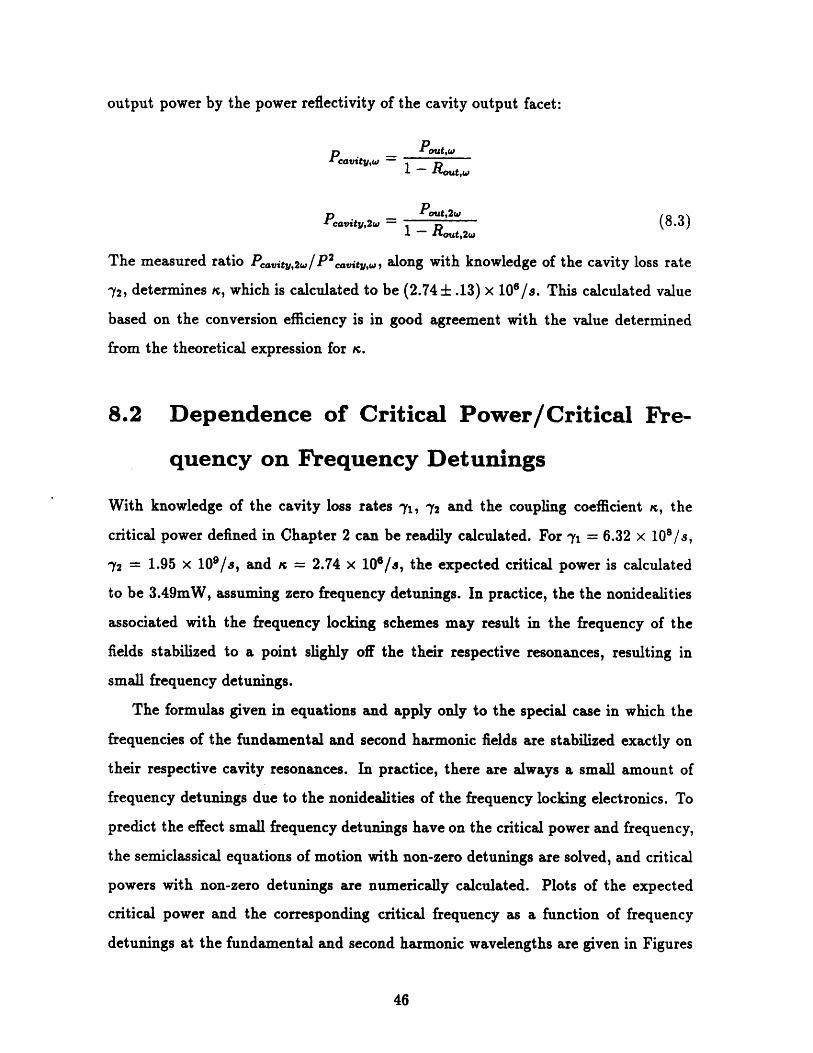
output power by the power reflectivity of the cavity output facet:
Pcvityw - t'.Pout,t,
Pcavity,2 - Pot,2, (83)1 - Rout,2w
The measured ratio Pc.aity,2w/P2cavity,w, along with knowledge of the cavity loss rate
72, determines K, which is calculated to be (2.74 ±.13) x 106 /s. This calculated value
based on the conversion efficiency is in good agreement with the value determined
from the theoretical expression for .
8.2 Dependence of Critical Power/Critical Fre-
quency on Frequency Detunings
With knowledge of the cavity loss rates -7, 2 and the coupling coefficient ar, the
critical power defined in Chapter 2 can be readily calculated. For 71 = 6.32 x 10⁸/s,
72 = 1.95 x 10⁹/s, and = 2.74 x 10⁶/s, the expected critical power is calculated
to be 3.49mW, assuming zero frequency detunings. In practice, the the nonidealities
associated with the frequency locking schemes may result in the frequency of the
fields stabilized to a point slighly off the their respective resonances, resulting in
small frequency detunings.
The formulas given in equations and apply only to the special case in which the
frequencies of the fundamental and second harmonic fields are stabilized exactly on
their respective cavity resonances. In practice, there are always a small amount of
frequency detunings due to the nonidealities of the frequency locking electronics. To
predict the effect small frequency detunings have on the critical power and frequency,
the semiclassical equations of motion with non-zero detunings are solved, and critical
powers with non-zero detunings are numerically calculated. Plots of the expected
critical power and the corresponding critical frequency as a function of frequency
detunings at the fundamental and second harmonic wavelengths are given in Figures
46

23a and 23b, respectively. Figures 24a and 24b give the same plots, except that
zero detunings are assumed in the fundamental mode. For detunings of '17, the
upper limit for this experimental setup, the critical power increases only slightly, to
3.55mW. Therefore, the amount of frequency detunings present in the experiment is
not expected to cause a significant shift in the critical power and critical frequency
from the nondetuned values. Appendix 4 details the derivations for the critical power
and frequency for zero detunings and the algorithm for numerically solving for the
critical power and frequency with non-zero frequency detunings.
8.3 Experimental Determination of Critical Power
From the discussion in Chapter 2, the critical pump power is the power level above
which self-pulsing oscillations take place and the linearized analysis from which the
intensity fluctuation spectrums are derived no longer applies. Also, the amount of
achievable squeezing improves as the input power is increased until the critical power
level is reached. Hence, the input power for optimum squeezing is one just under the
critical power level. From the previous section, a calculation of the input power level
yields 3.49mW with zero detunings. This power level is certainly within the capability
of the diode laser in use, which is capable of delivering approximately 20mW of
input power to the cavity. Experimentally, one looks for the critical power by raising
the input power until evidence of oscillation is detected. In this experiement the
photodetector output of either the reflected field or the transmitted field is displayed
on a spectrum analyzer. One then looks for oscillations in the frequency range within
which the critical oscillation frequency is predicted to lie. The experimental setups are
identical to the setups for noise detection (Chapter 7) and are shown in Figure 16. No
evidence of oscillation has been observed in either the reflected field or the transmitted
field spectrum for input powers up to 20mW. For the reflected field, where the large
amounts of optical power available provide a more promising setting for detecting
any oscillations, the enormous excess noise has probably swamped out any evidence
of oscillations. For the transmitted field, the limited optical power makes it likely
47
that any oscillations would be dwarfed under the presence of other noise sources, i.e.
thermal noise, amplifier noise, and frequency partition noise.
An attempt was made to reduce the excess noise from the reflected field by reduc-
ing the linewidth of the semiconductor laser via optical feedback. Two schemes shown
in Figures 25a and 25b have been attempted. In the first a small portion of the laser
output is diverted by a beam splitter onto a mirror. The mirror is adjusted to reflect
the beam directly back into the laser. In the second scheme a confocal Fabry-Perot
cavity instead of a mirror is used[12] [3] [13]. As shown in Figure 25b, the Fabry-Perot
cavity is aligned off axis such that the reflected field amplitude is maximized at the
resonance frequency of the Fabry-Perot cavity. Both schemes result in a reduction
of the laser linewidth. The first scheme also results in a reduction of approximately
10dB in the excess noise power of the reflected field for frequencies up to 50MHz.
However, the excess noise actually increases for higher frequencies. Since the critical
oscillation frequency is predicted to be around 400MHz, the slight reduction in excess
noise power below a frequency of 50MHz is not expected to increase the likelihood
of observing the critical oscillation. Experimentally, no evidence of oscillation was
observed with the linewidth reduction schemes.
48

Chapter 9
Detection Of Amplitude
Squeezing
In this chapter the amount of achievable squeezing for the KNbO 3 monolithic cavity
is discussed. The amount of achievable squeezing is based on the cavity parame-
ters measured experimentally. From Chapter 2 the intensity fluctuation spectrum
is expressed as a function of meausurement frequency and plotted in Figure 26a
using the experimentally determined parameters 71, 72, and . The plot assumes
that the input power to the cavity is at the critical power of 3.49mW. According
to Figure 27a, optimum squeezing occurs for measurement frequencies between 500
and 700MHz. A 31% reduction in intensity fluctuations below shot noise is predicted
for the fundamental mode at a measurement frequency of 590MHz. For the second
harmonic mode the best squeezing is achieved for measurement frequencies under
400MHz, where reduction in the intensity fluctuation of as much as 79% is predicted.
The intensity fluctuation spectrums for input powers at 10% and 1% of the critical
power are plotted in Figures 26b and 26c, respectively. At the lower input powers
the amount of squeezing is reduced at both the fundamental and second harmonic
wavelengths. As seen from Figures 26b and 26c, the frequencies at which optimum
squeezing is obtained are also reduced as the input power is decreased. At sufficiently
low input power, the best squeezing is achieved at dc for both wavelengths. Further
decrease in the input power results in reduction in the squeezing "bandwidth". That
49
is, the frequency above which the intensity fluctuation asymptotically approaches the
shot-noise level. Figure 27a and 27b show the squeezing spectrum as a function of
input power for fixed measurement frequencies. At the second harmonic wavelength
(Figure 27a), the amount of squeezing decreases monotonically with increasing input
power. At the fundamental wavelength (Figure 27b), however, the amount of achiev-
able squeezing has a maximum. The location of the maximum is a function of the
measurement frequency. Figure 28 shows a plot of the frequency at which squeezing
is maximized as a function of input power. The results obtained are self-consitent
with the conclusions derived from Figures 26b and 26c. Shown in Figure 27c is a
plot of the amount of achievable squeezing as a function of input power, regardless of
measurement frequencies. At the second harmonic wavelength, the achievalbe squeez-
ing scales inversely with input power. At the fundamental wavelength, the amount of
achievable squeezing is largely insensitive to input power. From the above calculations
one can conclude that to optimize the amount of squeezing at the second harmonic
wavelength, it is imperative to set the input power close to the critical power. At the
fundamental wavelength, the input power level is not a crucial experimental param-
eter as far as achieving optimum squeezing is concerned. However, for other reasons
such as noise performance discussed in Chapter 7, it is generally desirable to operate
at an input power close to the critical power.
The enormous frequency partition noise present in the output fields of the cavity
renders it impossible to detect amplitude squeezing using the the current setup. As
discussed in Chapter 7 the frequency partition noise arises from the imbalance in
the noise distribution between the main mode and the longitudinal sidemodes of the
semiconductor laser. One of the possible future modifications to the current setup is
to replace the semiconductor laser with a "quieter" laser source, such as a titanium
sapphire laser.
50

Chapter 10
Conclusion
An experimental setup aimed at generating squeezed light via second harmonic gen-
eration from a monolithic potassium niobate cavity was constructed. Active stabi-
lization of both the fundamental and second harmonic frequencies to their respective
cavity resonance frequencies was successfully implemented. The cavity loss parame-
ters Y1, 72, at the fundamental and second harmonic, and the nonlinear conversion
constant were determined from measurements of the bandwidth of the cavity at
the two frequencies and the conversion efficiency to the second harmonic. From the
cavity parameters the critical power and frequency can be calculated and used to
predict the achievable amount of amplitude squeezing as functions of measurement
frequency and input power. Table 3 provides a summary of the experimental results
obtained in this work. The results show that from the cavity design one expects to
observe significant amplitude squeezing at both wavelengths.
Expressions for the critical power and frequency as a function of cavity detunings
were derived. These results do not appear in the literature but are important for
relating theory to actual experimental conditions.
51
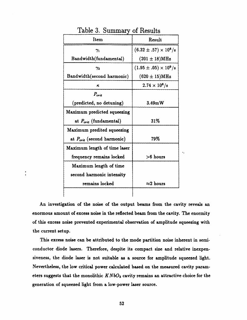
Table 3. Summary of ResultsItem
71
Bandwidth(fundamental)
72
Bandwidth(second harmonic)
Pcit
(predicted, no detuning)
Maximum predicted squeezing
at Pit (fundamental)
Maximum predited squeezing
at Pit (second harmonic)
Maximum length of time laser
frequency remains locked
Maximum length of time
second harmonic intensity
remains locked
Result
(6.32 : .57) x 108 /s
(201 ± 18)MHz
(1.95 ± .05) x 109/s
(620 ± 15)MHz
2.74 x 10⁶ /s
3.49mW
31%
79%
>6 hours
,2 hours
An investigation of the noise of the output beams from the cavity reveals an
enormous amount of excess noise in the reflected beam from the cavity. The enormity
of this excess noise prevented experimental observation of amplitude squeezing with
the current setup.
This excess noise can be attributed to the mode partition noise inherent in semi-
conductor diode lasers. Therefore, despite its compact size and relative inexpen-
siveness, the diode laser is not suitable as a source for amplitude squeezed light.
Nevertheless, the low critical power calculated based on the measured cavity param-
eters suggests that the monolithic KNbO 3 cavity remains an attractive choice for the
generation of squeezed light from a low-power laser source.
52

Bibliography
[1] J. C. Baumert, J. Hoffnagle, and P. Gunter. Nonlinear optical effects in KNbO 3
crystals at Al=Gal_.As, dye, ruby, and Nd:YAG laser wavelengths. In SPIE
Volume 492 ECOOSA '84, Amsterdam, the Netherlands, 1984.
[2] G. C. Bjorklund and M. D. Levenson. Frequency modulation (fin) spectroscopy.
Applied Physics B, 32:145, 1983.
[3] B. Dahmani, L. Hollberg, and R. Drullinger. Frequency stabilization of semicon-
ductor lasers by resonant optical feedback. Journal of Optical Society of America
B, 12:876, 1987.
[4] T. Debuisschert, S. Reynaud, A. Heidmann, E. Giacobino, and C. Fabre. Obser-
vation of large quantum noise reduction using an optical parametric oscillator.
Quantum Optics, 1:3, 1989.
[5] P. D. Drummond, K. J. McNeil, and D. F. Walls. Non-equilibrium transitions in
sub/second harmonic generation. 1. semiclassical theory. Optica Acta, 27(3):321,
1980.
[6] H. A. Haus. Waves and Fields in Optoelectronics. Prentice-Hall, Inc., Englewood
Cliffs, N.J., 1984.
[7] A. Heidmann, R. J. Horowicz, S. Reynaud, E. Giacobino, and C. Fabre. Obser-
vation of quantum noise reduction on twin laser beams. Physical Review Letters,
59(22):2555, 1987.
53
[8] C. H. Henry, P. S. Henry, and M. Lax. Partition fluctuatios in nearly single-
longitudinal-mode lasers. Journal of Lightwave Technology, LT-2(3):209, 1984.
[9] D. Hills and J. L. Hall. Response of a fabry-perot cavity to phase modulated
light. Rev. Sci. Instrum., 58(8):1406, 1987.
[10] R. J. Horowicz. Quantum correlation between fundamental and second harmonic
in shg. Europhysics Letters, 10(6):537, 1989.
[11] P. Kiirtz, R. Paschotta, K. Fielder, A. Sizmann, G. Leuchs, and J. Miynek.
Squeezing by second harmonic generation in a monolithic resonator. Applied
Physics B, 55:216, 1992.
[12] W. D. Lee and J. C. Campbell. Frequency stabilization of an external-cavity
diode laser. Applied Physics Letters, 57(21):2181, 1990.
[13] H. Li and H. R. Telle. Efficient frequency noise reduction of gaalas semiconductor
lasers by optical feedback from an external high-finesse resonator. IEEE Journal
of Quantum Electronics, 25(3):257, 1989.
[14] S. Machida, Y. Yamamoto, and Y. Itaya. Observation of amplitude squeezing in
a constant-current-driven semiconductor laser. Physical Review Letters, 58:1000,
1987.
[15] M. W. Maeda, P. Kumar, and J. H. Shapiro. Observation of squeezed noise
produced by four-wave mixing in sodium vapor. Optics Letters, 12(3):161, 1987.
[16] J. Mertz, A. Heidmann, C. Fabre, E. Giacobinao, and S. Reynaud. Observation of
high intensity sub-poissonian light using an optical parametric oscillator. Physical
Review Letters, 64(24):2897, 1990.
[17] C.D. Nabors and R.M. Shelby. Two-color squeezing and sub-shot noise signal
recovery in doubly resonant optical parametric oscillators. Physical Review A,
42(1):556, 1990.
54
[18] S.F. Pereira, M. Xiao, H.J. Kimble, and J.L. Hall. Generation of squeezed light
by intracavity frequency doubling. Physical Review A, 38(9):4931, 1988.
[19] K. Petermann. Laser Diode Modulation and Noise. Kluwer Academic Publishers,
Boston, 1988.
[20] R. V. Pound. Rev. Sci. Instrum., 17:490, 1946.
[21] M. G. Raizen, L. A. Orozco, M. Xiao, T. L. Boyd, and H. J. Kimble. Squeezed-
states generation by the normal modes of a coupled system. Physical Review
Letters, 59(2):198, 1987.
[22] E. A. Saleh and M. C. Teich. Can the channel capacity of a light-wave com-
munications system be increased by the use of photon-number-squeezed light?
Physical Review Letters, 58:2656, 1987.
[23] R. M. Shelby, M. D. Levenson, S. H. Perlmutter, R. G. DeVoe, and D. F. Walls.
Broad-band parametric deamplification of quantum noise in an optical fiber.
Physical Review Letters, 57(6):691, 1986.
[24] A. Sizmann, R.J. Horowicz, G. Wagner, G. Leuchs, and J. Miynek. Observation
of amplitude squeezing of the up-converted mode in second harmonic generation.
Optics Communications, 80(2):138, 1990.
[25] R. E. Slusher, P. Grangier, A. LaPorta, B. Yurke, and M. J. Potasek. Pulsed
squeezed light. Physical Review Letters, 59(22):2566, 1987.
[26] R. E. Slusher, L. W. Hollberg, B. Yurke, J. C. Mertz, and J. F. Valley. Ob-
servation of squeezed states generated by four-wave mixing in an optical cavity.
Physical Review Letters, 55(22):2409, 1985.
[27] P. R. Tapster, J. G. Rarity, and J. S. Satchell. Use of parametric down-conversion
to generate sub-poissonian light. Physical Review A, 37(8):2963, 1988.
[28] M. C. Teich and E. A. Saleh. Squeezed and anibunched light. Physics Today,
6:26, 1990.
55
[29] L. A. Wu, H. J. Kimble, J. L. Hall, and H. Wu. Generation of squeezed states
by parametric down conversion. Physical Review Letters, 57(20):2520, 1986.
[30] L.A. Wu, M. Xiao, and H.J. Kimble. Squeezed states of light from an optical
parametric oscillator. Journal of Optical Society of America B, 4(10):1465, 1987.
[31] A. Yariv. Quantum Electronics. John Wiley and Sons, New York, 1989.
56

Appendix A
I. Derivation of Expression For Cavity Loss Rate ?
The derivation below largely follows that given in Yariv's text[31, p. 147]. Consider
the intensity I of an optical beam. Let If denote the intensity after one roundtrip
through the cavity:
If = R1R2e-2alIi = e-2(-ln )Ii (.1)
Recall from Chapter 7 that a is the distributed loss per unit length; R1, R2 are the
mirror reflectivities of the input and output facets, respectively; and I is the cavity
length.
If one defines the loss per pass (as opposed to the loss per roundtrip) of the beam
to be L, such that
L = 1 e- e(a l- lnRR2) (.2)
the power loss per unit time of the beam is L x where n is the index of the medium.
The cavity loss rate y defined in (5.1) can also be defined by
dI = -27I (.3)dt
since intensity is proportional to the square of the field. Hence, the power loss per
unit time isc
27 = L (.4)nl
Substituting (.2) into (.4), one obtains
= C [1- e-(l'-'"n)] (.5)
57

For the case of L << 1,
-(1 -al + In R1Rt)= cal-InRR
Under this approximation,
c
in-
(.6)
(.7)11 R
-- InVRR 2)T
which is identical to (5.2)
II. Relating y to the Cavity Bandwidth AvFwHM
The Q-factor of the resonator is defined as
w£ wEP d£/dt (.8)
Here refers to the stored energy, and P refers to the dissipated power. Since the
energy inside the resonator is proportional to its intensity,
gEld/dtI 1
= I =d~lldt 2-f
One thus obtains,w27
The full-width-at-half-maximum bandwidth AvFWHM is given in terms of Q as
(.9)
(.10)
One gets, from (.11),
which is identical to (5.3)
58
AVFWHM = V/Q = (.11)
7 = 7rAIvFWHM (.12)

Appendix B
Estimation of Mode Partition Noise
Following the treatment used in Henry et. al.[8], a linearized model is used to
estimate the amount of excess noise power at the spectrum analyzer, following de-
tection of the reflected laser light from the cavity. The calculation assumes a modest
input optical power of 1.6mW and mode intensity fluctuation levels typical of diode
lasers. For simplicity one assumes that only two modes-the main mode and the first
sidemode-of the diode laser contribute to the mode partition noise.
The intensities of the two modes are denoted as follows:
I(t) = Io + AI(t)
J(t) = Jo + AJ(t) (.13)
I(t), J(t) are the intensities of the main mode and side mode, respectively, and
AI(t), AJ(t) are the intensity fluctuations in each mode. In the following analysis
it is also assumed that Io J and Io > AI,AJ. Henry et. al.[8] showed that
AI(t) = -AJ(t) using the simplified model. This requires that the total output
power is a constant in time:
I(t) + J(t) = Io + J (.14)
The above conclusion is not true, strictly speaking, since it does not account for the
the excess noise associated with the total laser output (RIN) observed experimentally.
However, since the excess noise of each mode far exceeds that of the total laser
output for typical diode lasers, the assumption of a constant total power is considered
reasonable.
The monolithic KNbO 3 cavity serves as a frequency selective filter. When the laser
59

is locked on resonance, the sidemode power is assumed to be completely reflected, but
only a fraction of the incident main mode power is reflected. The ratio of the reflected
power to the incident power is measured to be .72. The reflected power from the cavity
can thus be expressed as
Preflcted = .72I + J = .72(Io + AI) + (Jo + AJ)
Using the assumption AJ = -AI, one gets
Preflectd = (.72I + Jo) - .28AI (.15)
The reflected power thus contains a fluctuating term that is proportional to the
intensity fluctuation of the main mode only. The excess noise power of the reflected
field is thus
Poie,,op = .28AI (.16)
Referring to the noise detection scheme given in Figure 17, the fluctuation in the
intensity of the reflected field is detected by a photodetector, amplified by an rf-
coupled amplifier, and displayed on the spectrum analyzer. The noise power measured
at the spectrum analyzer can be expressed as follows:
Proiae,electl/AB = 42 B (.28)[r.pA] 2RiiGp (.17)
Here r,,,p is the responsivity of the photodetector; R, is the input impedance of
the rf-coupled amplifier; Gp is the power gain of the rf amplifier; and AB is the
measurement bandwidth of the spectrum analyzer. The fractional intensity fluctuaion
of the lasing mode is on the order of 10- for an input optical power of 1.6 mW. Thatis, ~ .~10 - 3. Using this value for 'x
is, 10- Using this value for we obtain an estimate for the excess noise
power at the spectrum analyzer and compare it to the value measured experimentally.
For an input optical power of 1.6 mW, AI = 16tW. Given that r,,.p = .613 A/W,
R, = 501, Gp = 57 dB, and AB = 741 kHz, the noise power is calculated from (.16)
to be -86 dBm/Hz. This estimated noise power is compared to the measured noise
60

power of approximately -85 dBm/Hz given in Figure 20. According to the presently
used model, as the input optical power increases, the power fluctuation is correspond-
ingly increased, giving rise to enhanced excess noise at higher photocurrents. This
behavior is not observed experimentally. As shown in Figure 20, the excess noise
power saturates to approximately -80 dBm/Hz for for photocurrent levels above 1
mA.
From the above calculations one finds that to within an order of magnitude the
estimated excess noise power agrees with the measured excess noise power for an
input optical power of 1.6 mW. The calculated result shows that mode partition
fluctuations do indeed produce enormous excess noise power when the laser output
field is filtered.
61
Appendix C
Determining K From Amount of Second Harmonic Conversion
We first derivee a relationship between the normalized field variable a and the
physical power P.
The intensity of a plane wave propagating in a medium of index n is
E2
I =< S > 2, (.18)
where E is the electric field, and v = F is the characteristic impedance. Since the
index n is related to the permittivity e by e = n2 Ce, (.18) can be expressed as
I =< S >= -cne0lE12 (.19)2
From (2.10) the electric field £ is related to the normalized field amplitude a by
2g 1Substituting (2.10) into (.19), one obtains
cnhwI = -- lal2 (.20)
The power, obtained by integrating over the area of the beam, is given in terms of
the normalized field variable a as
P = cnhl,2 (.21)1
The power P derived above denotes the circulating power inside the cavity, and I is
the cavity length.
62

In the steady state, the time derivatives in the equations of motion given in (2.9)
vanish. That is, ddal = = . Assuming further that there are no frequency
detunings, A = 2 = 0, r; can be expressed as a function of the normalized field
variables:
K = 2Y2 (.22)a1 0
Here alo and a20 denote the steady-state normalized field amplitudes at the funda-
mental and second harmonic frequencies, respectively. By expressing clol and la 20o
in terms of physical powers using (.21), (.22) becomes
2cnhlwlPcavity,2w (.23t~ = 2 (.23)
IP cavity,w
where Pcavity,w and Pcavity,2w denote the optical power inside the cavity at the funda-
mental and second harmonic wavelengths, respectively.
63

Appendix D
I. Derivation of Expression For Critical Power With No Frequency
Detunings
From the equations of motion given in (2.9), expressions for small perturbations
6al, 6a2 around steady state values a10 and a20 can be obtained (with the additional
assumption of zero frequency detunings A1, A 2):
dd6al = -7 16al + Ka20oal1 + Kaclo6a2dt
d~fal = Ka2o*fal - 716al1 + cKalOc6a2*
didc a2 = -Caloal - 72 a2 )
dtd 6a2' = -Calo* - 72Ea2' (.24)
Assume Sal, 6a 2 oc et, where A are the eigenvalues of the 4th-order matrix given
above. Solving for the eigenvalues, one obtains
]\1, 2- [-KCa2 01 + 71 + 72] [(-I 201 + I - 72)2 - 4alo2]
34 = - -a 2o0 + 7 + 721 ± [(a 20 + 71 -2) - 4Kalo2]2 (.25)
These eigenvalues are used to determine the stability of the solutions.
Under the conditions of steady state and zero frequency detunings:
dar cao*a 20 + 1= 0 = -7'a 0Ylo + r-l 2 + dt
da 2z 1a2 = 0 = -2a2o- alo 2 (.26)dt 2
64

Rearranging, one gets
61 = 7110 - alo0*a20 (.27)
2 2a1 0o -- 2020 (.28)
Multiplying (.27) by its own complex conjugate and then substituting (.28) into re-
sulting expression, one obtains, after some algebraic manupulation, an expression
relating the second harmonic field amplitude to the input pump power:
Ies 12 = -272 (Ka20) 3 + 47172 (a 2 0)2 - 2 272 (na 20) (.29)
The expressions for Al, A2 become, upon substituting (.28) into (.25),
A1, A2 = -[-Kla 2 0o + sy + 12] i [±[Ia2012 + (1 - 2)2 - 2lIa2ol(yl + 3y2)]2 (.30)For small, 2 small. In this regime A, contain negative real parts, and
For El small, Kra20o is small. In this regime A1, A2 contain negative real parts, and
the solution of a 2 converges to a20 as t -== oo. As ta20 == -(-1 + 72), the negative
real parts of A1, A2 vanish, leaving purely imaginary parts:
A1 ,A2 = +i[Y2(2- 1 + 2)]½2 (.31)
The magnitude of the purely imaginary parts of A1, A2 is the critical oscillation
frequency:
crit, = /( + '2) (.32)
The pump power at which A1, A2 become purely imaginary is the critical pump power.
Subsituting Ka20 = -(,1Y + 2) into (.29), one gets
IElc12 = 272(71 + 72)(271 + 72)2 (.33)
Taking the square root and dividing by K, one obtains the expression for the critical
65

pump power in terms of 71, 72, and :
Ificl = IC FY272(71+72) (.34)
II. Algorithm for Determining Critical Power and Frequency With
Nonzero Frequency Detunings
The linearized equations around the steady state solutions a1 0 , a 2 0 with nonzero
frequency detunings are
6al = -(71 + iA 1)6al + Ka20oal* + lo*10Sa20
al* = -(71 - iAl)al* + Ka20*6al + Csal0 a2*
fa2 = -(72 + iA2 )6a2 - Kcal06al
5a2' =-(72 - i 2)6a2' - al06al (.35)
The eigenvalues of this 4th-order matrix equation are given by the roots of the fol-
lowing 4th order polynomial:
A4 + [2(71 + 7 2)]A3 + [(722 + 22 ) + 47172 + (712 + A12 ) + 21ralol 2 - IKa2 ol]2 A2
+[27(722 + A22) + 272(712 + A1
2) + 21alo 2(7l + 72) - 21Ka2o1272]A
+ (712 + A12 )(7 2
2 + A2 ) + 21Ca1ol2(7l7 2 - A1 A2) - Ka2012(722 + A2
2 ) + Ialol4 (.36)
Again, by assuming steady state, one can set the time derivates equal to zero in the
equations of motion and obtain the following expression for alo and el:
2a10o -- (72 + iA 2)a2o (.37)
el = (71 + iAl)aio + ca10o'a 20 (.38)
66
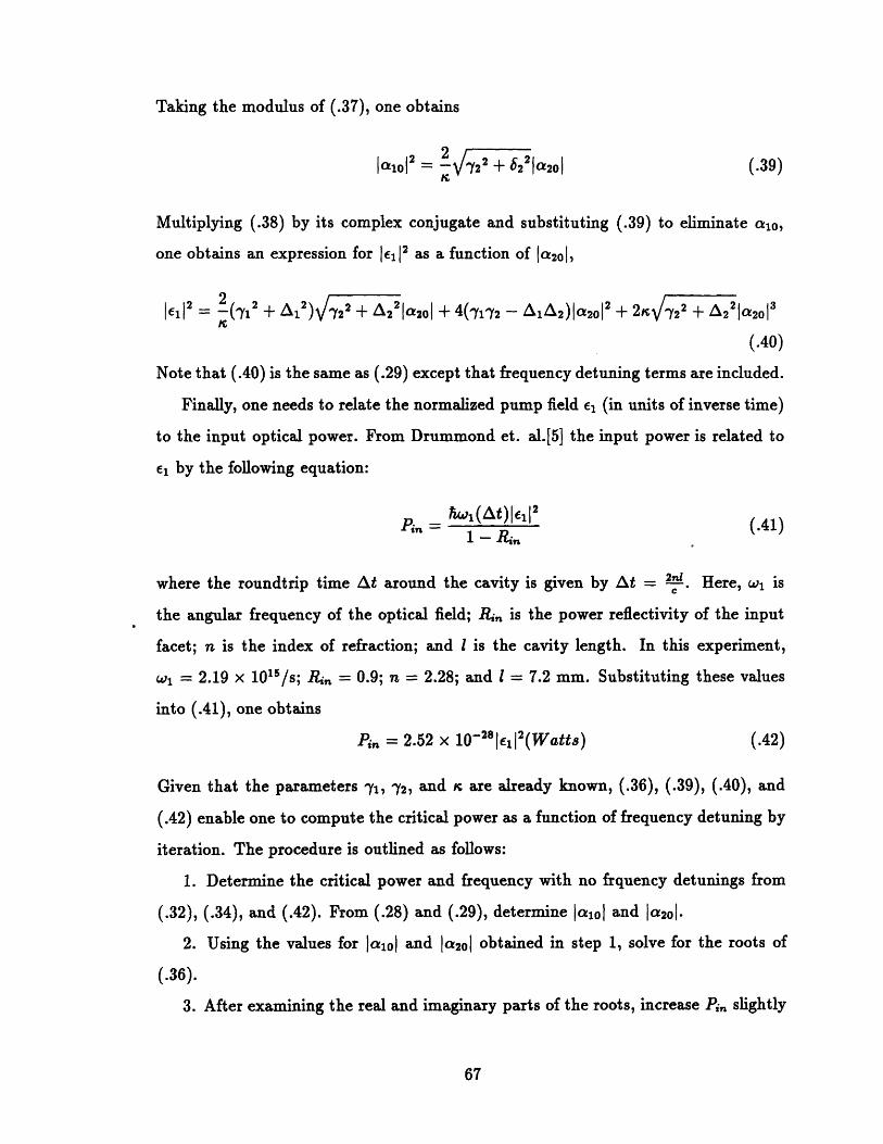
Taking the modulus of (.37), one obtains
l 1J02 = 2 722 + 6221a 201 (.39)K
Multiplying (.38) by its complex conjugate and substituting (.39) to eliminate ao0,
one obtains an expression for 1 112 as a function of a20 1,
EI1 =- 2_ ( + A1 )722 + 22 1a2o01 + 4(7172- AA 2)la 2 01 + 2JV722 + Al22 a2o01
(.40)
Note that (.40) is the same as (.29) except that frequency detuning terms are included.
Finally, one needs to relate the normalized pump field 1 (in units of inverse time)
to the input optical power. From Drummond et. al.[5] the input power is related to
i1 by the following equation:
Pi, = iw(t) l 12 (.41)1 -Rn
where the roundtrip time At around the cavity is given by At = 2'. Here, w is
the angular frequency of the optical field; RP, is the power reflectivity of the input
facet; n is the index of refraction; and is the cavity length. In this experiment,
wl = 2.19 x 10¹⁵/s; Ri, = 0.9; n = 2.28; and I = 7.2 mm. Substituting these values
into (.41), one obtains
Pin = 2.52 x 10- 281l 112(Watts) (.42)
Given that the parameters 71, 72, and are already known, (.36), (.39), (.40), and
(.42) enable one to compute the critical power as a function of frequency detuning by
iteration. The procedure is outlined as follows:
1. Determine the critical power and frequency with no frquency detunings from
(.32), (.34), and (.42). From (.28) and (.29), determine Jlalo and a2o01
2. Using the values for alol and Ia2o0 obtained in step 1, solve for the roots of
(.36).
3. After examining the real and imaginary parts of the roots, increase Pin slightly
67

from the critical power with no frequency detunings. Recalculate ailol and a 20o and
solve for the roots of (.36) again to obtain a new set of roots (eigenvalues). Continue
the iteration process until the real part of one of the conjugate pairs of roots vanish.
The value of Pin for which this condition is satisfied is the new critical power. The
imaginary part of the roots becomes the new critical frequency.
68

a) Four Wave Mim,,
c (output)
W3 (input)
(pump)
l(pum
(02(pum)
b) Optical Parametric AmpliflcationOcillation
o3 (input)
C) Second Haruonic Generation
(OlitEUt) 2. (ineut)
(OUtDUt)o
Figure 1. Three processes from which squeezing has been generated.
n (t)n
-n (:k,) -n (-A,)
A.
Figure 2. Dependence of index of refraction on wavelength for an anisotropic medium.
69
(output) co(OUtUUt-~ 3
J

R=90% @ 860nmR=97.5% @430nm
Ca
a
to high voltage source
electrode
F
incident/reflected)
R=99.85% @860nmR=98.4% @430nm
(transmitted blue)
(transmitted red)
/1/1crystal dimensions: 7mm x 3mm x 3mm
Figure 3. Doubly resonant monolithic cavity for second harmonic generation.
n2.2770
n(second harmonic)
n(e)=2.2768
2.2766
n(fundamental)
29
T(degrees C)
Figure 4. Phasematching by temperature and by electro-optic effect.
70
I
-
Il
--_v

9D
94093092091090890880870860850840ao0
-40-20 2020 0 60 80 00120 14010 0 200
Temperolure (c)Figure 5. Temperature dependence of the phasematching wavelength for the nonlinear
optical coefficient d32 of KNbO 3.
71
EC
C0
0
c
-
CL
A m , -

bias T network
plate
Figure 6. Experimental setup.
72
filter
isolator
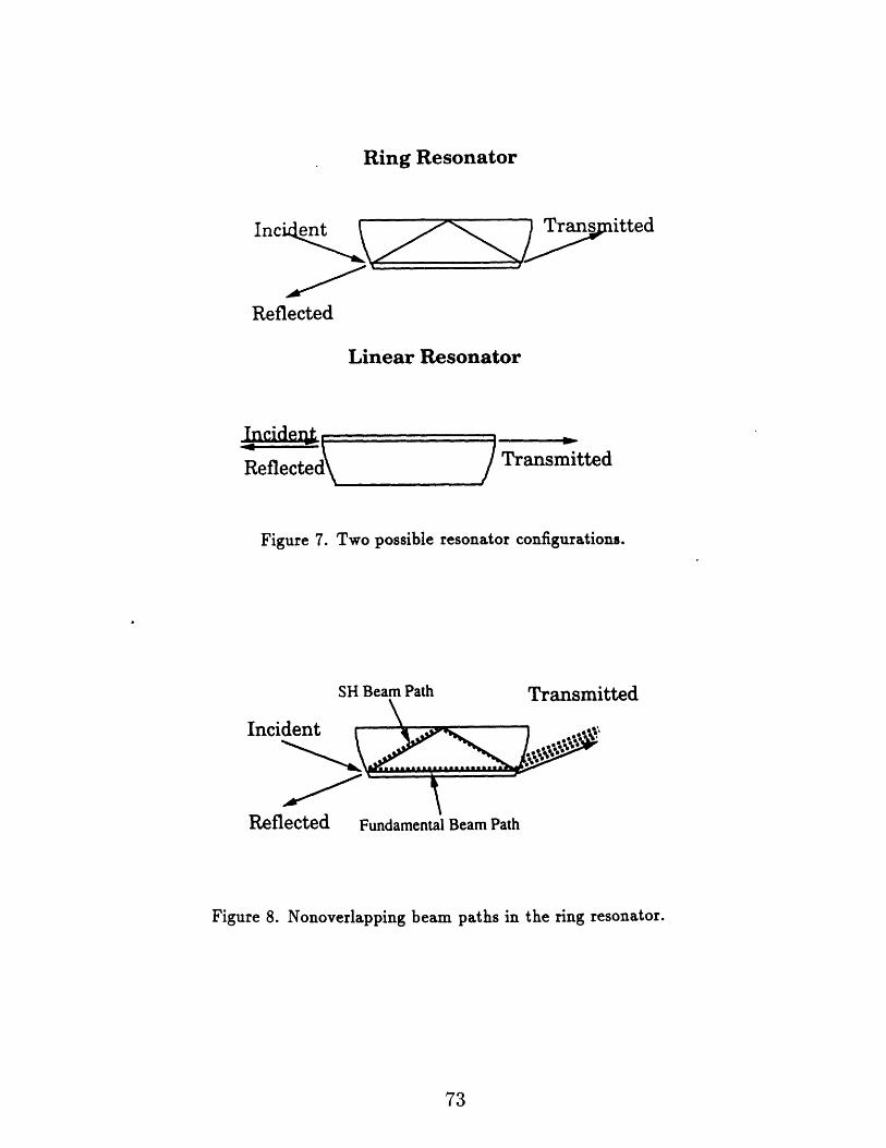
Ring Resonator
Inc ent Transitted
Reflected
Linear Resonator
Tn rifnt
Reflected I Transmitted
Figure 7. Two possible resonator configurations.
SH Beam Path
Incident
Reflected Fundament;al Beam Path
Figure 8. Nonoverlapping beam paths in the ring resonator.
73
_ t L-- -&so. I ~
-
Tr·q nqrniff.Pti.^vv_
- -----------------

diode laser bias current ramp
Figure 9. Cavity transmission as a function of frequency detuning from cavity resonance.
Ca&ity transfer function:
I77
:t o- -
'_ i I
/ A, = ,(/ -f. x o = of -
x ArcoJ I 2. tt - Ain( 2 .,t2 l
Adjust suchthat 1., x A.
laser
Figure 10. Pound-Drever locking scheme.
74

100 nF
R
-15 V
Gain Stage Integrator Stage
Figure 11. Loop filter circuit.
I
Vo· LL _ - -- euLiLg
Figure 12. Error signal as a function of frequency detuning from cavitY e..
75

V = V: V CCst-t
Photo-detector
-. .,crPi. . --
*:.. _ : ' ..t..
:.~d O~ S,. - .
V = - Cos ,Case (v.>V
r It,\
V.- .V-V V
P.,
v
Pjc - pcs(2,Jt-+2)Ver-r - F..i&
Figure 13. Setup for locking the second harmonic output intensity.
76
| b
LM - s~~~
C:-, 4 f ( V ,- .el ,P 1 (v. . )o
I
i :, . I
I ;I.4. \ 1r tV-t
¢-¢ V~-,,
I'll.tXtVr' ~/.v~
P"' -P.+ P I- t+ P \
IV e- - P. , C- C

I
Low input power:negligible thermal effect
aput power:thermal effect
To TFigure 14. Temperature dependence of second harmonic intensity in the vincinity
of phasematching.
I
TATo
Figure 15. Hysteresis effect of second harmonic intensity as a function of temperature.
77
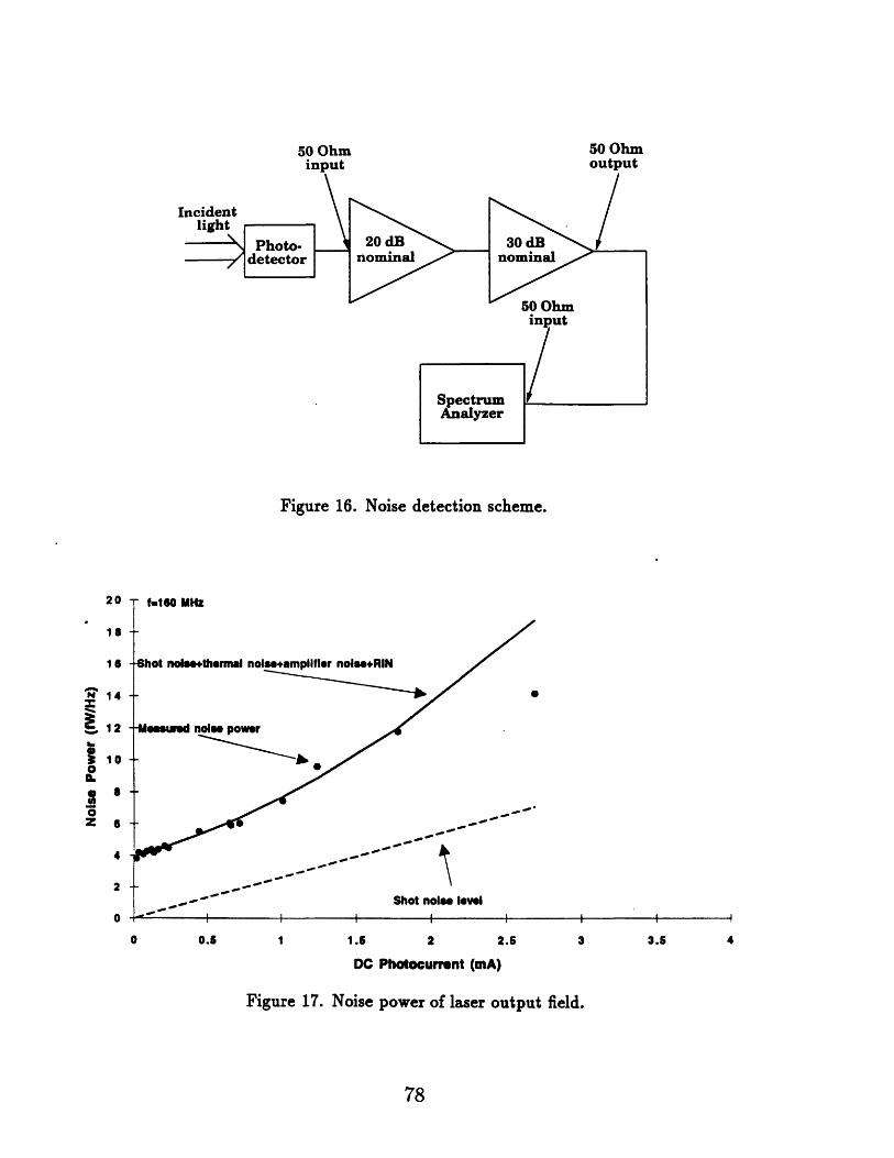
Ohm
I:
Analyzer
Figure 16. Noise detection scheme.
f-16O MHz
hot noledothermal nolse+ampllller nolu+RIN
lesusd no, power
0
- - --- - .-
- - - --
Shot nolse level
0 0.5 1 1.5 2 2.5 3
DC Photocurrent (mA)
Figure 17. Noise power of laser output field.
78
20
18
16
N 14
12
3 10
a'Z 6
2
0
3.5 4
_ m

40 0.5 1 1.5 2 2.5 3 3.5
DC Photocurrent (mA)
Figure 18. Noise power of laser output field following reflection from a mirror.
FncusingSw
mta
*usinglens
,lain mirror
Figure 19. Optical path of laser beam reflected from a plain mirror.
79
20
18
16
- 14N
12
I
o
4
2
0
_ _ _ _1

1 l1 0
N1=E-12
I-0
° 15-141E-13 a.Z
1E-15
1E-18
- f- 110 MIIZT* I DU MHz
A
Measured noise power
Power due to shot noise, thermal noise, and amplifler noalse
/// Shot noise level
-1 ' I I -I
0 0.5 1 1.5 2 2.5 3 3.5 4
DC Photocurrent (mA)
Figure 20. Noise power of reflected fundamental field.
f..mod- 198MHz Idcs 1.6 mA
Idc 0
I i OW I I I . f . I
0 0.1 0.2 0.3 0.4 0.5 0.6 0.7 0.8 0.9 1
Frequency (GHz)
Figure 21. Measured noise spectrum of reflected fundamental field. The detected
photocurrent is 1.6 mA (upper trace). The lower trace shows the noise spectrum
with the laser beam blocked from the photodetector.
80
U-
-10
-20
Ei -30.40
0C.
a -50
-70
-80
I I

' f- 10 MHz
Mosurned ols power
Power due to shot noise, thrm noise, and smpllftr noise
. . 2 2.6 3 3.5 4DC Photocurrent (uA)
power of transmitted second harmonic field.Figure 22. Noise
81
1E-1
1E-14
o 1E-lih.
Z 1E-15
1E-1711Ee16
oCr .I-l1
- - - - - - - - - - - - - - - - - - - - - - - -
Shot nise leve

· rmr1- i.-3286a /I
deltal f x gammal
delta_2= f x gamma_2
0 0.1 0.2 0.3 0.4 0.5 0.6 0.7 0.6 0.9
Frequency Detuning as a Fraction of Gamma (f)
Figure 23a. Critical power as a function of frequency detuning.
gamma_1- 6.320 /a
gamma_2. 1.95.9
kappa. 2.74.6 /I
delta. 1- x gammal
delta_2- f x gamma_2
0 0.1 0.2 0.3
Frequency
0.4
Detuning
0.5 0.6 0.7
As A Fraction of Gamma (f)
0.8 0.9 1
Figure 23b. Critical oscillation frequency as a function of frequency detuning.
82
12
10
E
o3a00.
UI-um. E
8
6
4
2
0
bUU
500 -
400
300
Nz
I.I.0cicu5rr.C.
200
100
0
.
_ r I I ! I & i I II W I
r-f-
t
I I I

1Z
1 0
E 8
Uo 6
o. 4
2
0
0 0.1 0.2 0.3 0.4 0.5 0.6 0.7 0.8 0.9 1
Frequency Detuning as a Fraction of Gamma (f)
Figure 24a. Critical power as a function of frequency detuning in the second harmonic
mode only.
bUU -
500 -
N
:K 400
cC0)c 300 -
IL
Z 200 -
OC. 100 -
0
gammal. 6.32.8 Isgamm_2- 1.959 a
kappa- 2.74M /
deltal- 0d elta_2 f x gamma_2
I I I I I
0 0.1 0.2 0.3 0.4 0.6 0.6 0.7 0.8 0.9 1
Frequency Detuning As A Fraction of Gamma (f)
Figure 24b. Critical oscillation frequency as a function of frequency detuning in the
second harmonic mode only.
83
4 l ......

HR
Plane mirror
/
Figure 25a. Laser linewidth reduction scheme. Optical feedback is provided by
plain mirror.
Cavity mirrors
To cavity
.Scanning FabryPerot Resonator
Figure 25b. Laser linewidth reduction scheme. Optical feedback is provided by
Fabry-Perot resonator.
84
kt

Cavity BandwidthT of Fundamental , Cavity
__I~~~~~~~~~~ ; ~~Pcrlt=3.5mWof Secou
Pin= Pcrlt I
1 I 1
Fundament
Bandwidthad Harmonic
al
Kappa-2.746/s I
Gamma_1- 6.32x10^8 /s
Gamma_2- 1.95x10^9 /sI
. i I I I I
300 400
Frequency (MHz)
500 600
Figure 26a. Squeezing spectrum for Pi, = Pcrit.
Pcrlt=3.5mW
Pin- Pcrlt/10
Kappa-2.74s6/s
Gammal- 6.32x10⁸ /Is
Gamma_2= 1.95x10^9 /a
Second Harmonic
0 100 200 300 400 500 600
Frequency (MHz)
Figure 26b. Squeezing spectrum for Pi, = Pit.
85
-
1
_ 0.9E
_- 0.8o.sa.u) 0.70,c 0.6a)4). 0.5Co/)' 0.4N
3 0.3E0Z 0.2
0.1
onc I J
0
0 100 200 700
1
0.9E
0.8C.)a)W0.7
0.6
U 0.5r 0.4
03- 0.2.1
aa 0.4
0.3
0
700
v
III I
III I -. 0
IF
1t

Pn~ PcriU100i 0
Second Harmonic Fundamental
+i~~~~~~~~~~ ~Kappa2746/i~~~~~~~~~~~~~~~~Kpa27e/Gamma_1. 6.32x10"8 /s
Gamma_2. 1.95x10"9 /a
200 300 400 500
Frequency (MHz)
Figure 26c. Squeezing spectrum for Pin = P.it-
Measurement freq- 20MHz
9mW
Kappa- 2.74x10^ /a
Gammal. 6.32x10⁸ /IsGamma_2- 1.95x10^9 /s
0.1 1
Input Power (mW)
Figure 27a. Power dependence of squeezing in the second harmonic mode at 20MHz.
86
T
o 0.9E3
C)0.5a', 0.7N 0.6N
o0.5Z 0.D 0.4N
'0 0.3
0
0.1
0
0 100 600 700
0.9
0.8
0.7
0.6
0.5
0.4
0.3
0.2
cU
N
Cnu0)
N
E0Z
0.1
0
0.01 10
- l~~~~~~~~~~~ ----- e--
. i
r
i
! 1t

9% squeezIngat Pcrit
23% queezIngat Polt
31% queezlng
Measurement fraq, 20 MHz
Kappa. 2.74x10^6 /
Gamma-l- 6.32X10A8 s
Gamma-_2 1.95x10^9 Is
0.1
at Pcrit
Measurement trean 380 MHz
1
Input Power (mW)
Figure 27b. Power dependence of squeezing in the fundamental mode at 20MHz, 380MHz,
and 590MHz.
Fundamental
Kappa= 2.74x10^6 Is
Gamma_l 6.32x10^IO I
Gamma_2- 1.95X10^9 /I
.U mW
(
Second Harmonic
0.O0 0.1 1 10
Input Power (mW)
Figure 27c. Power dependence of the maximum achievable squeezing in the fundamental
and second harmonic modes.
87
1
0.9
a 0.8
( 0.7
0)0 .6 -
Z 0.5-uT/)
0.4
0.3Z 0.2
0.1
0
0.01 10
1
. 0.9E
0.8
0.m) O.70)c
oZ- 0.2.1
o 0.5
0
0.1
0
I I I _ _
I i_
-- _ .. .. .
_
... _ _ _ _. . . . - _ o
I

Kappa- 2.74x10^6 /s
Gammal- 6.32x10A8 /s
Gamma_2- 1.95x10^9 /s
Fundamental
J1JV
Jle
.00
Second Harmonic
S - '
-.
00
/-
//
Input Power (mW)
Figure 28. Optimum measurement frequency for squeezing as a function of input power.
88
OUU
5
4
00
00
E
Ea0o
c
_ 3c v4) N0)C
E
0CO
300
2
1
00
00
S
0
0.01 0.1 1 10
A
G e.