Generating entanglement with linear optics

Stasja Stanisic,1, 2 Noah Linden,3 Ashley Montanaro,3 and Peter S. Turner1

1Quantum Engineering Technology Labs, H. H. Wills Physics Laboratory andDepartment of Electrical & Electronic Engineering, University of Bristol, UK

2Quantum Engineering Centre for Doctoral Training, University of Bristol, UK3School of Mathematics, University of Bristol, UK

(Dated: September 26, 2017)

Entanglement is the basic building block of linear optical quantum computation, and as suchunderstanding how to generate it in detail is of great importance for optical architectures. Weprove that Bell states cannot be generated using only 3 photons in the dual-rail encoding, and givestrong numerical evidence for the optimality of the existing 4 photon schemes. In a setup witha single photon in each input mode, we find a fundamental limit on the possible entanglementbetween a single mode Alice and arbitrary Bob. We investigate and compare other setups aimedat characterizing entanglement in settings more general than dual-rail encoding. The results drawattention to the trade-off between the entanglement a state has and the probability of postselectingthat state, which can give surprising constant bounds on entanglement even with increasing numbersof photons.

I. INTRODUCTION

Research into quantum technologies has gained signif-icant momentum in the last several years, with appli-cations ranging across metrology, communications, secu-rity, simulation and computation [1–4]. One of the im-portant resources lying behind many of these advancesis quantum entanglement [5, 6]. Long before it was apotential technological resource, entanglement was stud-ied as one of the phenomena lying at the foundations ofquantum mechanics [7–9]. That there exist non-classicalcorrelations between physical systems is now well estab-lished, while how best to generate, verify and quantifysuch entangled states in practice is an ongoing field ofactivity. What is practical in any given situation de-pends on the physical platform under consideration; herewe will be interested in the generation of entanglementusing linear optics and postselection.

In linear optics we study collections of optical modes,modelled as harmonic oscillators whose excitations cor-respond to photons. Interactions are restricted to Hamil-tonians that leave the total number of photons fixed,giving rise to unitary transformations on modes (inter-ferometers), as well as possible measurement and posts-election of quantum states (heralding). This realizationintroduces an interesting set of constraints on the en-tanglement problem. Most work to date focuses on ei-ther single- or dual-rail encoding of photons into two-dimensional qubits, and then applying the usual ap-proaches to quantum computation such as the circuitmodel or measurement-based schemes. Gates are car-ried out via ancilla modes and photon detection measure-ments [4]. The dual-rail encoding, where qubits are real-ized as single photons in pairs of spatial or polarizationmodes, is the commonly accepted standard for quantumcomputation with linear optics, and allows us to discussentanglement in terms of standard concepts such as Belland GHZ states [4, 10, 11]. However, the requirementof postselection means generation of such states is non-

deterministic, and the probability of success is often low;for example, the best known Bell state generation schemehas success probability of 1/4 [12] and if the postprocess-ing technique known as procrustean distillation is notallowed, then the probability drops to 0.1875 [13]. Whenwe consider the number of Bell states needed to constructtwo-dimensional cluster states [11], the requirements canbe quite daunting, though promising proposals exist [14].

This helps to motivate the study of entanglement gen-eration in linear optics more generally; in particular, it isnatural to consider entanglement between two subsets ofmodes, foregoing encoding altogether. While this is cur-rently not the preferred way of generating entanglement,any bounds that can be found present fundamental limitson linear optical architectures, as well as for other quan-tum information processing tasks such as boson sampling[15]. A different perspective on this issue, which consid-ers bosonic entanglement in terms of observables, can befound in (e.g.) [16, 17].

In this paper we will consider two main themes regard-ing bipartite entanglement in linear optics; that wherethe parts are encoded qubits, and that where they arecollections of modes. Section II introduces the back-ground and notation used throughout. Section III exam-ines qubit entanglement within the standard linear opti-cal dual-rail encoding. When we speak of dual-rail encod-ing, we mean qubit states that are post-selected such thatthere is exactly one photon in each pair of modes. Firstwe prove that one cannot generate a Bell state using only3 photons, and then we give strong numerical evidencefor the known 4 photon Bell state generator (with a suc-cess probability of 0.1875) being optimal. In Section IVwe compare qubit and mode entanglement, including aninvestigation of the expected average entanglement overuniformly (Haar) distributed interferometers. In SectionV we shift our focus to mode entanglement, consideringbipartite systems made from two sets of optical modes,Alice and Bob, with a fixed total number of photons. Wesee two types of behaviour. In the case of bunched photon

2

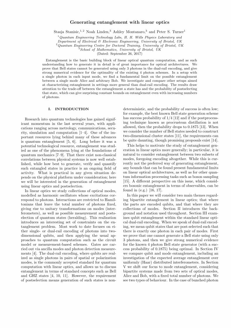
Bound (ebits) Parameters Input state Section

O(logn) MA = 1,MB = 1,MH = 0 Bunched V A 1

2 MA = 1,MB ≥ 1,MH = 0 Unbunched V A 2

log 3 MA = MB = 1,MH ≥ 1 Unbunched V A 3

log(

2(MA+n−1

2MA

))MA = MB , n odd Any V B 1

log(

2n+MAn

(MA+n2−1

MA

))MA = MB , n even Any V B 1

n MA = MB Fock state V B 2

TABLE I. Entanglement bounds proven in this paper. The notation is as defined in Section II (see Figure 1).

input and single mode Alice, we find the entanglementcan grow as log n where n is the number of photons. Onthe other hand, looking at the case of at most a singlephoton per input mode (as in, for example, boson sam-pling [15]), a single mode Alice and no measurement, theentanglement is bounded above by 2 ebits regardless ofhow many photons are present. If we also restrict Bobto a single mode and furnish the remaining modes withnumber resolving detectors, the expected entanglementis bounded by log 3 ebits. We then find provable uni-versal bounds on the mode entanglement stemming fromthe dimensionality of the bipartite Fock states involved,and from the linearity of the optical transformation. Fi-nally, we conjecture a third bound due to unitarity whichextends the previously mentioned constant bound in thecase of Alice having a single mode to multi-mode Alice,and we provide numerical evidence for this conjecture.The maximum mode entanglement is summarized in Ta-ble I.

II. BACKGROUND

......

......

...

MI

MV

MA

MB

MH

U

...

n1

FIG. 1. The generic setup used throughout this paper; seetext for an explanation of the notation.

Figure 1 introduces the generic linear optical setup andnotation used throughout the paper. The interferometerhas M input modes and M output modes. The mode

transformation describing this (photon number preserv-ing) interferometer is an M × M unitary matrix U ∈U(M). The top MI input modes contain n input pho-tons, while the bottom MV modes are ancilla vacua. Therepresentation of U carried by the n photon, M modeHilbert space in the number state (Fock) basis is de-noted U (n). The top MA output modes belong to oneparty, Alice, the middle MB modes belong to Bob, andthe bottom MH modes – Harold – get measured usingphoton counting detectors. Harold’s detection pattern islabelled h = (nMS+1, · · · , nM ) where ni gives the pho-ton number of output mode i, and MS = MA + MB isthe number of modes in the “system”, i.e. modes thatdo not belong to Harold and are therefore unmeasured.

If nH =∑Mk=MS+1

nk = ||h||1 total photons have been

detected, the number of photons left in the system isnS = n − nH = nA + nB . The Hilbert space of subsys-tem X (a subset of modes), given that it contains exactlynX photons, is denoted HnX

X .Let the input to the interferometer be a Fock state

|ψin〉 = |n1, n2, · · · , nMI, 0, · · · , 0︸ ︷︷ ︸

MV

〉 (1)

=

MI∏k=1

(a†k)nk

√nk!|vac〉 , (2)

where |vac〉 = |0〉⊗N . The input transforms according to

U |ψin〉 =

MI∏k=1

1√nk!

(U a†kU

†)nk

U |vac〉 (3)

=

MI∏k=1

1√nk!

M∑j=1

a†jUjk

nk

|vac〉 , (4)

where Ujk are the matrix elements of the mode transfor-mation U , U is the representation of U on the multimodeFock space, and we have used the fact that the vacuumis invariant under all such transformations (as is custom-ary, we have suppressed identity operators on ancillarymodes). We will usually be interested in the case of sin-gle photon Fock inputs, where nk = 1 or vacuum for allinput modes k, a situation we will refer to as unbunched.If all the photons are found in one mode and the restcontain vacuum, we will refer to the state as completelybunched.

3

When MH > 0 the ideal number resolving detectorswill register a detection pattern h = (nMS+1, · · · , nM ) ofnH photons. The output will be the post-measurementstate consisting of nS = n−nH photons remaining in thesystem modes 1, · · · ,MS , given by

|ψS(h, U)〉 =〈h|U|ψin〉‖ 〈h|U|ψin〉 ‖

. (5)

Note that this is a pure state on the system S = AB, be-cause |h〉 only has support on subsystem H. We will de-

note the unnormalized output by |ψS(h, U)〉 = 〈h|U|ψin〉.The Hilbert space of the system is

HnS

S =

nS⊕nA=0

HnA

A ⊗HnB

B , (6)

where nB = nS − nA is the number of photons in Bob’ssubsystem. We are interested in entanglement with re-spect to this tensor product structure. The dimension ofthe Hilbert space of n photons in M modes is

(M+n−1

n

),

and so

dimHnS

S =

nS∑nA=0

(MA + nA − 1

nA

)(MB + nB − 1

nB

)(7)

=

(MS + nS − 1

nS

)(8)

as MS = MA + MB and nS = nA + nB . The totality ofstates available to Alice can be thought of as the Hilbertspace

⊕nS

nA=0HnA

A , and we may index its Fock basis as

{|a〉A : a = (n1, n2, · · · , nMA), ||a||1 = nA}. Similarly

for Bob. Expanding the output in this basis, we have

|ψS(h, U)〉 =∑a,b

Ca,b(h, U) |a〉A ⊗ |b〉B . (9)

The coefficients C are related to permanents of the ma-trix U [15, 18]. More specifically, consider an inputFock state |ψ〉 = |n1 · · ·nM 〉 and an output Fock state|φ〉 = |n′1 · · ·n′M 〉 both with a total number of n photons.Construct a new matrix Uψφ from U in two steps. First,define the matrix Uψ consisting of nj copies of the j-thcolumn of U for all j ∈ {1, · · · ,M}. Next, construct thematrix Uψφ by using n′j copies of the j-th row of Uψ forall j ∈ {1, · · · ,M}. Then

〈φ| U |ψ〉 =perm(Uψφ)√

n1! · · ·nM !n′1! · · ·n′M !. (10)

In our notation, |ψ〉 = |ψin〉 and |φ〉 = |abh〉, we there-

fore have Ca,b(h, U) = 〈abh| U |ψin〉. The probability of

detecting pattern h is P (h, U) =∑a,b |Ca,b(h, U)|2, and

defining Ca,b = Ca,b/√P (h, U), the normalized state can

be written as |ψS(h, U)〉 =∑a,b Ca,b(h, U) |a〉A |b〉B .

For future convenience we define coefficients of theoutput states in particle notation, where the Fock state

|n1 · · ·nM 〉 is written as |1 · · · 1︸ ︷︷ ︸n1

· · ·M · · ·M︸ ︷︷ ︸nM

〉. We denote

relevant coefficients in particle notation by γ, which arerelated to the above mentioned permanent as

γ1···1···M ···M (h, U) =Ca,b(h, U)√n1!...nMS

!. (11)

These are the coefficients of the output states as ex-pressed in terms of the creation operators assuming un-bunched input to the interferometer, see Eq.(12).

Equation (9) provides a decomposition we can use tobound the entanglement. However, the fact that the totalnumber of photons in the system, nS , is preserved impliesthat not all conceivable bipartite basis states |a〉A⊗ |b〉Bare available, so the system should not simply be viewedas the tensor product of two qudits i.e. Eq.(8) is notsimply the product of dimHA and dimHB . In particular,this means that states that are maximally entangled inthe usual sense do not exist. For example, Alice can havemany states with nS photons, but there is only one pos-sible Bob state to which they can be correlated, namelythe vacuum (see Section V B 1).

The entanglement measure that will be used is the vonNeumann entropy; given a pure state |ψS(h, U)〉, its den-sity matrix is defined ρAB(h, U) = |ψS(h, U)〉 〈ψS(h, U)|,and its reduced density matrices on subsystemsare the marginals ρA(h, U) = TrB [ρAB(h, U)] andρB(h, U) = TrA[ρAB(h, U)]. The von Neumann entropyis then S(ρA(h, U)) = −Tr[ρA(h, U) · log ρA(h, U)] =−∑a λa · log λa where {λa}a are the non-zero eigenval-

ues of the reduced state. Unless stated otherwise, loga-rithms will be assumed to be base 2. Finally, we will useebits as the unit of bipartite entanglement where 1 ebitcorresponds to the von Neumann entropy of a Bell state.

III. QUBIT ENTANGLEMENT

In this section we will be considering the dual-rail en-coding of two qubits. This means that MA = MB = 2and states are postselected so that subsystems A and Bhave exactly one photon each, nA = nB = 1; all theother states are discarded. (In general, the k-th qubitconsists of the modes 2k − 1 and 2k via the mapping|10〉2k−1,2k → |0〉k, |01〉2k−1,2k → |1〉k.) Despite the full

Hilbert space of the system being of dimension 10 (seeEq. (13) ), these constraints limit the space of permissi-ble states to dimHA = dimHB = 2, encoding two qubits.To entangle photons in this encoding using only passivelinear optics, the use of ancillas and postselection is nec-essary [4], so MH > 0.

A. Generating Bell states with three photons isimpossible

It is known that generating a Bell state in dual-rail en-coding with just two photons is impossible [4, 19]. Kieling

4

MI = 3

MV = 2

MA = 2

MB = 2

MH = 1

U

FIG. 2. The setup used in Section III A, with MI = n = 3,MV = 2, MA = MB = 2, and MH = 1. We show that nosuch setup can create an entangled state in dual-rail qubitencoding with any non-zero probability. On the other hand,with 4 input photons it is possible to create a Bell state withprobability of 1/4 [13].

observed it is also impossible with three photons, using analgebraic geometry approach to the problem [19]. Herewe offer an explicit proof that not only is it impossiblewith three photons, it is only possible to create productstates.

Proposition III.1. In a passive linear optical setup us-ing dual-rail encoding, ancillas and postselection, it is notpossible to create an entangled state using 3 photon input.

Proof. First, let us consider the case where there arefive modes (M = 5); four system modes (MA +MB = 4)and one ancilla (MH = 1), as illustrated in Figure 2. Letthe input be three unbunched photons (n = MI = 3).Dual-rail encoding has a total of two photons in a validqubit state output (nS = 2), implying here that one pho-ton is detected (nH = 1). As there is only one measure-ment ancilla, the only possible measurement pattern ish = (1) (one photon in the fifth mode).

As discussed in Sec. II, the amplitudes are related tothe permanents of the matrix U :

γkj((1), U) =

{12

∑σ∈S3

Uk,σ(1)Uk,σ(2)U5,σ(3), k = j∑σ∈S3

Uk,σ(1)Uj,σ(2)U5,σ(3) k 6= j

(12)defined ∀k, j ∈ {1, 2, 3, 4}. The unnormalized state fol-lowing detection is

|ψ((1), U)〉 =√

2γ11 |2000〉+√

2γ22 |0200〉+√

2γ33 |0020〉+√

2γ44 |0002〉+ γ13 |1010〉+ γ24 |0101〉+ γ12 |1100〉+ γ34 |0011〉+ γ14 |1001〉+ γ23 |0110〉 , (13)

occurring with probability P ((1), U) = 2∑4k=1 |γkk|2 +∑4

k,j=1k 6=j|γkj |2.

In dual-rail encoding it is possible to do any local uni-tary deterministically by adding beamsplitters and phaseshifters to each of the qubits [4]. Thus it suffices to showthat it is not possible to create any state of the formα |0〉A |0〉B +β |1〉A |1〉B where |α|2 + |β|2 = 1 and α 6= 0,

β 6= 0, because any entangled pure state can be trans-formed into one of this form by local unitary operations.The coefficients must therefore satisfy

γ11 = γ22 = γ33 = γ44 = 0, (14)

γ12 = γ14 = γ23 = γ34 = 0 and (15)

|γ13| = α√p, |γ24| = β

√p, (16)

where p = P ((1), U), the probability of one photon beingdetected in the last mode. We will now try to find aunitary U that satisfies these constraints. Define Kk :=Uk2U53 + Uk3U52,∀k ∈ {1, . . . , 4}.

First, let us consider the case where at least one of U51,U52 and U53 is 0. Without loss of generality (wlog) wecan label modes so that U51 = 0, because we can swap Afor B and mode 1 for 2 without affecting entanglement.Then the equations in (12) can be rewritten as γkk =Uk1Kk and γkj = Uk1Kj +Uj1Kk for k 6= j. Since γ11 =U11K1 = 0 and γ13 = U11K3 +U31K1 6= 0, then one andonly one of U11 or K1 can be equal to 0. First, assumethat U11 = 0. Since K1 6= 0, from the constraints γ12 =U21K1 = γ14 = U41K1 = 0 and γ24 = U21K4 + U41K2 6=0, we see that there is no solution. Similarly, if K1 = 0,then U11 6= 0 and the constraints γ12 = U11K2 = γ14 =U11K4 = 0 and γ24 = U21K4 + U41K2 6= 0 again resultsin no solution. Therefore there is no solution for whichat least one of U51, U52, U53 is zero.

Next we assume Kk 6= 0 ∀k ∈ {1, . . . , 4}, withU51U52U53 6= 0. Then solving for Uk1 from γkk = 0 weget Uk1 = −Uk2Uk3U51/Kk,∀k ∈ {1, . . . , 4}. Substitut-ing this into the expression for γkj we get

γkj =U51U52U53(Uk2Uj3 − Uj2Uk3)2

KkKj, (17)

for all k, j ∈ {1, . . . , 4}, k 6= j. The only way γ12 =γ23 = 0, is if U12U23 = U22U13 and U22U33 = U32U23. IfU22U23 6= 0 then U12U33 = U13U32, which means γ13 = 0also, thus cannot be a solution. If only one of U22 orU33 is zero, assume U2j = 0 where j is 2 or 3. Butthen U1j = U3j = 0 and again γ13 = 0. If both arezero, then γ24 = 0. Therefore, there is no solution withKk 6= 0∀k ∈ {1, . . . , 4}.

Lastly, assume that at least one of the Kk = 0 and thatU51U52U53 6= 0; wlog, K1 = 0. Then U12 = −U13U52/U53

combined with the constraint γ11 = U12U13U51 = 0means U12 = U13 = 0. This gives γ1j = U11Kj ,∀j ∈{1, . . . , 4}. Since γ12 = γ14 = 0 and γ13 6= 0, thenU11 6= 0, while K2 = K4 = 0. However, this impliesU22 = U23 = 0 by a similar argument, further implyingthat γ24 = 0 and hence there is no solution.

We see that under no conditions is there a solution tothe given equations where α 6= 0 and β 6= 0.

This proves the claim for 5 modes. To see that it is truefor any number of vacuum ancillas, notice that as longas there are no photons added, Eqs. (12) do not changeother than the mode number 5 being replaced with thenew detection ancilla. Each new case therefore gives rise

5

to the same constraints implied by Eqs. (16), with a lackof solution in the same way. Thus, vacuum ancillas canonly increase the probability of creating a state if thatprobability was nonzero in the first place.

Finally, if we allow inputs other than completely un-bunched, Eqs. (12) become even more restrictive. Forexample, if there were two photons in input mode 1 andone photon in input mode 2, then the matrix elementsUi3, U3i would not appear in Eqs. (12), serving only tomake the constraints harder to satisfy.

�

Corollary III.2. In a passive linear optical setup usingdual-rail encoding, ancillas and postselection, it is notpossible to create a Bell state using 3 photon input.

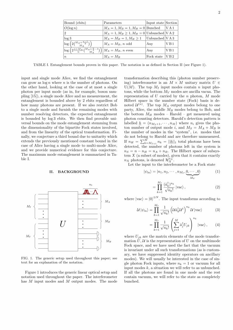
B. Optimal Bell state generation

MI

MV

MA = 2

MB = 2

MH

U

FIG. 3. The setup used in Section III B with four photonsin eight modes; MI = n = 4, MV = 4, MA = MB = 2,MH = 4. We give extensive numerical evidence for optimalBell state generation using this setup when looking for specificBell states as output.

The previous section showed that Bell state generationwith non-zero success probability requires at least fourphotons. Two schemes which accomplish this task usingfour photons use six [10] and eight [12, 13] modes, withsuccess probabilities of 2/27 and 1/4 respectively.

We performed a numerical search for a linear opticalBell state generator that gives a higher success probabil-ity. We used a gradient descent based optimization al-gorithm over M = 8 unitaries with n = 4 photon input.Numerical optimization was carried out in Python, usingthe BFGS algorithm from the SciPy library [20]. Thisalgorithm finds local minima so it needs to be run manytimes with different seed unitaries, which were randomlyselected according to the Haar measure.

The cost function we consider is based on the overlapwith the desired Bell states. We allow for six differentBell states, which in the Fock basis after measurementcorrespond to |B1,2〉 = (|1010〉 ± |0101〉)/

√2, |B3,4〉 =

(|1001〉 ± |0110〉)/√

2 and |B5,6〉 = (|1100〉 ± |0011〉)/√

2,where the latter can be corrected to the usual dual-railqubit encoding using a switch [13]. After detecting mea-surement pattern h, the overlap between each of these

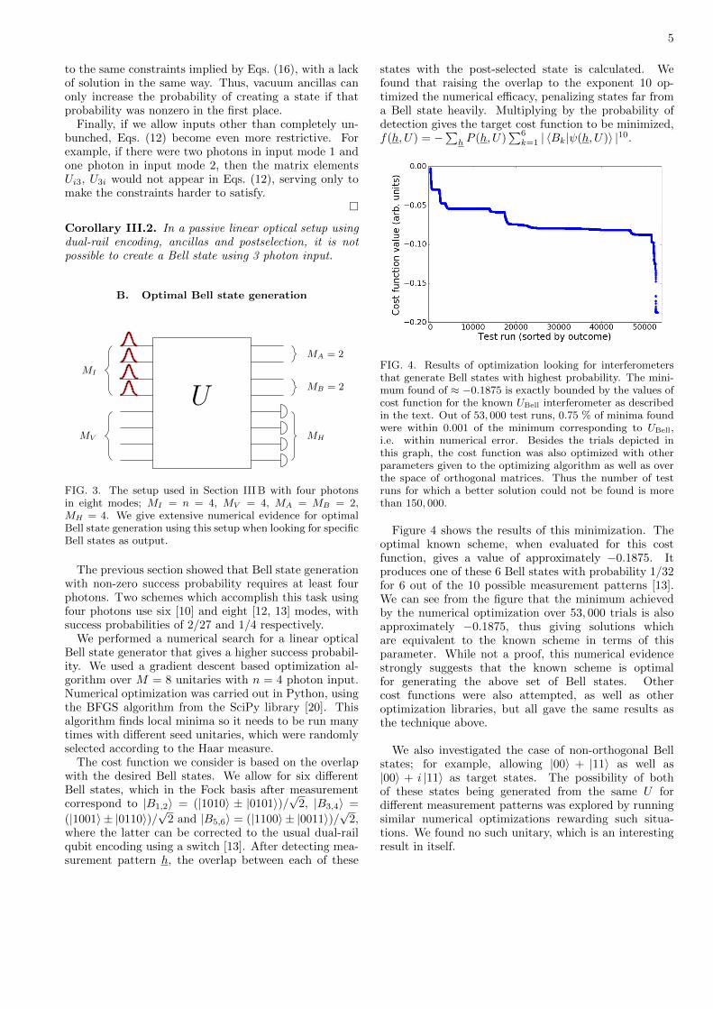
states with the post-selected state is calculated. Wefound that raising the overlap to the exponent 10 op-timized the numerical efficacy, penalizing states far froma Bell state heavily. Multiplying by the probability ofdetection gives the target cost function to be minimized,f(h, U) = −

∑h P (h, U)

∑6k=1 | 〈Bk|ψ(h, U)〉 |10.

FIG. 4. Results of optimization looking for interferometersthat generate Bell states with highest probability. The mini-mum found of ≈ −0.1875 is exactly bounded by the values ofcost function for the known UBell interferometer as describedin the text. Out of 53, 000 test runs, 0.75 % of minima foundwere within 0.001 of the minimum corresponding to UBell,i.e. within numerical error. Besides the trials depicted inthis graph, the cost function was also optimized with otherparameters given to the optimizing algorithm as well as overthe space of orthogonal matrices. Thus the number of testruns for which a better solution could not be found is morethan 150, 000.

Figure 4 shows the results of this minimization. Theoptimal known scheme, when evaluated for this costfunction, gives a value of approximately −0.1875. Itproduces one of these 6 Bell states with probability 1/32for 6 out of the 10 possible measurement patterns [13].We can see from the figure that the minimum achievedby the numerical optimization over 53, 000 trials is alsoapproximately −0.1875, thus giving solutions whichare equivalent to the known scheme in terms of thisparameter. While not a proof, this numerical evidencestrongly suggests that the known scheme is optimalfor generating the above set of Bell states. Othercost functions were also attempted, as well as otheroptimization libraries, but all gave the same results asthe technique above.

We also investigated the case of non-orthogonal Bellstates; for example, allowing |00〉 + |11〉 as well as|00〉 + i |11〉 as target states. The possibility of bothof these states being generated from the same U fordifferent measurement patterns was explored by runningsimilar numerical optimizations rewarding such situa-tions. We found no such unitary, which is an interestingresult in itself.

6

Though the complexity of the problem grows quickly,we also looked at how the situation changes with highernumbers of input photons and modes. We numericallyoptimized over n = 5, M = 10 using a similar algorithmand no improved solutions were found over 5000 runs.Similarly, we checked n = 6, M = 12 over 1000 runs andhere as well there was no improvement over the −0.1875result for n = 4, M = 8.

IV. RANDOM UNITARIES

In this section, we move from the dual-rail qubit en-coding of Section III to mode entanglement in Section V.First, we look at how much mode entanglement can begenerated with random elements of the unitary group,which we can then use to compare with the dual-rail en-coding. We do so by setting Alice and Bob’s numberof modes to 2, and numerically computing the averageamount of entanglement over measurement patterns. No-tice that this is different from the setting in Section III,where we aimed to get a maximally entangled Bell statewith the highest possible probability. Here and in therest of this work we will study this average entanglement,namely

〈S(U)〉H =∑h

P (h, U)S(ρA(h, U)). (18)

The expectation over the unitary group (for fixed M andn) is then 〈S〉H,U =

∫U(M)

dU 〈S(U)〉H , where dU is the

normalized Haar measure.

FIG. 5. The expectation, over the unitary group, of the aver-age, over measurement patterns, mode entanglement versusthe number of modes M , for various numbers of unbunchedinput photons. MA = MB = 2, and if the number of photonsn is smaller than M , vacuum input modes are added. Thenumber of heralding detectors is MH = M −MA −MB . Theentanglement for a single unitary U is averaged over all mea-surement patterns, and subsequently averaged over 100,000randomly Haar-sampled unitaries U . Colours and symbolsrepresent different number of input photons, with 2 ≤ n ≤ 7.

Figure 5 shows the numerical results. We notice thatoften the average is higher than 1 ebit, which is themaximum we can achieve in dual-rail qubit encoding.Adding input photons for the same M increases theaverage entanglement, while adding vacuum ancillasdecreases it. We see that the average entanglement ofn + 1 photons in M + 1 modes can be lower than thatfor M and n (see n = M = 5 and 6). That is, wedo not expect more average entanglement by adding aphoton at the cost of adding another mode. Further, wenote that even with 2 photons, there is more averageentanglement generated than in the optimal Bell stategenerator with 4 photons. We explore this in more detailfor a better comparison.

FIG. 6. Numerical evaluation of 〈S(U)〉H for 100, 000 uni-taries U chosen using the Haar measure in the case MA =MB = 2, MH = 4, and n = 4 unbunched input photons.Average entanglement for a given U was calculated accordingto Equation (18) and then binned in one of 100 bins with aminimum of 0 and maximum obtained in the samples. Thered dot marks the value of average entanglement that theBell generating unitary from Section III B can give, denotedas UBell, if all of its output states were used.

In the usual Bell state generation scenario discussed inSection III B, if the measurement outcome indicates thatthe output state is outside of the qubit subspace, theoutput is discarded. Here we include the entanglementof the discarded states in accordance with Eq. (18). Wecompare the optimal Bell state generator to random uni-taries with the same parameters; MA = MB = 2, n = 4and M = 8.

In Fig. 6 we see the results of the comparison. Firstly,in Section III B we saw that the probability of gettinga Bell state for a state correctable with a single switchis 3/16 [13]. A Bell state gives a single ebit, and if allthe other states are discarded, the average entanglementwould be 0.1875 ebits. If all the outputs from this unitarywere counted towards average entanglement as discussedin the previous paragraph (where Equation 18 is utilized),the entanglement obtained is marked on the Figure 6as UBell. As we can see from the graphs, UBell gives amarkedly lower amount of entanglement than what could

7

be generated on average with a random unitary on thesame number of modes.

V. MODE ENTANGLEMENT

The previous section shows that, on average, randomunitaries give significantly more mode entanglement thandual-rail encoding. We therefore turn our attention tothe investigation of mode rather than qubit entanglementas defined in Section II.

Equation (6) states that the total system Hilbertspace is a direct sum of Hilbert subspaces such thatthe sum of Alice and Bob’s photon numbers is nS , thenumber of photons left after heralding. Let ρAB =|ψS(h, U)〉 〈ψS(h, U)| as in Eq. (5). Alice’s reduced den-sity matrix is

ρA(h, U) = TrB [ρAB(h, U)] (19)

=∑b′′

〈b′′|

∑a,b,a′,b′

CabCa′b′ |ab〉 〈a′b′|

|b′′〉=∑a,a′

∑b

CabCa′b

|a〉 〈a′| , (20)

where only the terms with ‖a‖1 = ‖a′‖1 are non-zero,because ‖b‖1 = ‖b′‖1 = ‖b′′‖1 and nS = ‖a‖1 + ‖b‖1 =‖a′‖1 + ‖b′‖1. Therefore, there exists a Fock basis or-dering in which Alice’s reduced state is block diagonal,which allows us to derive a bound on the entanglement(see Section V B 1). In the case that Alice has a singlemode, this implies her state is diagonal in Fock basis.The total number of orthogonal states available to Aliceis

dim(HnS

A ) =

nS∑nA=0

(MA + nA − 1

nA

)=

(MA + nS

nS

).

(21)In Section V A, we find entanglement bounds when

Alice only has one mode. The bound depends on theinput state; if the input photons are bunched in a singlemode, entanglement is unbounded as the number of pho-tons increases. Surprisingly, if the input is unbunched,we find a constant bound independent of the number ofBob’s modes and independent of the number of photons.More general bounds can be found, though they are alsomore loose. In Section V B 1 we give the bound on en-tanglement due to the block diagonal structure of Alice’sreduced density matrix in Fock basis. In Section V B 2we give a bound which is a consequence of the linearity ofthe mode transformations. Unlike in Sec. V A, neither ofthese bounds depend on the unitarity of the mode trans-formations, which we expect should affect the amount ofentanglement that can be achieved. In Section V C weconjecture a general unitarity bound based on numericalevidence.

A. Entanglement when Alice has a single mode

1. Entanglement for bunched input can be unbounded

First, we show that mode entanglement is unboundedif we are not restricted to unbunched input.

MI = 1

MV = 1

MA = 1

MB = 1U...

n

FIG. 7. The setup used in Section V A 1, where we consideronly M = 2 modes. The input consists of all n photonsbunched in the top mode; MI = MV = MA = MB = 1, MH =0. We prove that in this setup maximal entanglement growsas logn. The special case where U is a balanced beamsplitterwas analyzed in [21].

Proposition V.1. Let the input into a M = 2 inter-ferometer consist of n photons bunched in a single mode(see Figure 7). Then the entanglement across the twooutput modes is at most O(log n) ebits, which is achievedwhen U is a balanced beamsplitter.

Proof. Parameterize the M = 2 unitary matrix U act-ing on Alice and Bob’s single mode Hilbert spaces as

U =

[c d

−d∗ c∗

], (22)

where |c|2 + |d|2 = 1. The output state is

|n0〉 =(a†1

)n/√n! |0〉

7→(ca†1 − d∗a

†2

)n/√n! |0〉

=1√n!

n∑k=0

(n

k

)(ca†1)k(−d∗a†2)n−k |0〉

=1√n!

n∑k=0

(n

k

)ck(−d∗)n−k

√k!√

(n− k)! |k〉 |n− k〉

=

n∑k=0

√(n

k

)ck(−d∗)n−k |k〉 |n− k〉 . (23)

When Alice has only one mode, her reduced density ma-trix is diagonal in the Fock basis, so we can find thespectrum of her state directly from the above equations:

λk =

(n

k

)(|c|2)k(|d|2)n−k =

(n

k

)(|c|2)k(1− |c|2)n−k.

(24)

This is a binomial distribution with a ‘success’ proba-bility of p = |c|2. The entropy of the binomial distribu-tion for a fixed p is 1/2 log2 (2πen · p · (1− p))+O(1/n)∗.

∗ From, e.g., the de Moivre-Laplace Theorem

8

Thus we see that the entanglement bound is O(log n),where n is the number of photons. The constant prefac-tor is maximized for p = |c|2 = |d|2 = 1/2, whence the en-tropy of Alice’s state is 1/2 log2 (2πen · 1/2 · (1− 1/2))+O(1/n) = 1/2 log2 (πen/2)+O(1/n). Finally, notice thatsolutions to Equation (22) where |c|2 = |d|2 = 1/2 are afamily of balanced beamsplitters. �This is in stark contrast to the situation where the inputis unbunched, where we will see in the next section thatthe entanglement is bounded by a constant.

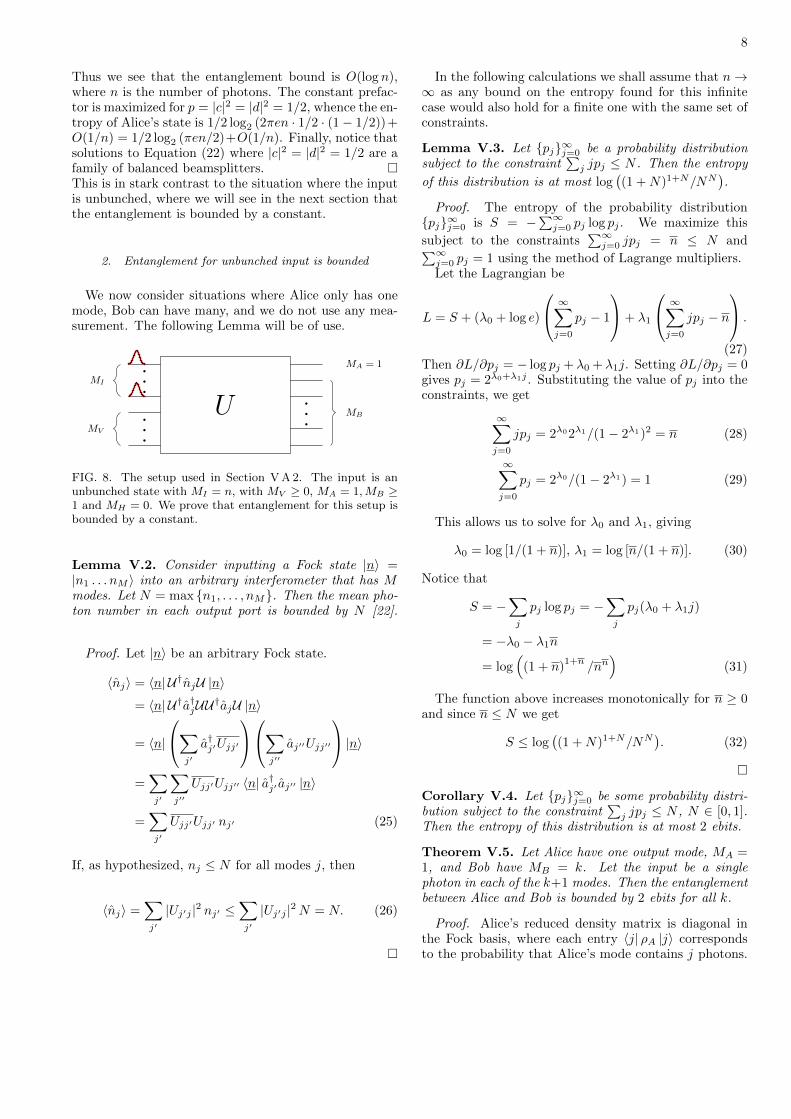
2. Entanglement for unbunched input is bounded

We now consider situations where Alice only has onemode, Bob can have many, and we do not use any mea-surement. The following Lemma will be of use.

......

...

MI

MV

MA = 1

MBU

FIG. 8. The setup used in Section V A 2. The input is anunbunched state with MI = n, with MV ≥ 0, MA = 1,MB ≥1 and MH = 0. We prove that entanglement for this setup isbounded by a constant.

Lemma V.2. Consider inputting a Fock state |n〉 =|n1 . . . nM 〉 into an arbitrary interferometer that has Mmodes. Let N = max {n1, . . . , nM}. Then the mean pho-ton number in each output port is bounded by N [22].

Proof. Let |n〉 be an arbitrary Fock state.

〈nj〉 = 〈n| U†njU |n〉

= 〈n| U†a†jUU†ajU |n〉

= 〈n|

∑j′

a†j′Ujj′

∑j′′

aj′′Ujj′′

|n〉=∑j′

∑j′′

Ujj′Ujj′′ 〈n| a†j′ aj′′ |n〉

=∑j′

Ujj′Ujj′ nj′ (25)

If, as hypothesized, nj ≤ N for all modes j, then

〈nj〉 =∑j′

|Uj′j |2 nj′ ≤∑j′

|Uj′j |2N = N. (26)

�

In the following calculations we shall assume that n→∞ as any bound on the entropy found for this infinitecase would also hold for a finite one with the same set ofconstraints.

Lemma V.3. Let {pj}∞j=0 be a probability distributionsubject to the constraint

∑j jpj ≤ N . Then the entropy

of this distribution is at most log((1 +N)1+N/NN

).

Proof. The entropy of the probability distribution{pj}∞j=0 is S = −

∑∞j=0 pj log pj . We maximize this

subject to the constraints∑∞j=0 jpj = n ≤ N and∑∞

j=0 pj = 1 using the method of Lagrange multipliers.Let the Lagrangian be

L = S + (λ0 + log e)

∞∑j=0

pj − 1

+ λ1

∞∑j=0

jpj − n

.

(27)Then ∂L/∂pj = − log pj + λ0 + λ1j. Setting ∂L/∂pj = 0gives pj = 2λ0+λ1j . Substituting the value of pj into theconstraints, we get

∞∑j=0

jpj = 2λ02λ1/(1− 2λ1)2 = n (28)

∞∑j=0

pj = 2λ0/(1− 2λ1) = 1 (29)

This allows us to solve for λ0 and λ1, giving

λ0 = log [1/(1 + n)], λ1 = log [n/(1 + n)]. (30)

Notice that

S = −∑j

pj log pj = −∑j

pj(λ0 + λ1j)

= −λ0 − λ1n

= log(

(1 + n)1+n

/nn)

(31)

The function above increases monotonically for n ≥ 0and since n ≤ N we get

S ≤ log((1 +N)1+N/NN

). (32)

�

Corollary V.4. Let {pj}∞j=0 be some probability distri-bution subject to the constraint

∑j jpj ≤ N , N ∈ [0, 1].

Then the entropy of this distribution is at most 2 ebits.

Theorem V.5. Let Alice have one output mode, MA =1, and Bob have MB = k. Let the input be a singlephoton in each of the k+1 modes. Then the entanglementbetween Alice and Bob is bounded by 2 ebits for all k.

Proof. Alice’s reduced density matrix is diagonal inthe Fock basis, where each entry 〈j| ρA |j〉 correspondsto the probability that Alice’s mode contains j photons.

9

By Lemma V.2, this distribution satisfies the conditionsof Corollary V.4. Thus the von Neumann entropy of thisstate is bounded by 2 for any k, as the bound which holdsfor k →∞ also holds for any finite k as well. �

Notice that extra vacuum modes will not increase thislimit on the entanglement as the limit is due to the ex-pected number of photons in Alice’s mode being at most1. We see that despite the fact that the dimension ofAlice’s Hilbert space grows with the number of photonsas n + 1, and Bob’s can be even larger, the maximumentanglement is severely constrained to be less than 2ebits.

Because we are interested in the average entanglement,the result will hold for heralding as well:

Corollary V.6. Let Alice have one output mode, MA =1, while Bob and Harold have MB + MH = k. Let theinput be a single photon in each of the k+1 modes. Thenthe entanglement between Alice and Bob is bounded by 2ebits for all k.

Proof. No LOCC operation can increase the amount ofentanglement in the system on average [23]. Therefore,〈S(U)〉H =

∑h P (h, U)S(ρA(h, U)) ≤ S(ρA(U)), where

ρA(U) is Alice’s reduced density matrix before any mea-surement, and by Theorem V.5, S(ρA(U)) ≤ 2 ebits. �

We can also examine inputs that have different num-bers of bunched photons. If the highest number of pho-tons in a single input mode is N , as per Lemma V.2,the expected number of photons in Alice’s mode willthen be bounded by N . Because the function whichbounds the entropy, Eq. (32), is monotonically increas-ing, the entropy of Alice’s (diagonal) state (p0, . . . , pn) isat most log

((1 +N)1+N/NN

)by Lemma V.3. In the ex-

treme case where all the photons are bunched in a singlemode, S scales as O(log(N + 1)), consistent with Propo-sition V.1.

3. Entanglement when Bob also has a single mode

In this section we consider a similar setup to the pre-vious section, except now we fix the number of Bob’smodes to 1 and assign the rest to Harold. Recall thatwe are interested in generating the highest amount of en-tanglement between Alice and Bob on average, thus theprobability of detection patterns must be taken into ac-count. More precisely, we are looking for the maximumof 〈S(U)〉H =

∑h P (h, U)S(ρA(h, U)). Some patterns

might yield a state with high entanglement, but be veryunlikely to occur. In a practical setting we might preferstates that are less entangled but we can generate moreconsistently.

We first prove a technical lemma that will be usefullater.

Lemma V.7. Given a probability distribution(p0, . . . , pn) such that

∑nj=0 jpj = 1, the sum

. ..

1

2

3

4

M − 1

M

MA = 1

MB = 1

MH

W

FIG. 9. The setup used in Section V A 3, where M = n,MA = MB = 1, and MH ≥ 1. An arbitrary M mode in-terferometer can be decomposed into M(M + 1)/2 two-modeinterferometers [24, 25]. Note that this also applies to an ar-bitrary M − 1 mode sub-interferometer (blue). By focusingon the only component that entangles Alice and Bob (red),we show that the maximum entanglement is the M = n = 2value of log 3 ebits.

∑nj=0 pj log (j + 2) is bounded by log 3 which can be

achieved by p1 = 1 and pk = 0 for k ∈ {0, 2, 3, . . . , n}.

Proof. Since f(x) = log (x+ 2) is a concave function,

by Jensen’s inequality∑nj=0 pjf(j) ≤ f

(∑nj=0 pjj

)=

f(1) = log 3, which is achieved by substituting p1 = 1and pk = 0 for k ∈ {0, 2, 3, . . . , n}. �

Theorem V.8. Consider an interferometer with M ≥ 3modes, where both Alice and Bob have one mode and theother output modes are measured using photon countingdetectors. Let the input be the n = M unbunched Fockstate. Then the maximal average entanglement that canbe created between Alice and Bob is log 3 ebits.

Proof. First, notice that the average entanglementachievable by an M = 2 interferometer can be achievedfor M ≥ 2 by having modes 3 to M transform trivially,since photons in these modes will be detected with unitprobability. Thus max 〈S(UM )〉H ≥ max 〈S(UM=2)〉H =log 3 ebits, ∀M ≥ 3. The interferometer given in SectionV D, Eq. (43) below achieves this.

Any U ∈ U(M) can be decomposed as in Fig. 9. Thenthe bottom left triangle (colored blue in the figure) is aunitary V ∈ U(M − 1). Since the input is unbunched,Lemma V.2 implies that each output from V has a meanphoton number of 1. In particular, Bob’s mode beforebeamsplitterW (red in the figure) will satisfy

∑k kqk = 1

where k is the number of photons occuring with proba-bility qk. Since the remaining beamsplitters (white in thefigure) act only on Bob and Harold’s systems, they haveno effect on Alice’s reduced state and can therefore beignored.

Let the probability of detecting pattern h be ph, andthe probability of detecting a total of nH = ‖h‖1 photons

10

be pnH=∑h:‖h‖1=nH

ph. The average entanglement is

〈S(U)〉H =∑h

phS(ρA(h))

=

n∑nH=0

pnH

∑h:‖h‖1=nH

ph/pnHS(ρA(h))

≤n∑

nH=0

pnH

∑h:‖h‖1=nH

ph/pnHlog (n− nH + 1)

=

n−1∑nH=0

pnHlog (n− nH + 1), (33)

where we’ve used the fact that the entanglement ofS(ρA(h)) is upper bounded by the Schmidt rank log(n−nH + 1).

As the photon number found in modes 1 and 2 isset before the beamsplitter W , if nH photons havebeen detected, then there were already nH photons inmodes 3 through M . Alice contributes one photonthrough her mode to their joint system, which impliesthat Bob must contribute n − nH − 1 photons throughmode 2, occurring with probability qn−nH−1. ThereforepnH

= qn−nH−1 and recall that Bob’s probability distri-

bution is constrained by∑n−1k=0 kqk = 1. By Lemma V.7∑n−1

nH=0 qn−nH−1 log (n− nH + 1) =∑n−1j=0 qj log (j + 2)

is maximized for j = n−nH−1 = 1, that is q1 = 1, yield-ing 〈S(U)〉H ≤ log 3. This also implies that nH = n − 2photons are detected in the optimal situation. �

Note that this agrees with the bound in Theo-rem V.5 found in the previous section, which followsfrom the entanglement measure property 〈S(U)〉H =∑h P (h, U)S(ρA(h, U)) ≤ S(ρA(U)), where ρA(U) is Al-

ice’s reduced density matrix before any measurement.Here the maximum entanglement is log 3 < 2 ebits.Moreover, adding more vacuum input modes will not af-fect this bound, as this would only change Bob’s expectednumber of photons before the beamsplitter W to be atmost 1 instead of exactly 1 as per Lemma V.2.

B. Entanglement when Alice has many modes

In this section we give two bounds on entanglementfor more general situations when Alice has more thanone mode, based on the Schmidt rank of Alice’s reducedstate. They are independent of the input state or any in-terferometer transformation, depending only on the givennumber of photons and modes; we assume the latter isthe same for both Alice and Bob. This generality comesat a price, however, in that the bounds loosen; we willdiscuss a conjectured tighter bound in the following sec-tion.

1. Dimensionality

By looking solely at the dimensions of Alice and Bob’sHilbert spaces, we can derive an entanglement bound asfollows.

Proposition V.9. Let Alice’s and Bob’s joint postse-lected state have a total of nS photons. Let Alice andBob have MA = MB modes. The Schmidt rank, ω, is atmost

ω = 2

(MA + nS−1

2nS−1

2

)nS odd, (34)

ω = 2nS +MA

nS

(MA + nS

2 − 1nS

2 − 1

)nS even. (35)

Proof. Let Alice’s and Bob’s joint state be|ψS(h, U)〉 =

∑k,j Ckj(h, U) |k〉A ⊗ |j〉B , where we in-

clude the possibility of no measurement (MH = 0). TheSchmidt decomposition is achieved by a state dependentchange of basis such that

|ψS(h, U)〉 =

min(dimHA,dimHB)∑q=1

λq |q〉A ⊗ |q〉B , (36)

where {|q〉A,B} are orthonormal bases for A and B, re-spectively.

Writing this state in terms of Alice andBob’s photon numbers we have |ψS(h, U)〉 =∑nS

nA=0 |ψnA,nB

S (h, U)〉 with nB = nS − nA. The

overlap 〈ψnA,nB

S (h, U)|ψn′A,n′B

S (h, U)〉 = 0 for nA 6= n′A,nB 6= n′B as these states belong to different Hilbertsubspaces in the direct sum. The reduced density matrixis block diagonal – each block corresponds to a different(nA, nB) combination. We may therefore consider eachsubspace individually, where the maximal Schmidtrank is min(dimHnA

A ,dimHnB

B ). The total number ofSchmidt coefficients is therefore at most

ω =

nS∑nA=0

min{dimHnA

A ,dimHnB

B } (37)

=

nS∑nA=0

min

{(MA + nA − 1

nA

),

(MB + nB − 1

nB

)}.

(38)

For MA = MB this gives the result. �Since the entanglement is given by the number of

nonzero Schmidt coefficients, this gives a bound on theentanglement S ≤ log(ω).

2. Linearity bound

Here we consider a bound due to the linearity of theinterferometer transformations. In the following we donot assume anything about the form of the input Fockstate, nor whether measurement occurs or not.

11

Proposition V.10. Given an n photon Fock state asinput to a M -mode linear optical device, with Alice andBob having MA and MB output modes respectively, themaximal entanglement achievable between Alice and therest of the modes for any state is bounded by n ebits.

Proof. Starting with the arbitrary linear optical modetransformation in Eq.(4), we can group the sum into Al-ice’s modes and the ‘rest’:

a†k 7→M∑j=1

a†jUjk =

MA∑j=1

a†jUjk +

M∑j=MA+1

a†jUjk

=: Ak(U) + Rk(U). (39)

The degree one polynomials Ak(U), Rk(U) in the cre-ation operators are not canonical raising operators, be-cause e.g. [Ak(U), Ak′(U)] 6= δkk′ . This means that dif-

ferent monomials in {Ak(U)}k do not necessarily give riseto orthogonal states; however, this can only reduce theSchmidt rank of the resulting state.

An arbitrary input Fock state is of the form∏Mk=1(a†k)nk/

√nk! |vac〉, so that the output state is of

the form

M∏k=1

1√nk!

(Ak(U) + Rk(U))nk |vac〉 (40)

i.e. it is a product of n terms, not all of which are neces-sarily different. We can rewrite it as

Nn∏k=1

(Ajk(U) + Rjk(U)) |vac〉 , (41)

where jk ∈ {1, . . . ,M} and N is the necessary normal-ization. The highest number of monomial terms in thisproduct is bounded by 2n and after tracing out Bob andHarold this also bounds the number of monomial termsthat can be in Alice’s reduced state. �

Consider a balanced 50:50 beam splitter coupling oneof Alice’s modes (say k) to one of Bob’s modes (sayk + MA). If Alice’s mode contained one input photonand Bob’s none, we get 1 ebit of entanglement. Propo-sition V.10 tells us we can only get up to n ebits usingn photons, so as long as n ≤ MA = MB , a beamsplittercoupling mode k with mode k+MA for k = 1 through nin this way would give us a state that achieves the bound.

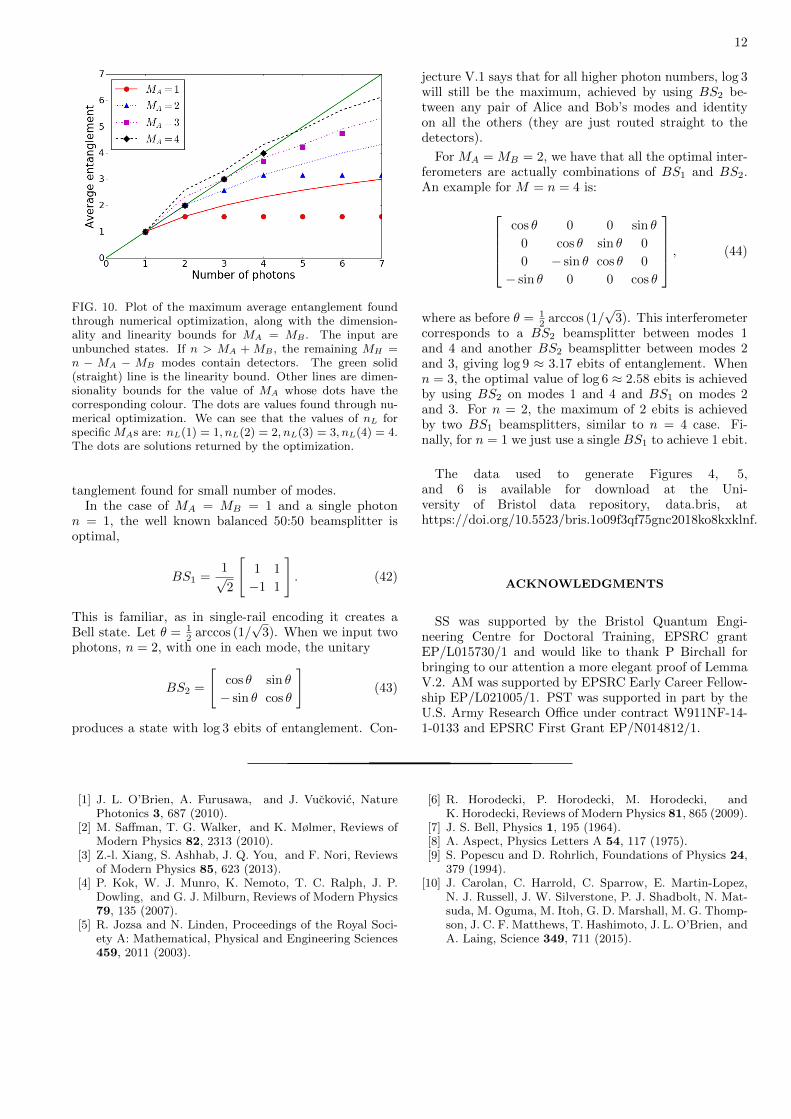
The dimensionality (Section V B 1) and linearitybounds above hold for all M and all n. We can findnumerically the photon number nL(MA) ∈ N, which de-pends on the number of Alice’s modes. For a given MA

it represents the number of photons up to which the lin-earity bound is smaller than the dimensionality bound.For n > nL(M), the dimensionality bound is a tighterlimit on the entanglement (see Figure 10).

C. Hints of another bound

In this section we explore a potential bound that ismotivated by numerical evidence (see Figure 10). Whileadding more photons to the interferometer increases thesize of Alice’s and Bob’s Hilbert spaces, and accordingto the results from the previous section should allow forhigher amounts of entanglement, we see that this is notwhat happens in general (assuming the number of modesthat Alice and Bob have are fixed). Based on the analyt-ical results from Section V A and the numerical evidencefor all cases up to n = 7 photons and MA = MB = 3modes, we make a conjecture that there is another boundwhich seems to arise from the unitarity of the mode trans-formation.

Conjecture V.1. For n unbunched photons input intoan interferometer with MA Alice and MB Bob outputmodes with n > MA + MB , the average amount ofentanglement, obtained over Harold’s measurements, isbounded above by the maximal average amount of en-tanglement achieved when n = MA +MB .

We provide numerical evidence supporting this “uni-tarity bound” for various numbers of input photons andmodes. We assume that the input states are unbunched,ancillas and measurement are allowed, and Alice and Bobhave the same number of modes; MI = n, MV ≥ 0,MA = MB ≥ 1 and MH ≥ 0.

Propositions V.9 and V.10 provide tight entanglementbounds when all input photons are kept in the system,i.e. when there is no detection. We know that it is pos-sible to postselect states that exceed these bounds, butbecause we are interested in average entanglement thesecases must be weighted with their heralding probabilities.Our findings are consistent with a generic trade off be-tween these two quantities, leading to a bounded averageentanglement.

Figure 10 shows the results of numerical optimizationof the average entanglement given by Eq. (18) for vari-ous numbers of input photons and modes. We can seehow the linearity and dimensionality bounds of Sec. V Bare indeed limiting the entanglement. We also see theappearance of what looks like a third bound, seeminglywhen the number of photons is larger than the total num-ber of modes in the system (MA + MB). This new be-haviour is not captured by the bounds we have obtainedand we conjecture that it is due to the unitarity of the in-terferometric transformation. This leads to the hypoth-esis that the maximum possible average entanglement,in situations with unbunched input and Alice and Bobhave the same number of modes, can be reached using a(MA+MB)-mode interferometer with MA+MB photons.

D. Optimal interferometers

Finally, in this section we report some of the explicitinterferometers (unitaries) that produce the optimal en-

12

FIG. 10. Plot of the maximum average entanglement foundthrough numerical optimization, along with the dimension-ality and linearity bounds for MA = MB . The input areunbunched states. If n > MA + MB , the remaining MH =n − MA − MB modes contain detectors. The green solid(straight) line is the linearity bound. Other lines are dimen-sionality bounds for the value of MA whose dots have thecorresponding colour. The dots are values found through nu-merical optimization. We can see that the values of nL forspecific MAs are: nL(1) = 1, nL(2) = 2, nL(3) = 3, nL(4) = 4.The dots are solutions returned by the optimization.

tanglement found for small number of modes.In the case of MA = MB = 1 and a single photon

n = 1, the well known balanced 50:50 beamsplitter isoptimal,

BS1 =1√2

[1 1

−1 1

]. (42)

This is familiar, as in single-rail encoding it creates aBell state. Let θ = 1

2 arccos (1/√

3). When we input twophotons, n = 2, with one in each mode, the unitary

BS2 =

[cos θ sin θ

− sin θ cos θ

](43)

produces a state with log 3 ebits of entanglement. Con-

jecture V.1 says that for all higher photon numbers, log 3will still be the maximum, achieved by using BS2 be-tween any pair of Alice and Bob’s modes and identityon all the others (they are just routed straight to thedetectors).

For MA = MB = 2, we have that all the optimal inter-ferometers are actually combinations of BS1 and BS2.An example for M = n = 4 is:

cos θ 0 0 sin θ

0 cos θ sin θ 0

0 − sin θ cos θ 0

− sin θ 0 0 cos θ

, (44)

where as before θ = 12 arccos (1/

√3). This interferometer

corresponds to a BS2 beamsplitter between modes 1and 4 and another BS2 beamsplitter between modes 2and 3, giving log 9 ≈ 3.17 ebits of entanglement. Whenn = 3, the optimal value of log 6 ≈ 2.58 ebits is achievedby using BS2 on modes 1 and 4 and BS1 on modes 2and 3. For n = 2, the maximum of 2 ebits is achievedby two BS1 beamsplitters, similar to n = 4 case. Fi-nally, for n = 1 we just use a single BS1 to achieve 1 ebit.

The data used to generate Figures 4, 5,and 6 is available for download at the Uni-versity of Bristol data repository, data.bris, athttps://doi.org/10.5523/bris.1o09f3qf75gnc2018ko8kxklnf.

ACKNOWLEDGMENTS

SS was supported by the Bristol Quantum Engi-neering Centre for Doctoral Training, EPSRC grantEP/L015730/1 and would like to thank P Birchall forbringing to our attention a more elegant proof of LemmaV.2. AM was supported by EPSRC Early Career Fellow-ship EP/L021005/1. PST was supported in part by theU.S. Army Research Office under contract W911NF-14-1-0133 and EPSRC First Grant EP/N014812/1.

[1] J. L. O’Brien, A. Furusawa, and J. Vuckovic, NaturePhotonics 3, 687 (2010).

[2] M. Saffman, T. G. Walker, and K. Mølmer, Reviews ofModern Physics 82, 2313 (2010).

[3] Z.-l. Xiang, S. Ashhab, J. Q. You, and F. Nori, Reviewsof Modern Physics 85, 623 (2013).

[4] P. Kok, W. J. Munro, K. Nemoto, T. C. Ralph, J. P.Dowling, and G. J. Milburn, Reviews of Modern Physics79, 135 (2007).

[5] R. Jozsa and N. Linden, Proceedings of the Royal Soci-ety A: Mathematical, Physical and Engineering Sciences459, 2011 (2003).

[6] R. Horodecki, P. Horodecki, M. Horodecki, andK. Horodecki, Reviews of Modern Physics 81, 865 (2009).

[7] J. S. Bell, Physics 1, 195 (1964).[8] A. Aspect, Physics Letters A 54, 117 (1975).[9] S. Popescu and D. Rohrlich, Foundations of Physics 24,

379 (1994).[10] J. Carolan, C. Harrold, C. Sparrow, E. Martin-Lopez,

N. J. Russell, J. W. Silverstone, P. J. Shadbolt, N. Mat-suda, M. Oguma, M. Itoh, G. D. Marshall, M. G. Thomp-son, J. C. F. Matthews, T. Hashimoto, J. L. O’Brien, andA. Laing, Science 349, 711 (2015).

13

[11] M. Gimeno-Segovia, P. Shadbolt, D. E. Browne, andT. Rudolph, Physical Review Letters 115, 020502 (2015).

[12] J. Joo, P. L. Knight, J. L. O’Brien, and T. Rudolph,Physical Review A 76, 052326 (2007).

[13] Q. Zhang, X.-H. Bao, C.-Y. Lu, X.-Q. Zhou, T. Yang,T. Rudolph, and J.-W. Pan, Physical Review A 77,062316 (2008).

[14] T. Rudolph, (2016), arXiv:1610.07128.[15] S. Aaronson and A. Arkhipov, Theory of Computing 9,

143 (2013).[16] F. Benatti, R. Floreanini, and U. Marzolino, Annals of

Physics 327, 1304 (2012).[17] F. Benatti, R. Floreanini, and U. Marzolino, Physical

Review A 85, 042329 (2012).[18] S. Scheel, (2004), arXiv:quant-ph/0406127.[19] K. Kieling, Linear optics quantum computing–

construction of small networks and asymptotic scaling,Ph.D. thesis, Imperial College London (2008).

[20] E. Jones, T. Oliphant, P. Peterson, et al., “SciPy: Opensource scientific tools for Python,” (2001–2017).

[21] W. Vogel and J. Sperling, Physical Review A 89, 052302(2014).

[22] J. P. Olson, K. R. Motes, P. M. Birchall, N. M. Studer,M. LaBorde, T. Moulder, P. P. Rohde, and J. P. Dowling,(2016), arXiv:1610.07128.

[23] M. Horodecki, Quantum Information & Computation 1,3 (2001).

[24] A. Hurwitz, Nachrichten von der Gesellschaft der Wis-senschaften zu Gottingen, Mathematisch-PhysikalischeKlasse 1897, 71 (1897).

[25] M. Reck, A. Zeilinger, H. J. Bernstein, and P. Bertani,Physical Review Letters 73, 58 (1994).