Generalized Tumor Dose for TreatmentPlanning Decision Support

by

Areli A. Zúñiga

A dissertation submitted in partial fulfillment ofthe requirements for the degree of

Doctor of Philosophy,(Medical Physics)

at the

University of Wisconsin–Madison

2015

Date of final oral examination: December 22nd, 2014.

The dissertation is approved by the following members of the Final Oral Committee:

Advisor Bhudatt Paliwal, Professor, Medical Physics and Human OncologyLarry DeWerd, Professor, Medical PhysicsMark Ritter, Professor, Medical Physics and Human OncologyRichard Chappell, Professor, Biostatistics & Medical Informatics and StatisticsBryan Bednarz, Assistant Professor, Medical Physics

© Copyright by Areli Zúñiga 2014

All Rights Reserved

i

To my partner and children.

ii

Contents

Acknowledgments vi

Abstract ix

Nomenclature x

List of Figures xi

List of Tables xv

1 Introduction 1

2 Background 52.1 Local Control (LC) . . . . . . . . . . . . . . . . . . . . . . . . . . . . . . . . 62.2 Tumor volume and LC . . . . . . . . . . . . . . . . . . . . . . . . . . . . . . 112.3 Linear quadratic model . . . . . . . . . . . . . . . . . . . . . . . . . . . . . . 112.4 Equivalent Uniform Dose (EUD) . . . . . . . . . . . . . . . . . . . . . . . . 132.5 Setup errors . . . . . . . . . . . . . . . . . . . . . . . . . . . . . . . . . . . . 162.6 Biologically based treatment planning . . . . . . . . . . . . . . . . . . . . . . 19

3 Local Control correlation 213.1 Introduction . . . . . . . . . . . . . . . . . . . . . . . . . . . . . . . . . . . . 213.2 Materials and methods . . . . . . . . . . . . . . . . . . . . . . . . . . . . . . 22

3.2.1 Patient cohorts . . . . . . . . . . . . . . . . . . . . . . . . . . . . . . 223.2.2 Analysis . . . . . . . . . . . . . . . . . . . . . . . . . . . . . . . . . . 24

3.3 Univariate local control prediction results . . . . . . . . . . . . . . . . . . . . 273.3.1 Vx and Dx parameters . . . . . . . . . . . . . . . . . . . . . . . . . . 273.3.2 All other parameters . . . . . . . . . . . . . . . . . . . . . . . . . . . 29

iii

3.3.3 Multivariate analysis . . . . . . . . . . . . . . . . . . . . . . . . . . . 323.3.4 EUDs . . . . . . . . . . . . . . . . . . . . . . . . . . . . . . . . . . . 33

3.4 Discussion . . . . . . . . . . . . . . . . . . . . . . . . . . . . . . . . . . . . . 39

4 cEUD modifications and generalized tumor dose (gTD) formulation 414.1 Introduction . . . . . . . . . . . . . . . . . . . . . . . . . . . . . . . . . . . . 414.2 Modified SF2 . . . . . . . . . . . . . . . . . . . . . . . . . . . . . . . . . . . 424.3 Generalized Tumor Dose (gTD) formulation . . . . . . . . . . . . . . . . . . 45

4.3.1 Derivation . . . . . . . . . . . . . . . . . . . . . . . . . . . . . . . . . 464.3.2 Parameter fitting methods . . . . . . . . . . . . . . . . . . . . . . . . 484.3.3 Results of gTD fitted to clinical outcome data . . . . . . . . . . . . . 50

4.4 Discussion . . . . . . . . . . . . . . . . . . . . . . . . . . . . . . . . . . . . . 55

5 Margin influence on LC 575.1 Introduction . . . . . . . . . . . . . . . . . . . . . . . . . . . . . . . . . . . . 575.2 Materials and methods . . . . . . . . . . . . . . . . . . . . . . . . . . . . . . 58

5.2.1 Motion simulation . . . . . . . . . . . . . . . . . . . . . . . . . . . . 585.2.2 Treatment planning and outcome data . . . . . . . . . . . . . . . . . 595.2.3 Model application . . . . . . . . . . . . . . . . . . . . . . . . . . . . . 615.2.4 Data analysis . . . . . . . . . . . . . . . . . . . . . . . . . . . . . . . 63

5.3 Results . . . . . . . . . . . . . . . . . . . . . . . . . . . . . . . . . . . . . . . 645.4 Discussion . . . . . . . . . . . . . . . . . . . . . . . . . . . . . . . . . . . . . 68

6 External gTD model validation 716.1 Introduction . . . . . . . . . . . . . . . . . . . . . . . . . . . . . . . . . . . . 716.2 Methods and material . . . . . . . . . . . . . . . . . . . . . . . . . . . . . . 72

6.2.1 Training cohort . . . . . . . . . . . . . . . . . . . . . . . . . . . . . . 726.2.2 Validation cohort . . . . . . . . . . . . . . . . . . . . . . . . . . . . . 736.2.3 Proposed predictive model . . . . . . . . . . . . . . . . . . . . . . . . 746.2.4 Performance measures . . . . . . . . . . . . . . . . . . . . . . . . . . 75

6.3 Results . . . . . . . . . . . . . . . . . . . . . . . . . . . . . . . . . . . . . . . 786.4 Discussion . . . . . . . . . . . . . . . . . . . . . . . . . . . . . . . . . . . . . 88

7 Conclusions and future directions 917.1 Conclusions . . . . . . . . . . . . . . . . . . . . . . . . . . . . . . . . . . . . 917.2 Future directions . . . . . . . . . . . . . . . . . . . . . . . . . . . . . . . . . 93

iv

Appendix A Implementation of gTD function in MatLab® 95

v

Acknowledgments

It would never have been possible to name each and everyone who played some part on this

adventure, but there are a few I could not help but mention.

First and foremost, I am forever grateful to Bhudatt Paliwal for his wisdom, sup-

port, encouragement, generosity and for always having the right words and giving selfless

advice, for accepting me as his student. Second, I thank Fulbright-CONICYT Chile, for

sponsoring me throughout my entire stay in the US giving me peace of mind to fully dedi-

cate myself to this project. I also would like to thank Joe Deasy for allowing me to participate

and receive support from his group, and for his feedback and suggestions for this research.

Thanks to all my defense committee members, Dr. Larry DeWerd, Dr. Mark Ritter, Dr.

Bryan Bednarz, Dr. Wolfgang Tomé and Dr. Richard Chappell. Mariela Porras, for every-

thing, from receiving me at your place at my arrival during an awful snow storm, to the

final encouraging words. Paulina Galavis and her family, for welcoming me at their home.

Regina Fulkerson, for caring for me all the time we were roommates. Keisha McCall, for

proofreading my thesis proposal and helping me through that process. I also would like

to thank the physicists and sta� in the Department of Medical Physics and Human Oncol-

ogy, JoAnn, Deb, Beth, Yacouba, Michell Anderle and Dianne, for making my life easier

paperwork-wise. I also need to thank the physicians who played an important role in this

project: Wade Thorstad, Je� Bradley and Cli� Robinson from WashU, and Nancy Lee and

vi

Andreas Rimmer from MSKCC. My friends, the ones I made here and the ones that sup-

ported and encourage me from home. Specially to Eugenio, who has always been there for

me with love and respect. Thank you all.

vii

Abstract

Modern radiation therapy techniques allow for improved target conformity and normal tissue

sparing. These highly conformal treatment plans have allowed dose escalation techniques

increasing the probability of tumor control. At the same time this conformation has in-

troduced inhomogeneous dose distributions, making delivered dose characterizations more

di�cult. The concept of equivalent uniform dose (EUD) characterizes a heterogeneous dose

distribution within irradiated structures as a single value and has been used in biologically

based treatment planning (BBTP); however, there are no substantial validation studies on

clinical outcome data supporting EUD’s use and therefore has not been widely adopted as

decision-making support.

These highly conformal treatment plans have also introduced the need for safety

margins around the target volume. These margins are designed to minimize geometrical

misses, and to compensate for dosimetric and treatment delivery uncertainties. The margin’s

purpose is to reduce the chance of tumor recurrence.

This dissertation introduces a new EUD formulation designed especially for tumor

volumes, called generalized Tumor Dose (gTD). It also investigates, as a second objective,

margins extensions for potential improvements in local control while maintaining or mini-

mizing toxicity.

viii

The suitability of gTD to rank LC was assessed by means of retrospective studies

in a head and neck (HN) squamous cell carcinoma (SCC) and non-small cell lung cancer

(NSCLC) cohorts. The formulation was optimized based on two datasets (one of each type)

and then, model validation was assessed on independent cohorts.

The second objective of this dissertation was investigated by ranking the probability

of LC of the primary disease adding di�erent margin sizes. In order to do so, an already

published EUD formula was used retrospectively in a HN and a NSCLC datasets.

Finally, recommendations for the viability to implement this new formulation into

a routine treatment planning process as well as the revision of safety margins to improve

local tumor control maximizing normal tissue sparing in SCC of the HN and NSCLC are

discussed.

ix

List of Figures

2.1 Head and neck cancer regions: paranasal sinuses, nasal cavity, oral cavity,

tongue, salivary glands, larynx, and pharynx (including the nasopharynx,

oropharynx, and hypopharynx). Picture taken from www.cancer.gov. . . . . 7

2.2 Essentially normal chest x-ray at first sight, there might be an early stage

lung cancer that cannot be seen using this image modality. Figure taken from

http://eishazinnerworld.blogspot.com. . . . . . . . . . . . . . . . . . . . . . 9

2.3 A survival curve using the standard LQ formula exp(≠–D ≠ —D2) where – =

0.2 and –/— = 3. The components of cell killing are equal where the curves

exp(≠–D) and exp(≠—D2) intersect. This occurs at dose D = –/— (3 Gy in

this example). Figure taken from http://ozradonc.wikidot.com. . . . . . . . 12

2.4 Example of immobilization device for head and neck and lung cancer treat-

ment. . . . . . . . . . . . . . . . . . . . . . . . . . . . . . . . . . . . . . . . 17

2.5 Scheme of ICRU definitions of di�erent treatment target volumes (Gross, Clin-

ical Internal and Planning Target Volumes), including internal margin (IM)

and setup margin (SM). Figure taken from ICRU 62. . . . . . . . . . . . . . 18

3.1 An example of non small cell lung treatment dose distributions of this cohort. 23

3.2 An example of head and neck dose distributions of this cohort. . . . . . . . 24

x

3.3 The receiver operating characteristic (ROC) curve. The dotted line shown in

the ROC curve represents a useless test that has no discriminatory power. . 26

3.4 Correlation results for V5 to V80 and D5 to D100 parameters of the Head and

Neck. Dotted line indicates statistically significant threshold (0.05). . . . . . 28

3.5 Correlation results for V5 to V80 and D5 to D100 parameters in NSCLC. Dotted

line indicates statistically significant threshold (0.05). . . . . . . . . . . . . . 30

3.6 Dependency of the EUDs on their respective parameters. . . . . . . . . . . . 35

3.7 cEUD dependency on di�erent Vref values. . . . . . . . . . . . . . . . . . . . 36

3.8 Dose response curves built using a logistic regression of the cEUD for HN and

NSCLC. . . . . . . . . . . . . . . . . . . . . . . . . . . . . . . . . . . . . . . 36

3.9 Response curves built using a logistic regression of the tumor volume for HN

and NSCLC. . . . . . . . . . . . . . . . . . . . . . . . . . . . . . . . . . . . . 37

3.10 Proliferation e�ect for NSCLC dataset. Tk=21 days, and Tp=3 days. . . . . . 38

3.11 Actuarial estimates for HN and NSCLC based on cEUD cuto�s. . . . . . . . 39

4.1 Maps of the AUC values for di�erent SF2 and k values for both datasets.

Dashed lines intersection represents a high correlation while keeping a radio-

biologically meaningful SF2 value. . . . . . . . . . . . . . . . . . . . . . . . . 44

4.2 Dose response curves built using a logistic regression of the cEUD with the

e�ective SF2 for HN and NSCLC. . . . . . . . . . . . . . . . . . . . . . . . . 45

4.3 Generalized tumor dose (gTD) dependency on its two variables (– and a) for

head and neck and NSCLC. . . . . . . . . . . . . . . . . . . . . . . . . . . . 50

4.4 Fitting distribution of parameter "a" for the NSCLC cohort after 200 bootstrap

samples. . . . . . . . . . . . . . . . . . . . . . . . . . . . . . . . . . . . . . . 52

4.5 Overlap and mean results of the validation distribution of parameter "a" for

both cohorts after 200 bootstrap samples. . . . . . . . . . . . . . . . . . . . 53

xi

4.6 Dose response curves built using a logistic regression of the newly proposed

gTD formulation, for HN and NSCLC. . . . . . . . . . . . . . . . . . . . . . 54

5.1 Example of dose volume histograms for GTV plus margins after motion sim-

ulation using 10 trials in NSCLC. From right to left, we have GTV, GTV

+2 mm, GTV +5 mm, GTV +10 mm, GTV +15 mm and GTV +20 mm,

respectively. The dashed lines represent the mean DD after motion simulation

and the colored area denotes the 3 sigma variation. . . . . . . . . . . . . . . 60

5.2 Description of the structures created for analysis of margin influence on local

control. . . . . . . . . . . . . . . . . . . . . . . . . . . . . . . . . . . . . . . 62

5.3 Results for the analysis of the margin influence on LC in HN. . . . . . . . . 65

5.4 Results for the analysis of the margin influence on LC in NSCLC . . . . . . 66

6.1 Normal probability plot of the Pearson chi squared test residuals for the gTD

model prediction applied to an independent HN cohort. . . . . . . . . . . . . 79

6.2 Normal probability plot of the Pearson chi squared test residuals for the gTD

model prediction applied to an independent NSCLC cohort. . . . . . . . . . 80

6.3 Model calibration curve for prediction of LC in a 113 HN patients from

MSKCC. The blue squares are the observed rates when patients are grouped

into 11 bins (the last bin containing 13 patients, and all other with 11 each),

with their respective error bars. The red line represents the linear trend of

the data, described by the equation also in red. . . . . . . . . . . . . . . . . 81

6.4 Model calibration curve for prediction of LC in a 116 NSCLC patients from

WU. The blue squares are the observed rates when patients are grouped into

11 bins (the last bin containing 16 patients, and all other with 11 each), with

their respective error bars. The red line represents the linear trend of the

data, described by the equation also in red. . . . . . . . . . . . . . . . . . . 82

xii

6.5 ROC plot for HN model validation. In this case AUC = 0.807, where AUC =

1 represents the perfect model. . . . . . . . . . . . . . . . . . . . . . . . . . . 83

6.6 the central mark is the median, the edges of the box are the 25th and 75th per-

centiles, the whiskers extend to the most extreme data points not considered

outliers, and outliers are plotted individually. . . . . . . . . . . . . . . . . . . 84

6.7 ROC plot for NSCLC model validation. AUC = 0.5 means that the model

does not perform better than random guess, and an AUC of 1 reflects the

perfect model.In this case AUC = 0.535 . . . . . . . . . . . . . . . . . . . . 85

6.8 Dose response curve computed from the proposed predictive model applied to

an external HN validation set. . . . . . . . . . . . . . . . . . . . . . . . . . . 86

6.9 Dose response curve computed from the proposed predictive model applied to

an external NSCLC validation set. . . . . . . . . . . . . . . . . . . . . . . . . 87

xiii

List of Tables

3.1 Statistically significant parameters and their correlation rank coe�cients on

univariate analysis for head and neck cohort. . . . . . . . . . . . . . . . . . . 31

3.2 Statistically significant parameters and their correlation rank coe�cients on

univariate analysis for NSCLC cohort. . . . . . . . . . . . . . . . . . . . . . 31

3.3 Comparison of statistically significant parameters on univariate analysis for

both datasets. . . . . . . . . . . . . . . . . . . . . . . . . . . . . . . . . . . . 32

3.4 Summary of Statistically significant model parameters results on univariate

analysis after performing cross-validation. . . . . . . . . . . . . . . . . . . . . 33

6.1 Logistic regression parameters for HN and NSCLC LC gTD models, obtained

in Section 4.3.3. . . . . . . . . . . . . . . . . . . . . . . . . . . . . . . . . . . 75

1

Chapter 1

Introduction

Local tumor control (LC) is associated with an increased survival rate of cancer patients.1

Di�erent treatment modalities, such as surgery, chemotherapy and radiotherapy, and sched-

ules are evaluated to provide patients with the best treatment choice possible. The goal is to

maximize LC while minimizing side e�ects. In radiotherapy (RT), highly conformal treat-

ment plans and techniques, such as intensity-modulated RT (IMRT), are currently the most

sophisticated ways to accomplish these aims. Furthermore, safety margins around the target

volume are used in order to account for positional uncertainties, minimizing the chances of

target miss. However, there is no universally accepted, nor validated, model used in clinical

practice to aid evaluate the probability of LC among possible treatment plans.

Several parameters that may influence the likelihood of local control, such as

patient-specific factors, tumor characteristics, dosimetric and treatment-related risk factors,

have been studied both as single predictors, and in multivariate analyses without definitive

results.2,3 The generalized equivalent uniform dose (gEUD), because of its simplicity and

easy implementation, has been adopted for some treatment planning systems (TPS) for op-

2

timization purposes. However, gEUD does not play a role in decision-making due to the lack

of independent validation studies.

A predictive model suitable for clinical use should reasonably classify LC and re-

currence among di�erent tumor types. It would have to be simple to implement, and able

to rank treatment plans, assisting the physician as a decision support tool.

This dissertation proposes the use of a new generalized tumor dose (gTD) formula

to predict LC probability for daily clinical use in treatment planning. This dissertation also

investigates the optimal margins around the gross-target volume to assure better LC and

less morbidity by means of outcome analysis.

The focus of Chapter 2 is on the ground concepts. It helps understand the impor-

tance of local control and the basis for the equivalent uniform dose modeling. It will also

review the linear quadratic model and give the foundation of setup errors needed to study

margins analysis. At the end of the chapter, an introduction to biologically based treatment

planning (BBTP) will be given.

In Chapter 3, local control correlation with LC is assessed in order to compare their

predictive performance to the newly proposed gTD formulation. Univariate and multivariate

analysis of all clinical and dosimetric parameters available, including the generalized and the

cell-kill equivalent uniform doses, were studied.

Chapter 4 describes first, a modification to the cEUD model that changes the

surviving fraction at 2 Gy linearly with tumor volume seeking for consistency with already

published radiobiological parameters. Second, it outlines the proposed gTD formulation

derivation along with parameter fitting results.

3

The impact of margin sizes in two di�erent datasets is described in Chapter 5. It

was done by analyzing how much di�erent margin sizes add to correlation with LC, after

computing a motion-simulated delivered dose distribution.

In Chapter 6 validation of the proposed gTD model will be examined to determine

its applicability. Model calibration and discrimination ability are investigated.

The final Chapter 7 summarizes all important findings of this dissertation and the

future work.

4

Chapter 2

Background

The primary goal of radiation therapy is to deliver a precise dose of ionizing radiation to a

specific region of interest to ensure death of malignant cells while sparing the surrounding

healthy tissues. Originally treatment plans were designed using simplistic models of the

patient, such as wire contours, and planned doses were calculated manually.4 Relatively few

beam angles were used and typically oriented in classic or standard arrangements. Simulators

provided radiographs, and open fields were then blocked for additional avoidance of normal

tissue.4 Generous expansions of target volumes, known as margins, to account for treatment

uncertainties were often used.

The advent of CT-based planning, multileaf collimators (MLC), and inverse plan-

ning techniques has allowed for more complex plan designs. Complex plans provide highly

conformal dose distributions with steep dose gradients. This has allowed for a reduction

in margins, thus increasing the opportunity of accurate treatment delivery and to avoid

compromising the curative intent of the treatment.

5

In this chapter we will review the basis of local control related to our two sites of

interest, i.e. head and neck and lung cancer, as well as the equivalent uniform dose (EUD)

concept, the linear quadratic model, setup error and BBTP concepts.

2.1 Local Control (LC)

A tumor is controlled when not a single clonogenic cell survives or can reproduce itself. Local

control can be defined as the arrest of cancer growth at the site of origin. Local control of

the primary tumor and regional disease has been shown to have a significant impact on

long-term survival of patients with several histological types of cancer.5

Head and Neck cancer

By definition Head & Neck is a cancer that arises in the nasal cavity, paranasal sinuses,

pharynx, mouth, salivary glands, throat, or larynx. Cancers of the head and neck are

further categorized by the area of the head or neck in which they begin.1 These areas are

described below and labeled in Figure 2.1. Cancers of the brain, the eye, the esophagus, and

the thyroid gland, as well as those of the scalp, skin, muscles, and bones of the head and

neck, are not usually classified as head and neck cancers.

The vast majority of malignant HN cancers start from the cells that line these moist

surfaces, and therefore are called squamous cell carcinoma (SCC). Head and neck cancers can

also begin in the salivary glands, but salivary gland cancers are relatively uncommon.

6

Figure 2.1: Head and neck cancer regions: paranasal sinuses, nasal cavity, oral cavity,tongue, salivary glands, larynx, and pharynx (including the nasopharynx, oropharynx, andhypopharynx). Picture taken from www.cancer.gov.

Local control is of paramount importance in the treatment of head and neck cancer.

Local disease is related to quality of life, function preservation, and survival. Since in head

and neck cancers, a local recurrence or progression can lead directly to death, treatments

have been directed mostly at improving local and regional control.6 Treatments may include

surgery, radiation therapy, chemotherapy or a combination.

In head and neck cancer, local control is usually assessed by physical examination

and imaging studies. However, tumor size, or the disappearance of measurable disease based

on anatomic and size criteria is poorly sensitive to microscopic or subcentimeter disease. On

the other hand, persistent lymphadenopaty after radiotherapy does not necessarily imply

active disease.7 Combined PET-CT imaging has been shown to have a higher sensitivity

and predictive power than CT and PET alone.8

Among the treatment factors that influence local control are total dose and overall

treatment time. There is clinical evidence for the importance of tumor volume in local

control. The fractionation metaanalysis shows that altered fractionation schemes improve

7

mostly nodal control, rather than primary tumor control.9 A possible explanation for this

finding is that nodal disease is more voluminous than the primary tumor, hence more di�cult

to control, and more sensitive to treatment schedules aimed at improving local control.

Retrospective data from the University of Florida showed a certain dose response relationship

for nodal disease control by size.6 Also, the likelihood of larynx preservation in locally

advanced cancers of the supraglottic larynx seems to be related to tumor volume.10

Hypoxic cells are known to be more resistant to radiation than well oxygenated

tumor cells.11 In head and neck cancer there is evidence for a significant e�ect of tumor

hypoxia in local control and disease recurrence.12 Radiotherapy fractionation allows for

reoxygenation of hypoxic tumor cells, increasing the e�cacy of treatment, compared to

hypofractionated schedules.

Narrower margins around the gross tumor volume, as used in IMRT, may be related

to marginal failures.13 This underscores the importance of margins and the problem of not

knowing what the ideal treatment margins should be.

Non-small cell lung cancer

Lung cancers can arise from the cells lining the bronchi and parts of the lung such as the

bronchioles or alveoli. The first changes in the genes (DNA) inside the lung cells may cause

the cells to grow faster. These cells may look a bit abnormal if seen under a microscope, but

at this point they do not cause symptoms and they cannot be seen on an x-ray as shown in

figure 2.2.

There are two major types of lung cancer: small cell lung cancer (SCLC) and all

other, classified as non small cell lung cancer (NSCLC), which are treated very di�erently.

The most common types of NSCLC are squamous cell carcinoma, large cell carcinoma, and

8

Figure 2.2: Essentially normal chest x-ray at first sight, there might be an earlystage lung cancer that cannot be seen using this image modality. Figure taken fromhttp://eishazinnerworld.blogspot.com.

adenocarcinoma; but there are several other types that occur less frequently, and all types

can occur in unusual histologic variants and as mixed cell-type combinations.

Surgery is the treatment of choice for patients with non small cell lung cancer

(NSCLC) stages I and II.14 In the treatment of stage I and stage II NSCLC, radiation therapy

alone is considered only when surgical resection is not possible because of limited pulmonary

reserve or the presence of additional disorders or conditions. Radiation is a reasonable option

for lung cancer treatment in patients who are not candidates for surgery. Radiation therapy

alone as local therapy, in patients who are not surgical candidates, has been associated

with survival rates of 13-39% at 5 years in early-stage NSCLC (i.e., T1 and T2 disease).15

9

For this reason knowing the extent of the disease, or put in other words, staging is critical

to determine the treatment of choice. Lung cancer staging uses the TNM classification

recommended by the American Joint Committee on Cancer, based on the primary tumor

size (T), lymph node involvement (N), and whether or not there are metastasis (M).

The inferior survival rates may reflect the poor functional status of these patients,

as well as the likelihood of these patients actually having a higher stage, given the known

limitations of clinical staging. Survival appears to be enhanced by the use of hyperfractiona-

tion schedules, such as continuous hyperfractionated accelerated radiotherapy (CHART) at

1.5 Gy 3 times a day for 12 days, as opposed to conventional radiation therapy at 60 Gy in

30 daily fractions. Overall survival at 4 years was 18% vs 12%.

Despite high radiation doses, local recurrence is a predominant pattern of failure in

non-small cell lung cancer treated with radiotherapy.16 A large retrospective series reports

local recurrence rates of approximately 50% in patients with medically inoperable tumors

treated with 80 Gy in standard fractionation.17 The local failure pattern in this study

was correlated with gross tumor volume. The prognosis of patients presenting with locally

advanced NSCLC is poor, where local failure can be as high as 90%.18

One major problem in assessing local control in lung cancer is the lack of a stan-

dardized definition. Imaging studies alone may not represent a true measurement of local

control, when tested against fiberoptic bronchoscopy and biopsy.16 Metabolic imaging with

PET-CT may represent a reliable end point for local control of NSCLC.19

10

2.2 Tumor volume and LC

The influence of tumor volume on local control is an accepted concept in radiotherapy.

Several studies have demonstrated a significant influence of tumor volume on local control

following RT.20–23 The influence of tumor volume on radiotherapy local control is based on

the assumption of an increase in the number of clonogenic tumor cells with increasing tumor

size.

Radiobiological estimates on the basis of this concept may lead to a volume-

dependent dose prescription in definitive radiotherapy. In the literature, several volume

cuto� values have been shown to be significantly correlated with actuarial local control.23

Data on this subject have the problem of small numbers of patients studied in relation to

the heterogeneity of tumor volumes and doses applied as well as the di�erent tumor sites.

On the other hand, due to the undeniable e�ect in LC, tumor volume should be considered

in LC prediction modeling.

2.3 Linear quadratic model

The linear-quadratic (LQ) model is a widely used mathematical model to describe cell killing,

or the cell surviving fraction, after a given radiation dose and to represent various radiation

fractionation schemes. The LQ model, first proposed in 194224 and further developed by

many other investigators,25–27 initially was an empirical formula used to fit the observed cell

survival curve on in vitro assays.

Cell survival as a function of radiation dose is graphically represented by plotting

the surviving fraction on a logarithmic scale on the ordinate against dose on a linear scale

on the abscissa, as shown in Figure 2.3. This cell survival curve is well described by the

11

product of two Poisson probabilities, assuming that there are two mechanisms of cell death

by radiation. The first cell death mechanism, is a single lethal event produced from a

single radiation track (linear portion). The second, requires lethal lesions produced from

two radiation tracks (quadratic part). Mathematically, it can be written as:

S = S0 exp(≠–D) exp(≠—D2) or S = So exp(≠–D ≠ —D2) , (2.1)

where, S/S0 is the surviving fraction after receiving dose D, – is the lethal lesions coe�cient,

and — is the coe�cient associated to lesions produced from two radiation tracks.

Figure 2.3: A survival curve using the standard LQ formula exp(≠–D ≠ —D2) where – =0.2 and –/— = 3. The components of cell killing are equal where the curves exp(≠–D) andexp(≠—D2) intersect. This occurs at dose D = –/— (3 Gy in this example). Figure takenfrom http://ozradonc.wikidot.com.

12

After decades, more thorough exploration of the mechanisms behind the radiation-

induced tumor cell death (8) has allowed incorporation of the e�ects of dose rate, fraction-

ation, and repair of sublethal damage26,27 into the LQ model. When fractionated doses

are administered to human tumor cells in vitro or in vivo in n fractions, cell killing can be

expressed by the following equation:

S = So exp(≠–nD ≠ —nD2) . (2.2)

Clinically, the LQ model has been used to understand the e�ect of radiation on

human cancer and normal tissues. LQ model has also helped to calculate lethal radiation

doses to tumors while sparing normal tissues, and also to evaluate, optimize various radiation

modalities and dose regimens.

2.4 Equivalent Uniform Dose (EUD)

The use of intensity modulated radiation therapy (IMRT) allows the delivery of radiation

dose distributions that are highly conformed to the tumor, while minimizing radiation to

the surrounding normal tissues, which often leaves heterogeneous dose distributions over the

irradiated area. These heterogeneous dose distributions are cumbersome to compare with

each other since there is no a single metric to use that describes the entire dose, making

necessary multiple metrics which may be di�cult to manage. Therefore, it is desirable to

have a metric that reduces or combines multiple dose characteristics into a single metric.

EUD represents a homogeneous dose that when delivered to a target, has the same clinical

e�ect as any given inhomogeneous dose distribution within that target.28

13

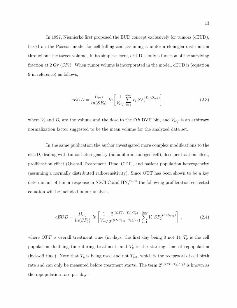
In 1997, Niemierko first proposed the EUD concept exclusively for tumors (cEUD),

based on the Poisson model for cell killing and assuming a uniform clonogen distribution

throughout the target volume. In its simplest form, cEUD is only a function of the surviving

fraction at 2 Gy (SF2). When tumor volume is incorporated in the model, cEUD is (equation

9 in reference) as follows,

cEUD = Dref

ln(SF2)ln

C1

Vref

binsÿ

i=1Vi SF

(Di/Dref )2

D

. (2.3)

where Vi and Di are the volume and the dose to the iÕth DVH bin, and Vref is an arbitrary

normalization factor suggested to be the mean volume for the analyzed data set.

In the same publication the author investigated more complex modifications to the

cEUD, dealing with tumor heterogeneity (nonuniform clonogen cell), dose per fraction e�ect,

proliferation e�ect (Overall Treatement Time, OTT), and patient population heterogeneity

(assuming a normally distributed radiosensitivity). Since OTT has been shown to be a key

determinant of tumor response in NSCLC and HN,29–32 the following profileration corrected

equation will be included in our analysis:

cEUD = Dref

ln(SF2)ln

C1

Vref

2((OT Ti≠Tk)/Tp)

2((OT Tref ≠Tk)/Tp)binsÿ

i=1Vi SF

(Di/Dref )2

D

. (2.4)

where OTT is overall treatment time (in days, the first day being 0 not 1), Tp is the cell

population doubling time during treatment, and Tk is the starting time of repopulation

(kick-o� time). Note that Tp is being used and not Tpot, which is the reciprocal of cell birth

rate and can only be measured before treatment starts. The term 2((OT T ≠Tk)/Tp) is known as

the repopulation rate per day.

14

In 1999, Niemierko proposed a unified phenomenological model applicable to both

tumor and normal tissues, known as the generalized-EUD (gEUD).33 gEUD uses a power-

law which is a generalized mean or power mean of the dose in each voxel of volume, as in

Equation 2.5. The exponent, a, is determined from numerical fits to clinical data and vi

is the fraction of volume in the iÕth tumor voxel. When assessing dose distributions within

normal tissues, a falls between 0 and 1. For tumors it is believed to range from -1 and

-20.34

gEUD =C

binsÿ

i=1vi Da

i

D1/a

. (2.5)

Uniformly distributed doses have been shown to give the highest local control,35

for this reason EUD formulations have been used to assess LC. gEUD has so far been used

to compare treatment plans,36 as an optimization parameter in treatment34,37,38 and it is

directly correlated with late toxicity in outcome analysis.39 However, reported correlations

with LC have not been conclusive.

On the other hand, cEUD has been ‘little-studied’. To date, it registers some

treatment plan comparisons40–42 and only three outcome analysis studies. Levegrun et al.

made use of the simplest formulation over the planning target volume (PTV) in prostate

cancer reporting the same level of correlation as for the median dose.43 Terahara et al.

included volume e�ect in the GTV for skull base chordoma, reporting good correlations.44

The third study makes reference to cEUD, however it does not report any SF2 value nor

any other variable they might be using for cEUD computation.45

15

2.5 Setup errors

Patient setup error is defined as the di�erence between the intended and the actual position

of the patient.46 Generally, setup errors are divided into random or interfractional errors

(deviations between di�erent fractions/daily fluctuations) and systematic errors (patient

is set up using incorrect positioning information). Immobilization devices have improved

treatment delivery accuracy (see Figures 2.4 for examples); but, since the imaging device

and correction procedure have finite accuracy, there will always be residual error.

In order to account for setup errors safety margins are created around the target

volumes. This safety margin minimizes the risk of tumor geometrical misses. ICRU Reports

50 and 6247,48 define the relevant terminology. First, the gross tumor volume (GTV) is

defined as the volume containing visible tumor on the diagnostic images. Second, the clinical

target volume (CTV) is defined to enclose the GTV plus a margin to account for possible

sub-clinical disease. The planning target volume (PTV) is defined by the CTV plus a margin

to allow for geometrical variation such as patient movement, set-up uncertainty and organ

motion. Figure 2.5 below explains schematically the relationship between these volumes.

This margin is defined by two components: (a) internal margin (IM) to account for variation

in size, shape, and position of CTV, and (b) setup margin (SM) to account for uncertainties

in patient position and beam alignment. The choice of the size of margins is usually based

on clinical experience and should include all the e�ects that contribute to the uncertainty

in position of the CTV, including inter-fraction and intra-fraction variations. Appropriate

imaging is therefore highly relevant in the determination of the PTV. The inter-fraction and

intra-fraction factors included in the PTV are based on population studies using imaging

modalities.

16

(a) Thermoplastic mask used for immobilization dur-ing head and neck treatment. Picture taken fromwww.bionixrt.com

(b) Vaclock or polyurethane foam cast, used for3DCRT lung cancer treatment. Figure taken fromwww.alphacradle.com

Figure 2.4: Example of immobilization device for head and neck and lung cancer treatment.

17

Figure 2.5: Scheme of ICRU definitions of di�erent treatment target volumes (Gross, ClinicalInternal and Planning Target Volumes), including internal margin (IM) and setup margin(SM). Figure taken from ICRU 62.

Treatment planning studies have been made to quantify setup errors, and define

margin sizes for various anatomical sites and method of immobilization.49,50 In HN, 3 to

5 mm margins are believed to be adequate to compensate for setup uncertainties.40 In lung

cancer, only the random errors are as high as 6 mm49 and are on the order of a centimeter

or more in the superior-inferior direction.51 Lung tumors positional o�sets are also more

complicated to study because the uncertainty nature is not totally random; there is a pattern

due to respiratory motion making di�cult to predict as there is a variation among patients.52

Breathholds or shallow breathing, respiratory gating, and synchronized techniques are among

the tools currently used to counter this issue.53 These approaches merely provide a beam-on

sequence and reduce patient/tumor motion. Thus the uncertainty, even though reduced,

persists.

18

2.6 Biologically based treatment planning

Until recently, the quality of a RT plan has been evaluated by dose distributions and dose-

volume (DV) quantities, thought to correlate with biological responses (normal tissue com-

plications and tumor control). It is widely accepted that the DV criteria, which may be

considered a surrogate of biological responses, should be replaced by biological indices in

order to more closely reflect clinical goals of RT.54

Radiobiological models estimate tumor local control probability (TCP) and normal

tissue complication probability (NTCP). These models have also been used to retrospectively

correlate plan’s dosimetric or patient’s clinical characteristics to learn how to improve TCP

or/and NTCP. Lately, they have been used to evaluate radiotherapy treatment plans, so

they can be compared.

Dose-response models for tumor and normal structures can be roughly categorized

as either mechanistic or phenomenological. Mechanistic models attempt to mathematically

formulate the underlying biological processes, whereas the latter simply intend to fit the

available data empirically.

Mechanistic models are often considered preferable, as they may be more rigorous

and scientifically sound. However, the underlying biological processes for most tumor and

normal tissue responses are fairly complex. Because of this complexity, mechanistic models

often are not fully understood, making not feasible to completely describe the phenomena

mathematically.

On the other hand, phenomenological models are advantageous since they typically

are relatively simple compared to the mechanistic models. Their use avoids the need to fully

understand the underlying biological phenomena. A limitation of these models may arise

19

from temptation to simplify in excess the model and thus limit their ability to consider more

complex phenomena.

Although absolute values of predicted outcome probabilities may not yet be reliable

because of lack of validation studies, such tools might provide useful information when

alternate treatment plans are compared, particularly in cases where dosimetric advantages

of one plan over another is not clear-cut according to DV criteria. Biological optimization

for radiotherapy may be the way forward for improving treatment outcomes.

Next Chapter studies LC correlation with all available parameters (clinical and

dosimetric) in order to demonstrate that the gDT formulation, proposed by this dissertation,

performs the best in HN and NSCLC cohorts.

20

Chapter 3

Local Control correlation

3.1 Introduction

In this chapter all available clinical and dosimetric characteristics of the patient cohorts will

be studied for correlation with local control, including EUD formulations. The objective is

to find the best available model that predicts LC to then compare it with the novel model

that this dissertation proposes.

A very important characteristic of predictive models used in clinical practice, is that

they should be easy to use, implement and adapt to your daily work. For this reason, the

purpose of this study was to find a powerful yet simple model. Even though more complex

analyses will construct more representative models of the datasets, they will also be more

complex to implement and use on a daily basis.

The simplest form of quantitative statistical analysis is the so called univariate

analysis. This analysis explores each variable in a data set independently. It looks at the

range of values, as well as the central tendency of them, and it describes the pattern of

21

response to a variable. Univariate and multivariate of several di�erent orders analysis were

used to study LC correlation.

3.2 Materials and methods

3.2.1 Patient cohorts

Two retrospectively collected datasets of patients treated at Washington University in Saint

Louis were compiled for LC assessment, named "HN" and "NSCLC" cohorts.

NSCLC cohort

The lung cancer dataset consisted of 157 consecutive patients with NSCLC treated between

1991 and 2001 using three-dimensional conformal radiation therapy (3DCRT), see Figure 3.1

for an example of the dose distributions. Of these, only 56 patients had a primary isolated

lesion and entered to this analysis. They were treated to a prescribed dose between 50 and 90

Gy, and standard fractionation for NSCLC which ranged between 1.8-2.2 Gy/day. Isolated

lesions with local control status were determined radiographically on follow-up. Patients

were considered to have local control of disease if they had an initial radiographic response

on CT images to treatment and a stable mass (also referred to as ‘progression free’ ) at

each follow-up visit. Otherwise, patients were considered to have local failure if clinical,

radiographic, or biopsy evidence of progression was observed. A minimum follow-up of 6

months was used. From the 56 patients left out for analysis, 22 patients presented primary

tumor (GTV-T) recurrence during follow-up. Median follow-up time for all patients was 20

months, ranging from 1 to 74 months. Monte Carlo-corrected dose distributions were used

for the analysis.55

22

Figure 3.1: An example of non small cell lung treatment dose distributions of this cohort.

HN cohort

Between 1998 and 2008, 162 consecutive patients with HN squamous cell carcinoma exclusive

of the nasopharynx, paranasal sinuses, and salivary glands were treated definitively with

IMRT. 72 of these patients had induction chemotherapy and were not analyzed, and 10

had unrecoverable data. The 80 patients left for analysis had been treated with IMRT to

a median dose of 70 Gy with standard fractionation of 2 Gy per fraction, Figure 3.2 shows

an example of the dose distributions from this dataset. Out of these 80 patients, 23 had

local failure (GTV-T recurrence). The median follow-up time was 19 months with a range

of 2-137 months.

Patient data extraction was made using open-source software called CERR (compu-

tational environment for radiotherapy research) which allows for fast, e�cient and accurate

23

Figure 3.2: An example of head and neck dose distributions of this cohort.

extraction of a wide range of treatment plan characteristics.56 This tool is built in MATLAB

(MathWorks, Natick, MA) which was used for all data analysis in this dissertation.

3.2.2 Analysis

3.2.2.1 Variables

Since our objective is to assess local control only, all dose analysis was done for the primary

tumor (GTV-T) only, excluding distant disease or lymph node involvement. This means

that the minimum dose, for instance, to the GTV-T and not to the CTV nor PTV was

extracted. The dose-volume parameters examined were: minimum dose, maximum dose,

mean dose, D5 to D95 (where Dx is the minimum dose given to the hottest x% volume), V5

to V80 (where Vx represents the percentage volume that receives greater or equal x dose).

24

gEUD for di�erent values of the exponent ‘a’ and cEUD for di�erent values of the surviving

fraction at 2 Gy (SF2), were also evaluated. Additional analyzed prognostic factors include

age, sex, race, T-stage, N-stage, stage group, chemotherapy, and tumor volume. Tumor

volume was calculated based on the size of the GTV-T in the pretreatment (simulation) CT

image.

3.2.2.2 Model building and assessment

The first step to take in predictive model construction is to study models built on univariate

analysis. This is because of the simplicity of the model construction and it’s straightforward

application. All variables named on the previous subsection were assessed using univariate

analysis. Correlation with LC was quantified using the area under the receiver operating

characteristic (ROC) curve and Spearman’s rank correlation coe�cient (Rs) with its re-

spective p-value. The Spearman correlation was chosen because it is less sensitive than the

Pearson correlation to strong outliers that are in the tails of the samples.57 This is because

Spearman’s Rs limits the outlier to the value of its rank. The ROC curve, Figure 3.3, plots

the tradeo� between sensitivity (fraction of people with LC correctly identified as positive

by the model) and specificity (fraction of people without LC correctly identified as negative

by the model) and shows the performance of a binary classifier. The area under this curve

(AUC) is a measure of the classification accuracy. An AUC of 0.5 means that the model does

not perform better than random guess, and an AUC of 1 reflects the perfect model.

Dose response curves were built using logistic regression model which also provides

an estimation of the probability PLC of observing LC. The regression model is given by:

PLC = exp(b0 + b1x1 + · · · + bnxn)1 + exp(b0 + b1x1 + · · · + bnxn) . (3.1)

25

Figure 3.3: The receiver operating characteristic (ROC) curve. The dotted line shown inthe ROC curve represents a useless test that has no discriminatory power.

where x1,. . . , xn is the set of n variables examined, and b0, b1,. . . , bn is the set of (n + 1)

logistic model coe�cients to be fitted.

3.2.2.3 Model robusteness

The ability of any model to correctly predict outcome should ideally be tested on an in-

dependent group of patients with similar treatment characteristics. Because such datasets

most of the time are not easily available, it may then be possible to internally validate the

model. The most accepted methods for obtaining a good internal validation of a model’s per-

formance are data-splitting, repeated data-splitting, jackknife technique and bootstrapping

cross-validation (CV). We use two di�erent cross-validation methods, the bootstrap and the

10-Fold CV. With the bootstrap method, the model is applied to a large number ( 10,000) of

random permutations of the outcome data. 10-Fold CV consists of partitioning the dataset

26

in 10 subsets; then, build the model on 9 of this subsets and calculate the probability of

observing LC for the subset left out.

3.2.2.4 Kaplan-Meier estimates

In order to find a low-high risk group di�erentiation to be used clinically, actuarial local

control analysis was carried out using the resultant most predictive parameter.58 The event

scored is local progression in NSCLC, or local recurrence in HN, of the primary tumor.

Starting from the first day of treatment, patients are censored at the time of their last follow-

up or local failure. The log-rank method is used to assess group di�erence significance.

3.3 Univariate local control prediction results

3.3.1 Vx

and Dx

parameters

All the available clinical and dose-volume parameters were evaluated independently for cor-

relations with LC. Dx and Vx univariate analysis results are summarized in Figures 3.4 and

3.5, for the HN and NSCLC cohorts respectively.

We can observe that in HN, V70 is the only parameter significantly correlated with

LC among all Vxs (AUC = 0.6716; Rs = 0.2765; p = 0.007). 70 Gy has been found to be a

good dose prescription to cure HN cancers,59 therefore it is not a surprise that the volume

receiving the prescription dose is correlated with LC. Among all Dxs, D80 and above predict

LC, being the more correlated D100, which is the minimum dose (AUC = 0.6895; Rs =

0.2973; p = 0.004).

For NSCLC, V75 and V80 are both found to be significantly correlated to LC, with

V75 being the best predictor (AUC = 0.6638; Rs = 0.2943; p = 0.015). Even though dose

27

Figure 3.4: Correlation results for V5 to V80 and D5 to D100 parameters of the Head andNeck. Dotted line indicates statistically significant threshold (0.05).

28

prescriptions range over a wide window (between 50 and 90 Gy), the mean dose prescription

it is smaller than 70 Gy. For this reason it is very curious that the volume receiving doses

from 75 Gy (high doses compared to the mean) shows the best correlation with LC. I said

curious because it might be suggesting that doses higher that the current prescriptions are

needed to e�ectively control the tumor.17,18

Several Dxs below D65 passed the significance test, with D40 having best corre-

lation to LC (AUC = 0.6638; Rs = 0.2771; p = 0.02). These correlations, however, are

not very powerful and when tested on cross-validation do not remain significant in either

dataset.

3.3.2 All other parameters

Tables 3.1 and 3.2 summarize the results for the univariate analysis for the HN and NSCLC

cohorts respectively. Tumor volume was one of the most significantly correlated parameters

with LC for both datasets. The maximum dose did not show significant correlation with LC

in either dataset (p = 0.4 and 0.1 in HN and NSCLC, respectively). The mean dose appeared

non-predictive in HN (p = 0.2), whereas the minimum dose did not pass the significance

threshold in NSCLC (p = 0.07). gEUD did not correlate with LC in HN, showing the least

poor result (p = 0.15) at a = -4, although it showed significance for NSCLC. The simplest

cEUD formulation which is tumor volume independent had no predictive power for this HN

dataset scoring at best p = 0.06 when SF2 = 0.1. However, the volume corrected cEUD

formulation, Equation 4.1, was the most predictive variable at SF2 = 0.8 for both, HN and

NSCLC.

Table 3.3 shows which variables are statistically significant on univariate analysis

for both datasets. PASS means that the parameter correlates significantly with LC at the

p-value<0.05 threshold, and FAIL states the opposite. It can be observed that there are

29

Figure 3.5: Correlation results for V5 to V80 and D5 to D100 parameters in NSCLC. Dottedline indicates statistically significant threshold (0.05).

30

Table 3.1: Statistically significant parameters and their correlation rank coe�cients on uni-variate analysis for head and neck cohort.

parameters AUC Rs p-value

Stage group 0.6392 0.2934 0.0051T-stage 0.6842 0.2988 0.004 1Volume 0.7544 0.3989 0.0002Minimum dose 0.6895 0.2973 0.004V70 0.672 0.277 0.007cEUD 0.7834 0.4443 0.00004

Rank coe�cients are shown for significant parameters at the 0.05 level only.

Table 3.2: Statistically significant parameters and their correlation rank coe�cients on uni-variate analysis for NSCLC cohort.

parameters AUC Rs p-value

T-stage 0.6330 0.2516 0.031Age 0.6544 0.2617 0.026Volume 0.7420 0.4094 0.002Mean dose 0.6497 0.253 0.030D35 0.664 0.277 0.02V75 0.664 0.294 0.015gEUD 0.6471 0.2488 0.032cEUD 0.7607 0.4411 0.001

Rank coe�cients are shown for significant parameters at the 0.05 level only. a Volumecorrected cEUD.

31

Table 3.3: Comparison of statistically significant parameters on univariate analysis for bothdatasets.

parameters HN NSCLC

Stage group PASS FAILT-stage PASS PASSAge FAIL PASSVolume PASS PASSMinimum dose PASS FAILMean dose FAIL PASSD35 FAIL PASSV70 PASS FAILV75 FAIL PASSgEUD FAIL PASScEUD PASS PASS

only three parameters that correlate with LC in both datasets: T-stage, tumor volume, and

cEUD volume corrected. It could be said that, somehow, all three parameters contain tumor

volume.

When testing our parameters on 10-fold cross-validation we found out that the

only parameters that remain statistically significant are volume and cEUD for both data

sets. Robustness performance results are shown in Table 3.4, where cEUD volume corrected

method performed the best once again. These findings suggest cEUD is a robust predictor

of local control.

3.3.3 Multivariate analysis

Two and higher order multivariate models were built using all possible combination of all

available parameters. Even though more complex model constructions will be more rep-

resentative of the dataset, since this higher order models take more degrees of freedom as

32

Table 3.4: Summary of Statistically significant model parameters results on univariate anal-ysis after performing cross-validation.

HN NSCLC

parameters AUC Rs p-value AUC Rs p-value

Volume 0.6984 0.3111 0.005 0.6656 0.2801 0.03cEUD 0.7575 0.4037 0.0002 0.7272 0.3845 0.003

well, after cross-validation they lose their predictive power. Our analysis showed that a two

parameter, cEUD volume corrected and stage group, model was the most significant when

cross-validated for HN only (RsCV=0.4644, pCV-value=0.02). The same model was not

a good predictor of LC for the NSCLC cohort. Higher order models did not appear more

predictive than the cEUD univariate model after cross-validation for either dataset.

3.3.4 EUDs

Based on these results we decided to take a closer look at the cEUD volume corrected as

defined in Equation 4.1 and the gEUD formula Equation 2.5. We investigated the cEUD

correlation dependency on SF2 and Vref , as well as the e�ect of the exponent a for the gEUD.

Influence of SF2 and a parameters in the correlation of the respective EUDs is plotted in

Figure 3.6. We can see that cEUD, not including the volume e�ect, and the gEUD, with a

varying from -1 to -20, performed almost evenly. On the other hand, we can observe that

the volume corrected cEUD is outstandingly better correlated at any given value of SF2.

For this reason, from here after, we will focus on the volume corrected cEUD only.

The best performance for both datasets is obtained for cEUD at SF2 = 0.8 (as

reported in Table 3.4). Considering SF2 = 0.5 in the calculation of cEUD we obtained

Rs=0.4096, p-value«0.05, and AUC=0.761; which still performed better than other parame-

33

ters. The correlation of cEUD with LC deteriorates for decreasing values of SF2. Despite the

better correlation of cEUD for large SF2 values, we do not think it reflects the underlying

radiobiology.

cEUD correlation with LC showed to be independent of the Vref parameter in

Equation 4.1. We vary Vref between 10≠6 and 10+4 obtaining always the same correlation

results i.e. the same Rs, AUC and p-values, as shown in Figure 3.7. Vref plays a cEUD-

normalization roll only, the higher the Vref the higher the cEUD.

Although Niemierko suggested setting Vref equal to the median volume, we hypoth-

esize that a more adequate Vref selection could help di�erentiate low from high risk groups.

Here, we set Vref to 14 cc because correspond to a sphere of 3 cm which is the maximum

diameter for a T1 stage tumor in NSCLC. Although that is not true in HN, we used the

same Vref . We will further investigate the reference volume in order to test our hypothesis

and thus, perhaps, depict in a more adequate manner the dataset that is representing.

Figure 3.8 below plots the logistic regression model (circles) of cEUD for SF2 = 0.8

for both data sets; squares represent the binned observed rates of local control, error bars

represent estimated binomial confidence interval (CI) in each given bin; and red dashed lines

represent the 95% CI for the logistic regression. We can see that the dose curve for NSCLC

is less steep and covers a wider range of cEUD values than in HN. It can also be said that

in both cases data and prediction follow closely.

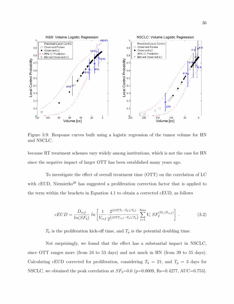
Figure 3.9 represents, in the the same graph type, the logistic regression model

based on tumor volume. We observe higher local control rates with decreasing tumor volume,

as expected. This e�ect is more obvious in the NSCLC cohort. However, in both cases the

response curve does not get the "S" shape that, at least theoretically, should have.

Overall treatment time (OTT) has been shown to be a key determinant of tumor

response in NSCLC.29–32 This may become an issue when studying local control in NSCLC

34

Figure 3.6: Dependency of the EUDs on their respective parameters.

35

Figure 3.7: cEUD dependency on di�erent Vref values.

Figure 3.8: Dose response curves built using a logistic regression of the cEUD for HN andNSCLC.

36

Figure 3.9: Response curves built using a logistic regression of the tumor volume for HNand NSCLC.

because RT treatment schemes vary widely among institutions, which is not the case for HN

since the negative impact of larger OTT has been established many years ago.

To investigate the e�ect of overall treatment time (OTT) on the correlation of LC

with cEUD, Niemierko28 has suggested a proliferation correction factor that is applied to

the term within the brackets in Equation 4.1 to obtain a corrected cEUD, as follows

cEUD = Dref

ln(SF2)ln

C1

Vref

2((OT Ti≠Tk)/Tp)

2((OT Tref ≠Tk)/Tp)binsÿ

i=1Vi SF

(Di/Dref )2

D

. (3.2)

Tk is the proliferation kick-o� time, and Tp is the potential doubling time.

Not surprisingly, we found that the e�ect has a substantial impact in NSCLC,

since OTT ranges more (from 24 to 53 days) and not much in HN (from 39 to 55 days).

Calculating cEUD corrected for proliferation, considering Tk = 21; and Tp = 3 days for

NSCLC, we obtained the peak correlation at SF2=0.6 (p=0.0009, Rs=0.4277, AUC=0.753).

37

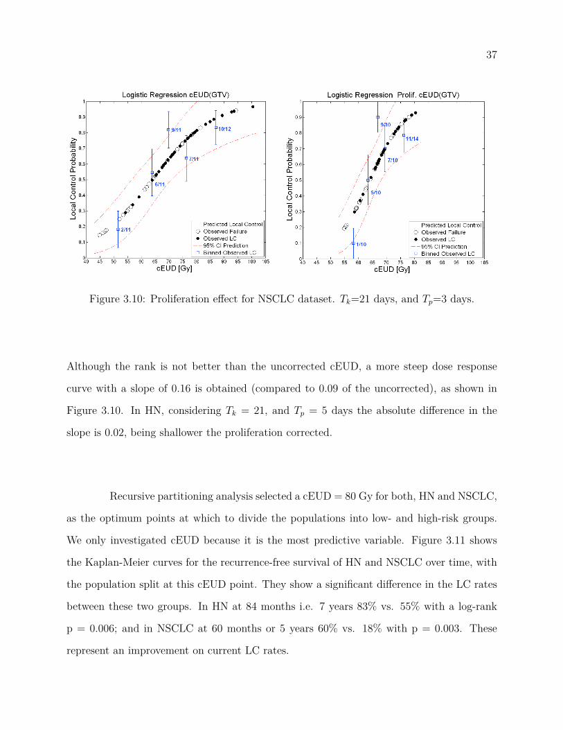
Figure 3.10: Proliferation e�ect for NSCLC dataset. Tk=21 days, and Tp=3 days.

Although the rank is not better than the uncorrected cEUD, a more steep dose response

curve with a slope of 0.16 is obtained (compared to 0.09 of the uncorrected), as shown in

Figure 3.10. In HN, considering Tk = 21, and Tp = 5 days the absolute di�erence in the

slope is 0.02, being shallower the proliferation corrected.

Recursive partitioning analysis selected a cEUD = 80 Gy for both, HN and NSCLC,

as the optimum points at which to divide the populations into low- and high-risk groups.

We only investigated cEUD because it is the most predictive variable. Figure 3.11 shows

the Kaplan-Meier curves for the recurrence-free survival of HN and NSCLC over time, with

the population split at this cEUD point. They show a significant di�erence in the LC rates

between these two groups. In HN at 84 months i.e. 7 years 83% vs. 55% with a log-rank

p = 0.006; and in NSCLC at 60 months or 5 years 60% vs. 18% with p = 0.003. These

represent an improvement on current LC rates.

38

Figure 3.11: Actuarial estimates for HN and NSCLC based on cEUD cuto�s.

3.4 Discussion

Several dosimetric and clinical factors, including equivalent uniform dose formulations were

analyzed to rank local control in head and neck and non-small-cell lung cancers. The cell-kill

based EUD (volume corrected) showed to be a simple and useful parameter when predicting

local control in these two datasets, having the highest correlation. The best-fit was found at

high SF2 values (0.8). It is di�cult to believe such high radioresistance value is representative

of the underlying radiobiology since many in vitro studies have shown di�erently. Therefore,

a deeper study of this seemingly high radioresistance needs to be done.

When investigated the e�ect of overall treatment time (OTT) on local control, not

surprisingly, the e�ect was seen in this NSCLC cohort. Accounting for this e�ect in lung

resulted in a more representative dose response curve, and a lower SF2 fraction, though still

high (SF2 = 0.6). The same e�ect could not be seen in the HN cohort since OTT throughout

patients was nearly the same.

39

It was demonstrated here, as previous publications suggested, that tumor volume

does play a very important role at predicting local control.20–23 This is evidenced by the fact

that the cEUD formulation that includes the absolute volume e�ect results in the highest

correlated single parameter with LC.

Recursive partitioning analysis showed an important increase in recurrence-free

survival for NSCLC (figure 3.11), at a dose cut-o� of 80 Gy which is much higher than the

typical 3DCRT prescription doses (about 60 Gy). Although this high prescription dose is not

practicable in 3DCRT due to the high radiosensitivity of the lungs (the normal surrounding

tissue), it might give the foundation for SBRT treatment. So, yet another way to test our

results in lung cancer will be to analyze SBRT cases, where local control rates are very good.

Hence, it remains to be studied whether local control predictions can be done according

to the same parameters in patients treated with short, hypofractionated treatments. The

overall conclusion is that cEUD may be a simple and useful metric for treatment plan decision

support, but needs further testing on clinical data.

In the following chapter, modifications to cEUD and a newly proposed EUD for-

mulation will be studied for correlation with LC to seek for consistency with already known

radiosensitivity values. The predictive power of these formulations will be compared to

cEUD performance in order to establish their further usefulness.

40

Chapter 4

cEUD modifications and generalized

tumor dose (gTD) formulation

4.1 Introduction

The cEUD formula, which accounts for varying tumor volume as well as dose variability in

the tumor, has been shown to be highly correlated with local control in HN and NSCLC

tumor datasets, as demonstrated in Chapter 3. However, previous fits resulted in high

surviving fractions at 2 Gy (SF2 0.8) which is contrary to radiobiologically observed in

vitro studies.

This chapter presents a novel modification to the cEUD equation in order to obtain

a more realistic model the in terms of already published radiosensitivity values, while trying

to keep previous models performance.

In addition, a new equivalent uniform dose formulation named generalized tumor

dose (gTD) is introduced. This formulation is designed for tumors only and takes a form

41

similar to a power or generalized mean. Moreover, the proposed formulation is, as well as

other EUD formulations, easily implementable in a routine clinical practice.

4.2 Modified SF2

A modification of the surviving fraction at 2 Gy (SF2) to be applied to the cell-kill-based

equivalent uniform dose (cEUD) published by Niemierko28 is proposed. This change allows a

high correlation between local control (LC) and cEUD while using a radiobiologically correct

SF2 value. The cEUD equation used is presented in chapter 2, but in order to facilitate the

reader’s comprehension it is repeated here,

cEUD = Dref

ln(SF2)ln

C1

Vref

binsÿ

i=1Vi SF

(Di/Dref )2

D

. (4.1)

We calculated the cEUD according to Equation 4.1 for the HN and NSCLC datasets

described in Chapter 3, for di�erent values of the unknown SF2 fraction. Here, Dref is 2 Gy

and Vref is arbitrarily chosen to be 14 cc, Vref plays a normalization role only (the higher

Vref the higher cEUD, and the correlation with LC is independent of it). We obtained the

highest correlation for both datasets when setting SF2 at 0.8, and decreasing correlation

with lower SF2. However, SF2= 0.8 is too high to be radiobiologically plausible.

For this reason this dissertation proposes to replace SF2 in Equation 4.1 with

an e�ective SF2, which takes into account the increasing radioresistance we observed, also

based on the well known fact that the surviving fraction is proportional to the tumor vol-

ume. Therefore, introducing the increase as function of the tumor volume, the modification

proposed is as follows:

42

SF2 effective = SF2

A

1 + kVT

Vref

B

(4.2)

and thus,

cEUDÕ = Dref

lnËSF2

11 + k VT

Vref

2È ln

C1

Vref

binsÿ

i=1Vi [SF2

A

1 + kVT

Vref

B

](Di/Dref )D

. (4.3)

where Vref is the same arbitrary variable as in Equation 4.1, VT is the absolute tumor volume,

and k is a constant of proportionality to be determined using outcome data.

The discriminative abilities of the model and accuracy at correlating LC were tested

using the area under the receiver operating characteristic curve AUC (i.e. the agreement

between predicted and observed outcome). An AUC of 0.5 means that the model does not

perform better than random guess, and an AUC of 1 reflects the perfect model.

The results of the correlation of LC with cEUD using the modified SF2 are shown

in the Figure 4.1. Maps of the AUC values for di�erent SF2 and k values are plotted for

both datasets. Dark red areas represent the higher correlation with local control, and dark

blue represents the least correlated pair of parameters. We can observe that for k = 0.05

we obtained SF2 estimates radiobiologically meaningful while keeping a high correlation (at

dashed lines, AUC= 0.729 for lung and AUC = 0.758 for HN), although it does not represent

the highest correlation. Moreover, AUC values did not significantly increased compared to

the uncorrected model.

Figure 4.2 depicts the logistic regression model (circles) of cEUD with the e�ective

SF2 for both data sets using the best fit parameters; squares represent the binned observed

43

Figure 4.1: Maps of the AUC values for di�erent SF2 and k values for both datasets. Dashedlines intersection represents a high correlation while keeping a radiobiologically meaningfulSF2 value.

rates of local control, error bars represent estimated binomial confidence interval (CI) in

each given bin; and red dashed lines represent the 95% CI for the logistic regression.

If we compare these curves with the ones for the uncorrected cEUD (figure 3.8), we

can observe that: a) the HN dose response curve is shallower than before; b) failures are not

distinguishably grouped at the low dose part of the curve, which means a poor specificity

and sensitivity; c) NSCLC dose response curve has a longer lower tail than before; and d)

in HN and NSCLC cases data are not as well fitted as for the uncorrected cEUD.

From these results it can be concluded that, even by introducing a modification to

the cEUD formulation to make it agree with already tested radiobiological parameters, we

lose predictive power, and worse, the cEUD tends to keep preferring high – values. This is

why a new uniform dose formulation will be presented in the following section.

44

Figure 4.2: Dose response curves built using a logistic regression of the cEUD with thee�ective SF2 for HN and NSCLC.

4.3 Generalized Tumor Dose (gTD) formulation

Neimeirko’s generalized equivalent dose concept for tumors is based on the Poisson model

for cell killing and assumes an uniform clonogen distribution throughout the target volume,

as detailed in Section 2.4. The same author proposed a unified phenomenological model

applicable to both tumor and normal tissues, known as the generalized-EUD (gEUD).33

gEUD uses a power-law which is a generalized mean or power mean. The exponent, a, is

determined from numerical fits to clinical data. It is a widely cited formula that has seldom

been fit to actual tumor response data.

Because a key determinant of tumor response is tumor volume, this dissertation

constructs a new concept of equivalent uniform dose that includes the e�ect of absolute tumor

volume, just as proposed previously by Niemierko (Equation 4.1), but also introducing a

parameterization that weights cell kill in the hottest or coldest regions of a tumor. The result

is a simple metric of tumor dose distribution quality that is of the form of the generalized

45

mean of the dose that the primary tumor receives, which is termed generalized tumor dose

or gTD.

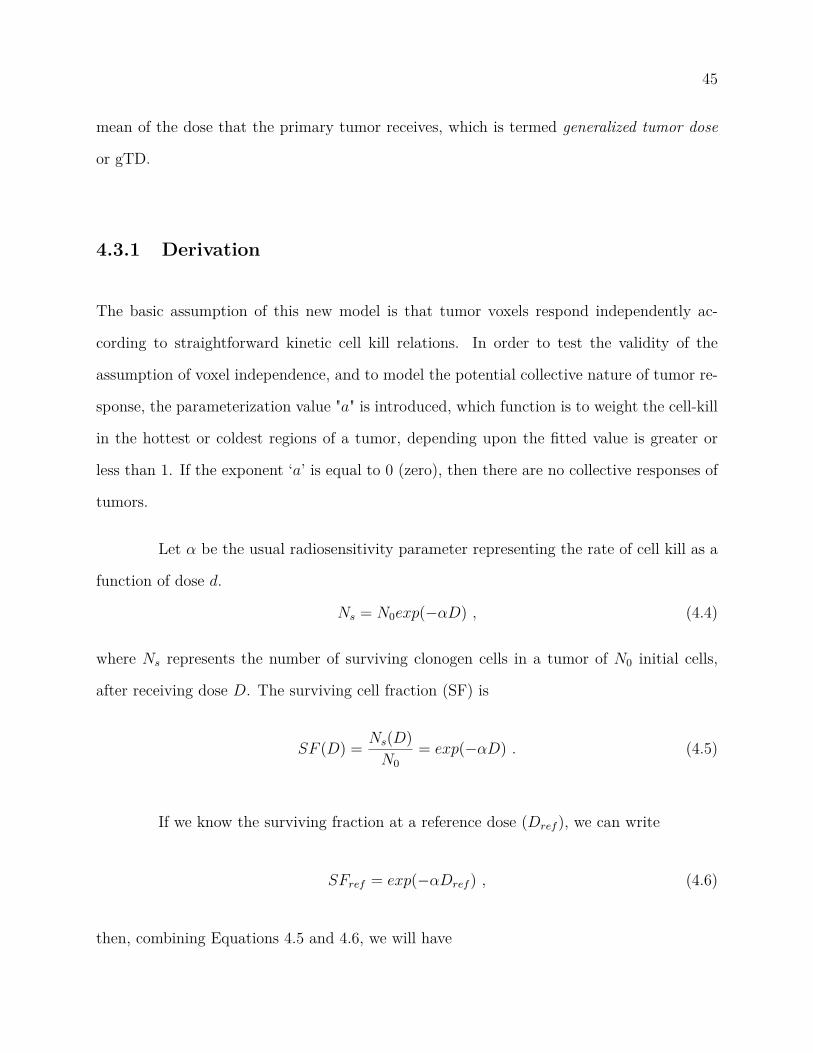
4.3.1 Derivation

The basic assumption of this new model is that tumor voxels respond independently ac-

cording to straightforward kinetic cell kill relations. In order to test the validity of the

assumption of voxel independence, and to model the potential collective nature of tumor re-

sponse, the parameterization value "a" is introduced, which function is to weight the cell-kill

in the hottest or coldest regions of a tumor, depending upon the fitted value is greater or

less than 1. If the exponent ‘a’ is equal to 0 (zero), then there are no collective responses of

tumors.

Let – be the usual radiosensitivity parameter representing the rate of cell kill as a

function of dose d.

Ns = N0exp(≠–D) , (4.4)

where Ns represents the number of surviving clonogen cells in a tumor of N0 initial cells,

after receiving dose D. The surviving cell fraction (SF) is

SF (D) = Ns(D)N0

= exp(≠–D) . (4.5)

If we know the surviving fraction at a reference dose (Dref ), we can write

SFref = exp(≠–Dref ) , (4.6)

then, combining Equations 4.5 and 4.6, we will have

46

SF (D) = SF(D/Dref )ref . (4.7)

Assuming cells are uniformly distributed throughout the tumor volume, the total

SF can be written as:

SF (EUD) =Lÿ

i=1wiSF (Di) . (4.8)

On the other hand, we can also assume that the number of surviving cells is directly

proportional to the tumor volume and that the constant of proportionality c is tumor volume

independent,20 thus we have:

wi = c Vi ; (4.9)

and

SF (EUD) = cLÿ

i=1ViSF (Di) , (4.10)

or

exp(≠–EUD) = cLÿ

i=1ViSF (Di) . (4.11)

Taking the natural logarithm and dividing by ≠– written in terms of Dref and SFref , we

obtain

EUD = Dref

ln(SF2)ln

C

cLÿ

i=1ViSF (Di)

D

, (4.12)

since wi is dimensionless, the constant of proportionality c must have units of 1/volume.

Here we introduce the generalized mean parameter to model the potential collective

response of tumors. This is done by taking the generalized mean of the voxel cell survival

probabilities. The resulting dose is denoted the generalized tumor dose, or gTD:

47

gTD = Dref

ln(SF2)ln

C1

Vref

binsÿ

i=1Vi SF

(a Di/Dref )2

D1/a

. (4.13)

From this we can see that introducing collective e�ects through this modeling mech-

anism has the e�ect of de-coupling the impact of tumor volume (the first term) from cell

survival (the second term.)

The role of a as a fitting parameter will specifically be to define whether the high-

dose regions are more influential (a < 1), or if the low dose regions are more influential

(a > 1).

Applying the linear quadratic model, we can write,

gTD = ≠1– + Dref—

ln

C1

Vref

binsÿ

i=1Vi exp(≠–Di ≠ —DiDref )a

D1/a

. (4.14)

Although more complex formulations are possible, the simplicity of the model is

attractive since it is an important criteria in developing clinically useful models. Like the cell-

kill-based EUD, it has the advantage that we do not need to know the (typically unknown)

clonogen density. Moreover, it has the desired property that tumors of varying volumes are

naturally handled without the introduction of any new parameters.

Implementation of the gTD was made in MATLAB. Appendix A contains the entire

MATLAB file with this implementation.

4.3.2 Parameter fitting methods

Performance of an outcome prediction model can be judged in several ways using a variety

of parametric and nonparametric goodness-of-fit tests such as the Chi-square statistic, cor-

48

relation coe�cients, and receiver operating characteristic curves.57 However, when fitting a

parameter of a function given an outcome, the likelihood is the optimization of choice.

The likelihood (denoted L) of generating the observed data given a model that

predicts tumor control probability (TCP) is:

L =LCŸ

TCP ◊LFŸ

(1-TCP),

where LC represents cases where local (gross disease) control was observed at last followup,

and LF represents local failures at last followup. Here, control really refers to a lack of

evidence of growth, since the tumor typically does not shrink completely away.

A more convenient form of the likelihood is to take the logarithm (called the log-

likelihood, denoted LL), which is helpful for numerical reasons as well, since all data points

will contribute significantly to the resulting sum:

LL =LCÿ

log(TCP) +LFÿ

log(1-TCP).

In our case we adopt a simple parameterization of the dose-response curve:

TCP = exp(x)1 + exp(x) ,

where x = b0 + b1 ◊ gTD. This has the same form of a logistic regression (Equation 3.1).

The exponent a is the model parameter that is determined by maximizing the probability

that the data gave rise to the observations.

49

Figure 4.3: Generalized tumor dose (gTD) dependency on its two variables (– and a) forhead and neck and NSCLC.

4.3.3 Results of gTD fitted to clinical outcome data

We calculated the gTD according to Equation 6.1 for the HN and NSCLC datasets described

in detail in Chapter 3, for di�erent values of the unknown radiosensitivity, –, parameter. We

varied –, between 0.1 and 0.7 at 0.05 increment intervals, and a, between -10 and 10. We setÔ

— = 0.2412 [Gy≠1] as suggested by Chapman.60 Here, Dref is 2 Gy and Vref is arbitrarily

chosen to be 14 cc. Because there are only two variables, over-fitting is not a concern.

gTD was the most predictive variable at optimal values of a = 0.3 for both datasets

and – = 0.3 for HN (Rs = 0.4515, p =0.00003), and – = 0.2 for NSCLC (Rs = 0.4456,

p=0.0005). Figure 4.3 shows gTD as function of a and the radiosensitivity parameter, –, for

both datasets. We can observe that gTD is mostly independent of – (the curves have the

same shape for di�erent – values) and that the highest correlation is reached in the 0 to 0.8

value interval for a.

The robustness of the gTD formulation was assessed using bootstrap cross-validation.

This method consists on randomly splitting the dataset into training and validation data.

50

For each split, the model is fit to the training data, and predictive accuracy is assessed using

the validation data. The results are then averaged over the splits. The frequency histogram

considering all subsamples is the so called "fitting distribution" for a variable computed on

the training samples.

If the fitting distribution of the variable is wide, then it is highly dependent on the

data used to build the model. A wide variation of the variable implies that the model is

unstable or could be overfitted. Therefore, we would like to have very narrow distributions.

For the model to be validated, it is also necessary that the variables mean value is situated

around the same value computed for the entire dataset.

Figures 4.4 shows the fitting distributions of parameter a for for HN and NSCLC,

respectively. We can observe that the distributions, in both cases, represent very narrow

distributions with the mean value around a = 0.3, which was the computed for the entire

datasets.

It can be also seen that both distributions agree very nicely, which is more clearly

seen in Figure 4.5, where distributions for both datasets are overlapped and also a "total" a

distribution is plotted (in red), obtained from adding together and normalizing them.

51

(a) Fitting distribution of parameter "a" for the head and neckcohort after 200 bootstrap samples.

(b) Fitting distribution of parameter "a" for the NSCLC cohortafter 200 bootstrap samples.

Figure 4.4: Fitting distribution of parameter "a" for the NSCLC cohort after 200 bootstrapsamples.

52

Figure 4.5: Overlap and mean results of the validation distribution of parameter "a" for bothcohorts after 200 bootstrap samples.

53

Figure 4.6: Dose response curves built using a logistic regression of the newly proposed gTDformulation, for HN and NSCLC.

Figure 4.6 plots the logistic regression model (circles) of gTD evaluated at a = 0.3

and – = 0.3 for both data sets; squares represent the binned observed rates of local control,

error bars represent estimated binomial confidence interval (CI) in each given bin; and red

dashed lines represent the 95% CI for the logistic regression. We can see that the dose curve

for NSCLC is less steep and covers a wider range of gTD values than in HN. It can also be

said that in both cases data are well fitted. The logistic regression coe�cients for the HN

cohort are b0 = 0.14 and b1 = ≠9.5, and for NSCLC, b0 = 0.09 and b1 = ≠5.9.

54

4.4 Discussion

Because original fitted values of SF2 were considered too high to be plausible, the original

cEUD equation was modified to include a linearly increasing SF2 as a function of tumor

volume, Equation 4.2. Using a proportionality constant of k=0.05, and Vref =14 cc, we

obtained high correlations with outcome for both datasets (NSCLC: Rs = 0.389, p=0.003;

HN: Rs = 0.405, p=0.0002), while keeping SF2 at a meaningful value (<=0.5). However,

correlation coe�cients did not significantly increase compared to the original model.

Introducing this modification into SF2 to account for increasing radioresistance

with increasing tumor volume led us to comparable correlations of cEUD with LC, while

still using a reasonable SF2 value.

On the other hand, the new proposed EUD formulation, the gTD, resulted in a

improvement of correlation with LC for both datasets while accomplishing the objective of

keeping radiobiogically meaningful values of – and —. These auspicious results suggest that

gTD could be used in biologically based treatment planning (BBTP), however it should be

further tested and validated with independent datasets, which will be done in a subsequent

chapter.

Previous to model validation, the immediately following Chapter will explore op-

timal margin sizes for HN and lung treatments. This will be done by correlating LC with

di�erent margin sizes in an outcome analysis, which has not been done before.

55

Chapter 5

Margin influence on LC

5.1 Introduction

Setup variations and their impact on treatment plans have so far been discussed from a

theoretical perspective, often resulting in suggestions for safety margins sizes.46 However

this problem has never been assessed as a patient outcome analysis, which is the purpose of

this chapter.

The patient positioning errors and the internal motion displayed by many organs

in radiotherapy leads to uncertainties in the actual delivered dose distribution.40,49,61 The

treatment plan is usually calculated on the basis of a single planning computed tomog-

raphy scan which in reality represents only a sample of the distribution of organ shapes

and positions during RT and hence its dose distribution. This process therefore introduces

uncertainty in organ position during treatment creating the need of safety margins.46

The are two components that lead to dosimetric e�ects. There is a random compo-

nent tending to blur the dose distribution and a systematic component that shifts it. Since

56

dose distributions usually have relatively steep dose gradients near the target edge, it seems

reasonable to expect that such a shift would result in a decrease of local control if safety

margins were not large enough.

To investigate whether the use of safety margins improve local control, the ac-

tual delivered dose distribution would clearly be useful. Such dose distributions could be

derived through dose accumulation based on daily anatomical imaging.50 Reliable dose ac-

cumulation would involve describing the tumor (or organ) motion on a voxel level (through

deformable image registration and voxel tracking) and subsequently constructing the cumu-

lative dose distribution to each of the tumor voxels. However, the availability of large-scale

patient specific delivered dose distributions along with corresponding follow-up data is still

limited.

Thus, this dissertation proposes to simulate daily variations of the delivered dose

distribution and then integrate them to obtain a final total delivered dose. Then, based on

cEUD measurements, di�erent margin sizes contribution to local control is investigated.

5.2 Materials and methods

5.2.1 Motion simulation

Setup errors were simulated using the ‘robustness analysis’ tool from an open-source software

called CERR (computational environment for radiotherapy research).56 This tool applies

rigid translations to individual patients on a fraction by fraction basis within an entire

course of treatment obtaining a final integral dose distribution for the entire treatment

course. The shifts are defined assuming a Gaussian distribution of possible positioning for

every fraction. Since not even this simulated final dose distribution was delivered to the

57

patient, many di�erent delivered final doses (named trials) were repeatedly simulated for

each patient. Then, trials were averaged to obtain a more realistic final dose distribution

with the corresponding statistics.

We applied random shifts sampled from three independent normal distributions

(one for each direction) with standard deviations (SD) depending on the patient cohort to

be studied. Roll rotations were not included in this study, nor systematic errors since they

can mostly be avoided with image-guided RT, a widely available technique. This process

was repeated 10 times (number of trials) and averaged the integral doses. Figure 5.1 shows

an example of the variation in DD reflected in the DVHs.

5.2.2 Treatment planning and outcome data

The simulations were performed retrospectively in two datasets. First, a cohort consisted of

80 patients with HN squamous cell carcinoma treated definitively with IMRT, to a median

dose of 70 Gy with standard fractionation of 2 Gy per fraction. Of these, 23 patients had local

failure. The median follow-up time was 19 months with a range of 2 to 137 months.

The second dataset consisted of 56 NSCLC patients with a primary isolated lesion

treated using three-dimensional conformal radiation therapy (3DCRT). The prescribed dose

ranged between 50 and 90 Gy, with standard fractionation for NSCLC. 22 patients presented

primary tumor (GTV-T) recurrence during follow-up. Median follow-up time for all patients

was 20 months, ranging from 1 to 74 months. Monte Carlo-corrected dose distributions were

used for the analysis. A detailed description of these datasets can be found in chapter

3.

To evaluate the influence of safety margins on LC, we created new ring structures

around the GTV extending isotropically from GTV border. The width of margins ranged

58

Figure 5.1: Example of dose volume histograms for GTV plus margins after motion sim-ulation using 10 trials in NSCLC. From right to left, we have GTV, GTV +2 mm, GTV+5 mm, GTV +10 mm, GTV +15 mm and GTV +20 mm, respectively. The dashed linesrepresent the mean DD after motion simulation and the colored area denotes the 3 sigmavariation.

59

from 2 mm up to 15 mm in HN, and from 2 mm to 20 mm in NSCLC. This di�erence is due

to the lack of space (patient) to extend the contours beyond 15 mm in the HN region. An

example of the new structures created for the analysis is shown in figure 5.2, where the red

line represents the originally contoured GTV, the green line is the added 2 mm ring, and

the orange one is the 5 mm ring.

5.2.3 Model application

It is well known that respiratory motion makes lung tumors much more movable than tumors

of the head and neck. For this reason HN and lung cancers respond to di�erent o� set patterns

in clinical practice. It has also been shown that uncertainties depend on setup verification

and treatment technique used.62 These setup errors have already been assessed for a wide

variety of immobilization, setup verification and treatment technique used.50,63–65

In order to correctly apply the model, we need to be able to perform realistic

translations based upon clinically measured shifts (i.e. choose meaningful SD values). Con-

sequently, the more appropriate approach will be considered to deal with each dataset. In

HN, Ploquin et al. compared direct simulation to the convolution method for simulating

setup errors.36 They state that direct simulation, which is the method we have used, is

more accurate and provides with more realistic results. On the other hand, lung simulations

will depend widely on treatment technique since respiratory motion management will vary

accordingly, introducing the main source of di�erence.

Ideally, a clinical setup error study, carried out for the same patient group, should

guide the selection of Gaussian distribution standard deviations for the simulation. If such a

study is not available, we will use the most suitable study for our dataset as possible.

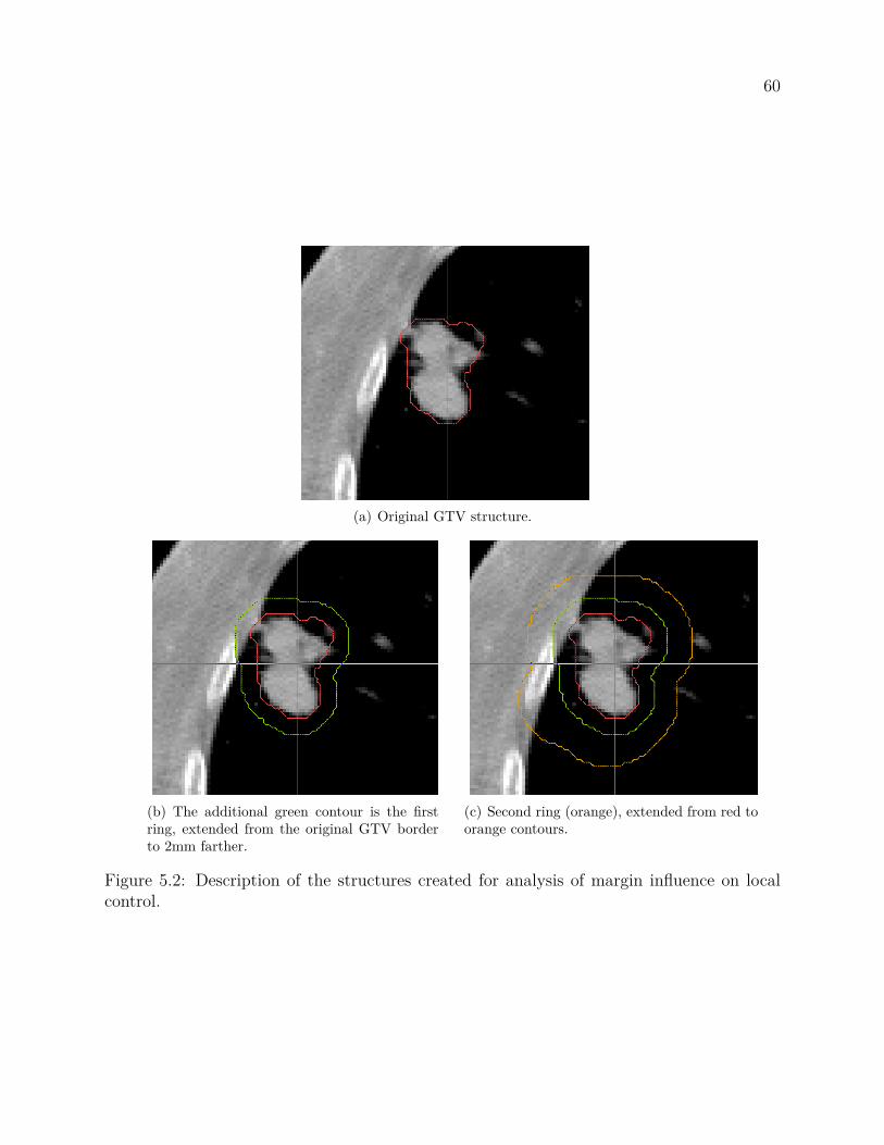
60

(a) Original GTV structure.

(b) The additional green contour is the firstring, extended from the original GTV borderto 2mm farther.

(c) Second ring (orange), extended from red toorange contours.

Figure 5.2: Description of the structures created for analysis of margin influence on localcontrol.

61

Therefore, isotropic random shifts (i.e. same range of variation on each direction)

were sampled from normal distributions with the same standard deviation (SD = 0.3 cm) for

the HN cohort. Anisotropic simulations were performed for the NSCLC dataset, giving it a

greater variability to the supero-inferior direction (SD = 0.6 cm), based on previous published

studies.66 On the other 2 directions the standard deviation was set to 0.3 cm.

Based on mean number of treatment fractions of each cohort, 35 daily shifts were

applied to the HN dataset and 30 to the NSCLC dataset to create the simulated dose

distributions. The simulated as well as the planned dose distributions were analyzed and

compared to each other in order to determine their influence on local control. Figure 5.1

shows an example of the simulated final DVH for the GTV in a NSCLC patient.

5.2.4 Data analysis

Patient data extraction and manipulation of a wide range of treatment plan characteristic

was made using CERR. This tool is built in MATLAB® (MathWorks, Natick, MA), which

was further utilized for data analysis.

Correlation with LC was quantified using the area under the receiver operating char-

acteristic curve (AUC) and Spearman’s rank correlation coe�cient (Rs) with its respective

p-value. These metrics were chosen because are suitable to correctly show the performance

of a binary classifier. The selection of these metrics has been discussed in detail in Section

3.2.2.2. The AUC is a measure of the classification accuracy. For perfect classification of the

observed versus the predicted results, AUC is 1. Random assignment of outcome results in

an AUC near 0.5.

These metrics were calculated for the planned (unshifted) and for the simulated

dose distributions to evaluate correlation of the originally contoured GTV (0 mm margin),

62

and the GTV plus each ring structure at a time (2 mm margin, and so forth). A logistic

regression model was built using the cEUD formula calculated for the margins and for the

GTV, i.e. a two variable logistic regression was evaluated.

Model validation and overfitting was assessed using bootstraps cross-validation

techniques. This technique consists of random partition of the dataset in two subsets, one

used for training and the other for testing the model. Bootstraps CV has been explain in

detail in Section 3.2.2.3.

5.3 Results

The correlation of LC with all margins (ring structures) cEUD values resulted statistically

significant (i.e. p-value < 0.05), even on CV, for both datasets.

For HN, the Spearman correlation ranks of LC and cEUD are summarized in Figure

5.3. The plots compare the planned dose distributions with the averaged (over the trials)

integral simulated dose distributions. We can observe that correlations follow the same

pattern on both dose distributions, although the margin e�ect is modulated and a bit less

correlated for the simulated DD.

A second finding is that there is an apparent increase in the predictive power at

10 mm margin when evaluating the model on the entire dataset, Figure 5.3(a). However,

when tested on CV (Figure 5.3b) all margins resulted less predictive than the model based

on the GTV alone i.e. 0 mm margin. On the CV scenario, they again follow more and less

the same pattern, except for the increase correlation at 10 mm on the planned DD.

It is also worth to point out that correlation of the planned dose distribution is

always stronger (higher Rs values) than for the simulated DD at all margin sizes. We can

63

(a) Results for the analysis of the margin influence on LC in HN

(b) Results for the analysis of the margin influence on LC in HN.

Figure 5.3: Results for the analysis of the margin influence on LC in HN.

64

(a) Results for the analysis of the margin influence on LC in NSCLC

(b) Results for the analysis of the margin influence on LC in NSCLC.

Figure 5.4: Results for the analysis of the margin influence on LC in NSCLC

65

hypothesize that adding a margin to a GTV for a HN treatment does not increase local

control since the immobilization devices and the positioning aids (such as IGRT) allows for

a good localization of the tumor, reflected in less misses, and also because the tumor does

not move within the HN region as it might happen in other sites.

Contrary to the HN case, for NSCLC we could say that correlations follow the

same shape on both DD only up to a margin of 5 mm. It is also not true in this case, that

correlation for the planned DD is always higher than for the simulated one. The correlation

results are plotted on Figure 5.4.

Figure 5.4(a) shows a correlation comparison between margins on the planned and

simulated DD. We can see an increase on the predictive power of the simulated DD for the

0 and 2 mm margins, a certain agreement but less strong at 5 and 10 mm, and then a rapid

fallo� at 15 mm, while the planned DD maintains correlation from 5 mm on.

When cross-validated, from 0 to 10 mm the simulated DD has higher predictive

power and both follow the same shape, as seen in Figure 5.4(b). After the 10 mm margin

point we again observe a rapid drop in predictive power for the simulated DD, phenomena

not seen on the planned DD.

We can observe an interesting valley at 2 mm of the cross-validated correlation

ranks (Figure 5.4b). This fallo� in power correlation indicates that adding a 2 mm margin

does not add predictive power to the model, but it does by adding a 5 mm one. It can

also be said that a 10 mm margin does not represent a gain on LC compared to the 5 mm

margin.

66

5.4 Discussion

Safety margins around the target volume are used in order to account for tumor position

uncertainties, minimizing the chances to miss the tumor. This study investigated the ef-

fect of using motion-inclusive dose distributions, obtained from a relatively simple motion

model, to eventually improve prediction of local control in HN and NSCLC cohorts while

not incrementing morbidity.

When delivered doses di�er from the treatment plan and change on a daily basis,

predictions of clinical outcome based on that original treatment plan become more uncertain.

Furthermore, predictions are based on the assumption that a constant dose per fraction is

actually delivered. The biological impact of unintentionally varying dose distributions over

the course of an entire treatment is a topic of current research and remains an unanswered

question.

The results of this study may indicate that fitting outcome data with shifted dose

distributions might be more accurate than fitting data to the planned dose distribution itself.

It has been also shown that a reduction in margin sizes for HN treatments is possible, and

that correlation with LC augmented when using the motion simulated DD. Although further

studies must be conducted in order to implement this reductions in clinical practice, if it

could be done, salivary glands will have higher chances to be spared and therefore patients

will be able to have a better quality of life.

Our analysis suggests that in HN the dose given to the tissue surrounding the GTV

is not correlated with LC, but it is for NSCLC. This may be because immobilization devices

and setup verification systems are more accurate in HN than in 3DCRT lung treatments,

added to the fact that the head and neck region is not as movable while thorax is. Even

67

though the cross-validated results indicate that the planned DD correlates better than the

simulated one, the need for margins up to 1 cm is very realistic.

Next Chapter will present testing results of the proposed LC predictive model. An

comprehensive analysis of the model’s external validation in a independent HN and NSCLC

datasets will be presented.

68

Chapter 6

External gTD model validation

6.1 Introduction

The purpose of the current chapter is to validate the new proposed gTD model for local

control prediction for patients that undergo radiotherapy treatment in head and neck and

non-small cell lung cancers. If the model can be validated, it could be used in clinical practice

to predict which patients are at risk of local recurrence given a certain treatment plan, prior

to delivery. This way, physicians would be able to change treatment parameters in order to

maximize the probability of LC.

Regression models are powerful tools frequently used in clinical settings to predict

the prognosis and/or the morbidity of a determined treatment. However, an important

problem is whether results of a model fitted or optimized on a certain cohort can be applied

to patients treated elsewhere.

Since each model is mathematically optimized to best fit the data on which it is

built, any analysis of prediction performance using the same dataset, or cross-validation

69

techniques on it (i.e. using random subsets of the same data), is biased towards the model.

Therefore, it is highly recommended that such a model would be validated on external

independent data, that is, data not used for the creation of the predictive model.

The main ways to assess or validate the performance of a prognostic model on a

new dataset are to compare agreement between predicted probabilities and observed out-

come rates (calibration), and to quantify the model’s ability to distinguish between patients

with and without the outcome been studied (discrimination). Calibration and discrimina-

tion are the main sources of deviation of individual predicted probabilities from the actual

outcomes.

A common measure of squared error is the chi-square goodness-of-fit statistic. The

goodness-of-fit allows for testing whether the observed proportions for a variable di�er from

estimations. Specifically to this work, model performance was tested using the Pearson

chi-square statistic since the study concerns a binary variable. Also, calibration and dis-

crimination analysis was performed independently.

6.2 Methods and material

6.2.1 Training cohort

The training cohorts were an HN and NSCLC cancer patient sets already described in

Chapter 3. In order to facilitate comprehension, a summary description will be stated

here.

The HN cohort consisted of 80 patients with SCC of the HN treated definitively

with IMRT, to a median dose of 70 Gy with standard fractionation of 2 Gy per fraction at

70

Washington University in Saint Louis. 23 patients presented primary tumor recurrence (local

failure). The median follow-up time was 19 months with a range of 2 to 137 months.

NSCLC cohort consisted of 56 patients treated with 3DCRT to prescription doses

ranging from 50 to 90 Gy, and standard fractionation (1.8-2.2 Gy/day) at Washington Uni-

versity in Saint Louis. From these, 22 patients failed locally (radiographic, or biopsy evidence

of progression was observed). Median follow-up time for all patients was 20 months, ranging

from 1 to 74 months. Dose distributions were Monte Carlo-corrected for the analysis.

6.2.2 Validation cohort

Head and Neck

All Memorial Sloan-Kettering Cancer Center (MSKCC) HN cancer patients with histologi-

cally confirmed oropharyngeal carcinoma (OPC) treated consecutively with definitive IMRT

and standard fractionation, between 1998 and 2009 were considered for inclusion. Definitive

treatment was defined as initiation of RT within 6 months of diagnosis. Two patients were

treated with RT more than 6 months after biopsy diagnosis and therefore were excluded.

Standard fractionation was defined as 2 Gy per fraction to a total of 70 Gy with simultaneous

integrated boost. Most patients received concurrent chemotherapy.

Among a total of 279 oropharynx patients with restorable treatment plans, all

patients with tonsil tumors were excluded (n=114). From the patients that were left, 113

plans that have the GTV-T contoured and retrievable plans were converted to CERR format

for analysis. From these patients only 6 had local recurrence.

Patients were evaluated weekly during RT. After the completion of radiation, pa-

tients were evaluated every 2-3 months for the first 2 years and every 4-6 months thereafter.

At each follow-up visit, a physical examination was performed, including flexible fiberoptic

71

endoscopy and palpation of the neck. A positron emission tomography scan as well as CT or

magnetic resonance imaging scan of the oropharynx and neck was performed approximately

3 months after treatment. Recurrences were all verified with biopsy.

NSCLC

For this validation cohort, medically inoperable consecutive patients with NSCLC treated

between 2001 and 2009 using 3DCRT, at Washington University in Saint Louis (WU) were

considered for analysis. The prescription doses ranged between 46 and 76 Gy. Concurrent

chemotherapy was administered to some patients, other received pre-treatment, or both.

Of these patients, only 116 patients had GTV-T contoured with restorable dose data and

entered to this analysis. 35 patients recurred at primary site. Median follow-up time for these

patients was 22 months, ranging from 2 to 122 months. There is no information available

at this time on how recurrence was evaluated, neither on followup evaluation. In both cases

the elapsed time to treatment failure was calculated using the first day of RT as the starting

point.

6.2.3 Proposed predictive model

A complete description of the gTD model proposed in this dissertation, its assessment and

parameter fitting process is given in detail in chapter 4. For completeness, the equation used

to compute gTD is the following:

gTD = ≠1– + Dref—

ln

C1

Vref

binsÿ

i=1Vi exp(≠–Di ≠ —DiDref )a

D1/a

. (6.1)

72

Table 6.1: Logistic regression parameters for HN and NSCLC LC gTD models, obtained inSection 4.3.3.

HN NSCLC

b0 0.14 0.09b1 -9.5 -5.9

The best fit parameter value was a = 0.3 for both data sets, using an – = 0.3 andÔ

— = 0.24. The logistic regression coe�cients for HN and NSCLC models summarized in

Table 6.1.

6.2.4 Performance measures

Goodness-of-fit

The goodness-of-fit of describes how well it fits a set of observations. Measures of goodness

of fit typically summarize the discrepancy between observed values and the values expected

under the model in question, i.e. a measure of the squared error.

The data studied here is of the categorical (dichotomous or binary) type, because

there is control or not. In this case, Pearson’s chi-squared test it is the most suitable to

analyze model performance. Pearson’s chi-squared test uses a measure of goodness-of-fit

which is the sum of di�erences between observed and expected outcome frequencies (that is,

counts of observations), each squared and divided by the expectation:

‰2 =Nÿ

i

(Oi ≠ Ei)2

Ei

, (6.2)

73

where: N is the number of bins, Oi is the observed frequency (count) and Ei is the expected

frequency (from the model) for bin i. The resulting value can be compared to the chi-squared

distribution to determine the goodness-of-fit.

It is noted that the model does not fit well the validation sample when ‰2 largely

exceeds the degrees of freedom. In order to determine the degrees of freedom of the chi-

squared distribution, one takes the total number of observed frequencies and subtracts the

number of estimated parameters. The test statistic follows, approximately, a chi-square

distribution with (k ≠ c) degrees of freedom where k is the number of non-empty bins and

c is the number of estimated parameters for the distribution.

Yet another way to check if the model fits well the validation set, is to look at

a probability plot of the Pearson residuals. When these are normalized and the model

fits reasonably to the data, they have roughly a standard normal distribution (without the

normalization, the residuals would have di�erent variances).

Calibration

Calibration refers to the agreement between observed outcomes and predictions, in other

words, to the accuracy of the model. A graphical assessment is the simplest and cleaner

way to study model calibration. The plot has predictions on the x-axis, and the outcome on

the y-axis. Perfect predictions should be on the 45° line. However, for the binary outcome

studied here, the plot contains only 0 and 1 values for the y-axis. There are smoothing

techniques that can be used to estimate the observed probabilities of the binary outcome

(p(y=1)) in relation to the predicted probabilities. In this work, results for subjects with

similar probabilities were plotted, and thus compared the mean predicted probability to the

mean observed outcome.

74

The calibration plot is characterized by an intercept, which indicates the extent

that predictions are systematically too low or too high, and a slope. At model building,

the intercept is equal to zero and the slope is 1 for regression models. At validation, slopes

smaller than 1 are common, and could be reflecting overfitting of a model.

Discrimination

Accurate predictions discriminate between those with and those without the outcome. Sev-

eral measures can be used to indicate how well we classify patients in a binary prediction

problem. For the analysis made here, the sensitivity and specificity were computed.

The sensitivity (also called the true positive rate) measures the proportion of actual

positives which are correctly identified as positives (for instance in this case, the percentage

of controlled patients who are correctly identified as having LC), mathematically:

sensitivity = True positive rateTrue positives + False negatives . (6.3)

The specificity (called the true negative rate) measures the proportion of negatives

which are correctly identified as such (e.g., the percentage of local failures that are correctly

identified as not having LC), it can be write as:

specificity = True negative rateTrue negatives + False positives . (6.4)

The perfect model, will be 100% sensitive and 100% specific, in other words dis-

crimination will be perfect. However, for any test, there is usually a trade-o� between these

measures. This trade-o� can be represented graphically as a receiver operating character-

75

istic (ROC) curve. The ROC curve plots the sensitivity against the false positive rate (1≠

Specificity).

6.3 Results

Model performance in the new HN cohort of 113 patients (6 with local failure) was almost

as good as at the building dataset for several reasons. First, the probability plot of the

Pearson’s chi squared residuals, Figure 6.1, shows a nice agreement of the residuals with a

normally distributed function. This indicates that the overall performance of the proposed

HN model is capable of describing the new dataset.

In contrast, Figure 6.2 for NSCLC model validation shows a huge discrepancy

between residuals and the normal distribution. This result forecast a bad model performance

for this cohort.

Second, the HN model was well calibrated. Figure 6.3 compares observed and

predicted event rates for the validation HN cohort based on the proposed gTD formulation.

The graph was obtained from dividing the patients into 11 bins with 11 patients each, except

the last one that had 13 patients in it. Fitting a linear trend to it, we obtained a slope very

close to 1 (0.999) and a intercept near zero (0.0012). This means that our gTD model

predictions in HN are not either systematically low or high, and that they keep the same

LC probability rate as the actual LC.

On the other hand, slope and intercept values of the NSCLC validation are poor.

Figure 6.4 shows a slope very far from the ideal 1 (0.21) and a intercept that cannot be

neglected (0.25). It can be observed that two bins (1 and 3) represent the higher disagree-

ments.

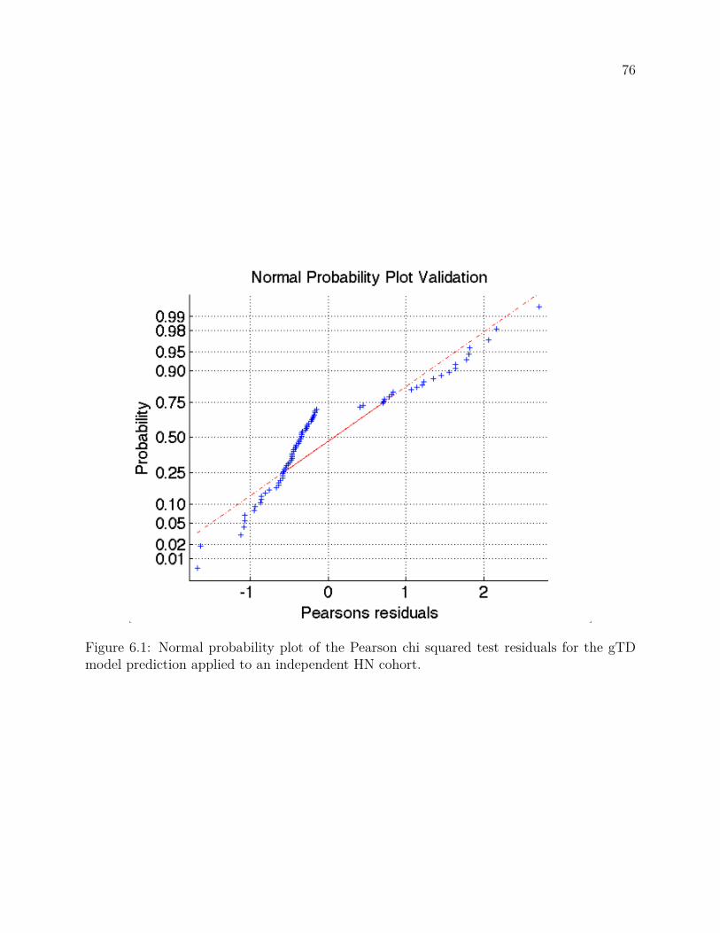
76

Figure 6.1: Normal probability plot of the Pearson chi squared test residuals for the gTDmodel prediction applied to an independent HN cohort.

77

Figure 6.2: Normal probability plot of the Pearson chi squared test residuals for the gTDmodel prediction applied to an independent NSCLC cohort.

78

Figure 6.3: Model calibration curve for prediction of LC in a 113 HN patients from MSKCC.The blue squares are the observed rates when patients are grouped into 11 bins (the last bincontaining 13 patients, and all other with 11 each), with their respective error bars. The redline represents the linear trend of the data, described by the equation also in red.

79

Figure 6.4: Model calibration curve for prediction of LC in a 116 NSCLC patients from WU.The blue squares are the observed rates when patients are grouped into 11 bins (the last bincontaining 16 patients, and all other with 11 each), with their respective error bars. The redline represents the linear trend of the data, described by the equation also in red.

80

Figure 6.5: ROC plot for HN model validation. In this case AUC = 0.807, where AUC = 1represents the perfect model.

The third performance evaluation test was discrimination. According to Figure

6.5, which shows the ROC plot of the HN prediction results, the proposed model retained

discrimination in the new HN cohort. Moreover, the AUC value was very high (0.807) which

leads to get very optimistic about this model. However, the recurrences in this cohort were

very few (6 patients, about 5%) and this might be the primary reason for such a high AUC.

Therefore, a closer look by examining the box plot for this cohort is needed.

Figure 6.6 is a box plot of the predicted probabilities of LC in the validation

dataset. The edges of the box are the 25th and 75th percentiles, the whiskers extend to

the most extreme data points not considered outliers, and outliers are plotted individually

(red crosses). Points are drawn as outliers if they are larger than q3 + w(q3 ≠ q1) or smaller

81

Figure 6.6: the central mark is the median, the edges of the box are the 25th and 75thpercentiles, the whiskers extend to the most extreme data points not considered outliers,and outliers are plotted individually.

than q1 ≠ w(q3 ≠ q1), where q1 and q3 are the 25th and 75th percentiles, respectively, and w

is the whisker length.

We can see that, even though the groups (controls and failures) are mainly over-

lapped, the median values are very distinctive. It is also noticeable the long bottom whisker

for the control group, many patients who are ranked with low gTD values were controlled

as well. This may be due to the fact that in the New York City area the incidence of HPV

positive HN cancers (more sensitive to radiation) patients is higher than in the Midwest

(where the building cohort is from).

82

Figure 6.7: ROC plot for NSCLC model validation. AUC = 0.5 means that the model doesnot perform better than random guess, and an AUC of 1 reflects the perfect model.In thiscase AUC = 0.535

Discriminations results for NSCLC model predictions, illustrated in Figure 6.7,

corroborated the results obtained by the Pearson’s residuals analysis. AUC value was 0.535

which indicates that in this case, the model performs very poorly, close to the performance

of random assignment.

The complete analysis can be summarized in the logistic regression model plot,

Figure 6.8 for HN and 6.9 for NSCLC. For HN, white circles represent failures (barely seen,

only 6), blue squares symbolize the observed control rate at each of the 11 bins the data was

divided into, with their respective error bars and the bin control rate. It is evident that we

are looking at the upper "shoulder" of this supposed "S" shaped prediction curve, due to the

high overall control rate (107/113, 95%). Despite that, all data points are well fitted to this

83

Figure 6.8: Dose response curve computed from the proposed predictive model applied toan external HN validation set.

curve, which confirms that this independent external HN cohort is well represented by the

model proposed in this dissertation.

For completeness, the logistic regression NSCLC model curve is also included (Fig-

ure 6.9). We can observe a wide variation in gTD values, ranging from approximately 12 to

88 Gy, in contrast to the range obtained for HN (5̃0-80 Gy). We can also see that the 3 first

data points (control rate at bin) fall outside the 95% CI. If we only look at the other data

points, we could say that the model performs well.

The poor results in the NSCLC model validation were confirmed by refitting the

model on the data of the validation set. In this case the AUC was also close to 0.5 and not

statistically significant (p>0.5), for all possible values of the exponent a.

84

Figure 6.9: Dose response curve computed from the proposed predictive model applied toan external NSCLC validation set.

85

6.4 Discussion

Biologically based correlation models for plan optimization and/or evaluation have been

introduced for clinical use. There is an inclination towards the use of these models because

they would reflect clinical RT goals better. However, biologically based treatment planning

is not being widely used in clinical practice due to the lack of validation and impact studies,

which is currently an active area of research.

The work presented in this Chapter is a validation of the model that this dissertation

proposes. The idea of finding a relatively simple model, that could be used transversely

through tumor types and patient populations is very attractive, yet highly unlikely. It is

well known that tumors respond di�erently to RT (e.g., lymphomas and sarcomas), and even

within the same type of tumor there are clinical factors that can modify their response to

RT (such as HPV in HN).

Accordingly, the findings made studying the validation of the gTD model reflects

that fact. After applying the model built on a HN dataset from WUSTL to a HN cohort

collected at MSKCC in New York, we found: (a) a almost perfect model calibration (cali-

bration curve slope = 0.999, and intercept = 0.0012); and (b) a reasonable discrimination

between controls and failures, in spite of the few recurrences (n = 6/113, 5%). In summary,

a good model performance on an external dataset. However, the NSCLC model could not

be validated in a cohort from the same institution (WUSTL).

The poor performance on cohorts of the same institution can be explained by the

same reasons why do not work for di�erent ones. Firstly, it could be that the patients

from di�erent cohorts belong to di�erent attending physicians, which was the case. Another

reason could be that our model building dataset had DD calculated using Monte Carlo,55

and the validation set was not. Yet another thing to look at is the small number of patients

86

used to build the model (n = 56). A model built on a small dataset might limit the model

applicability.

All those things are necessary to bear in mind when using a predictive model. It is

necessary to emphasize that a model can only be applied safely to other groups of patients if

these groups are comparable to the study population, in terms of clinical as well as treatment

characteristics. For instance, it is not advisable to apply our model to patients treated with

stereotactic radiosurgery since it was built considering standard fractionation schemes.

The results presented in this Chapter suggest that the gTD formulation has poten-

tial to be used for biologically based treatment planning in HN treatments. However, before

setting the model into routine clinical practice, it must be validated with institutional ret-

rospective data to make sure it performs well with your patient characteristics.

87

Chapter 7

Conclusions and future directions

7.1 Conclusions

The main purpose of this dissertation was to find ways to improve local control in head and

neck and non-smal cell lung cancer patients, by means of a retrospective outcome analy-

sis.

First, a comprehensive study correlating all clinical and dosimetric parameters with

LC was made. According to the literature,20–23 the results showed that tumor volume is

among the best LC predictors. It was also found that the gEUD formula, though it has been

demonstrated that correlates well with toxicity,39 is not useful to rank treatment plans in

terms of LC on HNSCC and NSCLC tumors (Figure 3.6).

On the other hand, the volume-corrected cEUD formula28 is the available parameter

that correlates best with LC. However, the better correlations were obtained fitting relatively

high values of the radiosensitivity parameter –. – has been extensively studied in in vitro

and in vivo assays.60 The widely accepted values do not correspond to the best fit (SF2 =

88

0.8 for both datasets). Hence, this dissertation sought a model that could reflect known

radiobiological values. The first attempt to do so, was to introduce an "e�ective" SF2 value

which varied with tumor sizes. This approach, although correlated as well as the cEUD

for reasonable – values, did not improve the model since it kept selecting high values when

optimized for the best correlation.

In Chapter 4 a new proposed EUD formulation was introduced, the gTD, which

showed high LC correlations bridging the gap between correlation and already known ra-

diobiological parameters. This model depends on the exponent (a) which is translated as a

weighing parameter of hot or cold spots in the tumor. The best-fit a (ranging from 0.2 to

0.3) was substantially less than 1.0, indicating that high-dose regions are more important for

local control than implied by the independent cell kill formulas normally used to estimate

tumor control.

While cEUD is highly dependent on SF2 as seen in Figure 3.6, gTD seems insen-

sitive to the radiosensitivy parameter – in these two cohorts (Figure 4.3). This is because

gTD is a sort of generalized mean of the surviving fractions.

Then, our gTD model was validated in independent cohorts (one HN and one

NSCLC), obtaining contradictory results. For HN, the model predicts reasonably well

at other institution, and in the NSCLC case the prediction is not statistically significant

(p>0.05). This may be attributed to the poor dose calculation for 3DCRT treatments

(without convolution superposition algorithms), since the NSCLC model was built on a

Monte-Carlo corrected dose distribution.55 The small number of patients on the model

building dataset (n=56) may also limit its use on other patient sets. Nonetheless, a step

forward could be taken with the gTD model for HN.

This dissertation also examined margins influence on LC (Chapter 5). In order to

do this, di�erent random positioning errors were simulated for each treatment fraction for

89

both datasets. Then each of these delivered DD were integrated to analyze the LC correlation

with the dose given to di�erent margin sizes. The higher correlation coe�cients obtained

implies that motion simulated DD correlates LC more accurately. The results also suggest

that a reduction in margin sizes for HN might be possible, since predictive power did not

increase with larger margins as compared to the 0 margin (GTV only) on cross-validation.

Unlike the HN case, in NSCLC margins up to 10 mm increased the correlation with LC.

However, in order to translate these findings to clinical practice, external validation and then

prospective studies must be carried out.

In summary, with further testing and caveats, a margin revision could be imple-

mented in clinical practice. Also, with the same care taken, the well-studied DVH constraint

known to work could be complemented with the gTD model proposed in this disserta-

tion.

7.2 Future directions

The gTD parameter was originally formulated as the dose that would lead to the same

overall expected cell survival for a reference dose per fraction of 2 Gy, taking into account

total dose and neglecting fraction size and OTT. In order to apply the gTD formulation

to treatments using di�erent dose fractionation schemes, gTD should include a correction

factor that accounts for dose per fraction, number of fractions and OTT. This correction

factor could be based on the biologically e�ective dose (BED).

Another aspect to be further studied is the use of motion simulated DD on predic-

tion models. As shown in Chapter 5, LC is more accurately correlated when using motion

simulated dose distributions. It is not practical to obtain motion simulated DD for all treat-

90

ment plans you need to compare or evaluate. However, it is necessary to study whether a

model built on motion simulated dose distributions will be more accurate.

The topic of this dissertation is an active area of research, and there are several

issues that need to be studied. An important question still unanswered is at what point a

rule has been su�ciently validated and updated. Future research should address the question

of how many validation studies and what type of adjustments are needed before it is justified

to implement a prediction model into clinical practice.

Further, the performance of a prediction model may worsen over time, as it may

become outdated. It is worthwhile to evaluate periodically whether the accuracy of the

prediction holds over time. And, of course, the question of how often these revisions should

be made is open and needs to be addressed.

91

Appendix A

Implementation of gTD function in

MatLab®

The gTD formula was implemented as a function in Matlab® using the following (.m)

code:

function [Rss, ind, ps, AUCm, a] = getEUD(database, dvhName, option, alpha)

%% cEUD-based logistic TCP model

EUD = [];

SF2=exp(-2*alpha - 4*(0.241)^2);

Vref = 14; OTTref = 42; Dref=2;

expo = [-10:.1:-.1 .1:.1:10]; %WashU; HN%[-23:.1:-.1 .1:.1:19.8];

T_k = 21; T_p = 5;

outcome = [ddbs.outcome]’;

if(~isfield(ddbs, dvhName))

92

error([’specified DVH ’ dvhName ’ is not a field’]);

else

for j=1:length(expo)

for i = 1:length(ddbs)

doseV = []; volumeV = [];

doseV = ddbs(i).(dvhName)(1,:);

volumeV = ddbs(i).(dvhName)(2,:);

Vtot(i) = sum(volumeV);

switch lower(option)

case ’prolif’ % proliferation effect

EUDM(i,j)= Dref*log(2.^((Ttime(i)-T_k)./T_p).*sum(volumeV.* SF2(j).^ ...

... (doseV./Dref))./10 ./(2.^((OTTref-T_k).T_p)))/log(SF2(j));

case ’gTD’

EUDM(i,j)= Dref*log((sum(volumeV.* ((SF2.^(doseV./Dref)).^ ...

... expo(j))./Vref)).^(1/expo(j)))/log(SF2);

case ’gEUD’

EUDM(i,j)= (sum((volumeV./Vtot(i)).* (doseV.^(expo(j))))).^(1/expo(j));

case ’gv’ % generalized with Veffect

EUDM(i,j)= (sum(volumeV.* (doseV.^(expo(j))))./Vref).^(1/expo(j));

end

end

[b, ~, stats] = glmfit(EUDM(:,j), outcome,’binomial’);

mu = glmval(b, EUDM(:,j),’logit’,stats);

[Rss(j) ps(j)] = corr(mu, outcome, ’type’, ’spearman’);

[~,~, ~,AUCm(j)] = perfcurve(outcome,mu,1);

93

end

[maxRs, ind] = max(Rss);

a = expo(ind);

end

The following code was used for the bootstrap CV.

%% Bootstrap CV

niter = 3000;

NPat = length(data);

B = [];

%<NPat x niter> matrix w/ rand-Sampled sets

sample = drxlr_pseudo_sample(NPat,NPat,niter);

for iter=1: niter

dataTrain = data(sample(:,iter),:);

outcTrain = outcome(sample(:,iter));

indtest = setdiff([1:NPat]’,sample(:,iter));

dataTest = data(indtest,:);

outcTest = outcome(indtest);

[muTrain, b, pval] = drxlr_apply_logistic_regression(dataTrain,outcTrain);

muTest = drxlr_logit_fun(dataTest, b);

[rs(iter), ps(iter)] = spearman(muTest,outcTest);

B = [B b];

94

end

b0 = B(end,:);

b1 = B(1,:);

figure ;

subplot(2,2,1,’fontSize’,14)

hist(b0, 100);

title(’b0 histogram’,’fontsize’,14)

subplot(2,2,2,’fontsize’,14)

hist(b1, 100);

title(’b1’,’fontsize’,14)

subplot(2,2,3,’fontsize’,14)

hist(rs, 100);

title(’Rs’,’fontsize’,14)

subplot(2,2,4,’fontsize’,14)

hist(ps, 100);

title(’p value’,’fontsize’,14)

BMean = mean(B’) %b1Mode = mode(b1)

std(b0);

std(b1);

rsMean = mean(rs)

std(rs);

pMean = mean(ps)

std(ps);

pGmean = geomean(ps)

95

Bibliography

[1] Carlos A. Perez. Principles and practice of radiation oncology. Lippincott Williams &

Wilkins, Philadelphia, 4th edition, 2004.

[2] W. M. Mendenhall, C. G. Morris, R. J. Amdur, R. W. Hinerman, and A. A. Mancuso.

Parameters that predict local control after definitive radiotherapy for squamous cell

carcinoma of the head and neck. Head and Neck-Journal for the Sciences and Specialties

of the Head and Neck, 25(7):535–542, 2003.

[3] M. K. Martel. Advanced radiation treatment planning and delivery approaches for

treatment of lung cancer. Hematology-Oncology Clinics of North America, 18(1):231–

+, 2004.

[4] Gunilla C. Bentel. Radiation Therapy Planning. McGraw-Hill Professional, 2nd edition,

1996.

[5] H. D. Suit and S. J. Westgate. Impact of improved local control on survival. Interna-

tional Journal of Radiation Oncology Biology Physics, 12:453–458, 1986.

[6] Rodney R. Million and Nicholas J. Cassisi. Management of head and neck cancer : a

multidisciplinary approach. Lippincott, Philadelphia, 2nd edition, 1994.

[7] S. Clavel, M. P. Charron, M. Bélair, G. Delouya, B. Fortin, P. Després, D. Soulières,

E. Filion, L. Guertin, and P. F. Nguyen-Tan. The role of computed tomography in

96

the management of the neck after chemoradiotherapy in patients with head-and-neck

cancer. Int J Radiat Oncol Biol Phys, 2011.

[8] V. A. Passero, B. F. Branstetter, Y. Shuai, D. E. Heron, M. K. Gibson, S. Y. Lai, S. W.

Kim, J. R. Grandis, R. L. Ferris, J. T. Johnson, and A. Argiris. Response assessment by

combined pet-ct scan versus ct scan alone using recist in patients with locally advanced

head and neck cancer treated with chemoradiotherapy. Ann Oncol, 21(11):2278–83,

2010.

[9] J. Bourhis, J. Overgaard, H. Audry, K. K. Ang, M. Saunders, J. Bernier, J. C. Horiot,

A. Le Maître, T. F. Pajak, M. G. Poulsen, B. O’Sullivan, W. Dobrowsky, A. Hliniak,

K. Skladowski, J. H. Hay, L. H. Pinto, C. Fallai, K. K. Fu, R. Sylvester, J. P. Pignon,

Meta-Analysis of Radiotherapy in Carcinomas of Head, and neck (MARCH) Collabo-

rative Group. Hyperfractionated or accelerated radiotherapy in head and neck cancer:

a meta-analysis. Lancet, 368(9538):843–54, 2006.

[10] A. A. Mancuso, S. K. Mukherji, I. Schmalfuss, W. Mendenhall, J. Parsons, F. Pameijer,

R. Hermans, and P. Kubilis. Preradiotherapy computed tomography as a predictor of

local control in supraglottic carcinoma. J Clin Oncol, 17(2):631–7, 1999.

[11] Eric J. Hall and Amato J. Giaccia. Radiobiology for the radiologist. Lippincott Williams

& Wilkins, Philadelphia, 6th edition, 2006.

[12] D. M. Brizel, R. K. Dodge, R. W. Clough, and M. W. Dewhirst. Oxygenation of

head and neck cancer: changes during radiotherapy and impact on treatment outcome.

Radiotherapy and Oncology, 53(2):113–117, 1999.

[13] S. Damast, S. Wolden, and N. Lee. Marginal recurrences after selective targeting with

intensity-modulated radiotherapy for oral tongue cancer. Head Neck, 2011.

97

[14] J.R Molina, P. Yang, S.D. Cassivi, S.E. Schild, and A.A. Adjei. Non-small cell lung can-

cer: epidemiology, risk factors, treatment, and survivorship. Mayo Clin Proc, 83(5):584–

594, 2008.

[15] D.E. Dosoretz, M.J. Katin, P.H. Blitzer, J.H. Rubenstein, S. Salenius, M. Rashid, R.A.

Dosani, G. Mestas, A.D. Siegel, and T.T. et al. Chadha. Radiation therapy in the

management of medically inoperable carcinoma of the lung: results and implications

for future treatment strategies. International Journal of Radiation Oncology Biology

Physics, 24(1):3–9, 1992.

[16] R. Arriagada. Current strategies for radiation therapy in non-small cell lung cancer.

Chest, 112(4):S209–S213, 1997.

[17] J. M. Watkins, A. E. Wahlquist, A. J. Zauls, E. C. Fields, E. Garrett-Mayer, E. G.

Aguero, G. A. Silvestri, and A. K. Sharma. High-dose fractionated radiotherapy to 80

gy for stage i-ii medically inoperable non-small-cell lung cancer. Journal of Medical

Imaging and Radiation Oncology, 54(6):554–561, 2010.

[18] R. Arriagada, T. Lechevalier, E. Quoix, P. Ru�e, H. Decremoux, J. Y. Douillard,

M. Tarayre, J. P. Pignon, and A. Laplanche. E�ect of chemotherapy on locally advanced

non-small-cell lung-carcinoma - a randomized study of 353 patients. International Jour-

nal of Radiation Oncology Biology Physics, 20(6):1183–1190, 1991.

[19] E. R. Velazquez, H. J. Aerts, C. Oberije, D. De Ruysscher, and P. Lambin. Prediction of

residual metabolic activity after treatment in nsclc patients. Acta Oncol, 49(7):1033–9,

2010.

[20] D. J. Brenner. Dose, volume, and tumor-control predictions in radiotherapy. Interna-

tional Journal of Radiation Oncology Biology Physics, 26(1):171–179, 1993.

98

[21] H. H. Dubben, H. D. Thames, and H. P. Beck-Bornholdt. Tumor volume: a basic and

specific response predictor in radiotherapy. Radiotherapy and Oncology, 47(2):167–174,

1998.

[22] J. Willner, K. Baier, L. Pfreundner, and M. Flentje. Tumor volume and local control in

primary radiotherapy of nasopharyngeal carcinoma. Acta Oncologica, 38(8):1025–1030,

1999.

[23] J. Willner, K. Baier, E. Caragiani, A. Tschammler, and M. Flentje. Dose, volume,

and tumor control predictions in primary radiotherapy of non-small-cell lung cancer.

International Journal of Radiation Oncology Biology Physics, 52(2):382–389, 2002.

[24] D. E. Lea. Action of Radiations on Living Cells. Cambridge: The University Press,

2nd edition, 1962.

[25] A.M. Kellerer and H. Rossi. The theory of dual radiation action. Top Radiat Res Q,

8:85–158, 1972.

[26] R.G. Dale. The application of the linear-quadratic dose-e�ect equation to fractionated

and protracted radiotherapy. British Journal of Radiology, 58:515–528, 1985.

[27] J.F. Fowler. The linear-quadratic formula and progress in fractionated radiotherapy.

British Journal of Radiology, 62:679–694, 1989.

[28] Andrzej Niemierko. Reporting and analizing dose distributions: a concept of equivalent

uniform dose. Medical Physics, 34(7):103–110, 1997.

[29] K. K. Fu, T. F. Pajak, A. Trotti, C. U. Jones, S. A. Spencer, T. L. Phillips, A. S. Garden,

J. A. Ridge, J. S. Cooper, K. K. Ang, and Grp Radiation Therapy Oncology. A radiation

therapy oncology group (rtog) phase iii randomized study to compare hyperfractionation

and two variants of accelerated fractionation to standard fractionation radiotherapy for

99

head and neck squamous cell carcinomas: First report of rtog 9003. International

Journal of Radiation Oncology Biology Physics, 48(1):7–16, 2000.

[30] J. C. Horiot, P. Bontemps, W. vandenBogaert, R. LeFur, D. vandenWeijngaert,

M. Bolla, J. Bernier, A. Lusinchi, M. Stuschke, J. LopezTorrecilla, A. C. Begg, M. Pier-

art, and L. Collette. Accelerated fractionation (af) compared to conventional frac-

tionation (cf) improves loco-regional control in the radiotherapy of advanced head and

neck cancers: results of the eortc 22851 randomized trial. Radiotherapy and Oncology,

44(2):111–121, 1997.

[31] W. Sause, P. Kolesar, S. Taylor, D. Johnson, R. Livingston, R. Komaki, B. Emami,

W. Curran, R. Byhardt, A. R. Dar, and A. Turrisi. Final results of phase iii trial in

regionally advanced unresectable non-small cell lung cancer - radiation therapy oncol-

ogy group, eastern cooperative oncology group, and southwest oncology group. Chest,

117(2):358–364, 2000.

[32] M. Saunders, S. Dische, A. Barrett, A. Harvey, D. Gibson, and M. Parmar. Continuous

hyperfractionated accelerated radiotherapy (chart) versus conventional radiotherapy in

non-small-cell lung cancer: A randomised multicentre trial. Lancet, 350(9072):161–165,

1997.

[33] Andrzej Niemierko. A generalized concept of equivalent uniform dose. Medical Physics,

26:1101, 1999.

[34] Q. W. Wu, D. Djajaputra, Y. Wu, J. N. Zhou, H. H. Liu, and R. Mohan. Intensity-

modulated radiotherapy optimization with geud-guided dose-volume objectives. Physics

in Medicine and Biology, 48(3):279–291, 2003.

[35] S. Webb, P. M. Evans, W. Swindell, and J. O. Deasy. A proof that uniform dose

gives the greatest tcp for fixed integral dose in the planning target volume. Physics in

100

Medicine and Biology, 39(11):2091–2098, 1994.

[36] N. Ploquin, I. Kay, A. Rangel-Baltazar, H. Lau, and P. Dunscombe. A comparison of

techniques for simulating set-up error and uncertainty in head and neck imrt. Medical

Physics, 33(9):3213–3219, 2006.

[37] A. L. Ho�mann, D. den Hertog, A. Y. D. Siem, Jham Kaanders, and H. Huizenga.

Convex reformulation of biologically-based multi-criteria intensity-modulated radiation

therapy optimization including fractionation e�ects. Physics in Medicine and Biology,

53(22):6345–6362, 2008.

[38] B. Choi and J. Deasy. The generalized equivalent uniform dose function as a basis for

intensity-modulated treatment planning. Physics in Medicine and Biology, 47(20):3579–

3589, 2002.

[39] K. L. Foweraker, K. E. Burton, S. E. Maynard, R. Jena, S. J. Je�eries, R. J. C. Laing,

N. G. Burnet, and neurosurgery Skull base surg. High-dose radiotherapy in the man-

agement of chordoma chondrosarcoma of the skull base and cervical spine: Part 1 -

clinical outcomes. Clinical Oncology, 19(7):509–516, 2007.

[40] T. S. Hong, W. A. Tome, R. J. Chappell, P. Chinnaiyan, M. P. Mehta, and P. M. Harari.

The impact of daily setup variations on head-and-neck intensity-modulated radiation

therapy. International Journal of Radiation Oncology Biology Physics, 61(3):779–788,

2005.

[41] Y. Kim and W. A. Tome. Dose-painting imrt optimization using biological parameters.

Acta Oncologica, 49(8):1374–1384, 2010.

[42] N. P. Orton and W. A. Tome. The impact of daily shifts on prostate imrt dose distri-

butions. Medical Physics, 31(10):2845–2848, 2004.

101

[43] S. Levegrun, A. Jackson, M. J. Zelefsky, E. S. Venkatraman, M. W. Skwarchuk,

W. Schlegel, Z. Fuks, S. A. Leibel, and C. C. Ling. Analysis of biopsy outcome after

three-dimensional conformal radiation therapy of prostate cancer using dose-distribution

variables and tumor control probability models. International Journal of Radiation On-

cology Biology Physics, 47(5):1245–1260, 2000.

[44] A. Terahara, A. Niemierko, M. Goitein, D. Finkelstein, E. Hug, N. Liebsch, D. O’Farrell,

S. Lyons, and J. Munzenrider. Analysis of the relationship between tumor dose inhomo-

geneity and local control in patients with skull base chordoma. International Journal

of Radiation Oncology Biology Physics, 45(2):351–358, 1999.

[45] R. McCammon, T. E. Schefter, L. E. Gaspar, R. Zaemisch, D. Gravdahl, and B. Ka-

vanagh. Observation of a dose-control relationship for lung and liver tumors after

stereotactic body radiation therapy. International Journal of Radiation Oncology Biol-

ogy Physics, 73(1):112–118, 2009.

[46] M. van Herk. Errors and margins in radiotherapy. Seminars in Radiation Oncology,

14(1):52–64, 2004.

[47] ICRU Report 50. Prescribing, Recording and Reporting Photon Beam Therapy. Inter-

national Commission on Radiation Units and Measurements, Bethesda, MD, 1993.

[48] ICRU Report 62. Prescribing, Recording and Reporting Photon Beam Therapy (Sup-

plement to ICRU Report 50). International Commission on Radiation Units and Mea-

surements, Bethesda, MD, 1999.

[49] C. W. Hurkmans, P. Remeijer, J. V. Lebesque, and B. J. Mijnheer. Set-up verification

using portal imaging; review of current clinical practice. Radiotherapy and Oncology,

58(2):105–120, 2001.

102

[50] L. K. Schubert, D. C. Westerly, W. A. Tome, M. P. Mehta, E. T. Soisson, T. R. Mackie,

M. A. Ritter, D. Khuntia, P. M. Harari, and B. R. Paliwal. A comprehensive assessment

by tumor site of patient setup using daily mvct imaging from more than 3,800 helical

tomotherapy treatments. International Journal of Radiation Oncology Biology Physics,

73(4):1260–1269, 2009.

[51] Y. Seppenwoolde, H. Shirato, K. Kitamura, S. Shimizu, M. van Herk, and J.V. Lebesque.

Precise and realtime measurement of 3d tumor motion in lung due to breathing and

heartbeat, measured during radiotherapy. International Journal of Radiation Oncology

Biology Physics, 53(4):822–834, 2002.

[52] K.E. Sixel, M. Ruschin, R. Tirona, and P.C. Cheung. Digital fluoroscopy to quantify

lung tumor motion: potential for patient-specific planning target volumes. International

Journal of Radiation Oncology Biology Physics, 57(3):717–723, 2003.

[53] P.J. Keall, G.S. Mageras, J.M. Balter, R.S. Emery, K.M. Forster, S.B. Jiang, and et al.

The management of respiratory motion in radiation oncology report of aapm task group

76. Medical Physics, 33(10):3874–3900, 2006.

[54] AAPM Task Group 166. The Use and QA of Biologically Related Models for Treatment

Planning. American Association of Physicists in Medicine, 2012.

[55] P. E. Lindsay, I. El Naqa, A. J. Hope, M. Vicic, J. Cui, J. D. Bradley, and J. O.

Deasy. Retrospective monte carlo dose calculations with limited beam weight informa-

tion. Medical Physics, 34(1):334–346, 2007.

[56] J. O. Deasy, A. I. Blanco, and V. H. Clark. Cerr: A computational environment for

radiotherapy research. Medical Physics, 30(5):979–985, 2003.

[57] P. Sprent and N.C. Smeeton. Applied nonparametric statistical methods. Boca Raton:

Chapman & Hall/CRC, 3rd edition, 2001.

103

[58] E. L. Kaplan and P. Meier. Nonparametric estimations from incomplete observations.

Am J Statist Assoc, 53:457–481, 1958.

[59] G.H. Fletcher. Textbook of Radiotherapy. Lea and Febiger, Philadelphia, 3rd edition,

1980.

[60] J.D. Chapman. Can the two mechanisms of tumor cell killing by radiation be exploited

for therapeutic gain? Journal of Radiation Research, 55:2–9, 2014.

[61] M. A. Deveau, A. N. Gutierrez, T. R. Mackie, W. A. Tome, and L. J. Forrest. Dosimetric

impact of daily setup variations during treatment of canine nasal tumors using intensity-

modulated radiation therapy. Veterinary Radiology & Ultrasound, 51(1):90–96, 2010.

[62] M. A. Hunt, G. J. Kutcher, C. Burman, D. Fass, L. Harrison, S. Leibel, and Z. Fuks.

The e�ect of setup uncertainties on the treatment of nasopharynx cancer. International

Journal of Radiation Oncology Biology Physics, 27(2):437–447, 1993.

[63] S. C. Erridge, Y. Seppenwoolde, S. H. Muller, M. van Herk, K. De Jaeger, J. S. A.

Belderbos, L. J. Boersma, and J. V. Lebesque. Portal imaging to assess set-up errors,

tumor motion and tumor shrinkage during conformal radiotherapy of non-small cell

lung cancer. Radiotherapy and Oncology, 66(1):75–85, 2003.

[64] H. C. J. de Boer, J. R. V. De Koste, S. Senan, A. G. Visser, and B. J. M. Heijmen.

Analysis and reduction of 3d systematic and random setup errors during the simulation

and treatment of lung cancer patients with ct-based external beam radiotherapy dose

planning. International Journal of Radiation Oncology Biology Physics, 49(3):857–868,

2001.

[65] J. Wang, R. M. Zhong, S. Bai, Y. Lu, Q. F. Xu, X. J. Zhou, and F. Xu. Evaluation of

positioning accuracy of four di�erent immobilizations using cone-beam ct in radiother-

104

apy of non-small-cell lung cancer. International Journal of Radiation Oncology Biology

Physics, 77(4):1274–1281, 2010.

[66] Hyejoo Kang, Ellen D. Yorke, Jie Yang, Chen-Shou Chui, Kenneth E. Rosenzweig, and

Howard I. Amols. Evaluation of tumor motion e�ects on dose distribution for hypofrac-

tionated intensity-modulated radiotherapy of non-small-cell lung cancer. JOURN AL

OF APPLIED CLINICAL MEDICAL PHYSICS, 11(3):78–89, 2010.