Generalized Sensitivity Analysis and

Application to Quasi-experiments∗

Masataka Harada

New York University

masatakaharada@nyu.edu

August 27, 2013

Abstract

The generalized sensitivity analysis (GSA) is a sensitivity analysis for unobserved

confounders characterized by a computational approach with dual sensitivity parame-

ters. Specifically, GSA generates an unobserved confounder from the residuals in the

outcome and treatment models, and random noise to estimate the confounding effects.

GSA can deal with various link functions and identify necessary confounding effects

with respect to test-statistics while minimizing the changes to researchers’ original es-

timation models. This paper first provides a brief introduction of GSA comparing its

relative strength and weakness. Then, its versatility and simplicity of use are demon-

strated through its applications to the studies that use quasi-experimental methods,

namely fixed effects, propensity score matching, and instrumental variable. These ap-

plications provide new insights as to whether and how our statistical inference gains

robustness to unobserved confounding by using quasi-experimental methods.

∗I thank Christopher Berry, Jennifer Hill, Luke Keele, Robert LaLonde, Andrew Martin, Marc Scott,Teppei Yamamoto for helpful comments on earlier drafts of this paper.

1 Introduction

Political science research nowadays commands a wide variety of quasi-experimental tech-

niques intended to help identify causal effects.1 Researchers often begin with collecting

extensive panel data to control for unit heterogeneities with difference in differences or fixed

effects. When panel data are not available or the key explanatory variable has no within-

unit variation, researchers typically match treated units with control units from a multitude

of matching techniques. Perhaps, they are fortunate to find a good instrumental variable

which is effectively randomly assigned and affects the outcome only through the treatment

variable. Researchers who use these techniques are tempted to report the results causally.

Of course, none of these methods ensures that the findings are causal. In contrast to

randomized experiments (assuming randomization is pristine), which randomize treatment

assignments in terms of both observed and unobserved confounders, these quasi-experiments

all rely on untestable assumptions (Heckman, Ichimura and Todd 1998; Smith and Todd

2005). In order to infer causality, researchers need to assume some version of ignorability

(Rubin 1978), also known as conditional independence or the absence of omitted variables,

and defend its validity to the readers. Although political scientists acknowledge that the

assumption of ignorability is “a strong condition” (Ho et al., 2007), few studies in the

discipline rigorously test this assumption as “it is one about which social scientists are

deeply knowledgeable” (Ho et al., 2007).2

However, the cost of blind acceptance of ignorability is nontrivial. LaLonde’s (1986)

pioneering work shows that the treatment effects estimated with observational data are

strikingly different from those of the randomized experiment, no matter what econometric

techniques are used.3 Thus, if researchers’ initial motivation to perform quasi-experimental

1See Imbens and Wooldridge (2009) for the survey on quasi-experimental method.2However, see Clarke (2005), Blattman (2009), and Caughey and Sekhon (2012), for example, that

perform sensitivity analysis to verify the ignorability assumption. Also, see Imai and Yamamoto (2010)and Imai et al. (2011) for the application of sensitivity analysis to measurement error problem and causalmediation analysis.

3Note, however, that using propensity score matching (Rosenbaum and Rubin, 1983), Dehejia and Wahba(2002) show that the discrepancy between experimental and non-experimental results in LaLonde (1986) can

1

methods is to produce estimates comparable to those produced by experiments, the demon-

stration of the robustness of their estimates against the confounding from unobserved con-

founders is an unavoidable step. The obvious problem is that we cannot observe unobserved

confounders and therefore cannot measure their confounding effects.

Sensitivity analysis offers a partial solution to this problem through a thought ex-

periment.4 It answers how strong a confounding effect researchers need to assume for an

unobserved confounder to change the treatment effect by a given amount. A very basic sen-

sitivity analysis goes as follows. First we posit an unobserved covariate, U , that if included

with our group of observed confounders, X , would allow us to satisfy ignorability. Then

consider the regression we could fit of our outcome, Y , on U , X, and treatment variable Z

if U were indeed observed. The estimates from this regression (assuming it was specified

correctly) would allow us to estimate the true treatment effect (the coefficient of Z in this

regression). We can then consider what characteristics of U (generally expressed with regard

to it’s conditional association with Z and Y ) would be necessary to change the original esti-

mate, τ , to the target value of the researchers’ choice (τ).5 If the characteristics required to

change τ to the target value are unlikely to occur in practice, such an unobserved confounder

is unlikely to exist. Thus, the treatment effect is defended against this type of unobserved

confounder.

The goal of this study is to introduce the generalized sensitivity analysis (GSA) I

developed and to demonstrate that GSA is applicable to a wide range of research questions

requiring minimal change to the researchers’ original estimation models. A number of sen-

sitivity analyses have been proposed since the seminal work by Cornfield et al. (1959), but

what make GSA appealing are its simplicity and versatility. Broadly speaking, GSA gen-

be due to incorrect parametric specification rather than failure to satisfy ignorability.4See Rosenbaum (2005) for the survey of sensitivity analysis. The term “sensitivity analysis” refers to

different exercises depending on the discipline and the context. In this paper, it refers to its most commondefinition, the robustness check against unobserved confounder.

5Target values are typically set at the values that researchers can easily interpret such as $1,000 lessearning (Imbens 2003) or half of the original treatment effect (Blattman 2009), or at the critical values ofthe statistical significance (e.g. 1.96) if the method allows using test statistics as a target value.

2

erates an unobserved confounder from the residuals in the outcome and treatment models,

and random noise. GSA only asks the researchers to add this generated unobservable as a

regressor to their estimation models, so this process does not require any further knowledge

of advanced statistics. Thus, GSA is available to any applied researchers and applicable to

any estimation models where the residuals contain useful information to recover unexplained

variations of the model. With GSA, researchers can also set the target value in terms of

test statistics. In this paper, GSA are mostly applied to quasi-experiments, but they are

not a prerequisite for the sensitivity analysis. Indeed, GSA can be performed more easily in

non-quasi experimental settings. However, I focus on quasi-experiments because this is the

situation in which reducing the concern on unobserved confounders benefits the research the

most, nevertheless the sensitivity analysis is rarely performed as a standard routine.

The remainder of this paper is organized as follows. The next section surveys existing

sensitivity analyses and summarizes their relative strengths and weaknesses. The third

section introduces GSA. The fourth section presents a basic application of GSA using Fearon

and Laitin (2003). The following three sections present the applications of GSA to fixed

effects models, propensity score matching and instrumental variable approach using the

datasets of Fearon and Laitin (2003), LaLonde (1986) and Acemoglu, Johnson and Robinson

(2001), respectively. Then, the final section concludes. Monte Carlo evidence that GSA

estimates the unbiased sensitivity parameters and the detailed procedure of GSA are available

in the appendices.

2 Sensitivity Analysis

In this section, I briefly survey existing sensitivity analyses. To understand the differences

between existing sensitivity analyses, it would be helpful to focus on two primary character-

istics. The first characteristic is how to define the sensitivity parameters that represent the

size of confounding effects. Some methods assign a single parameter as the sensitivity param-

eter. For example, Rosenbaum (2002) defines the sensitivity parameter as the exponential

3

value, γ, that bounds the confounding effects on the odds ratio of the treatment assignment

from 1�eγ to eγ. Single parameter specification makes it possible to present the results in a

simple bivariate summary such as two-dimensional diagram or cross table. However, single

parameter specification often requires additional constraints or assumptions. For example,

Altonji et al. (2005) define the sensitivity parameter as the correlation between the error

terms in the outcome and treatment assignment equations, which means that an unobserved

confounder affects the two equations by the same amount.

Imbens (2003), on the other hand, considers two parameters, the partial effect of

the unobserved confounder on the treatment and that on the outcome, as the sensitivity

parameters. The advantage of this specification is that, if we think sensitivity analysis

as a class of omitted variable bias problem, these parameters account for the two main

components of the omitted variable bias. To see this point, let us state the omitted variable

bias of a bivariate regression with a single unobserved confounder (Wooldridge 2009).

y � β0 � τz � δu� ε (1)

y � β0 � τ z � ε (2)

u � γ0 � γ1z � ε (3)

Bias�τ � � E�τ� � τ � δ � γ1 (4)

where the bias is defined as the product of the partial effect of an unobserved confounder on

the outcome (δ) and the regression coefficient of the treatment on the unobserved confounder

(γ1). These two quantities are essentially equivalent to the two parameters in Imbens (2003).

Dual parameter specification also allows researchers to provide the information about which

of the outcome or the treatment model is more likely to be the source of confounding. The

drawback is that three dimensional relationships between two sensitivity parameters and the

treatment effect make the presentation of the result more complicated.

The second key characteristic of sensitivity analysis approaches is how to obtain a

4

given amount of a confounding effect that corresponds to the sensitivity parameters. Broadly

speaking, the existing sensitivity analyses can be classified into three approaches in this re-

gard, namely algebraic-based, likelihood-based, and computational approaches. The alge-

braic method first derives the formula for the effect of the unobserved confounder on the

treatment effect. Then, it calculates the confounding effect by entering the values of sensitiv-

ity parameters to the formula. The simplest example is the aforementioned Equation (4) for

omitted variable bias. This approach provides a concise solution, but requires researchers

to make formulae with a set of appropriate assumptions between variables, which is par-

ticularly difficult when the model involves link function.6 For example, Rosenbaum (2002)

developed the highly model-independent sensitivity analysis in which the effect of the binary

unobserved confounder on the odds ratio can be represented as a parameter, γ, regardless

of the parametric model specification. However, we must assume that the treatment group

and the control group are perfectly balanced in observed covariates and that the unobserved

variable is nearly perfectly correlated with the outcome variable.7

Imbens (2003) developed the likelihood-based approach, in which he specifies the

complete data likelihood that would exist if U following Bernoulli(.5) were observed. Because

the two sensitivity parameters, the partial effect of U on Z and that on Y , are explicitly

embedded in the likelihood function, it can be maximized for any combination of sensitivity

parameters. Thus, this approach requires a small number of iterations in finding a set of

α and δ sufficient to draw the contour. Also, the key assumptions such as ignorability are

guaranteed to hold because of this built-in setup. However, the likelihood function often has

a hard time in converging at the global maximum particularly when the estimation models

involve link functions. Moreover, standard error estimates obtained from Imbens (2003)

sensitivity are not appropriate as discussed in Appendix A.

In computational approach, a pseudo unobservable (PU, henceforth) is drawn from a

6See Imai and Yamamoto (2010) as another example of algebraic-based approach.7See Rosenbaum (2005) and Becker and Caliendo (2007) for an introductory application of Rosenbaum’s

(2002) sensitivity analysis.

5

“semi-random” distribution, and the confounding effect is calculated through the estimation

of the models including the PU. I call the distribution a “semi-random” because the PU

is generated using some information in the treatment model and the outcome model. This

is because, without relying on these models, it is difficult to generate PUs that affect the

treatment effect by a non-negligible amount. For example, Ichino, Mealli and Nannicini

(2008) extends Rosenbaum’s (2002) sensitivity analysis to the outcome model and draw PUs

from the conditional distribution of PU given the expected values of the binary outcome and

the binary treatment.

As Imbens (2003) points out, the identification of this approach is weak because a

given draw of the PU may or may not represent the hypothesized properties of the unobserved

confounder. Therefore, the identification of the estimators must be verified through iteration.

For example, GSA requires about at least 100 successful draws to estimate a contour. This

means that if a successful draw (as explained later) occurs every 100 draws, the model needs

to be estimated for 10,000 times.8 Thus, computational approach is more time-consuming

than the other two. Computational approach, however, simplifies the process of calculating

the size and uncertainty of the confounding effects, which is particularly useful when the

baseline model (i.e. the model to which the researchers perform the sensitivity analysis) is

complex.

Finally, the limitation of sensitivity analysis must be also addressed. The limitation

is that sensitivity analysis “does not provide an objective criterion (Imai et al., 2011)” for

how strong effect the researchers need to assume about an unobserved confounder because

an unobserved confounder in sensitivity analysis is nothing but a figment of a researcher’s

imagination. Thus, defining the strength of confounding effect in less subjective way is one of

the most important tasks in sensitivity analysis. Altonji et al. (2005), for example, postulate

that the size of the bias due to unobserved confounders is the same as that due to observed

8These numbers are provided as a guidance for the readers based on the author’s experience. The actualnumber of iterations varies by the dataset and the model specifications. In general, the more successfuldraws result in the more accurate analysis.

6

covariates and show that this requires a set of assumptions weaker than those required by

OLS. However, in many cases, researchers have little idea about the strength of unobserved

confounders before (and even after) the sensitivity analysis. Thus, whenever researchers

can avoid the problem of unobserved confounders by adopting alternative research design,

sensitivity analysis should be considered as an auxiliary means.

3 GSA

In this section, I explain the outline of GSA. GSA adopts a computational approach with dual

sensitivity parameters and presents the results in a similar way to Imbens (2003). In addition

to the advantages of computational approach and dual parameter specification, GSA has

three distinct strengths. First, GSA precisely estimates the sensitivity parameters necessary

to produce a given amount of the confounding effect.9 Second, GSA accurately recovers

the standard errors of the treatment coefficient obtained from the model that includes true

U , thereby enables researchers to set the target value using test statistics. Because social

scientists are mostly interested in whether their hypothesis is supported rather than how

large the effect is, this broadens the scope of research to which sensitivity analysis can be

applied. I prove these properties in Appendix A through Monte Carlo simulations. Finally,

GSA minimizes the change researchers need to make to their original estimation models in

performing the sensitivity analysis because researchers only need to add a PU as a regressor

in the treatment and the outcome models.10

9Although I have independently developed GSA, a prototype of the computational approach was firstreported in the supplemental file of Bingenheimer et al. (2005). I call this a “prototype” because theirsetup is similar to GSA but has some crudities. To list them, they generate only 12 artificial confoundersof which parameters are constrained non-exhaustive ways, these artificial confounders are not orthogonal tocovariates, and most importantly the identification is not warranted.

10On the other hand, Ichino, Mealli and Nannicini (2008) develop a computational approach with dualsensitivity parameters based on Rosenbaum (2002), which is highly model independent. However, theirmethod requires (mostly propensity score) matching technique and dichotomization of the outcome and thetreatment.

7

GSA uses a subset of the assumptions of Imbens (2003), which are,

Y �1�, Y �0� � Z � X (5)

Y �1�, Y �0� � Z � X,U (6)

X � U (7)

where Y ��0, 1�� is the potential outcome when Z � �0, 1�, Z is the treatment, X is a set

of covariates, and U is an unobserved confounder. Equation (6) means that the ignorability

assumption holds only when an unobserved U is included in the outcome model. The stable

unit treatment value assumption (SUTVA) and other regression assumptions that do not

conflict with this setup must be also satisfied. Researchers can choose any combination of

the outcome and the treatment models as long as the right hand side variables are linearly

additive.11 Thus, the true models is represented as,

E�Y �Z,X, U� � g�1y

�τZ Xβ δU� (8)

E�Z�X,U� � g�1z

�Xγ αU� (9)

where g�1{y,z} is a link function, τ is a target value, and α, β, γ, and δ are coefficients. However,

what researchers estimate under the assumption in Equation (5) are the coefficients from

the models below,

E�Y �Z,X� � g�1y

�τZ Xβ

�(10)

E�Z�X� � g�1z

�Xγ� (11)

where˜indicates that the coefficients are estimated with the bias due to the omission of U .

When the outcome model is linear, the treatment model is logit, and U Bin�1, 0.5�, GSA

11If this condition does not hold, the difference between the left hand side variable and its predicted valueis not necessarily associated with the unexplained variations. Thus, the construction of PU is difficult.

8

Figure 1: The Procedure of GSA

is comparable to Imbens’ (2003) sensitivity analysis, but these two methods disagree about

their estimates of the standard errors.12

Now, I briefly explain the procedure of GSA along with Figure 1. This process is

also discussed further in Appendix B. The goal of GSA is to find sufficient and various sets

of the sensitivity parameters �α, δ�, which change the treatment effect (or its test statistics)

from τ to the target value through the generation of multiple PUs. The first step is to define

the target value in terms of coefficient of the treatment variable or its test statistics. If the

researchers observe a positive and statistically significant treatment effect in Equation (10)

and seek to identify the combinations of sensitivity parameters corresponding to a U that

12See Appendix A for the comparison of these two approaches.

9

would yield a statistically marginally insignificant treatment effect estimate, the target value

would be t � 1.96 (or a value slightly smaller than 1.96).

Next, GSA generates a candidate variable of a PU from a weighted average of the

deviance residuals from the treatment and outcome models plus random noise. This variable

is further residualized by covariates to obtain the candidate variable. In GSA, these weights

of the deviance residuals, c1 and c2, are the two key location parameters. Specifically, the

larger the c1, the larger the α because the residual in the treatment model is associated with

the unexplained variations in the treatment model. Likewise, the larger the c2, the larger

the δ. Thus, GSA indirectly adjusts the sizes of two sensitivity parameters, α and δ, through

the manipulation of c1 and c2.

Then, Equations (8) and (9) are estimated replacing U with a candidate variable, U ,

and U is adopted as a PU, if the estimand is close enough to the target value. For example,

when the target value is set at 1.96 in test statistics and the error tolerance level is 1%,13 a

candidate variable is accepted as a PU if the test statistics of the model with the candidate

variable is 1.94 � t � 1.98. PUs are generated in this way for a sufficient number of times

(usually more than 100 times), and the partial effects of PUs are recorded for each successful

draw.

Now, a contour curve like the one in Figure 2 can be produced by plotting the sets of

the partial effects. Superimposing a fitted fractional polynomial or another function to these

scatter plots is also informative if the researchers need to know a set of point estimates of

the partial effects in a form of a contour line. Following Imbens (2003), the final step is to

add the plots of the partial effects of each covariate to the figure, which provides the contour

curve the relative scale of the confounding effects.

13The error tolerance level smaller than 1% usually does not change the result. See Appendix B for thediscussion on the appropriate error tolerance level.

10

4 A basic application of GSA with Fearon and Laitin (2003)

In this section, a basic application of GSA is presented using the dataset from Fearon and

Laitin (2003), one of the most cited works in political science.

Background. Fearon and Laitin (2003) (henceforth, FL) challenge the conventional wis-

dom in comparative politics that civil wars are rooted in ethnic fractionalization (Horowitz

1985). Specifically, no matter how ethnic fractionalization is severe, civil wars will not occur

if rebel leaders know their plots will fail. Thus, focusing on feasibility of civil wars rather

than motive and the fact that most post-1945 civil wars have been initiated as small-scaled

insurgencies, FL argue that mountainous terrain is the true determinant of civil war onset

because it makes governments’ counterinsurgency operations difficult.

Preliminary analysis. FL’s main claim is that the positive association between ethnic

fractionalization and civil war onset is spurious correlation owing to the omission of economic

variable, and mountainous terrain is a persistent predictor that explains civil war onset.

Their claim is tested with pooled cross-country data from 1945 to 1999 that contain a

sample of 6,610 country years, which is confirmed in Columns 1 and 2 of Table 1.14 Without

controlling for lagged per capita GDP (in Model 1), the coefficient of ethnic fractionalization

is statistically significant and positive, and this is the basis of the conventional wisdom that

ethnic fractionalization matters for civil war onset. However, once lagged per capita GDP is

added as a regressor of the model in Column 2, which reflects FL’s argument, the statistical

significance disappears, while logged estimated % mountainous terrain retains statistically

significant and positive association with civil war onset.

Sensitivity analysis. Given the above discussion, the following models are assumed for

the sensitivity analysis that examines the robustness of the coefficient of ethnic fractional-

14The original article presents the contour plot of civil war onset against ethnic fractionalization andmountainous terrain, but I use a parametric approximation to compare different models.

11

Table 1: Estimated baseline coefficients of Fearon and Laitin (2003). Logistic regression. Stan-dard errors in parentheses. *** p � 0.01, ** p � 0.05, * p � 0.1. Covariates not listed the above table areln(population), Noncontinuous state, Oil exporter, New state, Instability, Democracy, Religious fractional-ization, Anocracy. Column 3 is estimated with the artificial cross-sectional dataset.

ization in Column 1.

E�onset� � Λ �τethfrac � θlmtnest � xβ � δu� (12)

E�ethfrac� � λlmtnest � xγ � αu (13)

where onset is the dummy variable of civil war onset, ethfrac is the continuous treatment

variable of ethnic fractionalization, lmtnest is logged estimated % mountainous terrain, x is

the set of the covariates listed in the caption of Table 1, Λ is logit function, τ, θ, β, δ, λ, γ and

α are coefficients, and u is an unobserved confounder.15 With these models and the target

value set at 1.96 in test statistics, the sensitivity analysis provides the necessary sizes of the

sensitivity parameters (α and δ) to change the positive and significant coefficient of ethfrac

to the one that is statistically marginally insignificant. On the other hand, when α � δ � 0,

these models produce identical estimates as those of Column 1 in Table 1. Similarly, the

15Lagged per capita GDPgdpenl is assumed to be unobservable in Model 1.

12

sensitivity analysis that examines FL’s argument can be set up as follows:

E�onset� � Λ �τlmtnest � θethfrac � ϑgdpenl � xβ � δu� (14)

E�lmtnest� � λethfrac � ωgdpenl � xγ � αu (15)

where gdpenl is inversed lagged per capita GDP,16 and τ, θ, ϑ, β, δ, λ, ω, γ and α are coeffi-

cients. Because FL emphasizes the persistence of mountainous terrain as a predictor of civil

war onset, logged estimated % mountainous terrain (lmtnest) is now the treatment variable,

and ethnic fractionalization (ethfrac) is one of the observed covariates.

The two panels in Figure 2 present the results of these sensitivity analysis using GSA.

Interestingly, these graphs show that the effect estimate of logged estimated % mountainous

terrain is at best as robust as that of ethnic fractionalization to unobserved confounding. To

explain the figure first, the sets of α and δ in form of partial correlations are displayed as

blue hollow circles. They are transformed in this way to make the confounding effects of PUs

easily comparable with the counterparts of the observed covariates. Thus, all of these scatter

plots represent partial correlations of pseudo unobservables that change the test statistics of

the treatment effects to 1.96 plus or minus 0.01. These contour plots are hyperbolic curves

because the size of confounding effect is largely determined by the product of these two

partial correlations as shown in Equation (4). The contour in Figure 2 is wide because α

and δ necessary to change the target value by a given amount change depending on the

coefficients of other covariates with non-identity link function. Because U � X does not

necessarily imply U � X � Y or U � X � Z, the coefficients of the observed covariates change

slightly for every generation of PU .17 The partial effects of covariates that are included

in the model are indicated in plus signs (�), and the partial effects of covariates that are

16This variable is inversed to make the coefficient positive.17The discrepancies between the estimated values and the target value are another source for the width

of the contour. However, in this application, the error tolerance level in accepting PUs is sufficiently small(0.5%) to eliminate this possibility. See Appendix B for the relationship between the error tolerance leveland the width of the contour.

13

warllpopl1

nwstate

relfrac

gdpenl

0.0

5.1

.15

.2.2

5P

artia

l Cor

rela

tion

with

Out

com

e

0 .2 .4 .6Partial Correlation with Treatment

Outcome: Civil War OnsetTreatment: Ethnic FractionalizationTarget value: tstat = 1.96Covariates included in the modelCovariates not included in the model

warlgdpenl lpopl1

nwstate

relfrac

region_dummiesyear_dummies

0.0

5.1

.15

.2.2

5P

artia

l Cor

rela

tion

with

Out

com

e

0 .2 .4 .6Partial Correlation with Treatment

Outcome: Civil War OnsetTreatment: ln(% mountainous terrain)Target value: tstat = 1.96Covariates included in the modelCovariates not included in the model

Figure 2: Sensitivity analysis to ethnic fractionalization (left) and logged % mountainousterrain (right). The baseline regression of the left panel is Column 1 in Table 1, and that of the rightpanel is Column 2 in Table 1. The level of tolerance is 0.5%.

omitted from the model are indicated in hollow diamond (�).

To look at the left panel first, the variables of new state (nwstate) and prior war

(warl) are located above the contour. This indicates that, if there exists an unobserved

covariate of which the confounding effects are as strong as those of the variable of new

state or prior war, the effect of ethnic fractionalization becomes statistically insignificant. In

general, when the observed covariates have stronger partial effects than those represented by

the contour, the robustness of the treatment effect estimate is questioned. This is because

one reasonable assumption about an unobserved confounder is that its confounding effect is

as strong as that of the most influential observed covariate (Altonji et al. 2005). Indeed, as

Fearon and Laitin (2003) point out, inversed lagged per capita GDP (gdpenl) turns out to be

the key confounding variable in the left panel, which is plotted far above the contour. This

suggests if inversed lagged per capita GDP were to be added in the estimation in Column

1, the statistical significance of ethnic fractionalization would have disappeared as indicated

in Column 2.

14

However, the sensitivity analysis in the right panel of Figure 2 shows that Model

2 is at best as robust as Model 1 against unobserved confounders. The right panel shows

that an unobserved confounder that is as powerful as logged population (lpopl1) would also

change the coefficient of logged estimated % mountainous terrain statistically insignificant.

To demonstrate that such an unobserved confounder is likely to exist, I created 16 regional

dummy variables and plotted their multiple correlation (i.e. square root of their partial

R-square) in the right panel, which is displayed as hollow diamond.18 Although they do

not control for unit heterogeneities, the regional fixed effects control for important regional

heterogeneities such as geographical features (not limited to mountainous terrain), history

and culture that affect regional security.19 The multiple correlation is plotted far above the

contour indicating that regional dummies would be a very strong confounders against their

claim if it were to be added to the model. Indeed, once these regional dummies are added to

the model (Model 3 of Table 1), the coefficient of logged estimated % mountainous terrain

becomes half and is no longer statistically significant.

Some readers might wonder what the advantages of looking at Figure 2 over compar-

ing coefficients in Table 1 are. The following three advantages of using GSA are worth being

emphasized. The first advantage is, of course, that sensitivity analysis provides a glimpse

into the potential impact of an unobserved covariate. Second, dual parameter specification

enables researchers to identify which of the outcome model or the treatment model is more

likely to be confounded. This is an important information because it affects researchers

research design when their original estimation strategy turns out to be not robust accord-

ing to the sensitivity analysis. For example, one may wish to employ quasi-experimental

techniques, but they typically reduce the confounding in the treatment model. Finally, it

provides a relative scale of unobserved confounders compared to observed confounders and

18The breakdown of 16 regions are: North/Central America, South America, North/West Europe, South-ern Europe, East Europe, Former Soviet, West Africa, Central Africa, East Africa, Southern Africa, NorthAfrica, Middle East, East Asia, South Asia, Southeast Asia, and Oceania.

19For example, African countries may have more civil war onsets because of the borders imposed by theformer colonial powers. FL also used regional fixed effects in the robustness check but, contrary to myfinding, reported that their findings are not affected by them.

15

vice versa. Without sensitivity analysis, it is hard to tell an unobserved covariate in the

right panel, for instance, needs to have the confounding effect as strong as that of logged

population.

5 Application to Fixed Effects with Fearon and Laitin (2003)

Background. The previous section hints the role of so-called fixed effects, which refer to

a set of binary regressors that are created according to the multilevel or cluster structure of

a given dataset. Although recent studies have found that causal inference using fixed effects

approach with panel data is more difficult than it has been thought or requires fairly strict

assumptions such as sequential ignorability (Sobel 2012), the fixed effects are still one of the

most popular empirical approaches because they remove the observed and unobserved unit

heterogeneities that are otherwise difficult to control for.

In applying GSA to fixed effects model, two questions are of particular interests. First,

how the results of the sensitivity analysis differ between the case in which the treatment

is robust to the inclusion of the fixed effects and the case in which it is not. This is a

practically quite important question because researchers who have some cross-sectional data

often debate whether to obtain the additional panel data to remove unit heterogeneities.

The other question is whether and how the inclusion of the fixed effects makes the model

robust.

Sensitivity analysis 1: when should researchers worry about unit heterogeneities?

One way to answer the first question is to perform the sensitivity analysis to each of two

types of treatment variables with a cross-sectional dataset, in which one of the treatments

loses its statistical significance after including the fixed effects in panel data setting while

the other does not. As seen in Columns 2 and 4 of Table 1, logged estimated % mountainous

terrain loses its statistical significance once the regional fixed effects are added to the model,

while inversed lagged per capita GDP does not. Thus, the artificial cross-sectional dataset

16

warlgdpenl

lpopl1

polity2l

ethfrac0.2

.4.6

.8P

artia

l Cor

rela

tion

with

Out

com

e

0 .2 .4 .6 .8 1Partial Correlation with Treatment

Outcome: Civil War OnsetTreatment: ln(% mountainous terrain)Target value: tstat = 1.96Covariates included in the model

lmtnest

warl

lpopl1

polity2l

ethfrac0.2

.4.6

.8P

artia

l Cor

rela

tion

with

Out

com

e

0 .2 .4 .6 .8 1Partial Correlation with Treatment

Outcome: Civil War OnsetTreatment: −1*(lagged per capita GDP)Target value: tstat = 1.96Covariates included in the model

Figure 3: Sensitivity analysis to logged % mountainous terrain (left) and inversed lagged percapita GDP (right) with the artificial cross-sectional data. The baseline regression is presented inColumn 3 of Table 1.

was constructed based on FL’s dataset by merging the observations in the year 1997 with

the observations of all years that record the occurrence of civil war onset. The result of

the baseline regression estimated with this dataset is shown in Column 3 of Table 1. The

comparison of Column 3 with Column 4 shows that the statistical significance of logged

estimated % mountainous terrain disappears once panel data is collected and the fixed ef-

fects are added. Equations (14) and (15) are assumed for the sensitivity analysis, and the

sensitivity parameters are searched with respect to each of two treatment variables setting

the target value at 1.96 in test statistics.

In Figure 3, the result using logged estimated % mountainous terrain as the treatment

is displayed in the left panel and that using inversed lagged per capita GDP is displayed in the

right panel. In the left panel, lagged per capita GDP (gdpenl) is above the contour (displayed

as blue hollow circles), which means an unobserved confounder as strong as lagged per

capita GDP can make the coefficient of logged estimated % mountainous terrain statistically

marginally insignificant. On the other hand, the right panel shows that the unobserved

17

confounder must be about twice as strong as Polity IV score of democracy (polity2l) to

change the coefficient of inversed lagged per capita GDP to statistically insignificant. This

comparison indicates that the strength of the partial effects of the observe covariates relative

to the contour can be a good barometer to determine whether researchers need to worry

about the confounding due to unit heterogeneities. In other words, the absolute size of the

partial effects of observed covariates are not necessarily informative. In fact, the partial

correlations of the covariates in the right panel are slightly larger than the counterparts in

the left panel.

Sensitivity analysis 2: whether and how do the fixed effects make the model

robust? The second question is explored by comparing the result of the sensitivity analysis

of the model with the fixed effects and the counterpart without the fixed effects using a

treatment of which the statistical power does not change very much between the two models

in order to set the same target value. According to Table 2, the coefficient of inversed

lagged per capita GDP does not change very much by whether the fixed effects are included

(Column 4) or not (Column 2). Thus, using FL’s original dataset, the sensitivity analysis of

inversed lagged per capita GDP is performed with and without the regional and year fixed

effects.20

The sensitivity analysis for the model without the fixed effects is based on Equations

(14) and (15), and that for the fixed effects models is set up as follows:

E�onset� � Λ �τlmtnest � θethfrac � ϑgdpenl � xβ �Rβr �Tβt � δu� (16)

E�gdpenl� � λethfrac � ωgdpenl � xγ �Rγr �Tγt � αu (17)

where R, βr and γr are the regional fixed effects and their coefficients and T, βt and γt are

the year fixed effects and their coefficients.

20Although inversed lagged per capita GDP is not time invariant, country fixed effects are not usedbecause using country fixed effects drops more than half of the obervations due to the rarity of civil waronset.

18

Oil

nwstate

polity2lethfrac

region_dummiesyear_dummies

0.1

.2.3

.4P

artia

l Cor

rela

tion

with

Out

com

e

0 .2 .4 .6 .8 1Partial Correlation with Treatment

Contour without FEs Contour with FEsCovariates in non−FE model Unobserved FEs in non−FE modelCovariates in FE model Outcome:Civil War OnsetTreatment:−1*(lagged p.c. GDP) Target value: tstat = 1.96

Figure 4: Sensitivity analysis with and without the fixed effects. The baseline regression coefficientsare presented in Columns 2 and 4 in Table 1.

Figure 4 presents the comparison of the two sensitivity analysis. The contour drawn

based on the models without the fixed effects are displayed as red hollow triangles, and the

counterpart with the fixed effects are displayed as blue hollow circles. The partial correlations

of the covariates of the models with and without the fixed effects are displayed as blue plus

sign (�) and red cross sign (�) respectively. The counterfactual partial correlations of the

fixed effects for the models that do not include the fixed effects are displayed as red hollow

diamond (�).

The contour curve of the fixed effects models are slightly below its counterpart without

the fixed effects. This reflects the fact that the test statistics of the treatment in Table 2 is

smaller when it is estimated with the fixed effects model than when it is estimated without

the fixed effects. However, the fixed effects models gain robustness through the improved

balances of the covariates at the same time. That is, the most scatter plots of the covariates

moved toward the left when the fixed effects are included in the models. Putting the plots

of the fixed effects aside, the reduction of the partial correlations is particularly large for

the powerful covariates in the figure such as Oil, ethfrac, and polity2l. Thus, although

19

the fixed effects are often powerful confounders themselves, they make the model robust to

unobserved confounding by making the treatment less dependent on the covariates.21

6 Application to Propensity Score Matching with the Data from

the National Supported Work Experiment

Here I apply GSA to propensity score matching and demonstrate that GSA is useful to

visualize whether and how much propensity score matching helps increase the robustness of

the model.22

Background. The National Supported Work Demonstration (NSW) was a social experi-

ment, in which participants were randomly assigned to participate in a job training program.

The effect of the program on yearly earnings in 1978 was estimated. LaLonde (1986) used

the data from this evaluation to construct an observational study by merging the non-

experimental control group from the Population Survey of Income Dynamics (PSID) with

the experimental treatment group from NSW. He demonstrated that the sophisticated econo-

metric techniques that were commonly used in the 1980’s could not recover the estimates

obtained using the randomized experiment. Since then, the dataset has been used as a

touchstone for new statistical methods that intend to remove selection bias in observational

studies. Among them, Dehejia and Wahba (2002) revisited LaLonde’s (1986) study using

propensity score matching and recovered the estimates that were close to those obtained

using the randomized experiment. Their findings, however, hold only for a limited num-

ber of propensity score matching techniques with specific combinations of higher-order and

interaction terms of the covariates. Thus, their study is still not conclusive proof that ignor-

21Another important point is that the partial correlations of the fixed effects can be considered as anotherreference points in evaluating the strength of the confounding covariates because it is rare that a singlecovariate has the confounding effects stronger than those of the fixed effects, which are the total effects ofmultiple dummy variables.

22See Ichino, Mealli, and Nannicini (2008) developed the sensitivity analysis specifically designed formatched observations based on Rosenbaum (2002)

20

Table 2: Estimated baseline coefficients of LaLonde (1986). OLS. Standard errors in parentheses.The covariates are education, age, black, hispanic, married, earning in 1974, earning in 1975, unemployed in1974, and unemployed in 1975.

ability was satisfied with propensity score matching, and it is sill interesting to investigate

the sensitivity of the results to unobserved confounders.

Preliminary analysis. In this exercise, I use the same datasets as those used in Imbens

(2003), which are created from NSW’s male subsamples in which earnings in 1974 are non-

missing, and the respondents of PSID from the same time period.23 These datasets are used

again in Appendix A. The experimental dataset is solely created from NSW data, in which

185 people receive the treatment and 260 people are assigned to the control group. The

unrestricted non-experimental dataset consists of the same treatment group in NSW and

2,490 respondents from PSID. The restricted non-experimental dataset excludes those who

previously earned more than $5,000 in either 1974 or 1975 from the unrestricted dataset

and contains 148 people in the treatment group and 242 people in the control group. The

treatment effects are obtained from the regression of earnings in 1978 on the program par-

ticipation with several pre-treatment covariates listed in the caption of Table 2.Regressions

with these three datasets yield the estimated treatment effects displayed in Table 2. The

last column shows the estimates from propensity score matching.

23This study uses the data available at the following Professor Dehejia’s website:http://www.nber.org/~rdehejia/nswdata.html.

21

Sensitivity analysis First, the following models are assumed for the sensitivity analysis.

E�re78� � τtreat � xβ � δu (18)

E�treat� � Λ �xγ � αu� (19)

where re78 is annual earnings in 1978, treat is the treatment indicator, x is a vector of

covariates listed in the caption of Table 2, u is an unobserved confounder, and τ, β, and γ are

coefficients, and α and δ are the sensitivity parameters. Following Imbens (2003), the target

values are set at the treatment effect minus one.24 Thus, this sensitivity analysis provides the

necessary confounding effect to reduce the treatment coefficient by one. The result produced

with unrestricted, non-experimental dataset is compared with that with a pre-processed

subset of the unrestricted, non-experimental dataset. Specifically, the observations in the

treatment group is matched with those in the control group based on the propensity score

using single nearest-neighbor matching without caliper.25

Figure 5 presents the results, where the contour of the unrestricted dataset is displayed

as red hollow triangles, and that of the matched dataset is displayed as blue hollow circles.

The two sensitivity parameters, α and δ, are transformed into the partial correlation with

the outcome (in vertical axis) and that with the treatment (in horizontal axis). The partial

correlations of the pretreatment variables in the unrestricted dataset are displayed as “�”,

and the counterparts in the restricted dataset are displayed as “�”.

If the matching balances the observed covariates in distribution, these covariates are

expected to be uncorrelated with the treatment. Thus, these covariates will be plotted

along the vertical axis without systematically affecting their correlation with the outcome.

Without matching, the treatment assignment depends a lot on the covariates. In fact, the

plot of the pretreatment variable, earnings in 1974 (re74), in the unrestricted dataset (shown

24From Columns 3 and 4 in Table 2, the target values are τ � 0.115� 1 � �0.885 for the unrestricteddataset and τ � 2.409� 1 � 1.409 for the matched dataset.

25The matching is performed with the Stata package, psmatch2 (Leuven and Sianesi 2003), and themethod used in this analysis is the default method of this package.

22

edu

age

blackhisp married

re74

re75

unemp74unemp75

0.1

.2.3

.4P

artia

l Cor

rela

tion

with

Out

com

e

0 .2 .4 .6Partial Correlation with Treatment

Contour − PSMContour − originalCovariates − PSMCovariates − originalOutcome: Earnings in 1978Treatment: Job TrainingTarget value: ATE − 1

Figure 5: Application of GSA to the propensity score matching with PSID unrestricted non-experimental dataset. See Column 4 in Table 2 for the baseline regression coefficient.

in “�”) overlaps with the contour. This means that an unobserved confounder which is as

strong a confounder as earnings in 1974 would decrease the treatment effect by $1,000.

The balances, however, have noticeably improved after the matching. Most of the

plots of the covariates moved to the left as indicated in “+”. This change combined with

the shift of the contour to the upper right indicates that the model has become more robust

to the unobserved confounding. Specifically, the effects of an unobserved confounder now

needs to be approximately three times as strong as those of the most powerful observed

confounder, unemployment in 1975 (unemp75). At the same time, some of the partial effects

changed in non-systematic way (i.e. re75 moved downward, and unemp75 moved to the

upper right). To sum up, although the propensity score matching does not improve the

balances of unobserved covariates unless they are correlated with the observed covariates, it

increases the balance of observed covariates significantly if not perfect.

23

7 Application to an Instrumental Variable Approach

Background. In spite of its substantive importance, to find causal effects of institutions

is one of the most difficult challenges in social science. In their influential but controversial

paper, Acemoglu, Johnson and Robinson (2001) (AJR, henceforth) explore the detrimen-

tal effect of extractive institutional setting on economic development using the data about

colonial countries.26 The obvious problem is the endogeneity of institutions as treatment

variables because “rich economies choose or can afford better institutions” (ibid.), for in-

stance. To resolve this issue, AJR use the mortality rates of European settlers more than

100 years ago as an instrumental variable (IV).

As AJR note, in order for this research strategy to work, the following three assump-

tions must be satisfied. First, the instrument (the mortality rates) is sufficiently correlated

with the treatment (the institutional settings). Second, “the instrument is as good as ran-

domly assigned” (Angrist and Pischke 2008) conditional on covariates. Finally, the instru-

ment affects the outcome (logged per capita GDP in 1995) only through its correlation with

the treatment.27 However, neither of these assumptions is easily testable with real data. For

example, the possibility of weak instrument is known to be testable as both the instrument

and the endogenous treatment are observed, but the test rests on the untestable assumption

of instrument exogeneity.

Sensitivity analysis provides a simple alternative to evaluate the plausibility of IV es-

timates by characterizing an omitted exogenous unobservable as an unobserved confounder.

Indeed, the effect of an endogenous treatment is unbiasedly estimated if such an unobserved

confounder is explicitly controlled for (Angrist and Pischke 2008). Just like the other sensi-

tivity analyses, the goal of this application is to evaluate the robustness of the IV estimates,

and the proposed method achieves this goal by performing the sensitivity analysis to the de-

nominator and the numerator of the Wald estimator for IV. Specifically, GSA is performed

26See Albouy (2012) as an example of the criticism to AJR.27See Angrist, Imbens and Rubin (1996) for the formal definitions of these assumptions. SUTVA and

monotonicity are also assumed.

24

to the denominator, or the first stage equation (i.e. the regression of the treatment on the

instrument), and the numerator, or the reduced form equation (i.e. the regression of the

outcome on the instrument). Unlike the other applications of GSA, the robustness must be

demonstrated in both the first stage equation and the reduced form equation. Finally, this

application is limited to a single endogenous treatment and a single instrument.

Sensitivity analysis to the first stage equation. The first stage equation regresses the

treatment on the instrument and other observed covariates. The sensitivity analysis to the

first stage equation is set up as follows:

avexpr � τ1logem4 � xβ1 � δ1u� ε1 (20)

logem4 � xγ1 � α1u� υ1 (21)

where avexpr is the treatment (here, as a dependent variable), the average protection against

expropriation risk from 1985 to 1995, logem4 is the instrument (as a key independent vari-

able), the logged European settler mortality, x is a set of the covariates,28 u is an unobserved

confounder, τ1 is the effect of the instrument on the treatment, β1 and γ1 are a vector of the

coefficients, α1 and δ1 are sensitivity parameters, and υ1 and ε1 are error terms.

In the Wald estimator, τ1 is the denominator. Therefore, if the coefficient of the

instrument (τ1) is estimated imprecisely due to an unobserved confounder, the IV estimate

would be imprecise, too. The target values for GSA can be set at any value beyond which the

researchers think the IV estimate is unreliable. Throughout this section, the target values

are set at the half sizes of the coefficients of the key independent variables.29 This means that

the IV estimator is considered as unreliable if the unobserved confounder halves the partial

coefficient of the instrument, or doubles the IV estimator, holding numerator constant.30

28This analysis uses the following four covariates: the absolute value of the latitude of capital divided by90, Africa dummy, Asia dummy, and other continent dummy.

29For Equation (20), target�τ1� � .292�2 � .146 from the lower panel of Table 3.30The sensitivity analysis to the first stage equation also serves as the check for random assignment of the

instrument. Although the instrument does not need to be uncorrelated with the observed covariates, if there

25

Table 3: Estimated baseline coefficients of Acemoglu, Johnson and Robinson (2001). OLS. Stan-dard errors in parentheses. Quantities of interest are indicated in bold face. All variables are standardized.Upper panel: the simulation dataset. Lower panel: the dataset by AJR.

26

In order to know how the sensitivity analysis would look like if all IV assumptions

hold, the sensitivity analysis is conducted on simulation data as well. The simulation dataset

mimics the structure of the dataset of AJR. Specifically, the dataset is generated according

to the following data generating process.

X � �X1 X2 X3 X4� �MV N�0,Σ�, Σ �

���������

1 .6 .3 0

.6 1 .3 0

.3 .3 1 0

0 0 0 1

�ÆÆÆÆÆÆÆ�

(22)

Z � Normal�1, 0� (23)

U � Normal�1, 0�, V � Normal�1, 0�, E � Normal�1, 0� (24)

T � Z � 1.5X1 � 1.5X2 � .5X3 � .5X4 � U � 2E (25)

Y � T � 1.5X1 � .5X2 � .5X3 � 1.5X4 � U � E � V (26)

where X1, X2, X3, andX4 are observed covariates, Z is the instrument, U , V , and E are

endogenous unobserved confounders, T is the treatment, and Y is the outcome. All observed

variables are standardized to zero mean and unit variance to make the baseline regression

coefficients similarly sized. Although the dataset of AJR includes only 64 countries, the

sensitivity analysis is performed to the simulation dataset in the small sample (N � 64)

setting as well as the large sample (N � 1000) setting because of the consistency of the

IV estimators. The upper panel of Table 3 reports the results of the regressions with this

simulation dataset.

The results of the sensitivity analysis to the simulation dataset displayed in the left

panel of Figure 6 are consistent with the properties of IV estimators.31 To look at the large

is a non-negligible correlation between them, the instrument is unlikely to be randomly assigned conditionalon the observed covariates with a few exceptions (such as a randomized block experiment in which observedcovariates represent the blocks and a randomized encouragement is used as an instrument). Thus, if theinstrument satisfies this assumption, the partial correlation between the instrument and observed covariateswould be quite small.

31The regression estimates of the first stage equation with the simulation dataset are reported in the

27

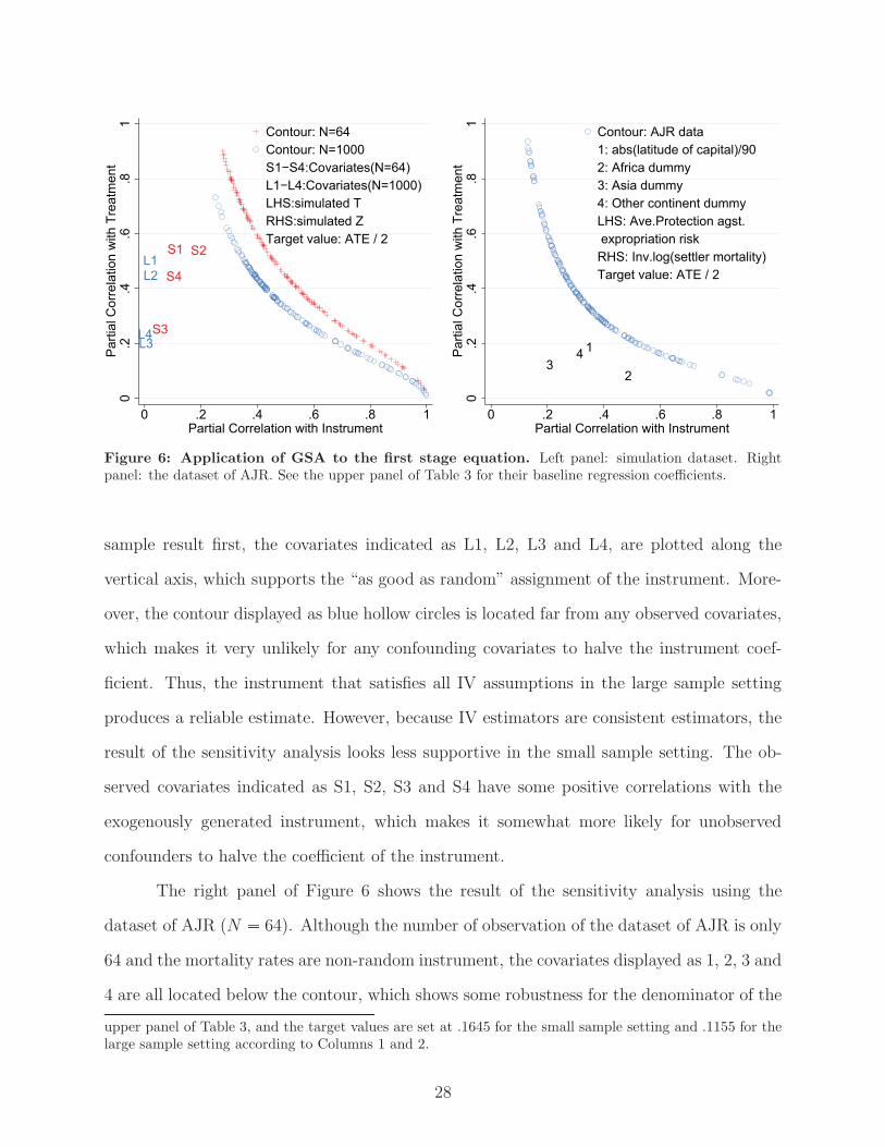
L1L2

L3L4

S1 S2

S3

S4

0.2

.4.6

.81

Par

tial C

orre

latio

n w

ith T

reat

men

t

0 .2 .4 .6 .8 1Partial Correlation with Instrument

Contour: N=64Contour: N=1000S1−S4:Covariates(N=64)L1−L4:Covariates(N=1000)LHS:simulated TRHS:simulated ZTarget value: ATE / 2

1

23

4

0.2

.4.6

.81

Par

tial C

orre

latio

n w

ith T

reat

men

t

0 .2 .4 .6 .8 1Partial Correlation with Instrument

Contour: AJR data1: abs(latitude of capital)/902: Africa dummy3: Asia dummy4: Other continent dummyLHS: Ave.Protection agst. expropriation riskRHS: Inv.log(settler mortality)Target value: ATE / 2

Figure 6: Application of GSA to the first stage equation. Left panel: simulation dataset. Rightpanel: the dataset of AJR. See the upper panel of Table 3 for their baseline regression coefficients.

sample result first, the covariates indicated as L1, L2, L3 and L4, are plotted along the

vertical axis, which supports the “as good as random” assignment of the instrument. More-

over, the contour displayed as blue hollow circles is located far from any observed covariates,

which makes it very unlikely for any confounding covariates to halve the instrument coef-

ficient. Thus, the instrument that satisfies all IV assumptions in the large sample setting

produces a reliable estimate. However, because IV estimators are consistent estimators, the

result of the sensitivity analysis looks less supportive in the small sample setting. The ob-

served covariates indicated as S1, S2, S3 and S4 have some positive correlations with the

exogenously generated instrument, which makes it somewhat more likely for unobserved

confounders to halve the coefficient of the instrument.

The right panel of Figure 6 shows the result of the sensitivity analysis using the

dataset of AJR (N � 64). Although the number of observation of the dataset of AJR is only

64 and the mortality rates are non-random instrument, the covariates displayed as 1, 2, 3 and

4 are all located below the contour, which shows some robustness for the denominator of the

upper panel of Table 3, and the target values are set at .1645 for the small sample setting and .1155 for thelarge sample setting according to Columns 1 and 2.

28

Wald estimator. However, it must be kept in mind that these covariates have moderately

strong correlations with the instrument, which violates one of the IV assumptions of “as

good as random” assignment of the instrument.

Sensitivity analysis to the reduced form equation. The reduced-form equation re-

gresses the outcome on the instrument and other observed covariates, and the sensitivity

analysis is set up as follows.

logpgp95 � τ2logem4 � xβ2 � δ2u� ε2 (27)

logem4 � xγ2 � α2u� υ2 (28)

where logpgp95 is the outcome, logged GDP per capita in 1995, τ2 is the coefficient of the

instrument on the outcome, β2 and γ2 are a vector of the coefficients, α2 and δ2 are sensitivity

parameters, and ε2 and υ2 are error terms.

In the Wald estimator, τ2 is the numerator. Therefore, if τ2 is not robust against the

omitted exogenous unobservable, the Wald estimate will be unreliable. The result of the

sensitivity analysis is presented in the left panel of Figure 7.32 In the figure, the sensitivity

analysis is performed in the small sample setting (displayed as green triangles) and the large

sample settings (displayed as blue hollow circles). For comparison, the sensitivity analysis

is also performed to the naive outcome model (i.e. the regression of the outcome on the

un-instrumented treatment; displayed as red crosses).

In the large sample setting, the partial correlations of the covariates (LZ1, LZ2, LZ3

and LZ4) are plotted near the vertical axis. This makes it very unlikely that any unobserved

confounder has confounding effects as strong as those displayed as blue hollow circles. In

the small sample setting, the covariates (SZ1, SZ2, SZ3 and SZ4) have weak correlations

with the instrument, which makes the IV estimates somewhat unreliable. On the other

32The regression estimates of the reduced-form equation with the simulation dataset are reported in theupper panel of Table 3, and the target values are set at .0935 for the small sample setting and .061 for thelarge sample setting according to Columns 5 and 6.

29

SZ1

SZ2

SZ3

SZ4

LZ1

LZ2

LZ3

LZ4

LT1

LT2

LT3

LT4

0.2

.4.6

.81

Par

tial C

orre

latio

n w

ith O

utco

me

0 .2 .4 .6 .8 1Partial Correlation with Treatment / IV

Contour: RHS=T,N=1000Contour: RHS=Z,N=64Contour: RHS=Z,N=1000LT1−4:Covariates(RHS=T,N=1000)SZ1−4:Covariates(RHS=Z,N=64)LZ1−4:Covariates(RHS=Z,N=1000)LHS:simulated YTarget value: ATE / 2

Z1

Z2

Z3

Z4

T1

T2

T3

T4

0.2

.4.6

.81

Par

tial C

orre

latio

n w

ith O

utco

me

0 .2 .4 .6 .8 1Partial Correlation with Treatment / IV

Contour: naive reg.Contour: reduced form eq.T1−4:Covariates(naive reg.)Z1−4:Covariates(reduced form)1: abs(latitude of capital)/902: Africa dummy3: Asia dummy4: Other continent dummyLHS:ln(GDP per capita)

Figure 7: Application of GSA to the reduced form equation. Left panel: simulation dataset. Rightpanel: the dataset of AJR. See the lower panel of Table 3 for their baseline regression coefficients.

hand, the result of the sensitivity analysis to the naive outcome model show that most of

the partial correlations of the covariates (LT1, LT2, LT3 and LT4) are plotted above the

contour displayed as red crosses, which indicates that the naive estimate is not robust against

omitted confounders.

Furthermore, the comparison of the partial correlations of the observed covariates

between the reduced form equation and the naive outcome model in the large sample setting

also highlights interesting commonality between this application and the applications to

other quasi-experimental techniques. Specifically, each plot of the partial correlations shifts

to the left between the naive outcome model and the reduced form equation (e.g. LZ1 �

LT1). Thus, the result implies that introduction of an instrument makes the IV estimator

more robust against unobserved confounders by making the treatment more independent of

other covariates.

The right panel of Figure 7 presents the results of the sensitivity analysis with the

dataset of AJR. According to Columns 2 and 3 of Table 3, the target values are set at .227

for the reduced form equation (displayed as blue hollow circles) and .2825 for the naive

30

outcome model (displayed as red crosses) . The partial correlations of the covariates in the

reduced-form equation (Z1, Z2, Z3 and Z4) are at least as large as those in the naive outcome

model (T1, T2, T3 and T4). Furthermore, Africa dummy (Z2) is plotted near the contour

displayed as blue hollow circles. This implies that an unobserved confounder as strong as

those of Africa dummy can halve the coefficient of the instrument. Given that some of the

covariates appear in AJR such as British colonial dummy have stronger partial effects than

Africa dummy, this is fairly likely. Thus, the introduction of the settler’s mortality rate as

IV does not seem to improve the robustness of the numerator of the Wald estimator against

the unobserved confounding.

To sum up, when robustness is defined in terms of the possibility that the Wald

estimator either doubles or is halved, the estimation strategy by AJR is not supported as a

way to produce a reliable IV estimator because of the lack of robustness in the numerator

of the Wald estimate.

8 Concluding remarks

In this paper, I have introduced GSA and demonstrated its versatility and simplicity of

use through its application to various quasi-experimental methods. As is the case with the

development of matching techniques, various sensitivity analyses have been proposed, and

each of them has unique strength. I believe GSA should be added as one of such methods

if not dominates other methods. Above all, GSA allows researchers to set the target value

in terms of test statistics and to assume any combination of the link functions requiring

minimal changes to the researchers’ original estimation models.

The applications of GSA to fixed effects model, propensity score matching, and instru-

mental variable approach show that successful applications of quasi-experimental techniques

make the treatment assignment less dependent on the covariates as well as unobserved con-

founders. Unlike regression tables or conventional tests, GSA visualizes this process by

showing the reduction in the partial correlation between the treatment and the covariates

31

relative to the necessary confounding to change the treatment effect by a given amount.

Finally, the sensitivity analysis is still a developing field and requires further research

particularly in development of reliable benchmark, which could be improved in two aspects.

First, the researchers’ substantive knowledge about the treatment effect needs to be incor-

porated into the sensitivity analysis in evaluating the contour or in setting the target value.

This would be particularly useful in some research fields where a certain size of the treatment

effect is widely known such as economic return to education. Second, the objective criteria

to evaluate the contour needs to be developed. Inventing a new test statistics would be

challenging but promising effort.

References

Acemoglu, D., S. Johnson & J.A. Robinson. 2001. “The Colonial Origins of Comparative

Development: An Empirical Investigation.” American Economic Review .

Albouy, David Yves. 2012. “The Colonial Origins of Comparative Development: An Empir-

ical Investigation: Comment.” American Economic Review 102(6):pp. 3059–3076.

Altonji, J.G., T.E. Elder & C.R. Taber. 2005. “Selection on observed and unobserved vari-

ables: Assessing the effectiveness of Catholic schools.” Journal of Political Economy

113(1):151–184.

Angrist, J.D. 1990. “Lifetime earnings and the Vietnam era draft lottery: evidence from

social security administrative records.” The American Economic Review pp. 313–336.

Angrist, J.D. & J.S. Pischke. 2008. Mostly harmless econometrics: An empiricist’s compan-

ion. Princeton University Press.

Angrist, Joshua D., Guido W. Imbens & Donald B. Rubin. 1996. “Identification of Causal

Effects Using Instrumental Variables.” Journal of the American Statistical Association

91(434):pp. 444–455.

32

Becker, S.O. & M. Caliendo. 2007. “Sensitivity analysis for average treatment effects.” Stata

Journal 7(1):71.

Bingenheimer, J.B., R.T. Brennan & F.J. Earls. 2005. “Firearm violence exposure and

serious violent behavior.” Science 308(5726):1323–1326.

Blattman, C. 2009. “From Violence to Voting: War and political participation in Uganda.”

American Political Science Review 103(2):231–247.

Caughey, DM& JS Sekhon. 2012. “Elections and the regression-discontinuity design: Lessons

from us house races, 1942-2008.” Political Analysis .

Clarke, K.A. 2005. “The phantom menace: Omitted variable bias in econometric research.”

Conflict Management and Peace Science 22(4):341–352.

Dehejia, R.H. & S. Wahba. 2002. “Propensity score-matching methods for nonexperimental

causal studies.” Review of Economics and Statistics 84(1):151–161.

Fearon, J.D. & D.D. Laitin. 2003. “Ethnicity, insurgency, and civil war.” American political

science review 97(1):75–90.

Heckman, J., H. Ichimura, J. Smith & P. Todd. 1998. “Characterizing selection bias using

experimental data.” Econometrica pp. 1017–1098.

Hill, Jennifer. 2008. “Comment on “Can nonrandomized experiments yield accurate answers?

A randomized experiment comparing random and nonrandom assignments” by Shadish,

Clark, and Steiner.” Journal of the American Statistical Association 103(484):1346–

1350.

Ho, D.E., K. Imai, G. King & E.A. Stuart. 2007. “Matching as nonparametric preprocess-

ing for reducing model dependence in parametric causal inference.” Political Analysis

15(3):199–236.

33

Horowitz, D.L. 1985. Ethnic groups in conflict. University of California press, Berkeley, CA.

Ichino, Andrea, Fabrizia Mealli & Tommaso Nannicini. 2008. “From temporary help jobs

to permanent employment: What can we learn from matching estimators and their

sensitivity?” Journal of Applied Econometrics 23(3):305–327.

Imai, K., L. Keele, D. Tingley & T. Yamamoto. 2011. “Unpacking the black box of causal-

ity: Learning about causal mechanisms from experimental and observational studies.”

American Political Science Review 105(4):765–789.

Imai, K. & T. Yamamoto. 2010. “Causal inference with differential measurement error:

Nonparametric identification and sensitivity analysis.” American Journal of Political

Science 54(2):543–560.

Imbens, Guido W. 2003. “Sensitivity to Exogeneity Assumptions in Program Evaluation.”

The American Economic Review 93(2):126–132.

Imbens, Guido W. & Jeffrey M. Wooldridge. 2009. “Recent Developments in the Economet-

rics of Program Evaluation.” Journal of Economic Literature 47(1):5–86.

LaLonde, R.J. 1986. “Evaluating the econometric evaluations of training programs with

experimental data.” The American Economic Review 76(4):604–620.

Leuven, Edwin & Barbara Sianesi. 2003. “PSMATCH2: Stata module to perform full Ma-

halanobis and propensity score matching, common support graphing, and covariate

imbalance testing.” Statistical Software Components, Boston College Department of

Economics.

Manpower, Demonstration Research Corporation. N.d. National Supported Work Evaluation

Study, 1975-1979 [ICPSR07865]. Inter-university Consortium for Political and Social

Research, Ann Arbor, MI.

34

McKelvey, R.D. & W. Zavoina. 1975. “A statistical model for the analysis of ordinal level

dependent variables.” Journal of Mathematical Sociology 4(1):103–120.

Rosenbaum, Paul R. 2005. Sensitivity Analysis in Observational Studies. In Encyclopedia of

Statistics in Behavioral Science. John Wiley & Sons, Ltd.

Rosenbaum, P.R. 2002. Observational studies. Springer Verlag.

Rosenbaum, P.R. & D.B. Rubin. 1983. “The central role of the propensity score in observa-

tional studies for causal effects.” Biometrika 70(1):41–55.

Rubin, D.B. 1978. “Bayesian inference for causal effects: The role of randomization.” The

Annals of Statistics pp. 34–58.

Smith, J. A. & P. E. Todd. 2005. “Does matching overcome LaLonde’s critique of nonex-

perimental estimators?” Journal of Econometrics 125(1-2):305–353.

Sobel, Michael E. 2012. “Does Marriage Boost Men’s Wages?: Identification of Treatment

Effects in Fixed Effects Regression Models for Panel Data.” Journal of the American

Statistical Association 107(498):521–529.

StataCorp. 2011. Stata 12 Base Reference Manual. Stata Press, College Station, TX.

Stock, J.H. & M. Yogo. 2002. “Testing for weak instruments in linear IV regression.”.

University, of Michigan, National Science Foundation National Institute of Aging Institute

of Child Health & Human Development. 1978. Panel Study of Income Dynamics, public

use dataset. University of Michigan, Ann Arbor, MI.

Wooldridge, J.M. 2009. Introductory econometrics: A modern approach. South-Western

Pub.

?

35

A Checking the performance of GSA through Monte Carlo sim-

ulation

In this section, statistical properties of GSA are explored through Monte Carlo simulations.

We are particularly interested in how well GSA recovers the true treatment effect when

researchers know true sensitivity parameters. As a basis of comparison, the results obtained

from Imbens’ (2003) sensitivity analysis (henceforth Imbens’ SA) are used. This method has

been widely used as a forerunner of dual parameter sensitivity analysis.33

To overview the results, GSA yields less biased treatment effects when the sensi-

tivity parameter of the treatment model is extreme though both GSA and Imbens’ SA

unbiasedly estimate the true treatment effects, otherwise. When the sensitivity parameter

of the outcome model is extreme, Imbens’ SA is slightly more efficient in estimating the

population-level treatment effects than GSA, while GSA yields more efficient sample-level

treatment effects than Imbens’ SA. The two methods particularly disagree in the estimation

of standard errors (SEs). Specifically, GSA yields the SE estimates when a true unobserved

confounder (U) is included in the model, while Imbens’ SA yields the SE estimates when

a pseudo unobservable (PU) is included in the model. I will discuss later why the former

quantities are more important for the sensitivity analysis.

First, let us overview how the two methods are different using LaLonde’s (1986)

experimental dataset. In Figure 8, the horizontal and vertical axes represent α and δ, which

are raw coefficients of PUs. The estimated contours from Imbens’ SA are displayed as red

solid line, and the scatter plots from GSA are displayed as blue hollow circles. The left

figure, which shows the sets of the sensitivity parameters that lower the treatment effect

by $1,000, indicates that the scatter plots obtained from GSA overlap with the red contour

curve obtained from Imbens’ SA. That is, both approaches identify the same (and correct)

confounding effects that change the treatment effects by a given amount.

On the other hand, the right figure, which shows the sets of the sensitivity parameters

33See Clarke (2005) and Blattman (2009) for the early application of Imbens’ SA.

36

13

57

delta

0 2 4alpha

Target value: coefficient

01

23

45

delta

0 1 2 3alpha

Target value: -valuet

Figure 8: Comparison between GSA and Imbens’ SA approach when the target value iscoefficient(left) and t-value(right).

that lower the t-value of the treatment effect from 2.606 to 1.645 (i.e. 10% significance level),

shows that two methods identify different sets of sensitivity parameters. Specifically, GSA

provides larger sensitivity parameters than Imbens’ SA in the upper left, and smaller ones

in the lower right. In the following, I will present the results of Monte Carlo simulations and

discuss the practical considerations regarding this discrepancy.

Simulation design. GSA and Imbens’ SA are compared through Monte Carlo simulation.

First, the dataset is generated following Imbens’ (2003) original setting. That is, the identity

link function is assumed for the outcome model, the logistic link function is assumed for the

treatment model, and a binary unobserved confounder is assumed. The data generating

37

process (DGP) is:

X1, X2, X3 � Normal�0, 1� (29)

U � Binomial�1, .5� (30)

Z� � Λ�.4X1 � .3X2 � .2X3 � α�U � .5�� (31)

Z � Binomial�1, Z�� (32)

ε � Normal�0, 1� (33)

Y0 � 0� .5X1 �X2 � 1.5X3 � δU � ε (34)

Y1 � 2� .5X1 �X2 � 1.5X3 � δU � ε (35)

Y � Y0 � �1� Z� � Y1 � Z (36)

where X1, X2 and X3 are observed covariates, U is a binary true unobserved confounder,34

Z� is a propensity score, Λ is inverse logit function, Z is a binary treatment variable, ε

is a stochastic disturbance term, Y0 and Y1 are the potential outcome, Y is an outcome

variable, and α and δ are sensitivity parameters. α and δ take the value of either 0, 2, or 4

respectively. Thus, the simulations are performed under nine different confounding effects.

The true estimation models for the outcome and the treatment models in a given dataset

are stated as follows.

E�y�z, x1, x2, x3, u� � β0 � β1x1 � β2x2 � β3x3 � τ z � δu (37)

E�z�x1, x2, x3, u� � Λ�γ0 � γ1x1 � γ2x2 � γ3x3 � αu� (38)

Second, GSA and Imbens’ SA are performed to the dataset. With researchers’ knowl-

edge about true sensitivity parameters, GSA attempts to recover u and the treatment effects

34Note that we must use a binary U because Imbens’ SA cannot deal with a continuous U . However,the use of a binary U puts GSA at a disadvantage because GSA’s orthogonality condition between X andU is better satisfied with a continuous U . In other words, the estimated treatment coefficient and standarderror obtained using a binary U are less precise than those obtained using a continuous U due to empiricalcorrelation between a binary U and X .

38

with the following models, which simply replace u with pu.35

E�y�z, x1, x2, x3, pu� � β0 � β1x1 � β2x2 � β3x3 � τ z � δpu (39)

E�z�x1, x2, x3, pu� � Λ�γ0 � γ1x1 � γ2x2 � γ3x3 � αpu� (40)

Imbens’ SA yields the treatment effect by maximizing the likelihood function of the above

models and by integrating the marginal probability of U in the function. Note that we

can suppose two different situations of what researchers know about the “true” sensitivity

parameters. In one situation, researchers know the population-level confounding effects

of U , or the coefficients of U used in DGP. In the other situation, researchers know the

confounding effects of U in a given dataset, or α and δ in Equations (37) and (38). Although

all simulations are performed under these two different assumptions, they do not make

notable differences. Thus, I present the results obtained with population-level sensitivity

parameters when the statistics represent population-level properties and those obtained with

sample-level sensitivity parameters when the statistics represent sample-level properties.

Third, the simulation is iterated 1,000 times for each of 9 distinct specifications of

the sensitivity parameters. The performances of GSA and Imbens’ SA are evaluated accord-

ing to the following two criteria. The first criterion is how accurately sensitivity analysis

recovers population parameters of the treatment. The root-mean-square error (RMSE) of

the estimated coefficient with respect to τ

���1�1000

�1000

i�1 �τi � τ�2�

and the RMSE

of the estimated standard errors with respect to the standard deviation of the estimated

coefficients

���

1�1000�1000

i�1 �SE�τi� � SD�τ��2�

are used as benchmark combined with

the sensitivity parameters at population level. The other criterion is how accurately sen-

sitivity analysis recovers the estimates that would be obtained if a true U were observed.

With this criterion, the root-mean-square deviations (RMSDs) between the estimated coeffi-

cient and τ

���

1�1000�1000

i�1 �τi � τi�2

�and the estimated standard errors against SE�τ�

35A wrapper program of GSA that enables users to set α and δ is developed to run this simulation.

39

���1�1000

�1000

i�1 �SE�τi� � SE�τi��2

�are used as benchmark combined with the sensitiv-

ity parameters at sample level.

Simulation results. The simulation results are presented from Table 4 to Table 9. For

each distinct combination of the sensitivity parameters, the results of GSA are presented in

the left column and those of Imbens’ SA are presented in the right column. First, let us take a

look at the basic statistics. For these results, the population-level sensitivity parameters are

assumed to be known. That is, α and δ in the tables are used as-is. Table 4 shows the mean

of the estimated treatment effect over 1,000 iterations. Both methods slightly overestimate

the treatment coefficients when the sensitivity parameter in the treatment model (α) is set

at an extremely large value (i.e. α � 4), but the bias of the GSA is smaller than that

of Imbens’ SA. Imbens’ SA yields the treatment effect estimates for a wide range of the

sensitivity parameters even when GSA fails to generate PUs. This allows researchers to

obtain extended contours, while the estimates obtained in such cases are typically erroneous

as indicated by the simulation results. Both methods, otherwise, unbiasedly estimate the

treatment effects as long as correct sensitivity parameters are provided.

On the other hand, the two methods return quite different estimates for the standard

errors (SEs).36 In a simple regression of Y on Z and U , the SE of the treatment coeffi-

cient is expressed as SE�Z� � �Z��1� corr�Z, U�

�, where σ is a residual variance and

corr�Z, U� is the correlation between Z and U . The larger α implies the larger corr�Z, U�

and the larger SE estimates. Table 5 shows that as α becomes larger the estimated SEs

obtained from GSA becomes larger, while the counterparts for Imbens’ SA becomes smaller.

The SE estimates of Imbens’ SA change this way because they represent the dispersion of τ

in the sensitivity analysis not the dispersion of τ in the true model. The difference between

these two dispersions reflect the fact that, as α becomes larger, the more limited numbers

36The average SEs are calculated as the square root of the average of the squared standard errors over1,000 iterations.

40

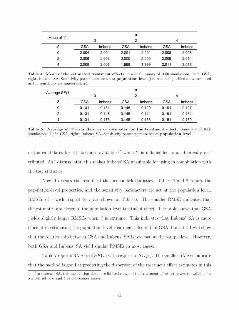
Table 4: Mean of the estimated treatment effects. τ � 2. Summary of 1000 simulations. Left: GSA,right: Imbens’ SA. Sensitivity parameters are set at population level (i.e. α and δ specified above are usedas the sensitivity parameters as-is).

Table 5: Average of the standard error estimates for the treatment effect. Summary of 1000simulations. Left: GSA, right: Imbens’ SA. Sensitivity parameters are set at population level.

of the candidates for PU becomes available,37 while U is independent and idnetically dis-

tributed. As I discuss later, this makes Imbens’ SA unsuitable for using in combination with

the test statistics.

Now, I discuss the results of the benchmark statistics. Tables 6 and 7 report the

population-level properties, and the sensitivity parameters are set at the population level.

RMSEs of τ with respect to τ are shown in Table 6. The smaller RMSE indicates that

the estimates are closer to the population-level treatment effect. The table shows that GSA

yields slightly larger RMSEs when δ is extreme. This indicates that Imbens’ SA is more

efficient in estimating the population-level treatment effects than GSA, but later I will show

that the relationship between GSA and Imbens’ SA is reversed at the sample level. However,

both GSA and Imbens’ SA yield similar RMSEs in most cases.

Table 7 reports RMSEs of SE�τ � with respect to SD�τ�. The smaller RMSEs indicate

that the method is good at predicting the dispersion of the treatment effect estimates in this

37In Imbens’ SA, this means that the more limited range of the treatment effect estimates is available fora given set of α and δ as α becomes larger.

41

Table 6: RMSE of the treatment effect estimates with respect to the true treatment effect.Summary of 1000 simulations. Left: GSA, right: Imbens’ SA. Sensitivity parameters are set at populationlevel.

Table 7: RMSE of the SE estimates of the treatment effect with respect to the SD of thetreatment effect estimates. Summary of 1000 simulations. Left: GSA, right: Imbens’ SA. Sensitivityparameters are set at population level.

simulation. Unlike Table 6, Table 7 shows that RMSEs of Imbens’ SA are much smaller than

the counterparts of GSA. This, however, does not mean GSA yields nonsensical estimates. I

show later that GSA’s SE estimates represent the dispersion of the treatment effect estimates

when true Us are observed.

Tables 8 and 9 are similar to Tables 6 and 7, but the sensitivity parameters are set at

the sample level. That is, estimated coefficients of U (δ in Equation (37) and α in Equation

(38)) in a dataset corresponding to one of nine combinations of α and δ are used in DGP.

The following two tables also report the statistics that measure its sample-level performance.

Table 8 shows RMSDs between τ and τ . This quantity represents the average devi-

ation of the treatment effect estimates from the counterparts that would be obtained if true

Us were observed. Both methods yield small RMSDs when the sensitivity parameter in the

outcome model (δ) is not extreme, but Imbens’ SA yields large RMSDs when δ is extreme.

In contrast to Table 6, this indicates that GSA estimates the sample-level treatment effects

more efficiently than Imbens’ SA. In general, Tables 6 and 8 indicates that two methods

42

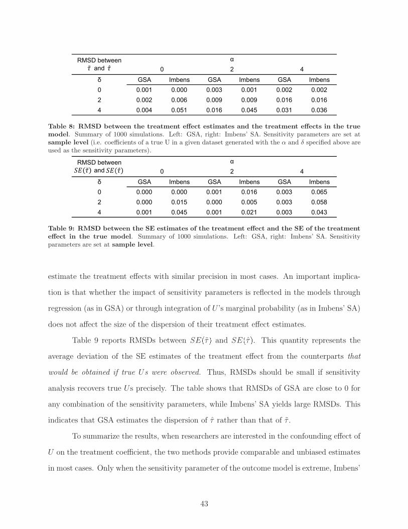
Table 8: RMSD between the treatment effect estimates and the treatment effects in the truemodel. Summary of 1000 simulations. Left: GSA, right: Imbens’ SA. Sensitivity parameters are set atsample level (i.e. coefficients of a true U in a given dataset generated with the α and δ specified above areused as the sensitivity parameters).

Table 9: RMSD between the SE estimates of the treatment effect and the SE of the treatmenteffect in the true model. Summary of 1000 simulations. Left: GSA, right: Imbens’ SA. Sensitivityparameters are set at sample level.

estimate the treatment effects with similar precision in most cases. An important implica-

tion is that whether the impact of sensitivity parameters is reflected in the models through

regression (as in GSA) or through integration of U ’s marginal probability (as in Imbens’ SA)

does not affect the size of the dispersion of their treatment effect estimates.

Table 9 reports RMSDs between SE�τ� and SE�τ�. This quantity represents the

average deviation of the SE estimates of the treatment effect from the counterparts that

would be obtained if true Us were observed. Thus, RMSDs should be small if sensitivity

analysis recovers true Us precisely. The table shows that RMSDs of GSA are close to 0 for

any combination of the sensitivity parameters, while Imbens’ SA yields large RMSDs. This

indicates that GSA estimates the dispersion of τ rather than that of τ .

To summarize the results, when researchers are interested in the confounding effect of

U on the treatment coefficient, the two methods provide comparable and unbiased estimates

in most cases. Only when the sensitivity parameter of the outcome model is extreme, Imbens’

43

SA is better at estimating the population-level treatment effects, while GSA is better at

estimating the sample-level treatment effects. Also, when the sensitivity parameter of the

treatment model is extreme, GSA yields less biased estimates. When neither of the sensitivity

parameters is extreme, the two methods yield comparable estimates. Then, Imbens’ SA is

computationally more efficient.

When researchers are interested in the confounding effect of U on the test statistics

of the treatment, I argue that GSA is more appropriate than Imbens’ SA. In short, what

researchers want to know is the impact of U not PU. The SE estimates of GSA approximate

the SEs when the models include true Us, while the SE estimates of Imbens’ SA are precise

but represent the dispersion of the estimates when the models include PUs. As we have seen

in Table 5, U and PU have different properties regarding their impacts on SE estimates.

Thus, researchers should use GSA when test statistics are used as the target value. Finally,

it must be noted that GSA produces more precise estimates when U is assumed to be

continuous than when U is binary. A binary U is assumed in this simulation because Imbens’

SA cannot deal with continuous U .

B Procedure of Generalized Sensitivity Analysis

This section describes the procedure of GSA in more detail. Figure 1 presents the overview.

For the sake of clarity, I consider the following linear models, but GSA is compatible with

the models with various link functions.

Zi � γ�Xi � αUi � εi (41)

Yi � τZi � β �Xi � δUi � εi (42)

where Yi is an outcome variable, Zi is a treatment variable, Xi is a vector of observed covari-

ates, Ui is an unobserved covariate which is orthogonal to Xi, α, β, γ and δ are coefficients,

and εi and εi are error terms. GSA also assumes stable unit treatment value assumption,

44

which requires the independence of the treatment assignment process from individual-level

treatment status. In sensitivity analysis, researchers are interested in the substantive size

and/or statistical significance of the treatment effect, as well as the coefficients of the un-

observed confounder, α and δ, that change the sizes of the treatment effect to some target

value.

1. Define the quantity of interest, decide its target size, and save the partial

effects of the original models. The quantity of interest is usually defined in terms of

either test statistics or coefficient of the treatment variable. If researchers are concerned

about the size of confounding due to an unobserved confounder that turns a positive and

statistically significant treatment effect into an insignificant one, they may want to define

their quantity of interest as the t-statistics of the treatment effect and set the target value

at one of the critical values (e.g. 1.645 or 1.96) or a value slightly smaller than that. On the

other hand, if researchers are concerned about the confounding effect on the substantive size

of the treatment effect, the quantity of interest should be defined in terms of the coefficient

of the treatment variable and set the target value accordingly.

Because the coefficients of an unobserved confounder, or the two sensitivity param-

eters, α and δ, have no substantive meaning per se, they are often transformed into other

forms of partial effects. For instance, Imbens (2003) suggests converting α and δ to the par-

tial R-squares of an unobserved confounder in the treatment assignment equation�R2

Z,par

�

and the partial R-square in the outcome equation�R2

Y,par

�respectively. To calculate the

partial R-squares, the R-squares in the original models�R2

Z,o and R2Y,o

�must be recorded

beforehand. This process is not necessary if researchers convert α and δ to partial correla-

tions.

2. Generate a candidate variable for a PU. Next, a pseudo unobservable (PU) is

generated through the following process, and this is the most important part of GSA. First,

an initial intermediate unobservable, �U , is generated from a weighted average of residuals

45

from treatment and outcome models plus random noise:

�U � N �c1 � dz � c2 � dy, 1� (43)

where �U is an intermediate random variable drawn from the normal distribution with the

mean of c1 � dz � c2 � dy and a unit variance, c1 and c2 are the key location parameters, and

dy and dz are the standardized deviance residuals from Equations (10) and (11).38 Then, a

second intermediate variable, �U , is obtained by residualizing the first intermediate variable

by X:

�U � �U � �λ�X, where �λ � argminλ

� �U � λ�X� (44)

where λ is a vector of regression coefficients. Then, the second intermediate random vari-

able, �U , is adopted as a candidate variable, U , only if it is approximately orthogonal to

the observed covariates (Equation (7)).39 When a PU is assumed to be a binary, the third

intermediate variable is created from the second intermediate variable, �U , by dichotomizing

�U at its median. Then, whether this binary third intermediate variable satisfies the orthog-

onality condition is checked. Because this process requires a greater number of iterations

particularly with a small number of observations, the use of a binary PU should be avoided

unless researchers have a strong reason to do so.40

As seen in the lower left plots displayed as red hollow circles in Figure 9, a candidate

variable generated from a purely random variable can take only a limited range of α and

δ. Thus, GSA indirectly adjusts the sizes of two sensitivity parameters, α and δ through

the manipulation of the two location parameters, c1 and c2. Because dz is associated with

the unexplained variations in the treatment model, the larger the c1, the larger the α as

displayed as blue hollow diamonds in the lower right of Figure 9. Likewise, the larger the c2,

38See p.619 of Stata Base Reference for the list of the deviation residuals of different families.39A reasonable error tolerance level for the orthogonality condition will be discussed later.40For example, researchers may have a concrete idea about a binary unobserved confounder such as a

gene. Also, a binary PU needs to be assumed to compare the results of GSA with those of Imbens’ (2003)approach.

46

-.5

0.5

11

.5d

elta

-1 0 1 2 3alpha

c1=0;c =12 c1=1;c =12

c1=0;c =02 c1=1;c =02

Figure 9: Distribution of a candidate variable of a PU with different data generation processes.

the larger the δ (in yellow hollow triangles in the lower right of Figure 9).

3. Adopt a candidate variable, U , as a PU if the size of the estimand is close

enough to the target value. Otherwise, repeat to Step 2. Model (8) is estimated

replacing U with a candidate variable, U , and U is adopted as a PU, U , if the estimand is

close enough to the target value. For example, when the target value is t � 1.96 and the

error tolerance level is 1%, a candidate variable is accepted as a PU if the test statistics of

the model with the candidate variable is 1.94 � t � 1.98.41 If the difference between the

estimand and the target value is more than the error tolerance level, this candidate variable

is discarded, and it will be regenerated until a PU is found. The iteration algorithm is

discussed in detail in Appendix C.

Note: Two screening processes in making PUs. Step 2 and Step 3 involves the

two screening processes that make PUs closer to what they are theoretically assumed. The

first mechanism is the orthogonalization. That is, a second intermediate random variable,

�U , is adopted as a candidate variable, U , only if it satisfies the orthogonality condition in

Equation (7). Of course, with real data, a random variable can never be perfectly orthogonal

41An optimal error tolerance level is discussed later in this section.

47

to covariates. Thus, we must set a reasonable error tolerance level that is sufficiently strict

so that the violation of the assumption in Equation (7) is negligible yet not too strict to

generate candidate variables becomes nearly impossible.

Specifically, GSA checks the orthogonality of an intermediate random variable in

the following way. First, the treatment model is estimated including a second intermediate

random variable ( �U) in the right hand side:

E�Z� � g�1z

�X�γ � �α �U

�(45)

where �γ and �α are the estimates obtained from Equation (45). If �U is orthogonal to X,

the coefficients of X obtained from Equation (45), �γ, should not be different from those

obtained from the model without U (i.e. γ in Equation (11)). Thus, the correlation between

the vector of regression values of X in Equation (45), X�γ, and the counterpart in Equation

(11), Xγ, should be close to unity. Thus, the first check is set up as follows:42

U � �U if ρ�X�γ,Xγ� � ρthreshold (46)

where ρ is the correlation coefficient and ρthreshold is a threshold level of the correlation

coefficient (e.g. 0.99).

The second mechanism is to accept a candidate variables as a PU only if its con-

founding effect changes the treatment effect close to the target value. Formally,

PU � U if �qoi� qoitarget� � εthreshold (47)

where qoi is a quantity of interest such as treatment effect coefficient or t-statistics and

εthreshold is an error tolerance level (e.g. 0.01).

A simple simulation was performed to examine the extent to which these screening

42�U must be standardized

48

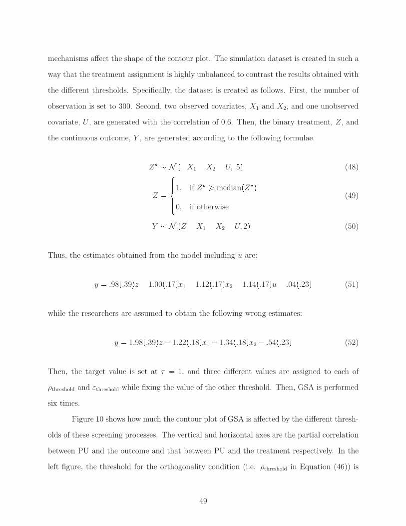
mechanisms affect the shape of the contour plot. The simulation dataset is created in such a

way that the treatment assignment is highly unbalanced to contrast the results obtained with

the different thresholds. Specifically, the dataset is created as follows. First, the number of

observation is set to 300. Second, two observed covariates, X1 and X2, and one unobserved

covariate, U , are generated with the correlation of 0.6. Then, the binary treatment, Z, and

the continuous outcome, Y , are generated according to the following formulae.

Z� � N ��X1 �X2 � U, .5� (48)

Z �

�������1, if Z� � median�Z��

0, if otherwise

(49)

Y � N �Z �X1 �X2 � U, 2� (50)

Thus, the estimates obtained from the model including u are:

y � .98�.39�z � 1.00�.17�x1 � 1.12�.17�x2 � 1.14�.17�u� .04�.23� (51)

while the researchers are assumed to obtain the following wrong estimates:

y � 1.98�.39�z � 1.22�.18�x1 � 1.34�.18�x2 � .54�.23� (52)

Then, the target value is set at τ � 1, and three different values are assigned to each of

ρthreshold and εthreshold while fixing the value of the other threshold. Then, GSA is performed

six times.

Figure 10 shows how much the contour plot of GSA is affected by the different thresh-

olds of these screening processes. The vertical and horizontal axes are the partial correlation

between PU and the outcome and that between PU and the treatment respectively. In the

left figure, the threshold for the orthogonality condition (i.e. ρthreshold in Equation (46)) is

49

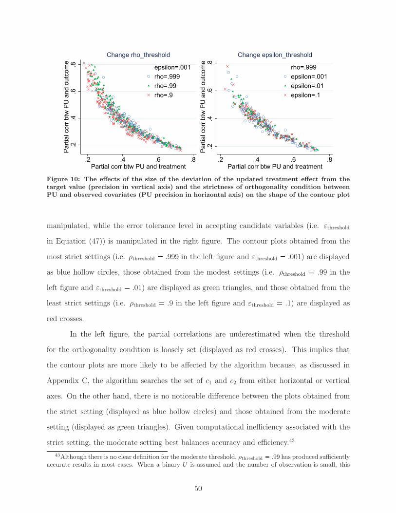
.2.4

.6.8

Par

tial c

orr b

tw P

U a

nd o

utco

me

.2 .4 .6 .8Partial corr btw PU and treatment

epsilon=.001rho=.999rho=.99rho=.9

Change rho_threshold

.2.4

.6.8

Par

tial c

orr b

tw P

U a

nd o

utco

me

.2 .4 .6 .8Partial corr btw PU and treatment

rho=.999epsilon=.001epsilon=.01epsilon=.1

Change epsilon_threshold

Figure 10: The effects of the size of the deviation of the updated treatment effect from thetarget value (precision in vertical axis) and the strictness of orthogonality condition betweenPU and observed covariates (PU precision in horizontal axis) on the shape of the contour plot

manipulated, while the error tolerance level in accepting candidate variables (i.e. εthreshold

in Equation (47)) is manipulated in the right figure. The contour plots obtained from the

most strict settings (i.e. ρthreshold � .999 in the left figure and εthreshold � .001) are displayed

as blue hollow circles, those obtained from the modest settings (i.e. ρthreshold � .99 in the

left figure and εthreshold � .01) are displayed as green triangles, and those obtained from the

least strict settings (i.e. ρthreshold � .9 in the left figure and εthreshold � .1) are displayed as

red crosses.

In the left figure, the partial correlations are underestimated when the threshold

for the orthogonality condition is loosely set (displayed as red crosses). This implies that

the contour plots are more likely to be affected by the algorithm because, as discussed in

Appendix C, the algorithm searches the set of c1 and c2 from either horizontal or vertical

axes. On the other hand, there is no noticeable difference between the plots obtained from

the strict setting (displayed as blue hollow circles) and those obtained from the moderate

setting (displayed as green triangles). Given computational inefficiency associated with the

strict setting, the moderate setting best balances accuracy and efficiency.43

43Although there is no clear definition for the moderate threshold, ρthreshold � .99 has produced sufficientlyaccurate results in most cases. When a binary U is assumed and the number of observation is small, this

50

In the right figure, the comparison between the moderate setting (displayed as green

triangles) and the loose setting (displayed as red crosses) indicates that the more strict

threshold is associated with somewhat narrower contour. However, the scatter plot obtained

from the most strict setting (displayed as blue hollow circles) shows greater dispersion than

the other two plots, which again suggests a moderate setting. Although an optimal tolerance

level is difficult to find, the error tolerance level smaller than 1% usually does not reduce the

size of the dispersion. To wrap up, researchers might be tempted to narrow the tolerance

level, hoping it will result in a more accurate contour curve, but this only helps remove the

measurement errors. The dispersions in the contour plot that cannot be eliminated by these

screening processes reflect the variance of the sensitivity parameters.

4. Accept the candidate variable as a pseudo unobservable and calculate the

partial effects . Once we obtain the PU of which confounding changes the treatment by

a similar amount that the true U would change, the size of the confounding is recorded in

the form of partial effects such as partial R-squares or partial correlations as well as the

sensitivity parameters α and δ.

5. Repeat Step 2 – 4 more than 100 times. PUs are generated in this way for a

sufficient number of times (usually more than 100 times), and the partial effects of PUs are

recorded for each successful draw of a PU. In general, the greater number of iterations are

necessary when the contour plot shows wide dispersion. To draw a contour that covers a large

part of the plane defined by the partial effects, we need to find various combinations of α and

δ that change the treatment effect to the same target value. GSA finds such combinations

by changing the values of c1 and c2 in systematic way, of which algorithm is discussed in

detail in Appendix C.

criterion sometimes requires a large number of iterations in generating a candidate variable. Even in thiscase, setting ρthreshold � .98 significantly improves the computational efficiency.

51

6. Draw the scatter plot using the partial effects of PUs collected in Step 5.

At this point, researchers should have more than one hundred combinations of the partial

effects. The contour curve, like those in Figure 2, is produced by plotting the partial effects.

Superimposing fitted line is also informative to check the degree of fitness.

7. Add the plots of the partial effects of the covariates. Following Imbens (2003),

the final step is to add the plots of the partial correlations or the partial R-squares of each

of the covariates in the figure. Because researchers usually do not have any way to interpret

the contour by itself, the plots of the covariates provide the contour with a relative scale to

evaluate its size.

C Search algorithm for c1 and c2

In this appendix, how the algorithm of GSA finds various sets of the two location parameters,

c1 and c2, will be explained. The following algorithm is the current best, which reasonably

balances computational efficiency and compatibility to various data, but may change in

future. Each step is presented as a subfigure in Figure 11 in alphabetical order.

The step 1 is to assume hyperbolic relationship between c1 and c2 (Figure 11a), namely

c1 � c2 � C�, where C� is an unknown constant. This relationship is assumed as an analogy

to the formula for omitted variable bias in Equation (4). However, unlike the relationship

between the two sensitivity parameters, α and δ, this hyperbolic relation is just a convenient

approximation of the true distribution of c1 and c2, which depends on the model, the data

and the PU. Thus, we will not bother to figure out the exact relationship.

The step 2 is to find the several sets of c1 and c2 that change the original treatment

effect to the target value fixing c1 � c2 (Figure 11b). The algorithm finds these sets by

gradually increasing the values of c1 and c2 diagonally from the origin to the intersection

between the maximum of c1 and that of c2 (or anywhere on the diagonal line beyond which,

the researchers believe, such sets cannot be found).

52

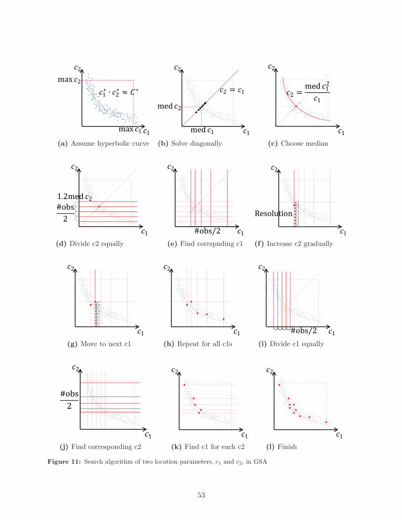
(a) Assume hyperbolic curve (b) Solve diagonally (c) Choose median

(d) Divide c2 equally (e) Find corrspnding c1 (f) Increase c2 gradually

(g) Move to next c1 (h) Repeat for all c1s (i) Divide c1 equally

(j) Find corresponding c2 (k) Find c1 for each c2 (l) Finish

Figure 11: Search algorithm of two location parameters, c1 and c2, in GSA

53

In the step 3, this process is repeated for an odd number of times, and the set of c1

and c2 with the median values is selected (Figure 11c). This median set is more likely to

be located closer to the hyperbolic curve, if the step 2 is repeated for the greater number of

times. However, the efficiency gain from the iterations more than 10 times is small. Then,

we assume the hyperbolic curve as:

c1 � c2 � C� � median�c1� �median�c2� (53)

In the step 4, the tentative maximum of c2 (tmax�c2�) is determined by dividing

median�c1� �median�c2� by the value slightly smaller than median�c1�, say 0.8 �median�c1�.

Similarly, the tentative minimum of c2 (tmin�c2�) is obtained by dividing median�c1� �

median�c2� by the maximum (not tentative) of c2. Formally:

tmax�c2� �median�c1� �median�c2�

0.8 �median�c1�� 1.25 �median�c2� (54)

tmin�c2� �median�c1� �median�c2�

max �c1�(55)

Then, the vertical segment between �0, tmin�c2�� and �0, 1.25 � tmax�c2��, in the vertical axis

is divided into half of the number of observations of equally sized intervals (Figure 11d). In

this example, the number of observation is set at 10 for illustration purpose, but this should

be set at more than 100.

In the step 5, the values of c1 are calculated where the hyperbolic curve estimated

in the step 3 intersects with each of c2 obtained in the step 4 (Figure 11e). The algorithm

determines the values of c1 this way so that PUs are drawn more frequently where the

curvature of the contour is high.

In the step 6, the value of c2 corresponding to the leftmost c1 set at the step 5 is

searched. In doing so, the algorithm first divides the vertical segment between �tmin�c1�, 0�

and �tmin�c1�, tmax�c2�� into a certain number of equidistant intervals.44 In the figure, the

44In the program, this number is specified as resolution.

54

number is set at 9, but this number is usually set at more than 100 because GSA cannot

directly find the set of α and δ that changes the original treatment effect to the target value,

so PUs must be drawn multiple times. Then, the value of c2 is gradually increased up to the

tentative maximum of c2, tmax�c2�, or until the value of c2 is found (Figure 11f).

In the step 7, the algorithm finds the value of c2 in the same way as the step 6 by

fixing c1 at the next value (Figure 11g). In the step 8, the algorithm repeats this process

until c2 is searched for all the fixed values of c1 (Figure 11h).

From the step 9 to the step 11, the procedure from the step 4 to the step 8 is repeated

by switching the roles of c1 and c2 (Figures 11i, 11j, and 11k). We obtain the entire sets of

c1 and c2 by merging the sets of c1 and c2 obtained from the step 4 to the step 8 and those

obtained from the step 9 to the step 11 (Figure 11l).

55