GENERALIZED MAXIMUM FLOW ALGORITHMS

A Dissertation

Presented to the Faculty of the Graduate School

of Cornell University

in Partial Fulfillment of the Requirements for the Degree of

Doctor of Philosophy

by

Kevin Daniel Wayne

January 1999

c© Kevin Daniel Wayne 1999

ALL RIGHTS RESERVED

GENERALIZED MAXIMUM FLOW ALGORITHMS

Kevin Daniel Wayne, Ph.D.

Cornell University 1999

We present several new efficient algorithms for the generalized maximum flow prob-

lem. In the traditional maximum flow problem, there is a capacitated network

and the goal is to send as much of a single commodity as possible between two

distinguished nodes, without exceeding the arc capacity limits. The problem has

hundreds of applications including: shipping freight in a transportation network

and pumping fluid through a hydraulic network.

In traditional networks, there is an implicit assumption that flow is conserved

on every arc. Many practical applications violate this conservation assumption.

Freight may be damaged or spoil in transit; fluid may leak or evaporate. In general-

ized networks, each arc has a positive multiplier associated with it, representing the

fraction of flow that remains when it is sent along that arc. The generalized max-

imum flow problem is identical to the traditional maximum flow problem, except

that it can also model networks which “leak” flow.

Biographical Sketch

Kevin Wayne was born on October 16, 1971 in Philadelphia, Pennsylvania. After

failing a placement exam in seventh grade, Kevin was assigned to a remedial math

class, where he has found memories of modeling conic sections with clay. By the

end of high school, he was taking advanced calculus classes at the University of

Pennsylvania, where he realized there was more to math than playing with clay.

As an undergraduate at Yale University, Kevin stumbled upon a linear program-

ming course, which introduced him to the area of operations research. In 1993, Yale

cut the Department of Operations Research, but not before Kevin was graduated

magna cum laude with a Bachelor of Science.

In Fall 1993, Kevin began the Ph.D. program at Cornell University in the School

of Operations Research and Industrial Engineering. During his first week in Ithaca,

he broke his arm playing football, after crashing into a soccer goal post in the

endzone. This was a harbinger of things to come. While recovering from his first

injury, Kevin quickly rebroke his arm on the basketball court. He also became

passionate about several new classes: skiing, cooking, wine tasting, and network

flows. The first class led to a broken collarbone, the middle two led to many lavish

iii

dinner parties, and the last one ultimately led to his dissertation. While writing

his dissertation, Kevin broke his right hand diving for a softball. At this point he

realized that soccer was his favorite sport, writing a dissertation one-handed is not

much fun, and it’s better to be left-handed.

In the fall, Kevin will be continuing his tour through the Ivy League. He is very

excited to begin teaching at Princeton University in the Department of Computer

Science.

iv

To my loving family.

v

Acknowledgments

First, I would like to express my deepest gratitude to my dissertation supervisor

and mentor Eva Tardos. Without her guidance, encouragement, patience, and

inspiration, the research for this dissertation never would have taken place. I am

also grateful to David Shmoys who acted as a proxy at both my A-exam and B-

exam, and to Jon Kleinberg for serving on my thesis committee.

I am also especially grateful to Professors Jon Lee, Jim Renegar, Sid Resnick,

David Shmoys, Eva Tardos, and Mike Todd. These exceptional faculty have taught

me so much over the years, and have contributed significantly to my intellectual

and professional development.

I am eternally grateful to Mom, Dad, Michele, and Poppop for all of the love

and support they have given me over the years. Without their nourishment, I never

would have had the chance to succeed.

Also, I am grateful for my extended Gaslight family: Agni, Chris, Dawn, Jim,

Jim, John, Mark, Steve, and Vika. I will always have many fond memories of won-

derful food, broken doors, jalapeno-eating squirrels, and dead fish. I am also lucky

to have such wonderful officemates over the past five years. They have provided

vi

lasting friendship, enlightenment, encouragement, and entertainment. Thank you

Agni, Jim, Kathy, Vardges, and Vika. I am also indebted to Nathan and Michael

for their computer wizardry and LATEX 2ε support.

I wish to thank the Defense Advanced Research Projects Agency for supporting

my studies via a National Defense Science and Engineering Graduate Fellowship. I

am also indebted to the Office of Naval Research for supporting my research through

grant AASERT N00014-97-1-0681.

Last, but certainly not least, I would like to thank my orthopedic.

vii

Table of Contents

1 Introduction 11.1 Network Flows . . . . . . . . . . . . . . . . . . . . . . . . . . . . . 11.2 Generalized Maximum Flow Problem . . . . . . . . . . . . . . . . . 21.3 Applications . . . . . . . . . . . . . . . . . . . . . . . . . . . . . . . 31.4 Measuring Efficiency of Algorithms . . . . . . . . . . . . . . . . . . 61.5 Approximation Algorithms . . . . . . . . . . . . . . . . . . . . . . . 71.6 The Combinatorial Approach . . . . . . . . . . . . . . . . . . . . . 81.7 Overview of Dissertation . . . . . . . . . . . . . . . . . . . . . . . . 9

2 Preliminaries 112.1 Basic Definitions . . . . . . . . . . . . . . . . . . . . . . . . . . . . 112.2 Some Traditional Network Flow Problems . . . . . . . . . . . . . . 14

2.2.1 Shortest Path Problem . . . . . . . . . . . . . . . . . . . . . 142.2.2 Minimum Mean Cycle Problem . . . . . . . . . . . . . . . . 152.2.3 Maximum Flow Problem . . . . . . . . . . . . . . . . . . . . 152.2.4 Minimum Cut Problem . . . . . . . . . . . . . . . . . . . . . 172.2.5 Minimum Cost Flow Problem . . . . . . . . . . . . . . . . . 18

2.3 Generalized Maximum Flow Problem . . . . . . . . . . . . . . . . . 202.3.1 Generalized Residual Network . . . . . . . . . . . . . . . . . 222.3.2 Relabeled Network . . . . . . . . . . . . . . . . . . . . . . . 242.3.3 Flow Decomposition . . . . . . . . . . . . . . . . . . . . . . 262.3.4 Optimality Conditions . . . . . . . . . . . . . . . . . . . . . 30

2.4 Canceling All Flow-Generating Cycles . . . . . . . . . . . . . . . . . 322.5 Nearly-Optimal Flows . . . . . . . . . . . . . . . . . . . . . . . . . 33

3 Generalized Maximum Flow Literature 373.1 Combinatorial Methods . . . . . . . . . . . . . . . . . . . . . . . . . 383.2 Linear Programming Methods . . . . . . . . . . . . . . . . . . . . . 413.3 Best Complexity Bounds . . . . . . . . . . . . . . . . . . . . . . . . 42

viii

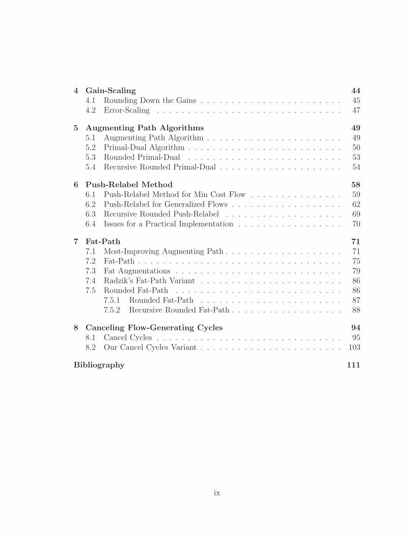
4 Gain-Scaling 444.1 Rounding Down the Gains . . . . . . . . . . . . . . . . . . . . . . . 454.2 Error-Scaling . . . . . . . . . . . . . . . . . . . . . . . . . . . . . . 47

5 Augmenting Path Algorithms 495.1 Augmenting Path Algorithm . . . . . . . . . . . . . . . . . . . . . . 495.2 Primal-Dual Algorithm . . . . . . . . . . . . . . . . . . . . . . . . . 505.3 Rounded Primal-Dual . . . . . . . . . . . . . . . . . . . . . . . . . 535.4 Recursive Rounded Primal-Dual . . . . . . . . . . . . . . . . . . . . 54

6 Push-Relabel Method 586.1 Push-Relabel Method for Min Cost Flow . . . . . . . . . . . . . . . 596.2 Push-Relabel for Generalized Flows . . . . . . . . . . . . . . . . . . 626.3 Recursive Rounded Push-Relabel . . . . . . . . . . . . . . . . . . . 696.4 Issues for a Practical Implementation . . . . . . . . . . . . . . . . . 70

7 Fat-Path 717.1 Most-Improving Augmenting Path . . . . . . . . . . . . . . . . . . . 717.2 Fat-Path . . . . . . . . . . . . . . . . . . . . . . . . . . . . . . . . . 757.3 Fat Augmentations . . . . . . . . . . . . . . . . . . . . . . . . . . . 797.4 Radzik’s Fat-Path Variant . . . . . . . . . . . . . . . . . . . . . . . 867.5 Rounded Fat-Path . . . . . . . . . . . . . . . . . . . . . . . . . . . 86

7.5.1 Rounded Fat-Path . . . . . . . . . . . . . . . . . . . . . . . 877.5.2 Recursive Rounded Fat-Path . . . . . . . . . . . . . . . . . . 88

8 Canceling Flow-Generating Cycles 948.1 Cancel Cycles . . . . . . . . . . . . . . . . . . . . . . . . . . . . . . 958.2 Our Cancel Cycles Variant . . . . . . . . . . . . . . . . . . . . . . . 103

Bibliography 111

ix

List of Figures

1.1 Some Examples of Networks . . . . . . . . . . . . . . . . . . . . . . 21.2 Gain Factors . . . . . . . . . . . . . . . . . . . . . . . . . . . . . . 31.3 Currency Conversion Problem . . . . . . . . . . . . . . . . . . . . . 51.4 Machine Scheduling Problem . . . . . . . . . . . . . . . . . . . . . 6

2.1 Rounding to an Optimal Flow . . . . . . . . . . . . . . . . . . . . 34

4.1 Flow Interpretation . . . . . . . . . . . . . . . . . . . . . . . . . . 46

5.1 Algorithm Primal-Dual . . . . . . . . . . . . . . . . . . . . . . . . 515.2 Algorithm Rounded Primal-Dual . . . . . . . . . . . . . . . . . . . 535.3 Algorithm Recursive Rounded Primal-Dual . . . . . . . . . . . . . 55

6.1 Algorithm Push-Relabel . . . . . . . . . . . . . . . . . . . . . . . . 606.2 Algorithm Rounded Push-Relabel . . . . . . . . . . . . . . . . . . 636.3 Algorithm Recursive Rounded Push-Relabel . . . . . . . . . . . . . 70

7.1 Algorithm Most-Improving Augmenting Path . . . . . . . . . . . . 727.2 Subroutine Finding a Most-Improving Augmenting Path . . . . . . 747.3 Algorithm Fat-Path . . . . . . . . . . . . . . . . . . . . . . . . . . 777.4 Subroutine Fat Augmentations . . . . . . . . . . . . . . . . . . . . 827.5 Algorithm Rounded Fat-Path . . . . . . . . . . . . . . . . . . . . . 877.6 Algorithm Recursive Rounded Fat-Path . . . . . . . . . . . . . . . 90

8.1 Subroutine Cancel Cycles . . . . . . . . . . . . . . . . . . . . . . . 988.2 Subroutine Cancel Cycles2 . . . . . . . . . . . . . . . . . . . . . . 104

x

Chapter 1

Introduction

1.1 Network Flows

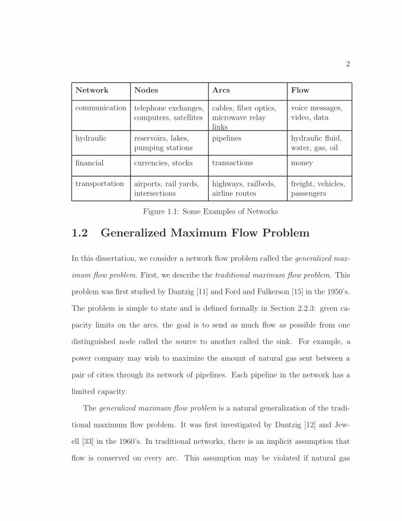
We encounter many different types of networks in our everyday lives, including

electrical, telephone, cable, highway, rail, manufacturing, and, computer networks.

Networks consists of special points called nodes and links connecting pairs of nodes

called arcs. Some examples of networks are listed in Figure 1.1, which is taken

from [1]. In all of these networks, we wish to send some commodity, which we

generically call flow, from one node to another, and do so as efficiently as possi-

ble, subject to certain constraints. Network flow theory is the study of designing

computationally efficient algorithms to solve such problems.

1

2

Network Nodes Arcs Flow

communication telephone exchanges,computers, satellites

cables, fiber optics,microwave relaylinks

voice messages,video, data

hydraulic reservoirs, lakes,pumping stations

pipelines hydraulic fluid,water, gas, oil

financial currencies, stocks transactions money

transportation airports, rail yards,intersections

highways, railbeds,airline routes

freight, vehicles,passengers

Figure 1.1: Some Examples of Networks

1.2 Generalized Maximum Flow Problem

In this dissertation, we consider a network flow problem called the generalized max-

imum flow problem. First, we describe the traditional maximum flow problem. This

problem was first studied by Dantzig [11] and Ford and Fulkerson [15] in the 1950’s.

The problem is simple to state and is defined formally in Section 2.2.3: given ca-

pacity limits on the arcs, the goal is to send as much flow as possible from one

distinguished node called the source to another called the sink. For example, a

power company may wish to maximize the amount of natural gas sent between a

pair of cities through its network of pipelines. Each pipeline in the network has a

limited capacity.

The generalized maximum flow problem is a natural generalization of the tradi-

tional maximum flow problem. It was first investigated by Dantzig [12] and Jew-

ell [33] in the 1960’s. In traditional networks, there is an implicit assumption that

flow is conserved on every arc. This assumption may be violated if natural gas

3

leaks as it is pumped through a pipeline.1 The generalized maximum flow problem

generalizes the traditional maximum flow problem by allowing flow to “leak” as it

is sent through the network. As before, each arc (v, w) has a capacity u(v, w) that

limits the amount of flow sent into that arc. Additionally, each arc (v, w) has a

positive multiplier γ(v, w), called a gain factor, associated with it. For each unit of

flow entering the arc, γ(v, w) units exit. As the example in Figure 1.2 illustrates, if

80 units of flow are sent into an arc (v, w) with gain factor 3/4, then 60 units reach

node w; if these 60 units are then sent through an arc (w, x) with gain factor 1/2,

then 30 units arrive at x.

80 30v w xγ = 3/4 γ = 1/2

Figure 1.2: Gain Factors

1.3 Applications

In traditional networks, there is an implicit assumption that flow is conserved on

every arc. Many practical applications violate this conservation assumption. The

gain factors can represent physical transformations of one commodity into a lesser

or greater amount of the same commodity. Some examples include: spoilage, theft,

evaporation, taxes, seepage, deterioration, interest, or breeding. The gain factors

can also model the transformation of one commodity into a different commodity.1We hope that gas does not actually leak from the pipeline. However, gas in the

pipeline is used to drive the pipeline pumps; effectively, gas leaks as it is shippedthrough the pipeline.

4

Some examples include: converting raw materials into finished goods, currency

conversion, and machine scheduling. We explain the latter two examples next.

Currency conversion

We use the currency conversion problem as an illustrative example of the types

of problems that can be modeled using generalized flows. Later, we will use this

problem to gain intuition. In the currency conversion problem, the goal is to take

advantage of discrepancies in currency conversion rates. Given a certain amount

of one currency, say 1000 U.S. dollars, the goal is to convert it into the maximum

amount of another currency, say French Francs, through a sequence of currency

conversions. We assume that limited amounts of currency can be traded without

affecting the exchange rates.

We model the currency conversion problem as a generalized maximum flow prob-

lem in Figure 1.3. Each node represents a currency, and each arc represents a possi-

ble transaction that converts one currency into another. The source node is dollars

and the sink node is Francs. The gain factor of the arc between two currencies,

say directly from dollars to Francs, is the exchange rate. The capacity of that arc

is the maximum number of the first currency that we can convert into the second

currency. In the example, we can directly convert up to 800 dollars into Francs at

the exchange rate of five Francs per dollar. Note that in this example, it is more

efficient to convert indirectly from dollars to Deutsch Marks to Francs; using this

sequence of conversions we get an effective exchange rate of six Francs per dollar.

5

1,000 $ Y= F

M

exchange rate

capacity limit

γ = 125 γ = 1/21

γ=

9/5u=

400 γ =10/3

γ=

68

γ=

1/70

γ = 5

u = 800

Figure 1.3: Currency Conversion Problem

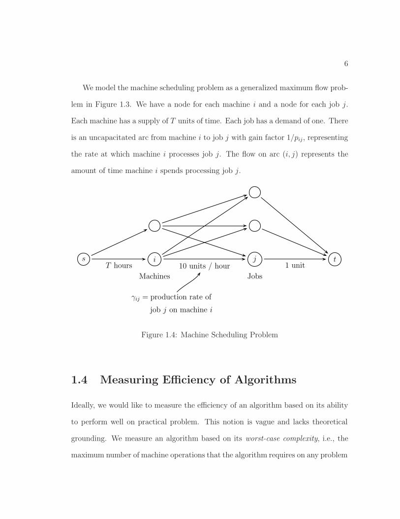
Scheduling unrelated parallel machines

As a second example, we consider the problem of scheduling N jobs to run on M

unrelated machines. The goal is to schedule all of the jobs by a prespecified time

T . Each job must be assigned to exactly one machine. Each machine can process

any of the jobs, but at most one job at a time. Machine i requires a pre-specified

amount of time pij to process job j.

The problem can be formulated as an integer program using assignment variables

to indicate whether job j is processed on machine i. The natural linear program-

ming relaxation is formulated below as a generalized maximum flow problem. The

optimal linear programming solution can be appropriately rounded [41] to produce

an approximately optimal schedule for the original problem.

6

We model the machine scheduling problem as a generalized maximum flow prob-

lem in Figure 1.3. We have a node for each machine i and a node for each job j.

Each machine has a supply of T units of time. Each job has a demand of one. There

is an uncapacitated arc from machine i to job j with gain factor 1/pij, representing

the rate at which machine i processes job j. The flow on arc (i, j) represents the

amount of time machine i spends processing job j.

s i j t

Machines Jobs

γij = production rate of

job j on machine i

10 units / hourT hours 1 unit

Figure 1.4: Machine Scheduling Problem

1.4 Measuring Efficiency of Algorithms

Ideally, we would like to measure the efficiency of an algorithm based on its ability

to perform well on practical problem. This notion is vague and lacks theoretical

grounding. We measure an algorithm based on its worst-case complexity, i.e., the

maximum number of machine operations that the algorithm requires on any problem

7

instance of a given size. For network flow problems, the size depends on the number

of arcs m, the number of nodes n, and the biggest integer B used to represent

capacities, gain factors, and costs. A network flow algorithm is called a polynomial-

time algorithm if its worst-case complexity is bounded by a polynomial function of

m, n, and log2B. We use log2B because it represents the number of bits needed to

store the integer B on a binary computer.

Comparing the performance of algorithms based on their worst-case complexity

has gained widespread acceptance over the past three decades. For a given prob-

lem, the goal is to design a polynomial-time algorithm with the smallest worst-case

complexity. There are many reasons to justify such a goal. First, this provides a

mathematical framework in which we can compare different algorithms. Second,

there is strong computational evidence suggesting a high correlation between an

algorithm’s worst-case complexity and its practical performance. Finally, the study

of polynomial-time algorithms has led to dramatic advances and innovations in the

design of new practical algorithms for a wide variety of problems.

1.5 Approximation Algorithms

For many practical optimization applications, we are often satisfied with solutions

that may not be optimal, but are guaranteed to be “close” to optimal. For example,

if the input data to the problem is only known to a certain level of precision, then

it is often acceptable to only produce a solution of the same level of precision. A

second important reason is that we can often tradeoff solution quality for computa-

8

tional speed; in many applications we can find a provably high quality solution in

substantially less time than it would take to find an optimal solution.

A ξ-approximation algorithm for an optimization problem is a polynomial-time

algorithm that is guaranteed to produce a solution that is within a factor of (1− ξ)

of the optimum. For example, if ξ = 0.01 then a ξ-approximation algorithm for the

maximum flow problem produces a flow that has value at least 99% as large as the

optimum, i.e., it is within 1% of the best possible.

We design both exact and approximation algorithms for the generalized maxi-

mum flow problem. We present a family of ξ-approximation algorithms for every

ξ > 0. This means that we can find nearly optimal solutions to any prescribed level

of precision. For example, when ξ = 0.01 our approximation algorithms are faster

than our exact algorithms by roughly a factor of m, where m is the number of arcs

in the underlying network.

1.6 The Combinatorial Approach

Since the generalized flow problem can be formulated as a linear program, it can be

solved by general purpose linear programming methods including simplex, ellipsoid,

and interior point methods. These continuous optimization methods are grounded

in linear algebra.

The problem can also be solved by combinatorial methods. Combinatorial meth-

ods exploit the discrete structure of the underlying network, often using graph

search, shortest path, maximum flow, and minimum cost flow computations as sub-

9

routines. These methods have led to superior algorithms for many traditional net-

work flow problems including the shortest path, maximum flow, minimum cost flow,

and matching problems. More recently, combinatorial methods have been used to

develop fast approximation algorithms for packing and covering linear programming

problems, including multicommodity flow.

We believe that the best generalized flow algorithms will come from techniques

that exploit the combinatorial structure of the underlying network. This dissertation

takes an important step in this direction.

1.7 Overview of Dissertation

In Chapter 2, we review some basic facts about network flows and generalized flows

that we will use in our algorithms.

In Chapter 3, we review the literature for the generalized maximum flow problem.

In Chapter 4, we introduce a gain-scaling methodology for generalized network

flow problems. Scaling is a powerful technique for deriving polynomial-time algo-

rithms for a wide variety of combinatorial optimization problems. Almost all of the

best traditional network flow algorithms use some form of capacity or cost scaling.

Prior to this thesis, bit-scaling techniques did not appear to apply to generalized

flow problems, in part because there is no integrality theorem. Our gain-scaling

technique provides the basic tools necessary to design several new efficient general-

ized maximum flow algorithms.

10

The primal-dual algorithm is one of the simplest algorithms for the problems,

but requires exponential time. In Chapter 5, we present a polynomial-time variant.

It is the simplest and cleanest polynomial-time approximation algorithm for the

problem.

In Chapter 6, we adapt the push-relabel method of [22] to generalized flows. The

push-relabel method is currently the most practical algorithm for the traditional

maximum flow problem. Our algorithm is the first polynomial-time push-relabel

algorithm for generalized flows. We believe that our push-relabel algorithm will be

quite practical for computing approximate flows.

In Chapter 7, we design a new variant of the Fat-Path capacity-scaling algorithm

of [20]. Our variant matches the best known complexity for the problem, and it is

much simpler than the variant in [49].

In Chapter 8, we discuss a strongly-polynomial variant of a procedure of [20]

which “cancels all flow-generating cycles.” This is used by many of our algorithm

to reroute flow from their current paths to more efficient paths.

Chapter 2

Preliminaries

In this chapter we review several fundamental network flow problems. We formally

define the generalized maximum flow problem and review some basic facts that we

use in the design and analysis of our algorithms.

2.1 Basic Definitions

All of the problems we consider are defined on a directed graph (V,E) where V is

an n-set of nodes and E is an m-set of directed arcs. For notational convenience,

we assume that the graph has no parallel arcs; this allows us to uniquely specify an

arc by its endpoints. Our algorithms easily extend to allow for parallel arcs, and

the complexity bounds we present remain valid. We consider only simple directed

paths and cycles.

11

12

Lengths. The shortest path and minimum mean cycle problems use a length func-

tion l : E → <. The length l(v, w) is the distance from node v to node w. We denote

the length of a cycle (path) Γ by l(Γ) =∑

e∈Γ l(e).

Costs. The minimum cost flow problem uses a cost function c : E → <. The cost

c(v, w) is the unit shipping cost for arc (v, w). We denote the cost of a cycle Γ by

c(Γ) =∑

e∈Γ c(e).

Capacities. The maximum flow, minimum cost flow, and generalized maximum

flow problem use a capacity function u : E → <≥0. The capacity u(v, w) limits the

amount of flow we are permitted to send into arc (v, w).

Symmetry. For the maximum flow and minimum cost flow problems, we assume

the input network is symmetric, i.e., if (v, w) ∈ E then (w, v) ∈ E also. This is with-

out loss of generality, since we could always add the opposite arc and assign it zero

capacity. Without loss of generality, we also assume the costs are antisymmetric,

i.e., c(v, w) = −c(w, v) for every arc (v, w) ∈ E. The reason for these assumption

will become clear in the next paragraph.

Flows. A pseudoflow f : E → < is a function that satisfies the capacity constraints:

∀(v, w) ∈ E : f(v, w) ≤ u(v, w), (2.1)

and the antisymmetry constraints:

∀(v, w) ∈ E : f(v, w) = −f(w, v). (2.2)

13

To gain intuition, it is useful to think of only the nonnegative components of a

pseudoflow. The negative flows are introduced for notational convenience. Note

that we do not need to distinguish between upper and lower capacity limits.

For example, a flow of 17 units sent along arc (v, w) is also viewed as a flow

of −17 units sent along the reverse arc (w, v). The cost of sending one unit of

flow along (v, w) is c(v, w); sending one unit of flow along the opposite arc (w, v)

has cost −c(v, w), and is equivalent to decreasing the flow on arc (v, w) by one

unit. Now, to see how lower bounds are implicitly modeled, suppose arc (w, v)

has zero capacity. This implies that variable f(v, w) is nonnegative: the capacity

constraint for arc (w, v) is f(w, v) ≤ 0, so then the antisymmetry constraint implies

f(v, w) = −f(w, v) ≥ 0.

Residual Networks. With respect to a pseudoflow f in network G, the residual

capacity function uf : E → < is defined by uf(v, w) = u(v, w)−f(v, w). The residual

network is Gf = (V,E, uf). Note that the residual network may include arcs with

zero residual capacity, and still satisfies the symmetry assumption.

For example, if u(v, w) = 20, u(w, v) = 0, and f(v, w) = −f(w, v) = 17, then

arc (v, w) has 20 – (–17) = 3 units of residual capacity, and arc (w, v) has 0 – (–17)

= 17 units of residual capacity.

We define Ef = {(v, w) ∈ E : uf(v, w) > 0} to be the set of all arcs in Gf with

positive residual capacity. A residual arc is an arc with positive capacity. A residual

path (cycle) is a path (cycle) consisting entirely of residual arcs.

14

2.2 Some Traditional Network Flow Problems

In this section we formally define the shortest path, minimum mean cycle, maximum

flow, minimum cut, and minimum cost flow problems. We also state the best

known complexity bounds. We will use these as subroutines in our generalized flow

algorithms.

2.2.1 Shortest Path Problem

In the shortest path problem, the goal is to find a simple path between two nodes,

so as to minimize the total length. An instance of the shortest path problem is a

network G = (V,E, s, l), where s ∈ V is a distinguished node called the source, and

l is a length function. The problem is NP-hard if negative length cycles are allowed.

In networks with no negative length cycles, there are a number of polynomial-

time algorithms for the problem, e.g. Bellman-Ford. There are faster specialized

algorithms for networks with nonnegative arc lengths, e.g., Dijkstra.

We let SP(m,n) denote the complexity of solving a shortest path problem in a

network with m arcs, and n nodes, and nonnegative lengths. Currently, the best

known bound for SP(m,n) is O(m + n log n) due to [17]. Recently, Thorup [53]

developed a linear time algorithm for the problem; his algorithm performs bit ma-

nipulations on the input numbers. We let SP(m,n,C) be the complexity assuming

the lengths are integers between 0 and C. Currently, the best known bounds for

SP(m,n, C) are O(m log logC) and O(m + n√

logC) due to [34], and [2], respec-

tively.

15

If negative length arcs are allowed (but no negative length cycles), then the best

strongly polynomial complexity bound is O(mn) due to Bellman [5] and Ford [16].

The best weakly polynomial bound is O(m√n logC) due to [].

2.2.2 Minimum Mean Cycle Problem

In the minimum mean cycle problem, the goal is to find a cycle whose ratio of

length to number of arcs is minimum. That is, we want to find a cycle Γ that

minimizes l(Γ)/|Γ|. An instance of the minimum mean cost cycle problem is a

network G = (V,E, l), where l is a length function. Although it is NP-hard to

find a cycle of minimum length, it is possible to find a minimum mean cycle in

polynomial-time. Virtually all known algorithms are based upon a shortest path

computation in a network where negative length arcs are allowed.

We let MMC(m,n) denote the complexity of finding a minimum mean cost cycle

in a network with m arcs, n nodes, and arbitrary costs. Currently, the best known

bound for MMC(m,n) is O(mn) due to Karp [38]. We let MMC(m,n,C) denote

the complexity assuming the lengths are integers between −C and C. Currently,

the best known bound for MMC(m,n, C) is O(m√n log(nC)) due to Orlin and

Ahuja [46].

2.2.3 Maximum Flow Problem

In the maximum flow problem, the goal is to send as much flow as possible between

two nodes, subject to arc capacity limits. An instance of the maximum flow problem

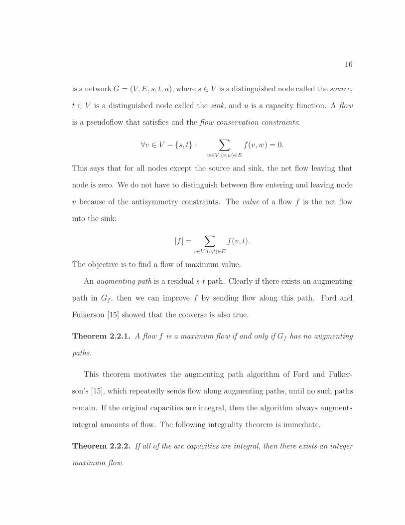
16

is a network G = (V,E, s, t, u), where s ∈ V is a distinguished node called the source,

t ∈ V is a distinguished node called the sink, and u is a capacity function. A flow

is a pseudoflow that satisfies and the flow conservation constraints:

∀v ∈ V − {s, t} :∑

w∈V :(v,w)∈E

f(v, w) = 0.

This says that for all nodes except the source and sink, the net flow leaving that

node is zero. We do not have to distinguish between flow entering and leaving node

v because of the antisymmetry constraints. The value of a flow f is the net flow

into the sink:

|f | =∑

v∈V :(v,t)∈E

f(v, t).

The objective is to find a flow of maximum value.

An augmenting path is a residual s-t path. Clearly if there exists an augmenting

path in Gf , then we can improve f by sending flow along this path. Ford and

Fulkerson [15] showed that the converse is also true.

Theorem 2.2.1. A flow f is a maximum flow if and only if Gf has no augmenting

paths.

This theorem motivates the augmenting path algorithm of Ford and Fulker-

son’s [15], which repeatedly sends flow along augmenting paths, until no such paths

remain. If the original capacities are integral, then the algorithm always augments

integral amounts of flow. The following integrality theorem is immediate.

Theorem 2.2.2. If all of the arc capacities are integral, then there exists an integer

maximum flow.

17

We let MF(m,n) denote the worst-case complexity of finding a maximum flow

in a network with m arcs, n nodes, and arbitrary positive capacities. Currently,

the best known bounds on MF(m,n) are O(mn log(n2/m)), O(mn logm/n logn n),

and O(mn logm/n n+ n2 log2+ε n) for any constant ε > 0, due to [22], [39], and [47],

respectively. We let MF(m,n, U) denote the complexity assuming the capacities are

integers between 0 and U . Currently, the best known bounds for MF(m,n, U) are

O(mn log(n√

logU/(m + 2)) and O(min{n2/3,√m}m log(n2/m) logU) due to [3],

and [21], respectively.

2.2.4 Minimum Cut Problem

The s-t minimum cut problem is intimately related to the maximum flow problem.

The input is the same as for the maximum flow problem. The goal is to find a

partition of the nodes that separates the source and sink, so that the total capacity

of arcs going from the source side to the sink side is minimum. Formally, we define

an s-t cut [S, T ] to be a partition of the nodes V = S ∪ T so that s ∈ S and t ∈ T .

The capacity of a cut is defined to be the sum of the capacities of “forward” arcs in

the cut:

u[S, T ] =∑

v∈S,w∈Tu(v, w). (cut capacity)

The goal is to find an s-t cut of minimum capacity.

It is easy to see that the value of any flow is less than or equal to the capacity of

any s-t cut. Any flow sent from s to t must pass through every s-t cut, since the cut

disconnects s from t. Since flow is conserved, the value of the flow is limited by the

18

capacity of the cut. A cornerstone result of network flows is the much celebrated

max-flow min-cut theorem of Ford and Fulkerson [15]. It captures the fundamental

duality between the maximum flow and minimum cut problems.

Theorem 2.2.3. The maximum value of any flow from the source s to the sink t

in a capacitated network is equal to the minimum capacity among all s-t cuts.

Proof. By our previous observation, it is sufficient to show that the capacity of some

s-t cut equals the value of some flow. Let f be a maximum flow. Choose S to be

the set of nodes reachable from the source using only residual arcs in Gf , and let

T = V \ S. We show that [S, T ] is an s-t cut of capacity |f |. Clearly s ∈ S and

t ∈ T . By the definition of S, flow f saturates every “forward” arc in the cut,

and does not send flow along any “backward” arcs in the cut. Thus, the net flow

crossing the cut is u[S, T ]. By flow conservation, the net flow sent across any s-t

cut is equal to the value of the flow; thus u[S, T ] = |f |.

2.2.5 Minimum Cost Flow Problem

In the minimum cost flow problem, the goal is to send flow from supply nodes

to demand nodes as cheaply as possibly, subject to arc capacity constraints. An

instance of the minimum cost flow problem is a network G = (V,E, b, u, c), where

b : V → < is a supply function, u is a capacity function, and c is a cost function. We

say node v ∈ V has supply if b(v) > 0 and demand if b(v) < 0. We assume that the

total supply equals the total demand, i.e.∑

v∈V b(v) = 0; otherwise the problem is

19

infeasible. A flow is a pseudoflow that satisfies the mass balance constraints:

∀v ∈ V :∑

w∈V :(v,w)∈E

f(v, w) = b(v).

Let f be a flow. If there exists a negative cost residual cycle in Gf , then we can

improve f by sending flow around the cycle. Busacker and Saaty [8] showed that

the converse is also true.

Theorem 2.2.4. A flow f is a minimum cost flow if and only if Gf contains no

negative cost residual cycles.

Now, we describe an alternate set of optimality conditions. We refer to a function

π : V → < as a set of node potentials. The reduced cost of an arc (v, w) ∈ E with

respect to node potentials π is defined to be:

cπ(v, w) = c(v, w)− π(v) + π(w). (reduced cost)

Intuitively, we can view −π(v) as the market price for buying or selling one unit

of flow at node v. The reduced cost is then the cost of buying one unit at node v,

shipping it to node w, and selling it at node w.

The complementary slackness optimality conditions express the negative cost

cycle optimality conditions in terms of reduced costs. It says the a flow is optimal

if and only if there are prices π so that there is no incentive to buy flow, ship it,

and then sell it.

Theorem 2.2.5. A flow f is a minimum cost flow if and only if there exists a set

of node potentials π such that:

∀(v, w) ∈ Ef : cπ(v, w) ≥ 0. (2.3)

20

Proof. Let f be a flow and let π be potentials that satisfy (2.3). All residual arcs

have nonnegative cost. Then, there are no negative cost residual cycles in Gf . The

cost of a cycle is equal to the reduced cost of the cycle; hence flow f is optimal by

Theorem 2.2.4.

Now suppose f is a minimum cost flow. Then by Theorem 2.2.4, there are no

negative cost residual cycles in Gf . Let π(v) be the shortest path from node v to

some designated node t in the graph (V,Eg) using lengths c. The shortest path

distances are well-defined and the shortest path optimality conditions imply that π

satisfies (2.3).

2.3 Generalized Maximum Flow Problem

In this section, we formally define the generalized maximum flow problem. We

define the residual and the relabeled networks. These networks will be useful in

the design of our algorithms. We also characterize the optimality conditions for the

problem.

Gains. The generalized maximum flow problem uses a gain function γ : E → <>0.

For each unit of flow that enters arc (v, w) at node v, only γ(v, w) units arrive at node

w. A lossy arc is an arc with gain factor at most one. Without loss of generality,

we assume that the gain function is symmetric, i.e., γ(v, w) = 1/γ(w, v). If this

assumption is not satisfied, we can add the symmetric arc and give it a capacity of

zero. We will see that this is a natural assumption in the next paragraph.

21

Generalized pseudoflow. A generalized pseudoflow is a function g : E → <

that satisfies the capacity constraints (2.1) and the and generalized antisymmetry

constraints:

∀(v, w) ∈ E : g(v, w) = −γ(w, v)g(w, v).

To gain intuition, it is useful to think of only the positive components of a pseud-

oflow. As before, the negative flows are introduced for notational convenience and

we do not need to distinguish between upper and lower capacity limits.

If we send 200 units of flow into an arc (v, w) with a gain factor of 1/5, then

this would produce 40 units of flow at node w. This is also viewed as sending –40

units of flow along arc (w, v), which has a gain factor of 5.

The problem. In the generalized maximum flow problem, the goal is to send as

much flow as possible between two nodes, subject to arc capacity constraints. Also,

flow “leaks” as it is sent through the network.

Since some of our algorithms are recursive, it is convenient to solve a seem-

ingly more general version of the problem which allows multiple sources. An in-

stance of the generalized maximum flow problem is a generalized network G =

(V,E, t, u, γ, e), where t ∈ V is a distinguished node called the sink, u is a capacity

function, γ is a gain function, and e : V → <≥0 is an initial excess function.

The residual excess of a generalized pseudoflow g at node v is defined by:

eg(v) = e(v)−∑

(v,w)∈E

g(v, w).

22

It is the initial excess minus the net flow leaving v. If eg(v) is positive (negative) we

say that g has residual excess (deficit) at node v. A generalized flow is a generalized

pseudoflow that has no residual deficits, but it is allowed to have residual excesses.

A proper generalized flow is a flow which does not generate any additional residual

excesses, except possibly at the sink. We will show in Corollary 2.3.6 that a flow

can be efficiently converted into a proper flow that generates the same amount of

residual excess at the sink. For a flow g we denote its value |g| = eg(t) to be the

residual excess at the sink.

Let OPT(G) denote the maximum possible value of any flow in network G. A

flow g in networkG is optimal if |g| = OPT(G) and ξ-optimal if |g| ≥ (1−ξ) OPT(G).

The generalized maximum flow problem is to find an optimal flow. The approximate

generalized maximum flow problem is to find a ξ-optimal flow.

Size of numbers. We assume the capacities and initial excesses are given as

integers between 1 and B, and the gains are given as ratios of integers which are

between 1 and B. We assume B ≥ 2, since otherwise the problem reduces to a

traditional minimum cost flow problem. To simplify the running times we use O(f)

to denote f logO(1) m.

2.3.1 Generalized Residual Network

We extend the definition of a residual network to generalized flows by appropri-

ately accounting for the gain factors. Let g be a generalized flow in network G =

23

(V,E, s, u, γ, e). With respect to the flow g, the residual capacity function is defined

by ug(v, w) = u(v, w)− g(v, w). The residual network is Gg = (V,E, s, ug, γ, eg).

To gain intuition, we consider an example from the currency conversion problem

that was described in Section 1.3. Let node v represent U.S. dollars and let node w

represent French Francs. Suppose that we can convert up to 30 dollars into Francs

at the exchange rate of 5 Francs per dollar, i.e., u(v, w) = 30, u(w, v) = 0, and

γ(v, w) = 5. If we convert g(v, w) = 20 dollars, then we obtain 100 Francs. We can

still convert up to ug(v, w) = 10 dollars into Francs at the same exchange rate. We

can also unconvert any or all of the ug(w, v) = 0 – g(w, v) = g(v, w)/γ(v, w) = 100

Francs back into dollars at the symmetric exchange rate of γ(w, v) = 0.2 dollars per

Franc. Note that in general, the exchange rates are not symmetric, but here we are

undoing a previous transaction, not creating a new one.

The following lemma is straightforward. It says that solving the problem in the

residual network is equivalent to solving it in the original network.

Lemma 2.3.1. Let g be a generalized flow in network G and let g′ be a generalized

flow in the residual network Gg. Then OPT(G) = |g| + OPT(Gg). Generalized

flow g′ is a generalized maximum flow in Gg if and only if g + g′ is a generalized

maximum flow in G.

As before, we define Eg = {(v, w) ∈ E : ug(v, w) > 0} to be the set of residual

arcs in Gg. We also define residual arcs, paths, and cycles as before. A lossy network

is a network in which each residual arc is lossy, i.e., no residual arc has gain factor

exceeding one.

24

2.3.2 Relabeled Network

With respect to generalized network G = (V,E, t, u, γ, e), a labeling function is a

function µ : V → <>0 ∪ {∞} such that µ(t) = 1. We note that the node labels are

the inverses of the linear programming dual variables, corresponding to the primal

problem with decision variables {g(v, w) : (v, w) ∈ E}. This idea of relabeling was

originally introduced by Glover and Klingman [19]. Intuitively, node label µ(v)

changes the local units in which flow is measured at node v; it is the number of

old units per new unit. For example, in the currency conversion problem, if we

change the basic unit of currency at node v from U.S. dollars to pennies, then

µ(v) = 1/100. To create an equivalent problem using the new units, we must

appropriately normalize the capacity limits, gain factors, and initial excesses.

Continuing with the currency conversion example, suppose that we start with

1,700 dollars at node v, then in the new problem we start with 1,700,000 pennies.

Similarly, if we could convert up to 800 dollars into Francs at the exchange rate of

5 Francs per dollar, then now we can convert up to 80,000 pennies into Francs at

the exchange rate of 5/100 Francs per penny.

Thus, it is natural to define for each (v, w) ∈ E, the relabeled capacities, relabeled

gains, and relabeled initial excesses by:

uµ(v, w) = u(v, w)/µ(v) (relabeled capacity)

γµ(v, w) = γ(v, w)µ(v)/µ(w) (relabeled gain)

eµ(v) = e(v)/µ(v). (relabeled initial excess)

25

The relabeled network is denoted by Gµ = (V,E, t, uµ, γµ, eµ). The following lemma

is straightforward. It says that the relabeled network is an equivalent instance of

the generalized maximum flow problem.

Lemma 2.3.2. For any labeling function µ, g is a generalized flow in network G

if and only if gµ(v, w) = g(v, w)/µ(v) is a generalized flow of the same value |g| in

network Gµ.

By relabeling the residual network, we can create new equivalent instances of

the generalized maximum flow problem. With respect to a flow g and labels µ, we

define the relabeled residual capacities and relabeled residual excesses by:

ug,µ(v, w) = ug(v)/µ(v) (relabeled residual capacity)

eg,µ(v) = eg(v)/µ(v). (relabeled residual excess)

The relabeled residual network is denoted by Gg,µ = (V,E, t, ug,µ, γµ, eg,µ).

Canonical Labels. We define the canonical label of a node v in network G to be

the inverse of the highest gain residual path from v to the sink. If no such path

exists, its label is∞. If G has no residual flow-generating cycles, then the canonical

labels can be determined using a single Bellman-Ford shortest path computation

with lengths l = − log γ. If G is a lossy network, then a Dijkstra shortest path

computation suffices.

26

2.3.3 Flow Decomposition

A traditional pseudoflow can be decomposed into a collection of at mostm paths and

cycles. In this section, we show how a generalized pseudoflow g can be decomposed

into a small collection of “elementary” generalized pseudoflows that conform to g.

By conform, we mean that the elementary pseudoflows can only be positive on arcs

on which g is positive. In addition, the elementary pseudoflow can only generate

excess (deficit) at a node for which g generates excess (deficit).

This decomposition is useful to characterize the optimality conditions for the

generalized maximum flow problem. It can also simplify a generalized flow by

eliminating flow which does not reach the sink; this enables us to convert a flow

into a proper flow of the same value. Also, it leads to an alternate “path-based

formulation” of the problem.

We denote the gain of a cycle (path) Γ by γ(Γ) =∏

e∈Γ γ(e). A unit-gain cycle

has gain equal to one. A flow-generating (flow-absorbing) cycle is a cycle with gain

more (less) than one. We remark if we use the logarithmic cost function c = − log γ,

then flow-generating cycles are in one-to-one correspondence with negative cost

cycles.

There are five types of elementary generalized pseudoflows:

• Type I (path): It is positive only on the arcs of a path. It only creates deficit

at the first node of the path and excess at the last node.

• Type II (unit-gain cycle): It is positive only on the arcs of a unit gain cycle.

It does not create excess or deficit.

27

• Type III (cycle-path): It is positive only on the arcs of a flow-generating cycle

and a (possibly trivial) path connecting the cycle to a node. It only creates

excess at the endpoint of the path.

• Type IV (path-cycle): It is positive only on the arcs of a flow-absorbing cycle

and a (possibly trivial) path from a node to the cycle. It only creates deficit

at the endpoint of the path.

• Type V (bicycle): It is positive only on the arcs of a flow-generating cycle, a

flow-absorbing cycle and a (possibly trivial) path connecting the two cycles.

It does not create excess or deficit.

The following theorem is due to Gondran and Minoux [29]. We repeat the proof

from [20].

Theorem 2.3.3. For every pseudoflow g, there exists a collection of k ≤ m ele-

mentary pseudoflows g1, . . . , gk that conform to g such that g(v, w) =∑

i gi(v, w).

Such a decomposition can be found in O(mn) time.

Proof. We prove by induction on the number of arcs with positive flow. Let G′ be

the subgraph of G consisting of arcs with positive flow.

If G′ is acyclic then we can trace the flow from any deficit node to some excess

node along a path, and subtract flow on the path until one arc on the path has zero

flow. The subtracted flow is of Type I, and the theorem follows by induction.

Otherwise, let Γ be a cycle in G′. If γ(Γ) = 1, then we can subtract flow around

the cycle until one arc on the cycle has zero flow. The subtracted flow is of Type

II, and the theorem follows by induction.

28

Otherwise, suppose Γ is a flow-generating cycle (the case when Γ is a flow-

absorbing cycle is similar). We subtract flow around the cycle until one arc on the

cycle has zero flow, and let h denote the flow removed. This reduces the excess

at one of the nodes, say v, possibly to a negative value. If node v no deficit after

reducing flow around the cycle, then the subtracted flow is of Type III (with a

trivial path), and the theorem follows by induction. Otherwise we decompose g–h

inductively. Now, since v has deficit, the decomposition of g–h includes components

of Type I or IV that are responsible for creating all of the deficit at node v. Each

of these components, together with an appropriate fraction of h, corresponds to a

component of Type III or V in the decomposition of g. If node v originally had

positive excess in G, then there will be some fraction of h left over; this is a Type

III pseudoflow (with a trivial path).

The above procedure strictly decreases the number of arcs with positive flow in

amortized O(n) time.

An augmenting path is a residual path from a node with excess to the sink.

It corresponds to a Type I pseudoflow whose first node has excess in the original

network, and whose last node is the sink.

Corollary 2.3.4. Let G be a lossy network. Then, there exists a generalized max-

imum flow that is positive on at most m augmenting paths.

Proof. Let g∗ be a generalized maximum flow. We decompose it according to The-

orem 2.3.3. Note that there are no Type III or V components in the decomposition,

since G is a lossy network. We remove all components that do not generate excess

29

at the sink, and denote the resulting flow by g. This removes all Type II and IV

components, and also some Type I components. The only components that remain

are Type I components that generate excess at the sink. These correspond to aug-

menting paths. It follows that g is also optimal and can be decomposed into at

most m augmenting paths.

A generalized augmenting path (GAP) is a residual flow-generating cycle, to-

gether with a (possibly trivial) residual path from a node on this cycle to the sink.

It corresponds to a Type III pseudoflow whose path ends at the sink.

Corollary 2.3.5. Let G be a generalized network. Then, there exists a generalized

maximum flow that is positive on at most m augmenting paths or GAPs.

Proof. Let g∗ be a generalized maximum flow. We decompose it according to The-

orem 2.3.3. We remove all components that do not generate excess at the sink, and

denote the resulting flow by g. As above, the only Type I components that can

generate excess at the sink correspond to augmenting paths. The only Type III

components that generate excess at the sink correspond to GAPs. The corollary

immediately follows.

Recall, a generalized flow is allowed to generate excesses, but no deficits. A

proper flow does not generate any additional excesses, except possibly at the sink.

Corollary 2.3.6. Let g be a flow in network G. Then in O(mn) time we can find

a proper flow g′ in G such that |g′| ≥ |g|.

30

Proof. Let g be a flow. We decompose it according to Theorem 2.3.3. As above, the

only components that generate excess at the sink correspond to augmenting paths

and GAPs. Moreover, these components do not generate excess at any other node.

Let g′ be the flow induced by only these useful components. Now g′ is a proper flow

and |g′| ≥ |g|.

Path-Based Formulation. Now, we consider an alternate path-based formula-

tion for the generalized maximum flow problem in lossy networks. In this formula-

tion, we have a nonnegative variable x(P ) for each augmenting path P , representing

the amount of flow sent along P . We also include a capacity constraint for each arc.

The objective is to maximize the net flow into the sink:∑

P augmenting path γ(P )x(P ).

Corollary 2.3.4 implies that the path formulation is equivalent to the “arc-based”

formulation considered in Section 2.3. We note that the path-based formulation

may have exponentially many variables.

2.3.4 Optimality Conditions

Let g be a generalized flow in network G. If Gg has an augmenting path, then we

can improve g by augmenting flow along such a path. By augmenting flow, we mean

increasing the flow of forward arcs along the residual path (and decreasing flow on

the reverse arcs to maintain generalized antisymmetry), while conserving flow at

intermediate nodes of the path. If one unit of flow is sent from node v to the sink

along augmenting path P , then γ(P ) units arrive at t.

31

If Gg has a GAP, then we can improve g by augmenting flow along such a GAP.

If one unit of flow is sent from a node v around a residual flow-generating cycle,

then more than one unit arrives back at v. By sending flow around such a cycle, we

can increase the residual excess at any node of the cycle, while conserving flow at

all other nodes. This excess can subsequently be sent along a residual path to the

sink, which increases the excess at t.

The following theorem of Onaga [44] says that these are the only two ways to

improve the current flow g. It generalizes Theorem 2.2.1.

Theorem 2.3.7. A generalized flow g is a generalized maximum flow if and only

if Gg has no augmenting paths or GAPs.

Proof. Clearly if a generalized flow g has an augmenting path or GAP in Gg then

it is not optimal.

Now, suppose g has no augmenting paths or GAPs in Gg. Let g∗ be a generalized

maximum flow. Decompose g∗ – g according to Theorem 2.3.3. Since g has no

augmenting paths or GAPs, there are none in the decomposition either. These are

the only two elementary pseudoflows that can generate excess at the sink. Hence g

is optimal.

The following theorem expresses the optimality conditions in terms of node

labels.

Theorem 2.3.8. A generalized flow g is a generalized maximum flow if and only

if there exists labels µ such that:

∀ (v, w) ∈ Gg : γµ(v, w) ≤ 1 (2.4)

32

∀ v that cannot reach t in Gg : µ(v) =∞. (2.5)

Proof. The proof is immediate from linear programming duality; the node labels

are the inverses of the dual variables. We now give a direct combinatorial proof.

Suppose g is a generalized maximum flow. Let µ be the canonical labels in

Gg. Let T be the set of nodes that can reach the sink using residual arcs in Gg.

Since Gg has no GAPs, T has no flow-generating cycles. Consequently, the labels

are well-defined and can be computed efficiently using a Bellman Ford shortest

path computation with lengths l = − log γ. As a result, the labels satisfy µ(w) ≥

γ(v, w)µ(v) for residual arcs in the subgraph of Gg induced by nodeset T .

By definition of the canonical labels, all labels are positive, µ(t) = 1, and µ(v) =

∞ for all nodes v ∈ V \ T . Thus µ satisfies (2.4) and (2.5).

Now, suppose generalized flow g and labels µ satisfy (2.4) and (2.5). Then,

there can be no residual paths from excess nodes to the sink. Also the gain of

a cycle is equal to the relabeled gain of a cycle; thus, there are no residual flow-

generating cycles involving nodes that can reach the sink. Thus, by Theorem 2.3.7,

g is optimal.

2.4 Canceling All Flow-Generating Cycles

In this section we briefly review a procedure for “canceling all flow-generating cy-

cles.” It is described in detail in Chapter 8. Many generalized flow computations

can be performed much more efficiently in networks without residual flow-generating

cycles. To overcome this obstacle, we send flow around a residual flow-generating

33

cycle until one (or more) arcs become saturated. In the process additional excesses,

but no deficits, may be created. This operation is called canceling a flow-generating

cycle. The goal is to repeatedly cancel residual flow-generating cycles, until no such

cycles remain. Goldberg, Plotkin, and Tardos [20] proposed an efficient method

that is based on the Cancel-and-Tighten algorithm of Goldberg and Tarjan [23].

Their algorithm requires O(mnmin{m,n logB}) time.

2.5 Nearly-Optimal Flows

The optimality conditions for the generalized maximum flow problem are charac-

terized by Theorem 2.3.7 and Theorem 2.3.8. We now give conditions under which

a flow is essentially optimal. Given a generalized flow g in network G, the excess

discrepancy is the difference between the value of the optimal flow and the current

flow, i.e., OPT(G) − |g|. The following lemma from [20] says that if the excess

discrepancy is very small and there are no residual flow-generating cycles, then the

flow can be “rounded” to an optimal solution. We give a modification of their proof.

Lemma 2.5.1. Let g be a flow in network G such that OPT(G)− |g| < B−m and

Gg has no residual flow-generating cycles. Then, we can find an optimal flow in

O(MF(m,n)) time.

Proof. Without loss of generality, we assume that there is a residual path in Gg

from every node to the sink; otherwise we could delete such useless nodes. Let µ

be the canonical labels in Gg. Since Gg has no residual flow-generating cycles, the

labels are well defined. We find a flow g∗ that satisfies the complementary slackness

34

conditions (2.4) with µ, and, among all such flows, maximizes the excess at the sink.

We will argue that g∗ is optimal (and hence µ is dual optimal). The procedure for

determining g∗ is given in Figure 2.1 and is described below.

Input: network G, flow g such that Gg has no residual flow-generating cycles and

OPT(G)− |g| < B−m

Output: maximum flow g∗

µ← canonical labels in Gg

h← flow that saturates all arcs with relabeled gain above one, and sends zero

h← flow on all arcs with relabeled gain equal to one

G′g,µ ← subgraph of Gg,µ induced by gain one arcs

Consider excess nodes as sources with capacity eg,µ(v) and deficit nodes as sinks

h← with demand |eg,µ(v)|. Compute flow f ′ in G′g,µ that satisfies all demand

h← and maximizes net flow into t

g∗(v, w)← h(v, w) + µ(v)f ′(v, w)

Figure 2.1: Rounding to an Optimal Flow

Let h denote the pseudoflow that satisfies (2.4) and sends zero flow on every arc

with unit relabeled gain. The relabeled node excess of pseudoflow h at node v is:

eh,µ(v) = eµ(v)−∑

w:(v,w)∈E

hµ(v, w) = eµ(v)−∑

w:(v,w)∈E,γµ(v,w)>1

uµ(v, w).

The original capacities and excesses are integral. The canonical labels are integral

multiples of L−1, where L is the least common denominator of the gains of paths

in G. Thus, the relabeled excesses and capacities are also integral multiples of L−1.

In particular, |hµ| = eh,µ(t) is an integral multiple of L−1.

35

The procedure finds a generalized flow g∗ that maximizes the excess at the sink

among all flows that satisfy (2.4). To find such a flow, let G′g,µ denote the subgraph

of Gg,µ induced by gain one arcs. We view excess nodes in Gg,µ as sources with

capacity eg,µ(v) and deficit nodes as sink nodes with demand |eg,µ(v)|. Let fµ = f ′

be a traditional flow in G′g,µ that satisfies all of the demand, and maximizes the net

flow into the sink. Note that such a flow is guaranteed to exists, since the restriction

of gµ to gain one arcs in Gg,µ is such a flow. We can compute fµ using a traditional

maximum flow computation. By the integrality theorem for the maximum flow

problem, since all of the demands and capacities are integral multiples of L−1,

then so is the value of the maximum flow |fµ|. Let g∗ = h + f , where f is the

“unrelabeled” version of fµ. Now |g∗| ≥ |g| Thus OPT(G) − |g∗| < B−m. Since

|g∗| = |h| + |f | = |hµ| + |fµ| and OPT(G) are both integral multiples of L−1, and

L ≤ Bm, it follows that g∗ is optimal.

The next lemma indicates that if a generalized flow is ξ-optimal for sufficiently

small ξ, then it is essentially optimal. It is used to provide termination of our exact

algorithms.

Lemma 2.5.2. Let g be a B−3m-optimal flow in network G. Then we can compute

an optimal flow in G in O(mnmin{m,n logB}) time.

Proof. Let g be a B−3m-optimal flow. Then the excess discrepancy of g is

OPT(G)− |g| ≤ B−3m OPT(G) ≤ B−m.

36

The last inequality follows since each arc entering the sink has capacity and gain

each at most B; therefore OPT(G) ≤ mB2 ≤ Bm+1. The lemma then follows from

Lemma 2.5.1 provided Gg has no residual flow-generating cycles.

If there are residual flow-generating cycles in Gg, then we can cancel them in

the stated time bound, as described in Section 2.4. Canceling flow-generating cycles

can only create additional excesses. Thus, the resulting flow is also B−3m-optimal,

and the previous argument applies.

Chapter 3

Generalized Maximum Flow

Literature

In this chapter we review the generalized maximum flow literature. Since the gen-

eralized flow problem is a special case of linear programming, it can be solved by

general purpose linear programming techniques. The problem can also be solved

by combinatorial methods, which have led to superior algorithm for many tradi-

tional network flow problems. In the 1960’s Jewell [33] and Onaga [44] proposed

exponential-time augmenting path algorithm for the generalized maximum flow

problem. It wasn’t until the late 1980’s that Goldberg, Plotkin and Tardos [20]

designed the first polynomial-time combinatorial algorithms for the generalized max-

imum flow problem.

37

38

3.1 Combinatorial Methods

Exact algorithms. The first combinatorial algorithms for the generalized maxi-

mum flow problem were exponential-time augmenting path algorithms proposed by

Jewell [33] and Onaga [44]. The generalized maximum flow problem is closely re-

lated to the traditional minimum cost flow problem. Truemper [55] observed that by

using the cost function c = − log γ, many of the early generalized maximum flow al-

gorithms were, in fact, analogs of pseudo-polynomial minimum cost flow algorithms.

Jewell’s [33] generalized maximum flow algorithm is an analog of Klein’s [40] cycle-

canceling algorithm for the minimum cost flow problem. Similarly, Onaga’s [44]

algorithm is analogous to the successive shortest path algorithm developed inde-

pendently by Busacker and Gowen [7], Iri [30], and Jewell [32]. Truemper’s [54]

algorithm is an analog of Ford and Fulkerson’s [16] primal-dual algorithm. Jarvis

and Jezior’s [31] algorithm is an analog of Fulkerson’s [18] out-of-kilter algorithm.

Goldberg, Plotkin, and Tardos [20] designed the first two polynomial-time com-

binatorial algorithms for the generalized maximum flow problem: Fat-Path and

MCF. They also developed much of the machinery used in subsequent generalized

flow algorithms. The Fat-Path algorithm maintains a generalized flow and uses

capacity-scaling. The main idea is to repeatedly send along “fat-paths”, i.e., paths

that have enough capacity to generate large amounts of excess at the sink. Peri-

odically, flow is rerouted to more efficient paths by “cancelling all flow-generating

cycles.” The algorithm requires O(m2n2 log2B) time. It is described in detail in

Chapter 7.

39

Algorithm MCF maintains a pseudoflow with no excess nodes, except the source.

It repeatedly performs a traditional minimum cost flow computation with cost func-

tion c = − log γ. It interprets the result as an augmentation from the source to

deficit nodes in the generalized network. It requires O(m2n2 logB) time.

Radzik [49] modified the Fat-Path algorithm and improved the complexity to

O(m3 logB+m2n logB log logB). The bottleneck computation in the original Fat-

Path algorithm is cancelling flow-generating cycles. Radzik reduces this bottleneck

by only canceling flow-generating cycles that have sufficiently large gain. Since

there are still residual flow-generating cycles, finding fat-paths becomes much more

complicated.

Goldfarb and Jin [26] designed an algorithm based on the MCF algorithm. It

matches the complexity of the original MCF algorithm, without using the dynamic

tree data structure. Instead of using a traditional minimum cost flow computation

at each iteration, they augment flow along highest-gain paths. They introduced

the concept of “arc deficits” to ensure that most of the augmentations deliver a

sufficiently large amount of flow to deficit nodes. Goldfarb, Jin, and Orlin [28]

proposed an O(m3 logB) algorithm motivated by the Fat-Path algorithm. Their

algorithm uses “arc excesses”, much in the same way that the MCF variant uses

arc deficits.

Subsequent to my thesis, Wayne [58] developed the first efficient primal algo-

rithm for the problem; it repeatedly sends flow along “minimum ratio” augmenting

paths or GAPs. His algorithm also extends to solve the generalized minimum cost

40

flow problem; it is the first polynomial-time algorithm for the problem that is not

based on general linear programming techniques.

Approximation algorithms. Researchers have also developed algorithms for the

approximate generalized maximum flow problem. Cohen and Megiddo [10] designed

the first strongly polynomial-time approximation algorithm for the generalized max-

imum flow problem. There method is based on solving the linear programming dual.

If there are no capacity constraints, then the dual has two variables per inequality

(TVPI). Given an arbitrary cost function, a minimum cost generalized flow in an

uncapacitated network with only sink nodes can be determined using a subroutine

that tests the feasibility of a TVPI system. To solve the generalized maximum

flow problem, Cohen and Megiddo iteratively relax the capacity constraints and

introduce a cost function chosen to respect the capacities. The minimum cost gen-

eralized flow in the uncapacitated network is scaled to a feasible one, and the process

is repeated in the residual network.

Subsequently, Radzik [48] observed that the Fat-Path algorithm computes a

ξ-optimal flow in O(mn2 logB) log(1/ξ) time. He also gave a strongly polynomial-

time algorithm for canceling all flow-generating cycles; this implies that the Fat-

Path algorithms finds an approximate flow in O(m2n) log(1/ξ) time. Radzik [49]

Fat-Path variant, that cancels only sufficiently high gain flow-generating cycles, runs

in O(m2 +mn log logB) log(1/ξ) time.

Subsequent to my thesis, Oldham [43] and Wayne and Fleischer [59] designed

approximation algorithms for generalized flow problems using an exponential length

41

function in a packing framework. The algorithm of [43] requires O(m2n2ε−2) time,

and the algorithm of [59] requires O(m2ε−2). Wayne and Fleischer also obtain a

O(m2+mn log logB) log(1/ε) time complexity bound using the gain-scaling method-

ology presented in this thesis. It is interesting to note that the packing techniques

also extend to approximately solve generalized versions of the minimum cost flow

and multicommodity flow problems.

3.2 Linear Programming Methods

The generalized maximum flow problem can be solved by general purpose linear

programming methods including simplex, ellipsoid and interior point. Researchers

have tailored some of these methods specifically for the generalized flow problem.

Simplex. Dantzig [12] proposed the generalized network simplex method; it is

a specialization of the simplex method which exploits the topological structure of

the basis, much like the network simplex method does for the minimum cost flow

problem, e.g. see [1]. For traditional networks, each linear programming basis

corresponds to a spanning tree. For generalized networks, each basis corresponds to

a node-disjoint collection of good 1-trees that span all nodes. A 1-tree is a tree plus

one additional arc creating a unique cycle. If the cycle does not have unit-gain, it

is called good.

Finite termination can be guaranteed by using a general pivot rule like Bland’s

rule [6, 9]. Elam, Glover, and Klingman [14] gave a combinatorial primal sim-

plex pivot rule that guarantees finiteness. Goldfarb and Jin [25] designed the first

42

polynomial-time (dual) simplex algorithm for the problem; it is based upon their

polynomial-time combinatorial algorithm in [26]. Very recently, Goldfarb, Jin, and

Lin [27] developed a faster dual simplex algorithm for the problem; it is based on

the combinatorial algorithm in [28].

Interior point. Karmarkar [37] and Renegar [50] discovered polynomial-time in-

terior point methods for linear programming. Kapoor and Vaidya [36] showed how

to speed up these interior-point methods on network flow problems, by exploit-

ing the structured sparsity in the underlying constraint matrix. For the general-

ized maximum flow problem, these algorithms run in O(m1.5n2.5 logB) time. Us-

ing fast matrix multiplication, Vaidya [57] improved the worst-case complexity to

O(m1.5n2 logB). Murray [42] designed a different interior-point algorithm of the

same complexity without using theoretically fast matrix multiplication. Kamath

and Palmon [35] matched the complexity of the above two algorithm by considering

a closely related quadratic programming problem. We note that these algorithms

can also solve the generalized minimum cost flow problem in the same time bound

and they can be extended to solve multicommodity flow versions. It is not known

how to improve the worst-case complexity of these exact interior point algorithms

to find approximate flows.

3.3 Best Complexity Bounds

Currently, the best worst-case complexity bounds for the generalized maximum flow

problems are O(m1.5n2 logB) due to Vaidya [57] and O(m3 logB) due to Goldfarb,

43

Jin, and Orlin [28]. For the generalized maximum flow problem, the best known

complexity bounds for computing ξ-optimal flows are O(m2 +mn log logB) log(1/ξ)

of Radzik [49], O(m2n) log(1/ξ) of Radzik [48], and, O(m2ξ−2) of Wayne and Fleis-

cher [59]. The existence of a strongly-polynomial algorithm for the generalized

maximum flow problem remains a challenging open question.

Chapter 4

Gain-Scaling

Scaling is a powerful technique for deriving polynomial-time algorithms for a wide

variety of combinatorial optimization problems. It was first introduced by Edmonds

and Karp [13] for the maximum flow problem. Almost all of the best traditional

network flow algorithms use some form of capacity or cost scaling. In this chapter we

introduce a gain-scaling method. This new technique can be used to design several

new polynomial-time generalized flow algorithms. Our method rounds down the

gain factors and solves the problem in the rounded network. Then if necessary, it

repeatedly refines the flow, until it obtains a solution of the desired level of precision.

The benefit is that generalized flow problems are often much easier to solve in the

resulting rounded networks.

44

45

4.1 Rounding Down the Gains

In our algorithms we round down the gains so that they are all integer powers of a

base b = (1 + ξ)1/n. Our rounding scheme applies in lossy networks. We round the

gain of each residual arc down to γ(v, w) = bc(v,w) where c(v, w) = blogb γ(v, w)c.

To maintain antisymmetry we set γ(w, v) = 1/γ(v, w). Note that if both (v, w) and

(w, v) are residual arcs then each arc has unit gain, and the definition is consistent.

Let H denote the resulting ξ-rounded network. Note that H is a lossy network and

shares the same set of residual arcs as G. Let C = maxe∈E c(e) and note that

C ≤ 1 + logbB = 1 +logB

log(1 + ξ)1/n ≤ 1 +n logBξ

.

Let h be a flow in network H. To convert to a flow in network G, we define the

interpretation of a flow h in network H into a flow g in network G by:

g(v, w) =

h(v, w) if g(v, w) ≥ 0

−γ(w, v)h(w, v) if g(v, w) < 0.(flow interpretation)

That is, flow g agrees with flow h on arcs with positive flow, but, to maintain

antisymmetry, flow g may differ from h on the reversals of these arcs. Note that flow

interpretation may create additional excesses, but no deficits. We give an illustrative

example of flow interpretation in Figure 4.1. Suppose that in the rounded network

we send 100 units of flow through arc (v, w), and we route 50 units on the top path

and 30 units on the bottom path. Then, in the original network, we do the same.

This creates residual excess at node w, since the original gain factor was rounded

down.

46

Flow in rounded network:

G : 100

50

30

v wγ = 0.8

Flow interpreted in original network:

G : 100

50

30

v w

node excess

+1γ = 0.81

Figure 4.1: Flow Interpretation

At times, we want to apply the rounding scheme to networks with residual flow-

generating cycles. To do this, we first cancel all residual flow-generating cycles, as

described in Section 8.1 and canonically relabel the network. After the relabeling,

the relabeled gain numerators and denominators might be as big as Bn. In this case

C ≤ 1 + logbB2n = 1 +

2n logBlog(1 + ξ)1/n ≤ 1 +

2n2 logBξ

.

We show that approximate flows in the rounded network induce approximate

flows in the original network. The next theorem says that the rounded network is

close to the original network.

Theorem 4.1.1. Let G be a lossy network and let H be the rounded network con-

structed as above. If 0 < ξ < 1 then (1− ξ) OPT(G) ≤ OPT(H) ≤ OPT(G).

Proof. Clearly OPT(H) ≤ OPT(G) since we only decrease the gain factors of resid-

ual arcs. We consider the path formulation of the generalized maximum flow prob-

lem in lossy networks, as described in Section 2.3.3. Recall, in this formulation,

47

there is a variable xP for each augmenting path P , representing the amount of flow

sent along this path. Let x∗ be an optimal path flow in G. Then x∗ is also a feasible

path flow in H. From augmenting path P , γ(P )x∗P units of flow arrive at the sink

in network G, while only γ(P )x∗P arrive in network H. The theorem the follows,

since for each augmenting path P ,

γ(P ) ≥ γ(P )b|P |

≥ γ(P )bn

=γ(P )1 + ξ

≥ γ(P )(1− ξ).

Corollary 4.1.2. Let G be a lossy network and let H be the ξ-rounded network. If

0 < ξ < 1, then the interpretation of a ξ′-optimal flow in H is a ξ+ ξ′-optimal flow

in G.

Proof. Let h be a ξ′-optimal flow in H. Let g be the interpretation of flow h in G.

Then

|g| ≥ |h| ≥ (1− ξ′) OPT(H) ≥ (1− ξ)(1− ξ′) OPT(G) ≥ (1− ξ − ξ′) OPT(G).

The third inequality follows from Theorem 4.1.1.

4.2 Error-Scaling

In this section we show how error-scaling can be used to speed up computations for

generalized flow problems. We use the idea to convert constant-factor approxima-

tion algorithms in fully polynomial-time approximation schemes. We also use the

technique to improve the complexity of our Fat-Path variant, when finding nearly

48

optimal and optimal flows; Radzik [49] used the error-scaling in a similar manner

for his Fat-Path variant.

Suppose we have a subroutine which finds a 1/2-optimal flow in network G.

Error-scaling enables us to determine a ξ-optimal flow in network G by calling this

subroutine log(1/ξ) times. To accomplish this we first find a 1/2-optimal flow g in

network G. Then we find a 1/2-optimal flow h in the residual network Gg. Now

g+ h is a 1/4-optimal flow in network G, since each call to the subroutine captures

at least half of the remaining flow. In general, we can find a ξ-optimal flow with

log(1/ξ) calls to the subroutine.

Now, we give a divide-and-conquer version of error-scaling. It allows us to

recursively combine two√ξ-optimal into a ξ-optimal flow. In some applications,

this scheme leads to faster algorithms.

Lemma 4.2.1. Let g be a√ξ-optimal flow in network G. Let h be a

√ξ-optimal

flow in Gg. Then the flow g + h is ξ-optimal in G.

Proof.

OPT(G)− |g + h| = OPT(Gg)− |h|

≤√ξOPT(Gg)

=√ξ(OPT(G)− |g|)

≤ ξOPT(G).

The two inequalities follows from√ξ-optimality of g and h, respectively.

Chapter 5

Augmenting Path Algorithms

In this chapter, we first review the augmenting path algorithms of Onaga [44] and

Truemper [55]. These are among the simplest algorithms known for the generalized

maximum flow problem, but require exponential time.

Our variant runs Truemper’s algorithm in an appropriately rounded network.

It is the simplest and cleanest known polynomial-time approximation algorithm for

the problem. By incorporating error-scaling and canceling flow-generating cycles,

our variant can also be used to compute optimal flows.

5.1 Augmenting Path Algorithm

A natural and intuitive algorithm for the generalized maximum flow problem in lossy

networks is to repeatedly send flow from excess nodes to the sink along highest-gain

(most-efficient) augmenting paths. This is essentially Onaga’s [44] algorithm. It

generalizes Ford and Fulkerson’s [15] augmenting path algorithm for the traditional

49

50

maximum flow problem. It is also the generalized flow analog of the successive

shortest path algorithm for the traditional minimum cost flow problem, which was

developed independently by Jewell [32], Iri [30], and Busacker and Gowen [7]. On-

aga observed that if the input network has no residual flow-generating cycles, then

the algorithm maintains this property. Thus, we can find a highest-gain augmenting

path using a single shortest path computation with lengths l = − log γ. By main-

taining canonical labels, we can ensure that the relabeled residual network remains

lossy. Thus, all arc lengths are nonnegative, and a Dijkstra shortest path compu-

tation suffices. Unit gain paths in the canonically relabeled network correspond to

highest gain paths in the original network. Upon termination, the resulting flow is

optimal by Theorem 2.3.7. However, Onaga’s algorithm may require exponential-

time and may not terminate if the data are real-valued.

5.2 Primal-Dual Algorithm

In this section we review Truemper’s [55] primal-dual algorithm for the generalized

maximum flow problem. It is an implementation of Onaga’s augmenting path algo-

rithm that is guaranteed to terminate in finite time, even for real-valued data. It

is also the primal-dual algorithm for linear programming applied to the generalized

maximum flow problem: the algorithm maintains a primal feasible flow g and dual

(infeasible) canonical labels µ that satisfy the complementary slackness optimality

conditions:

∀(v, w) ∈ Gg : γµ(v, w) ≤ 1.

51

The dual solution is infeasible because some excess nodes have positive canonical

labels. At each iteration, the algorithm decreases this dual infeasibility, while pre-

serving complementary slackness. It can also be viewed as a generalized flow analog

of Ford and Fulkerson’s [16] primal-dual algorithm for the traditional minimum cost

flow problem, which repeatedly sends flow along all cheapest paths, using a single

maximum flow computation.

Onaga’s algorithm repeatedly sends flow along a single highest-gain augmenting

path at a time. In contrast, Truemper’s primal-dual algorithm sends flow along all

highest-gain augmenting paths simultaneously, using a single traditional maximum

flow computation. The algorithm is given in Figure 5.1.

Input: lossy network G

Output: optimal flow g

Initialize g ← 0

while ∃ augmenting path in Gg do

µ← canonical labels in Gg

f ← max flow from excess nodes to t in Gg,µ using only unit gain arcs

g(v, w)← g(v, w) + f(v, w)µ(v)

Figure 5.1: Algorithm Primal-Dual

The following invariant ensures that the residual network has no flow-generating

cycles; this implies that the canonical labels can be recomputed efficiently.

Invariant 5.2.1. Throughout the primal-dual algorithm, the canonically relabeled

network Gg,µ is a lossy network.

52

Proof. We prove by induction on the number of iterations. The input to the primal-

dual algorithm is assumed to be a lossy network. At the beginning of an iteration,

the network is canonically relabeled. Flow is sent only along arcs with relabeled

gain factors equal to one. So, only the reversals of these arcs can be added to the

residual network, and all of these reverse arcs have relabeled gain factors of one.

Thus, the resulting relabeled residual network remains a lossy network.

Lemma 5.2.2. Each iteration can be performed in O(MF (m,n)) time.

Proof. The bottleneck computations are computing the maximum flow and finding

the canonical labels. By Invariant 5.2.1 the relabeled network is a lossy network;

thus, the canonical labels can be computed using a Dijkstra shortest path compu-

tation.

The next lemma provides a finite bound on the number of iterations.

Lemma 5.2.3. The number of iterations in the primal-dual algorithm is bounded

above by the number of different gains of paths in the original network.

Proof. First we show that each excess node’s canonical label (other than the sink’s)

strictly increases after each iteration. After the maximum flow computation and

flow update, there are no more augmenting paths in Gg,µ using only unit-gain arcs;

otherwise the flow f would not have been maximum. Invariant 5.2.1 guarantees

that Gg,µ remains a lossy network. Thus, augmenting paths in the updated network

Gg,µ now have gains strictly less than one. This implies that the canonical labels

decrease as claimed. The lemma then follows, since a canonical label represents the

gain of a path in the original network.

53

5.3 Rounded Primal-Dual

Algorithm Rounded Primal-Dual (RPD) runs Truemper’s primal-dual algorithm in

an appropriately rounded network and computes approximately optimal flows.

The input is a lossy network G and error parameter ξ. Algorithm RPD first

rounds down the gain factors to integer powers of base b = (1 + ξ)1/n, as described

in Section 4.1. Let H denote the rounded network. Then, RPD runs the primal-

dual algorithm in the rounded network H. Finally, it interprets the resulting flow

in the original network. Algorithm RPD is described in Figure 5.2.

Input: network G, error parameter 0 < ξ < 1

Output: ξ-optimal flow g

Initialize h← 0

Round down gain factors to powers of b← (1 + ξ)1/n

Let H be resulting network

h← PrimalDual(H)

g ← interpretation of h in G

Figure 5.2: Algorithm Rounded Primal-Dual

Theorem 5.3.1. In O(n2ξ−1 logB) MF(m,n) time Algorithm RPD computes a ξ-

optimal flow in network G.

Proof. The gain of a path in network G is between B−n and Bn. Thus, after

rounding to powers of b, there are at most 1 + logbB2n = O(n2ξ−1 logB) different

gains of paths in H. By Lemma 5.2.2, each iteration of the primal-dual algorithm

requires O(MF (m,n)) time. Thus, by Lemma 5.2.3, RPD finds an optimal flow in

54

H in O(n2ξ−1 logB) maximum flow computations. The theorem then follows using

Corollary 4.1.2.

5.4 Recursive Rounded Primal-Dual

Algorithm RPD computes ξ-optimal flows in polynomial-time for any constant

ξ > 0. However, it does not compute optimal flows in polynomial time, since

the precision required to apply Lemma 2.5.2 is ξ−1 = BΘm. Algorithm Recursive

Rounded Primal-Dual (RRPD) is a version of RPD that uses error-scaling, as de-

scribed in Section 4.2. In order to ensure that the rounding is performed in lossy

networks, RPD uses procedure CancelCycles to eliminate flow-generating cycles.

It computes ξ-optimal flows using O(n2 logB) log(1/ξ) maximum flow computations

and optimal flows with O(mn2 log2B) maximum flow computations.

The input to Algorithm RRPD is a lossy network G and an error parameter ξ.

In each phase, RRPD computes a 1/2-optimal flow in the relabeled residual network

using Algorithm RPD. The input to RPD is required to be a lossy network. So,

before each call to RPD, Algorithm RRPD cancels all residual flow-generating cycles

using procedure CancelCycles, as described in Section 8.1. Algorithm RRPD is

described in Figure 5.3.

Theorem 5.4.1. In O(n2 logB) MF(m,n) log(1/ξ) time, Algorithm RRPD com-

putes a ξ-optimal flow. In O(mn2 log2B) MF(m,n) time it can be used to compute

an optimal flow.

55

Input: network G, error parameter 0 < ξ < 1

Output: ξ-optimal flow g

Initialize g ← 0

repeat

(g′, µ)← CancelCycles(Gg)

g ← g + g′

g′ ← RT(Gg,µ, 1/2)

g ← g + g′

until g is ξ-optimal

Figure 5.3: Algorithm Recursive Rounded Primal-Dual

Proof. Each phase captures at least half of the remaining flow. Thus, after log(1/ξ)

phases, the flow is ξ-optimal. The bottleneck computation is calling Algorithm

RPD; by Theorem 5.3.1, each call requires O(n2 logB) maximum flow computations.

This says that we compute ξ-optimal flows in the stated time bound. We can

find an optimal flow by first computing a B−3m-optimal flow, and then applying

Lemma 2.5.2 to convert it into an optimal flow.

Using our variant of the CancelCycles procedure from Section 8.2 that only

increases node labels by a relatively small amount, we can improve the complexity

for computing optimal flows. The best known complexity for the problem among

combinatorial algorithms is O(m3 logB). For dense networks, our simple primal-

dual variant already achieves a bound of O(m3 logB +m2n log2B).

56

Theorem 5.4.2. In O(n3 logBMF(m,n) + m2n log2B) time RRPD computes an

optimal flow.

Proof. As in the proof of Theorem 5.3.1, after each maximum flow computation, the

canonical label of (at least) one node decreases by at least b = (3/2)1/n. Initially,

each label is at most Bn, and it is never below B−n. Assuming the labels never

increase, this would give a bound of n logbBn = O(n3 logB) on the number of

maximum flow computations.

However, CancelCycles might increase some of the node labels. Our variant

CancelCycles2 cancels all residual flow-generating cycles, but it does not increase

any node label substantially. Specifically, Theorem 8.2.6 guarantees that no label

increases by more than a factor of B3n, where B is the biggest gain of a residual

arc. We note that the labels that CancelCycles2 returns are not necessarily the

canonical labels. However, canonically relabeling the network would only decrease

the labels further.

Initially, the input network G is lossy so B ≤ 1. Each call to RPD finds an opti-

mal flow and canonical labels in the rounded network; this implies that no relabeled

gain factor exceeds one. Since we round the gains to powers of b, there are no resid-

ual arcs with relabeled gain factor exceeding b = (3/2)1/n in the unrounded network,

i.e., B ≤ b. To find an optimal flow there are O(m logB) calls to CancelCycles2.

As a result, throughout the algorithm a single node’s label can increase by at most

O(Bm logB). After each maximum flow computation, at least one node’s canonical

label decreases by a factor of b or more. Thus, an additional O(mn logB) maximum

57

flow computations and canonical relabelings may be necessary to compensate for

the possible increases in node labels.

Canceling flow-generating cycles now becomes a bottleneck operation. Each

call requires O(mn2 logB) time; it is performed once after every maximum flow

computation.

Chapter 6

Push-Relabel Method

In this chapter we adapt the Goldberg-Tarjan [24] push-relabel method for the

traditional minimum cost flow problem to the generalized maximum flow problem.

Tseng and Bertsekas [56] proposed an ε-relaxation method for solving the more gen-

eral generalized minimum cost flow problem with separable convex costs. However,

the complexity of their algorithm is exponential in the input size. We design the

first polynomial-time push-relabel method for generalized flows.

First, we review the push-relabel method for the traditional minimum cost flow

problem. Then, we give a generalized flow adaption that computes ξ-optimal flows in

polynomial-time for any constant ξ > 0. Finally, we show how to find optimal flows

in polynomial-time by incorporating error-scaling and canceling flow-generating cy-

cles. We believe our algorithm will be practical and discuss implementation issues.

58

59

6.1 Push-Relabel Method for Min Cost Flow

Goldberg and Tarjan [22, 24] designed the push-relabel method for the traditional

maximum flow and minimum cost flow problems. Push-relabel methods send flow

along individual arcs instead of entire augmenting paths. This provides additional

flexibility and leads to improvements in both the worst-case complexity as well as

practical performance.

Now we describe the push-relabel method for the traditional minimum cost flow

problem. The method is divided into cost-scaling phases. In an ε-phase, the push-

relabel method maintains a pseudoflow f and node potentials π that satisfy the

ε-complementary slackness conditions:

∀(v, w) ∈ Gf : cπ(v, w) ≥ −ε.

Within a phase, the algorithm either pushes flow along on arc or increases a

node potential. An admissible arc is a residual arc with negative reduced cost. The

admissible graph is the subgraph induced by admissible arcs. An active node is

a node with positive residual excess. The algorithm repeatedly selects an active

node v. If there is an admissible arc (v, w) emanating from node v, we send δ =

min{ef(v), uf(v, w)} units of flow from node v to w. If δ = uf(v, w) the push is

called saturating; otherwise it is nonsaturating. If there is no such admissible arc,

we increase the potential of node v by ε. This process is referred to as a relabel

operation.

The following lemmas can be found in [1]. The first lemma provides a termina-

tion condition and bounds the number of phases.

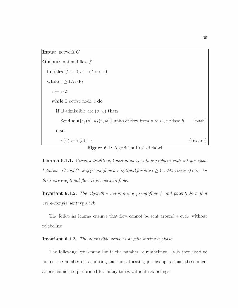
60

Input: network G

Output: optimal flow f

Initialize f ← 0, ε← C, π ← 0

while ε ≥ 1/n do

ε← ε/2

while ∃ active node v do

if ∃ admissible arc (v, w) then

Send min{ef (v), uf(v, w)} units of flow from v to w, update h {push}

else

π(v)← π(v) + ε {relabel}Figure 6.1: Algorithm Push-Relabel

Lemma 6.1.1. Given a traditional minimum cost flow problem with integer costs

between −C and C, any pseudoflow is ε-optimal for any ε ≥ C. Moreover, if ε < 1/n

then any ε-optimal flow is an optimal flow.

Invariant 6.1.2. The algorithm maintains a pseudoflow f and potentials π that

are ε-complementary slack.

The following lemma ensures that flow cannot be sent around a cycle without

relabeling.

Invariant 6.1.3. The admissible graph is acyclic during a phase.

The following key lemma limits the number of relabelings. It is then used to

bound the number of saturating and nonsaturating pushes operations; these oper-

ations cannot be performed too many times without relabelings.

61

Lemma 6.1.4. A node potential can increase O(n) times during a phase.

Between saturating pushes on an arc, both of its endpoints must be relabeled at

most once. This leads to the next lemma.

Lemma 6.1.5. There are O(mn) saturating pushes per phase.

Using a potential function argument, the next lemma bounds the number of

nonsaturating pushes of the generic push-relabel algorithm. By choosing the ad-

missible arcs more carefully, it is possible to reduce the bound on the number of

nonsaturating pushes to O(n3).

Lemma 6.1.6. There are O(mn2) nonsaturating pushes per phase.

The bottleneck operation is performing nonsaturating pushes. The (amortized)

cost per nonsaturating push can be reduced to O(log n) using the dynamic tree

data structure developed by Sleator and Tarjan [51]. The main idea is to perform

a succession of pushes along a single path in one operation. The dynamic tree data

structure maintains a forest of admissible arcs and their residual capacities. Instead

of just pushing flow along a single admissible arc, say (v, w), we push flow along

arc (v, w) and then along the tree path from w to its root. Using the dynamic tree

data structure, this push operation takes only O(logn) (amortized) time instead of

possibly O(n). After a nonsaturating push on arc (v, w), we add it to the forest. It

is still admissible, and we know its residual capacity. The results are summarized

in the following theorem.

Theorem 6.1.7. The generic push-relabel algorithm requires O(mn2 logC) time

and O(mn logC) time using the dynamic tree data structure.

62

6.2 Push-Relabel for Generalized Flows

Algorithm Rounded Push-Relabel (RPR) is a generalized flow analog of Goldberg

and Tarjan’s [24] push-relabel algorithm for the minimum cost flow problem, which

is described in Section 6.1. Conceptually, RPR runs the minimum cost flow al-

gorithm with costs c = − logb γ and fixes an error parameter ε = 1n

log2 b, where

b = (1 + ξ)1/n. We define an admissible arc and the admissible graph as before.

An active node is a node with positive residual excess and a residual path to the

sink. We note that if no such residual path exists and an optimal solution sends

flow through this node, then it does not reach the sink. So, it is safe to disregard

this useless excess.

Algorithm RPR maintains a flow h and node labels µ. The algorithm repeatedly

selects an active node v. If there is an admissible arc (v, w) emanating from node v,

RPR pushes δ = min{eh(v), uh(v, w)} units of flow from node v to w. If δ = uh(v, w)

the push is called saturating; otherwise it is nonsaturating. If there is no such

admissible arc, RPR increases the label of node v by a factor of 2ε = b1/n; this

corresponding to an additive potential increase for minimum cost flows. This process

is referred to as a relabel operation. Increasing the label of node v can create

new admissible arcs emanating from v. However, to ensure that we maintain the

approximate complementary slackness conditions, we only increase the label by

a relatively small amount; this guarantees that we do not create residual flow-

generating cycles.

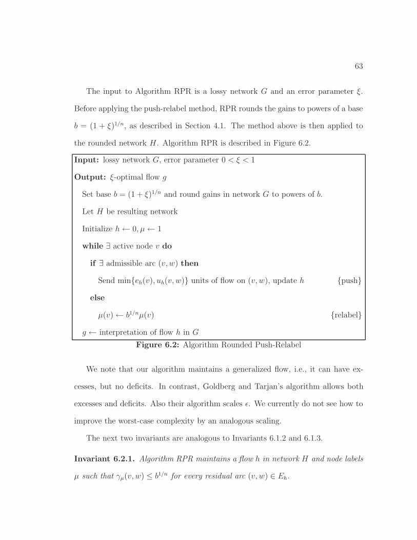
63

The input to Algorithm RPR is a lossy network G and an error parameter ξ.

Before applying the push-relabel method, RPR rounds the gains to powers of a base

b = (1 + ξ)1/n, as described in Section 4.1. The method above is then applied to

the rounded network H. Algorithm RPR is described in Figure 6.2.

Input: lossy network G, error parameter 0 < ξ < 1

Output: ξ-optimal flow g

Set base b = (1 + ξ)1/n and round gains in network G to powers of b.

Let H be resulting network

Initialize h← 0, µ← 1

while ∃ active node v do

if ∃ admissible arc (v, w) then

Send min{eh(v), uh(v, w)} units of flow on (v, w), update h {push}

else

µ(v)← b1/nµ(v) {relabel}

g ← interpretation of flow h in G

Figure 6.2: Algorithm Rounded Push-Relabel

We note that our algorithm maintains a generalized flow, i.e., it can have ex-

cesses, but no deficits. In contrast, Goldberg and Tarjan’s algorithm allows both

excesses and deficits. Also their algorithm scales ε. We currently do not see how to

improve the worst-case complexity by an analogous scaling.

The next two invariants are analogous to Invariants 6.1.2 and 6.1.3.

Invariant 6.2.1. Algorithm RPR maintains a flow h in network H and node labels

µ such that γµ(v, w) ≤ b1/n for every residual arc (v, w) ∈ Eh.

64

Proof. We prove by induction on the number of push and relabel operations. Ini-

tially all relabeled residual arcs have gain factors at most one. The push operation

only sends flow along arcs with relabeled gain above one; therefore only arcs with

relabeled gain below one can be added to the residual network. The relabel oper-

ation only applies to node v when there are no residual arcs (v, w) with relabeled

gain above one. The label of node v is increased by b1/n. The relabeled gain of

outgoing residual arcs can increase to at most b1/n. The relabeled gain of incoming

arcs decreases. The relabeled gain of other arcs do not change.

The next invariant relies on the fact that the network is rounded. It is needed

to ensure that the algorithm finds an optimal flow in the rounded network H.

Invariant 6.2.2. During Algorithm RPR, the admissible graph is acyclic.

Proof. We prove by induction on the number of push and relabel operations. Ini-

tially there are no admissible arcs, so the admissible graph is acyclic. A push

operation sends flow along an arc with relabeled gain exceeding one. The reversal

of this arc may be added to the residual network, but it is not admissible, as its

relabeled gain factor is less than one. Thus, pushes do not create admissible arcs,

so the admissible graph remains acyclic. The relabel operation increases the label

of some node, say v, by b1/n. This might create admissible arcs leaving v. All arcs

entering v have their relabeled gain decreased by b1/n. By Invariant 6.2.1, these arcs

now have relabeled gains at most one, and hence are inadmissible. Consequently,

the relabel operation does not create any directed admissible cycle passing through

node v.

65

Invariant 6.2.3. Algorithm RPR maintains a flow h in network H such that Hh

has no residual flow-generating cycles.

Proof. Let Γ be a residual cycle with γ(Γ) ≥ 1. By Invariant 6.2.1 all relabeled gains

in Γ are at most b1/n. By Invariant 6.2.2, not all of the arcs in Γ have relabeled

gain above one. Thus γµ(Γ) ≤ b1−1/n < b. Then γ(Γ) ≤ 1 since γ(Γ) = γµ(Γ) and

all gains are powers of b.

Lemma 6.2.4. Upon terminates, Algorithm RPR outputs a ξ-optimal flow g in

network G.

Proof. Invariant 6.2.3 and Theorem 2.3.7 imply that if the algorithm terminates

then the flow h is optimal in network H, since then there are no active nodes or

residual flow-generating cycles in Hh. By Corollary 4.1.2 the flow g is ξ-optimal in

G.

The following key lemma bounds the number of label increases. This yields a

good bound because by rounding the network, we were able to choose a large enough

base b.

Lemma 6.2.5. There are O(n3ξ−1 logB) relabels per node.

Proof. We show that the label of an active node cannot get too big. This limits

the number of relabelings. Let v be an active node. Let P be a v-t path in Hh,µ.

By Invariant 6.2.1 γµ(P ) ≤ b. By definition, γµ(P ) = µ(v)γ(P ) and γ(P ) ≥ B−n.

Thus, µ(v) ≤ bBn. Since each relabeling of node v increases its label by a factor of

66

b1/n, the number of times a node is relabeled is at most

logb1/n(bBn) = n+n2 logB

log b= O(n3ξ−1 logB).

As for the minimum cost flow problem, once we have a bound on the number

of relabeling operations, we can bound the number of saturating and nonsaturating

pushes.

Lemma 6.2.6. There are a total of O(mn3ξ−1 logB) saturating pushes.

Proof. We show below that between two consecutive saturating pushes on arc (v, w),

node v and node w must each be relabeled at least once. Combining this fact with

Lemma 6.2.5 implies that each arc is saturated at most O(n3ξ−1 logB) times.

Consider a saturating push on arc (v, w). At the time of the push, γµ(v, w) > 1,

since (v, w) is admissible. Before arc (v, w) can be saturated again, flow must be

pushed back along the reverse arc (w, v). At this time, γµ(w, v) > 1, or equivalently

γµ(v, w) < 1. So, between the original saturating push and the reverse push, node

w must have been relabeled at least once. At the time of the subsequent saturating

push on arc (v, w), γµ(v, w) > 1. Before this can happen, node v must have been

relabeled at least once.

Lemma 6.2.7. There are a total of O(mn4ξ−1 logB) nonsaturating pushes.

Proof. We prove the lemma using the potential function Φ =∑

v is active n(v), where

n(v) is the number of nodes reachable from v (including itself) in the admissible

67

graph. At the beginning of the algorithm Φ ≤ n, since initially there are no admis-

sible arcs. We now consider the effects of relabeling, saturating, and nonsaturating

push operations on the potential function.

After a saturating push on arc (v, w), node w might become active. This can

increase Φ by at most n(w) ≤ n. Lemma 6.2.6 implies that the total increase due

to saturating pushes is O(mn4ξ−1 logB).

Relabeling node v can create new admissible arcs leaving v, so n(v) can increase

by as much as n units. However, as in the proof of Invariant 6.2.2, after the re-

labeling, all arcs entering v are not admissible; thus n(w) does not increase for

any other node w. By Lemma 6.2.5, the total increase in Φ due to relabelings is

O(n4ξ−1 logB).

After a nonsaturating push on arc (v, w), we show that Φ decreases by at least

one unit. Since the push is nonsaturating, node v becomes inactive, and node w

might become active. The push decreases Φ by n(v) and might increase it by n(w).

Note that n(v) ≥ n(w)+1, since every node reachable in the admissible graph from

w is also reachable from v; moreover v is not reachable from w since Invariant 6.2.2

guarantees that the admissible graph is acyclic. Thus, Φ decreases by at least one

unit.

The potential function is initially at most n. It increases by O(mn4ξ−1 logB)

from saturating pushes and relabelings. Each nonsaturating push decreases the

potential function by at least one. The lemma follows, since Φ cannot become

negative.

68

If we implement the algorithm exactly as stated, it turns out that the bottleneck

computation is finding active nodes, since it requires O(m) time to determine which

nodes can reach the sink. Instead, we could only need recompute active nodes before

each relabeling operations. Between recomputations, we act as though all excess

nodes created are active. The proof of correctness remains valid even if RPR relabels

or pushes flow from inactive excess nodes. As noted earlier, nodes that cannot reach

the sink can be disregarded for the remainder of the algorithm. Thus, the number

of relabeling operations can be bounded as before; the bounds on the number of

pushes do not change either.

The real bottleneck computation is performing nonsaturating pushes. As for

the traditional minimum cost flow problem, the (amortized) time per nonsaturat-

ing push can be reduced to O(logn) using the dynamic tree data structure. One

might be worried that the dynamic tree data structure can not be used directly in

generalized networks, since it does not account for the gain factors. Fortunately,

all admissible arcs have relabeled gain factor above one. We choose to push the

same quantity of flow through every arc in the path. This creates additional node

excesses, but no deficits. Our analysis is not affected by the creation of additional

excess. This leads to the following theorem.

Theorem 6.2.8. In O(mn3ξ−1 logB) time Algorithm RPR computes a ξ-optimal

flow in network G.

69

6.3 Recursive Rounded Push-Relabel

Algorithm RPR computes ξ-optimal flows in O(mn3ξ−1 logB) time. However, it

does not compute optimal flows in polynomial time since the precision required to

apply Lemma 2.5.2 is ξ−1 = BO(m). Algorithm Recursive Rounded Preflow-Push

(RRPR) is a version of RPR that also incorporates error-scaling, as described in

Section 4.2. To ensure that the rounding is performed in lossy networks, RRPR

uses CancelCycles to eliminate flow-generating cycles. It computes ξ-optimal

flows in O(mn3 logB) log(1/ξ) time and optimal flows in O(m2n3 log2B) time.

The input to RRPR is a network G and an error parameter ξ. In each phase,

RRPR computes a 1/2-optimal flow in the relabeled residual network using Algo-

rithm RPR. The input to RPR is required to be a lossy network, so before each call

to RPR, Algorithm RRPR cancels all residual flow-generating cycles using proce-

dure CancelCycles, as described in Section 8.1. Algorithm RRPR is described

in Figure 6.3.

Theorem 6.3.1. Algorithm RRPR computes a ξ-optimal flow in network G in

O(mn3 logB) log(1/ξ) time. It computes an optimal flow in O(m2n3 log2B) time.

Proof. Each phase captures at least half of the remaining flow. Thus, after log(1/ξ)

phases, the flow is ξ-optimal. The bottleneck computation is calling Algorithm

RPR; by Theorem 6.2.8, each call requires O(mn3 logB) time. This says that we

compute ξ-optimal flows in the stated time bound. We can find an optimal flow

in the stated time bound by first computing a B−3m-optimal flow and then using

Lemma 2.5.2 to convert it into an optimal flow.

70

Input: network G, error parameter 0 < ξ < 1

Output: ξ-optimal flow g

Initialize g ← 0

repeat

(g′, µ)← CancelCycles(Gg)

g ← g + g′

g′ ← RPR(Gg,µ, 1/2)

g ← g + g′

until g is ξ-optimal

Figure 6.3: Algorithm Recursive Rounded Push-Relabel

6.4 Issues for a Practical Implementation

The push-relabel algorithm for the traditional maximum flow problem is currently

believed to be the most practical. We believe our generalized push-relabel algo-

rithm will also be practical. In some preliminary computational experiments, we

implemented a version of RRPR. The overwhelming bottleneck computation was

canceling flow-generating cycles. To avoid this bottleneck, we also implemented a

version of the RPR approximation scheme. We plan to investigate how the algo-

rithm’s performance will deteriorate as we require improved precision. Also, if we

require an optimal solution, we can determine an error parameter for which the RPR

algorithm is fast, and then use the resulting solution as a “warm start” for a gener-

alized network simplex algorithm. We plan to perform computational experiments

using data for the machine scheduling problem discussed in Section 1.3.

Chapter 7

Fat-Path

In this chapter we present a new Fat-Path variant for the generalized maximum flow

problem. It matches the best known complexity bound for computing approximate

flows, and it is much simpler than Radzik’s variant. First, we review the details of

the original Fat-Path capacity-scaling algorithm of Goldberg, Plotkin and Tardos

[20]. Next, we describe Radzik’s [49] Fat-Path variant. Finally, we present our new

Fat-Path variant.

7.1 Most-Improving Augmenting Path

In this section we describe a simple (but not the most efficient) version of the

Fat-Path capacity-scaling algorithm of Goldberg, Plotkin, and Tardos [20]. The

most-improving augmenting path algorithm [52] generalizes the maximum capacity

augmenting path algorithm for the traditional maximum flow problem, e.g. see [1].

71

72

This version can also be used to generate an initial flow whose value is within a

factor of m of the optimum in O(m) time.

The value of an augmenting path is the maximum amount of flow that can

reach the sink, while respecting the capacity limits, by sending excess from the first

node of the path to the sink. A most-improving augmenting path is an augmenting

path with the highest value. The algorithm repeatedly sends flow along most-

improving augmenting paths. Since these may not be highest gain augmenting

paths, this may creates residual flow-generating cycles. After each augmentation,

the algorithm cancels all residual flow-generating cycles, so that computing the next

most-improving path can be done efficiently. Intuitively, canceling flow-generating

cycles can be interpreted as rerouting flow from its current paths to highest-gain

paths, but not all of the rerouted flow reaches the sink.

Input: generalized network G

Output: optimal flow g

repeat

g′ ← CancelCycles(Gg)

g ← g + g′

Find a most-improving augmenting path P in Gg

Augment flow along P and update g

until g optimal

Figure 7.1: Algorithm Most-Improving Augmenting Path

Lemma 7.1.1. In O(m log(1/ξ)) iterations, the most-improving augmenting path

algorithm computes a ξ-optimal flow.

73

Proof. By Corollary 2.3.4, the optimal flow in a lossy network can be decomposed

into at most m augmenting paths. The algorithm selects the path that generates

the maximum amount of excess at the sink. Thus, each iteration captures at least a

1/m-fraction of the remaining flow. Since (1−1/m)m ≈ 1/e, the algorithm captures

at least half of the remaining flow after O(m) iterations, and the lemma follows.

We give a new and faster subroutine for computing a most-improving augment-

ing path in a lossy network. Our subroutine is based on Dijkstra’s shortest path

algorithm. For each node v, the algorithm maintains a label d(v). Upon termina-

tion of the algorithm, d(v) is the maximum amount of flow arriving at v that can

be sent from the source along a path; during the algorithm d(v) is always a lower

bound on this quantity. Our algorithm is identical to Dijkstra’s shortest path algo-

rithm, except in the way the labels are updated. The algorithm selects a new node

v with the largest value of d(v). Assuming d(v) represents the maximum amount

of flow we can send to v, then we could send it to node w along arc (v, w). The

amount that reaches w is γ(v, w)×min{d(v), u(v, w)}. This leads to updating d(w)

with max{γ(v, w)×min{d(v), u(v, w)}, d(w)} for all (v, w) ∈ E. The algorithm is

described in Figure 7.2.

The following invariant establishes the correctness of the procedure and can be

proved by induction. The proof is straightforward and analogous to Dijkstra’s.

Invariant 7.1.2. At any point during the algorithm, the label of each node in S is

optimal. Moreover, the label of each node in S is the maximum amount of flow that

can reach that node, provided that each internal node of the path lies in S.

74

Input: lossy network G

Output: d(v) = maximum amount of flow that can reach v along a path

Initialize ∀v ∈ V : d(v)← e(v), S = {v : d(v) > 0}

while S 6= ∅ do

v ← argmax{d(i) : i ∈ S}

S ← S ∪ {v}

for all (v, w) ∈ E do

cap = γ(v, w)×min{d(v), u(v, w)}

if d(w) < cap then

d(w)← cap, pred(w)← v

Figure 7.2: Subroutine Finding a Most-Improving Augmenting Path

A straightforward implementation using Fibonacci heaps, as in the Fredman-

Tarjan [17] implementation of Dijkstra’s algorithm, implies the following theorem.

Theorem 7.1.3. There exists a O(m + n logn) time algorithm to find a most-

improving path in a lossy network.

Actually, subsequent to this thesis, Wayne discovered that the same ideas can

be used to find a most-improving generalized augmenting path. However, the com-

putation is more complicated. Essentially, he replaces our Dijkstra variant with

an analogous variant of a two variable per inequality feasibility detector. This is

the first known purely “augmenting path” style algorithm for the problem that is

polynomial. It repeatedly sends flow only along augmenting paths and GAPs.

75

Finding a Good Initial Flow. Our approximation algorithms for the general-

ized maximum flow problem need reasonably good estimates of the optimum value;

otherwise they may take as long as the exact algorithms. Radzik [49] proposed an

O(m)SP (m,n) time greedy augmentation algorithm that finds a flow whose value

is within a factor of n of the optimum. Alternatively, we can find a flow whose value

is within a factor m of the optimum in O(m+ n log n) time. By Corollary 2.3.4, a

most-improving augmenting path gives such a flow.

Corollary 7.1.4. In O(m + n log n) time we can determine an initial parameter

∆0 which satisfies OPT(G) ≤ ∆0 ≤ mOPT(G).

Remark 7.1.5. In contrast, for the minimum cost flow problem, it is NP-hard

to find a most-improving cycle. Although many minimum cost flow algorithms

have generalized flow analogs, it is very unlikely that finding a most-improving

augmenting path will have a proper analog for the minimum cost flow problem.

However, by solving a sequence of assignment problems, Baharona and Tardos [4]

showed how to efficiently find a collection of cycles whose value is at least as good

as the most-improving cycle.

7.2 Fat-Path

Now, we review the original Fat-Path algorithm and analysis of Goldberg, Plotkin,

and Tardos [20]. The bottleneck computation in the most-improving augmenting

path algorithm is canceling flow-generating cycles, which is done after each augmen-

tation. The main idea of the Fat-Path algorithm is to perform many augmentations,

76

before cycle-canceling. The Fat-Path algorithm can be viewed as a generalized flow

analog of Orlin’s [45] capacity-scaling minimum cost flow algorithm, which, in turn,

is a variant of Edmonds and Karp’s [13] algorithm. The underlying idea is to send

excess to the sink along augmenting paths with sufficiently large capacity. A δ-fat

path is a residual path that has enough capacity to increase the excess at the sink

by at least δ units of flow, given sufficient excess at the first node of the path.

The Fat-Path algorithm does not necessarily send flow along overall highest gain

augmenting paths. So, periodically it cancels all residual flow-generating cycles, so

that computing subsequent fat-paths can be done efficiently.

The input to the Fat-Path algorithm is a network G and error parameter ξ.

The Fat-Path algorithm solves the generalized maximum flow in phases. A phase

is characterized by a scaling parameter ∆, which provides an upper bound on

the excess discrepancy, i.e., the difference between the value of the current flow

and the value of the optimal flow. We initialize ∆, as in Corollary 7.1.4, so that

OPT(G) ≤ ∆ ≤ mOPT(G). Each phase decreases ∆ by a factor of two. When

∆ is sufficiently small, we will show that we have an approximately optimal flow.

Each phase consists of two components: canceling all residual flow-generating cy-

cles and finding fat-paths. At the beginning of a phase, all residual flow-generating

cycles are canceled, using procedure CancelCycles, as described in Section 8.1.

Next, procedure FatAugmentations, which we describe in Section 7.3, is used to

repeatedly augment flow along δ-fat paths, where δ = ∆/(2m), until no such paths

remain. At this point, ∆ is decreased by a factor of two, and a new phase begins.

We describe the Fat-Path algorithm in Figure 7.3.

77

Input: network G, error parameter 0 < ξ < 1

Output: ξ-optimal flow g

Initialize g ← 0 and ∆ so that OPT(G) ≤ ∆ ≤ mOPT(G)

while ∆ > ξ|g| do

(g′, µ)← CancelCycles(Gg)

g ← g + g′

g′ ← FatAugmentations(Gg,µ,∆/(2m)) {OPT(Gg)− |g′| ≤ ∆/2}

g ← g + g′

∆← ∆/2

Return g

Figure 7.3: Algorithm Fat-Path

Procedure FatAugmentations is the core of the Fat-Path algorithm. It ef-

ficiently determines a flow with relatively small excess discrepancy. The following

lemma summarizes the result of procedure FatAugmentations. We defer its

proof until Section 7.3. Once we establish this key lemma, the rest of the analysis

is straightforward.

Lemma 7.2.1. If Gg,µ is a lossy network, then in O((m+n log n)(n+OPT(Gg)/δ))

time, procedure FatAugmentations(Gg,µ, δ) outputs a flow g′ of value at least

OPT(Gg)−mδ.

The following invariant says that ∆ acts as a good proxy for the excess discrep-

ancy, i.e., when ∆ is small then so is the excess discrepancy.

78

Invariant 7.2.2. The parameter ∆ remains an upper bound on the excess discrep-

ancy, i.e., OPT(G)− |g| ≤ ∆.

Proof. We initialize g = 0 and OPT(G) ≤ ∆. The excess discrepancy can only

decrease throughout the algorithm, so we only need to worry about what happens

when ∆ is decreased. By Lemma 7.2.1, FatAugmentations returns a flow g′ in

Gg whose value is at least OPT(Gg) − mδ = OPT(Gg) − ∆/2. Thus g + g′ has

excess discrepancy at most ∆/2, so when ∆ is halved, it remains an upper bound

on the excess discrepancy.

The next guarantees that upon termination the flow is of the desired quality.

Lemma 7.2.3. Upon termination, the flow g is ξ-optimal.

Proof. Upon termination, ∆ ≤ ξ|g| ≤ ξOPT(G). By Invariant 7.2.2 we also have

OPT(G)− |g| ≤ ∆. The lemma combines these two inequalities.

The next lemma bounds the number of phases.

Lemma 7.2.4. There are O(log(m/ξ)) phases.

Proof. Initially ∆ ≤ mOPT(G). We show that the algorithm will terminate before

∆ ≤ ξOPT(G)/2. The lemma then follows, since ∆ halves in each phase. If

∆ ≤ ξOPT(G)/2, then we have

2∆ ≤ ξOPT(G) ≤ ξ∆ + ξ|g| ≤ ∆ + ξ|g|,

where the second inequality follows from Invariant 7.2.2. This implies that ∆ ≤ ξ|g|,

which is precisely the stopping condition.

79

Theorem 7.2.5. In O(mn2 logB) log(1/ξ) time The Fat-Path algorithm computes

a ξ-optimal flow.

Proof. Lemma 7.2.3 and Theorem 4.1.1 ensure the flow returned is of the de-

sired quality. By Lemma 7.2.4 there are O(log(m/ξ)) phases. The complexity

of each phase is dominated by procedures CancelCycles and FatAugmenta-

tions. By Theorem 8.1.10, CancelCycles requires O(mn2 log n logB) time per

phase. FatAugmentations requiresO(m(m+n logn)) time per phase; this follows

from Lemma 7.2.1, since Invariant 7.2.2 guarantees that the algorithm maintains

∆ ≥ OPT(Gg) and we choose δ = ∆/(2m).

7.3 Fat Augmentations

In this section, we review the FatAugmentations procedure of Goldberg, Plotkin,

and Tardos [20]; it is the core of their Fat-Path algorithm. The purpose of this

procedure is to repeatedly augment flow along δ-fat paths, until no such paths

remain. At this point, we can show that the excess discrepancy is relatively small.

The procedure is based on Dijkstra’s shortest path algorithm.

Definitions and Intuition. A highest-gain δ-fat path is a highest gain path,

among all δ-fat paths. The FatAugmentations procedure repeatedly augments

flow along highest-gain δ-fat paths. By only selecting such paths, FatAugmenta-

tions is able to find subsequent δ-fat paths efficiently.

80

A δ-fat arc is an arc that participates in some δ-fat path. Consider a highest-

gain augmenting path from some node to the sink. Either this path is δ-fat or there

is (at least) one bottleneck arc, say (v, w), that would be saturated when flow is

augmented along this path. The capacity of this bottleneck arc (v, w) times the gain

of the part of the path from v to the sink, say P1, is less than δ, i.e., u(v, w)γ(P1) < δ.

In this case we say that (v, w) is a critical arc. Critical arcs cannot be δ-fat. The

main idea of the FatAugmentations subroutine is to disregard critical arcs, while

constructing a highest-gain δ-fat path.

Let Gδg denote the subgraph induced by residual δ-fat arcs. To improve the effi-

ciency for repeatedly finding highest-gain δ-fat paths, FatAugmentations main-

tains node labels µ so that Gδg,µ is a lossy network. This guarantees that there are

no flow-generating cycles in Gδg, and allows us to use a Dijkstra style computation

instead of a Bellman-Ford style one. Note that non δ-fat arcs may have relabeled

gain above one. After sending flow along a highest-gain δ-fat path, we will show

that disregarded arcs do not become δ-fat. This fact will ensure that Gδg,µ remains

a lossy network after augmenting flow along a highest-gain δ-fat path.

The Procedure. The input to FatAugmentations is a lossy network G and

fatness parameter δ. The output is a flow g such that Gδg,µ is a lossy network with

no augmenting paths. Analogous to Dijkstra’s algorithm, the procedure constructs

not just a single highest-gain δ-fat path, but a highest gain δ-fat tree, i.e., a tree

rooted at the sink such that the tree path from any node to the sink is δ-fat, and

has the highest gain among all such paths. A highest-gain δ-fat tree corresponds

81

to a shortest path tree in Gδg,µ, using costs c = − log γ. Since Gδ

g,µ is a lossy

network all arc costs are nonnegative and we construct the tree with a Dijkstra

style computation. The difficulty is that we do not know which arcs are δ-fat ahead

of time, i.e. we do not know the network Gδg,µ on which we wish to apply Dijkstra’s

algorithm! Surprisingly, FatAugmentations is able to simultaneously disregard

non δ-fat while running Dijkstra’s algorithm on the proper network.

For each node v ∈ V , we denote the maximum gain of the δ-fat v-t path found

so far by node label Gain(v). As in Dijkstra’s algorithm, at each iteration we find

a node v that has the largest Gain(v) among non-tree nodes and update the Gain

of its neighbors:

∀ u such that (u, v) ∈ Eg : Gain(u)← max{Gain(u), Gain(v)γµ(u, v)}

However, we should only perform the Dijkstra update for δ-fat arcs, as we build the

tree. Before performing the Dijkstra update, we disregard an arc if

ug,µ(u, v)γµ(u, v)Gain(v) < δ.

We will show that an arc is disregarded if and only if it is not δ-fat.

After the tree is constructed, we multiply the label of node v by Gain(v), so

that every tree arc has unit relabeled gain. Then we find a node in the tree with

positive excess, and augment flow along the δ-fat tree path. We will show that Gδg,µ

remains a lossy network. The method is then repeated until no such δ-fat paths

remain. Procedure FatAugmentations is described in Figure 7.4.

82

Input: lossy network G, fatness parameter δ

Output: flow g, labels µ such that Gδg,µ is a lossy network with no augmenting

paths

Initialize g ← 0, µ← 1

repeat

Initialize Gain(v)← 0 for all v 6= t, Gain(t)← 1, T ← ∅

while there are nodes not in T with nonzero Gain do

v ← node not in T with highest Gain

add arc (v, parent(v)) to T

for all nodes u such that (u, v) ∈ Eg do

if ug,µ(u, v)γµ(u, v)Gain(v) < δ then

disregard arc (u, v)

else

if Gain(u) < Gain(v)γµ(u, v) then

Gain(u)← Gain(v)γµ(u, v), parent(u)← v

Update µ(v)← µ(v)×Gain(v)

If there exists augmenting path in T , then send flow along path and update g

until Gg has no δ-fat paths

Figure 7.4: Subroutine Fat Augmentations

83

The following lemma says that in each while loop, FatAugmentations con-

structs a highest-gain δ-fat tree. It assumes that Gδg,µ is a lossy network. Invari-

ant 7.3.2 below guarantees that Gδg,mu remains a lossy network during the procedure.

Lemma 7.3.1. If Gδg,µ is a lossy network at the beginning of the while loop, then

it constructs a highest-gain δ-fat tree.

Proof. We show below that an arc is disregarded if and only if it is not δ-fat. Since

Gδg,µ is a lossy network, all δ-fat arcs have nonnegative length using lengths − log γµ.

Then, the while loop is an implementation of Dijkstra’s algorithm on the subgraph

induced by δ-fat arcs. Consequently, it constructs a highest-gain δ-fat tree.

Now, we show that an arc is disregarded if and only if it is not δ-fat. We prove

by induction on the number of arcs examined. Let (u, v) denote the arc currently

being examined. By induction, all previous arcs were disregarded if and only if they

were not δ-fat. Thus, the tree constructed so far is a highest-gain δ-fat subtree.

First, we consider the case when (u, v) is not disregarded. We show that (u, v)

is δ-fat. Since (u, v) is not disregarded, we have

ug,µ(u, v)γµ(u, v)Gain(v) ≥ δ.

Let P be the v-t path in the current highest-gain δ-fat subtree. Inductively, P is a

δ-fat path. Thus, (u, v) and P form a δ-fat path also, since Gain(v) = γ(P ).

Now, we consider the case when (u, v) is a δ-fat arc. By definition, there exists

a v-t path P1 such that (u, v) and P1 form a δ-fat path, i.e.,

ug,µ(u, v)γµ(u, v)∏e∈P1

γµ(e) ≥ δ. (7.1)

84

Let P2 be the v-t path in the current highest-gain δ-fat subtree. Since P1 is some

other δ-fat path from v to t, we have

Gain(v) =∏e∈P2

γµ(e) ≥∏e∈P1

γµ(e). (7.2)

Combining (7.1) and (7.2) we obtain ug,µ(u, v)γµ(u, v)Gain(v) ≥ δ, so we would not

disregard arc (u, v).

The following invariant ensures that at the beginning of the while loop, there are

no δ-fat arc with relabeled gain bigger than one. Thus, all arc costs are nonnegative

and we are in a position to run the Dijkstra’s variant.

Invariant 7.3.2. FatAugmentations maintains a lossy network Gδg,µ.

Proof. We prove by induction. The input network is assumed to be a lossy network.

Before augmenting flow, the δ-fat network is canonically relabeled so that Gg,µ is

a lossy network and highest-gain δ-fat paths have unit relabeled gain. Each δ-fat

augmentation is done along a highest-gain path, so only arcs with unit relabeled

gain can be added to the residual graph.

We still need to rule out the possibility that a non δ-fat arc with residual ca-

pacity becomes δ-fat. Let (u, v) be a non δ-fat arc with residual capacity before the

augmentation. Then, (u, v) was disregarded, i.e.,

ug,µ(u, v)γµ(u, v)Gain(v) ≥ δ.

Since augmentations are only along highest-gain δ-fat paths, Gain(v) does not in-

crease. Hence, (u, v) cannot become δ-fat.

85

Lemma 7.3.3. Procedure FatAugmentations(G, δ) outputs a flow g of value at

least OPT(G)−mδ.

Proof. Procedure FatAugmentations outputs a flow g such that Gδg has no aug-

menting paths or flow-generating cycles. Let g∗ be an optimal flow in G. We can

decompose the residual pseudoflow g∗ − g into at most m elementary pseudoflows,

as guaranteed by Theorem 2.3.3. All arcs in the decomposition are in Gg. The only

elementary flows that generate excess at the sink are augmenting paths and GAPs.

Therefore, it suffices to show that each of these elementary pseudoflows contributes

at most δ to the maximum excess that can be sent to the sink.

First we consider augmenting paths. By construction there are no δ-fat augment-

ing paths in Gg. Since each arc in the decomposition is in Gg, each augmenting path

can only bring less than δ units of excess to the sink.

Now we consider GAPs. Since Gδg is a lossy network, there are no flow-generating

cycles induced by δ-fat arcs in Gg. Since every arc in the decomposition is also in

Gg, every GAP in the decomposition has at least one arc in the flow-generating

cycle, say (v, w), that is not δ-fat. The amount of flow that the GAP can generate

at the sink is bounded above by the fatness of the (v, t) path in the GAP, which

is less than δ. Thus, each GAP can only bring less than δ units of excess to the

sink.

The next lemma bounds the number of fat-paths that need to be computed.

Lemma 7.3.4. During Procedure FatAugmentations(G, δ), there are at most

n+ OPT(G)/δ augmentations.

86

Proof. Each augmentation either uses up all of the excess at a node or increases the

excess at the sink by at least δ.

The procedure FatAugmentations can be implemented much like Dijkstra’s

shortest path algorithm. Using the Fredman-Tarjan [17] implementation with Fi-

bonacci heaps, we obtain the following lemma.

Lemma 7.3.5. Procedure FatAugmentations computes each highest-gain δ-fat

tree in O(m+ n log n) time.

7.4 Radzik’s Fat-Path Variant

The bottleneck computation in the original Fat-Path algorithm is canceling flow-

generating cycles. Radzik’s variant [49] reduces the bottleneck by canceling only

residual flow-generating cycles with sufficiently big gains. The CancelCycles

procedure quickly cancels flow-generating cycles with big gains, but requires signif-

icantly more time to cancel the remaining flow-generating cycles. For example, all

flow-generating cycles with gains exceeding 1 + 1/p(m), for any fixed polynomial

p(m), can be canceled in O(mn logB), but O(mn2 logB) time is required to cancel

all flow-generating cycles. The remaining flow-generating cycles are obscured by

appropriately decreasing the gain factors in the current computation. Since not

all of the flow-generating cycles are actually canceled, analyzing the precision of

the resulting solution is technically complicated. This idea leads to the following

theorem of Radzik [49]:

87

Theorem 7.4.1. In O(m2 +mn log logB) log(1/ξ) time Radzik’s Fat-Path variant

computes a ξ-optimal flow; in O(m3 logB + m2n logB log logB) time it computes

an optimal flow.

7.5 Rounded Fat-Path

In this section we present a new Fat-Path variant. Our variant runs the Fat-Path

algorithm in the rounded network. This allows us to obtain an improved complexity

bound on the CancelCycles procedure, which is the bottleneck computation. By

canceling all flow-generating cycles, we overcome the technical difficulties associated

with Radzik’s variant. Our rounding is done in a network with no residual flow-

generating cycles, which makes the quality of the resulting solution easy to analyze.

Subsequent calls to the CancelCycles procedure are performed in a pre-rounded

network, which enables us to achieve an improved complexity bound.

7.5.1 Rounded Fat-Path

Algorithm Rounded Fat-Path (RFP) runs the original Fat-Path algorithm in a

rounded network. The input is a lossy network G and an error parameter ξ. First,

RFP rounds down the gains to powers of b = (1 + ξ)1/n, as described in Section 4.1.

We note that if G is a lossy network, then so is the rounded network, which we

denote by H. Then Algorithm RFP runs the original Fat-Path algorithm on the

rounded network. Algorithm RFP is given in Figure 7.5.

88

Input: lossy network G, error parameter 0 < ξ < 1

Output: 2ξ-optimal flow g

Set base b = (1 + ξ)1/n and round gains in network G to powers of b

Let H be resulting network

h← Fat-Path(H, ξ)

Return g ← interpretation of h in G

Figure 7.5: Algorithm Rounded Fat-Path

Theorem 7.5.1. If G is a lossy network then Algorithm RFP outputs a 2ξ-optimal

flow in O(m2 +mn logB log(1/ξ)) log(1/ξ) time.

Proof. Theorem 7.2.5 implies that the flow h is ξ-optimal in network H. Theo-

rem 4.1.1 says that the interpretation of the flow h in the original network is a

2ξ-optimal flow.

As in the proof of Theorem 7.2.5, the bottleneck computations are procedures

FatAugmentations and CancelCycles. As before, FatAugmentations re-

quires O(m2) per invocation. Since all of the gain factors are powers of b, The-

orem 8.1.10 says that CancelCycles requires O(mn logC) time per invocation,

where C ≤ n2ξ−1 logB.

7.5.2 Recursive Rounded Fat-Path

Algorithm RFP computes a ξ-optimal flow in O(m2 +mn log logB) time when ξ−1

is O(p(m)) for any polynomial p(m), but does not compute optimal flows faster

than the original Fat-Path algorithm. Our new recursive version computes nearly

89

optimal and optimal flows faster than the original Fat-Path algorithm. The idea is

that we can compute a ξ-optimal flow from two√ξ-optimal flows, as described in

Section 4.1. In each recursive call, we re-round the network. The benefit is roughly

to decrease the average value of C from O(n2ξ−1 logB) to O(n2 logB) because G

is a “pre-rounded” network.

The input to Algorithm Recursive Rounded Fat-Path (RRFP) is a network G,

an upper bound ∆ ≥ OPT(G) on the optimal value and an error parameter ε.

We assume the gain factors in the input network have already been pre-rounded

to powers of (1 + ε2)1/n; this will be the case when the algorithm is called recur-

sively. The output is a flow of value at least OPT(G)− ε∆. With appropriate input

parameters we can use RRFP to find a ξ-optimal flow in G. Algorithm RRFP

first cancels all residual flow-generating cycles. If the error parameter is sufficiently

course, FatAugmentations efficiently returns a flow of the desired precision. Oth-

erwise, we round gain factors in the relabeled residual graph Gg,µ down to powers

of b = (1 + ε/2)1/n. Let H denote the resulting rounded network. Now RRFP

recursively calls itself with network H and error parameter√ε/2. Let h denote the

resulting flow. Then RRFP recursively calls itself again in the resulting residual

network Hh with the same error parameter. Let h′ denote the resulting flow. Let

g′ denote the interpretation of flow h+ h′ in Gg. RRFP outputs the flow g+ g′; we

show below that it has the desired level of precision. Algorithm RRFP is described

in Figure 7.6.

The following lemma shows that RRFP outputs a flow of the desired quality.

90

Input: network G where gains are powers of (1+ε2)1/n, upper bound ∆ ≥ OPT(G),

error parameter 0 < ε < 1

Output: flow g with value at least OPT(G)−∆ε

(g, µ)← CancelCycles(G)

if ε > 1/2 then

g′ ← FatAugmentations(Gg,µ,∆ε/m) {OPT(Gg)− |g′| ≤ ∆ε}

g ← g + g′

else

Round relabeled gains down to powers of b = (1 + ε/2)1/n

Let H be resulting network

h← RRFP(H,∆,√ε/2) {OPT(H)− |h| ≤ ∆

√ε/2}

h′ ← RRFP(Hh,∆√ε/2,

√ε/2) {OPT(Hh)− |h′| ≤ ∆ε/2}

g′ ← interpretation of flow h+ h′ in Gg {OPT(Gg)− |g′| ≤ ∆ε}

g ← g + g′

Figure 7.6: Algorithm Recursive Rounded Fat-Path

Lemma 7.5.2. If ∆ ≥ OPT(G) and 0 < ε < 1 then RRFP(G,∆, ε) returns a flow

in network G of value at least OPT(G)−∆ε.

Proof. The proof is by induction on the depth of the recursion tree. At depth zero,

when ε > 1/2, by Lemma 7.3.3 FatAugmentations(Gg , µ,∆ε/m) returns a flow

g′ of value |g′| ≥ OPT(Gg)−m(∆ε/m) = OPT(Gg)−∆ε. Hence

OPT(G)− |g + g′| = OPT(Gg)− |g′| ≤ ∆ε.

91

Otherwise when ε ≤ 1/2

OPT(G)− |g + g′| ≤ OPT(G)− |g| − |h| − |h′|

≤ (1− ε/2) OPT(G) + ∆ε/2− |g| − |h| − |h′|

≤ (1− ε/2) OPT(Gg)− |h| − |h′|+ ∆ε/2

≤ OPT(H)− |h| − |h′|+ ∆ε/2

= OPT(Hh)− |h′|+ ∆ε/2

≤ ∆ε/2 + ∆ε/2 = ∆ε.

The first inequality follows since flow interpretation can only create additional ex-

cesses. The second inequality holds since OPT(G) ≤ ∆ by Invariant 7.2.2. Since

H is the rounded network, the fourth inequality holds by Theorem 4.1.1. The final

inequality follows by induction on the second recursive call.

We need to check that the inductive hypothesis for the second recursive call is

valid, i.e., ∆√ε/2 ≥ OPT(Hh). This follows by induction on the first recursive call,

since it outputs a flow h that satisfies OPT(Hh) = OPT(H)− |h| ≤ ∆√ε/2. Also,

we need to check that the inductive hypothesis for the first recursive call is valid.

It is satisfied since ∆ ≥ OPT(G) ≥ OPT(H).

Now, we can bound the running time of algorithm RRFP.

Lemma 7.5.3. If ε−1 = BO(m) then in O(m2 + mn log logB) log(1/ε) time Algo-

rithm RRFP(G,∆, ε) terminates.

Proof. The bottleneck computations are procedures CancelCycles and FatAug-

mentations. There are log log ε−1 levels in the recursion tree. RRFP calls Fa-

92

tAugmentations only at depth zero in the recursion tree. Thus, there are log(1/ε)

calls to FatAugmentations; Lemma 7.2.1 implies that each call requires O(m2)

time.

Now, we bound the time due to calls to CancelCycles. During an invocation

of RRFP with error parameter ε, RRFP calls CancelCycles once and recursively

calls RRFP twice with error parameter√ε/2. Since all of the gains are powers of

(1 + ε2)1/n, the call to CancelCycles requires O(mn log n log(nC)) where C =

n2ε−2 logB. Let T (m,n, ε) be an upper bound on the time required to execute

RRFP(G, ε,∆). Then T solves the recurrence:

T (m,n, ε) = O(mn log n log

(n3 logB

ε2

))+ 2T (m,n,

√ε/2). (7.3)

Radzik [49] showed that

T (m,n, ε) = O(mn log n log(n logB) log ε−1) +O(mn log n log ε−1 log log ε−1)

solves the recurrence (7.3). When ε−1 is BO(m), which will be the case even to com-

pute optimal flows, this simplifies to: T (m,n, ε) = O(mn log n log(m logB) log ε−1).

Theorem 7.5.4. In O(m2 + mn log logB) log(1/ξ) time Algorithm RRFP com-

putes a ξ-optimal flow. An extra O(mn2 logB) preprocessing time is required if

G has residual flow-generating cycles. Algorithm RRFP computes an optimal flow

in O(m3 logB +m2n logB log logB) time.

Proof. To compute a ξ-optimal flow, we initialize ∆ with a value ∆0 that satisfies

OPT(G) ≤ ∆0 ≤ mOPT(G). This can be done efficiently as described in Corol-

93

lary 7.1.4. By Lemma 7.5.2, the flow g that Algorithm RRFP(G,∆0, ξ/n) returns

satisfies:

|g| ≥ OPT(G)− (ξ/n)∆0 ≥ (1− ξ) OPT(G).

The complexity bound for computing approximate flows follows from Lemma 7.5.3.

To compute an optimal flow, it suffices by Lemma 2.5.2 to compute a B−3m-optimal

flow.

Complexity Bounds. The original Fat-Path variant of Goldberg, Plotkin, and

Tardos [20] solves the generalized maximum flow problem in O(m2n2 log2B) time.

It computes ξ-optimal flows in O(mn2 logB) log(1/ξ) time. Radzik [48] provided a

strongly-polynomial complexity of O(m2n) log(1/ξ) time for computing ξ-optimal

flows. Radzik’s [49] Fat-Path variant computes optimal flows in O(m3 logB +

m2n logB log logB) time and ξ-optimal flows in O(m2+mn log logB) log(1/ξ) time.

Our Fat-Path variant matches these best known worst-case complexity bounds.

Chapter 8

Canceling Flow-Generating Cycles

In this chapter we describe a method for converting one generalized flow into another

generalized flow whose residual graph contains no flow-generating cycles. In the

process additional excesses, but no deficits, may be created. By eliminating flow-

generating cycles, we can subsequently perform many generalized flow computations

more efficiently. The method was first used by Goldberg, Plotkin, and Tardos [20]

in their Fat-Path algorithm.

Our procedure is a variant of the CancelCycles procedure of [20]. With our

variant, we ensure an additional property: the node potentials change by only rela-

tively small amounts. This new property is useful for improving the complexity of

some generalized flow algorithms, including the primal-dual algorithm described in

Chapter 5. Also, Radzik [48] showed that with slight modifications, CancelCy-

cles runs in strongly polynomial-time; our variant allows a simpler proof of this

fact.

94

95

8.1 Cancel Cycles

In this section, we review the CancelCycles procedure of Goldberg, Plotkin, and

Tardos [20]. The basic approach is to repeatedly cancel residual flow-generating cy-

cles, i.e., send flow along a cycle, until one (or more) residual arcs become saturated.

By canceling flow-generating cycles, we may create additional node excesses, but

no deficits. This is the generalized flow analog of Klein’s [40] minimum cost flow

cycle-canceling algorithm with costs c = − log γ. Using this cost function, negative

cost cycles correspond to flow-generating cycles.

Canceling arbitrary negative cost cycles may result in an exponential-time al-

gorithm. Goldberg and Tarjan [23] obtained a polynomial-time minimum cost flow

algorithm by repeatedly canceling the residual cycle with the minimum mean cost;

recall the mean cost of a cycle Γ is µ(Γ) = c(Γ)/|Γ|, where c(Γ) =∑

e∈Γ c(e). Gold-

berg and Tarjan [23] also designed a more efficient cycle-canceling algorithm called

Cancel-and-Tighten; the crucial idea is to maintain node potentials and only

approximate the strategy of canceling minimum mean cycles.

The CancelCycles procedure of Goldberg, Plotkin, and Tardos [20] adapts

the Cancel-and-Tighten algorithm to generalized flows, using the cost function

c = − logb γ, for some base b > 0. CancelCycles is divided into cost-scaling

phases. In each ε-phase, the procedure maintains a generalized flow g and node

potentials π that satisfy the ε-complementary slackness conditions:

∀(v, w) ∈ Gg : cπ(v, w) = c(v, w)− π(v) + π(w) ≥ −ε. (8.1)

96

The node potentials are analogous to the node labels described in Section 2.3.2; the

node label corresponding to π(v) is µ(v) = bπ(v)−π(t), so that µ(t) is normalized to

one.

Remark 8.1.1. If g and π are 0-complementary slack then Gg,µ is a lossy network

because

∀(v, w) ∈ Gg : γµ(v, w) = γ(v, w)µ(v)/µ(w) = γ(v, w) bπ(v)−π(w) ≤ 1

where the last inequality follows from the definition of 0-complementary slackness.

There is a very close connection between the ε-complementary slackness condi-

tions and minimum mean cost cycles. Given a generalized flow g, we define ε(g)

to be the minimum value of ε for which g is ε-complementary slack for some node

potentials π. That is

ε(g) = minπ{ε : g, π satisfies (8.1)} .

With respect to g, we denote the value of the minimum mean cost residual cycle by

µ(g) = min {µ(Γ) : Γ ∈ Gg}

The strong duality between ε-complementary slackness and minimum mean cost

cycles is captured by the following lemma.

Lemma 8.1.2. Let g be a non-optimal flow. Then ε(g) = −µ(g).

Proof. The lemma follows immediately from linear programming strong duality. We

give a more direct proof.

97

Suppose g and π are ε-complementary slack. By definition, the reduced cost of

every residual arc is at least −ε, and hence the mean reduced cost of any cycle is at

least −ε. Thus, µ(g) ≥ −ε(g), since the mean cost of a cycle is equal to the mean

reduced cost of a cycle.

Now, we show µ(g) ≤ −ε(g). Let Γ be a residual cycle in Gg that has minimum

mean cost value µ(g) Suppose that we replace each arc cost c(v, w) by c(v, w) =

c(v, w)−µ(g). This increases the mean costs of every residual cycle by−µ(g). Hence,

Γ now has zero (reduced) cost and there are no negative (reduced) cost residual

cycles in Gg, with respect to the updated costs. Let π(v) denote the cheapest costs

from node v to the sink. using costs c. The shortest path optimality conditions

imply

∀(v, w) ∈ Eg : cπ(v, w) = c(v, w)− π(v) + π(w) ≥ 0.

In other words, g and π are −µ(g)-complementary slack. Thus ε(g) ≥ −µ(g).

Remark 8.1.3. Lemma 8.1.2 implies that it is possible to compute ε(g) by com-

puting the minimum mean cost cycle value. This can be done in O(mn) time. See

Section 2.2.2 for more details.

During a phase, CancelCycles maintains a flow g and node potentials π.

Instead of repeatedly canceling minimum mean cost cycles, it repeatedly cancels

totally negative cycles, until no such cycles remain. A totally negative cycle is a

residual cycle for which every arc has negative reduced cost. After an ε-phase, new

node potentials are computed, and the error parameter ε is decreased by a factor

of (1 − 1/n). Initially we choose ε = C = maxe∈E c(e), and when ε is sufficiently

98

small, we show that there are no residual flow-generating cycles. Procedure Can-

celCycles is described in Figure 8.1.

Input: network G

Output: flow g and labels µ such that Gg,µ is a lossy network

Initialize g ← 0, π ← 0, c← − logb γ, ε← C

while ∃ negative cost residual cycle in Gg do

Compute potentials π that are ε-complementary slack with g

Cancel all totally negative cycles in Gg and update g

ε← (1− 1/n)ε

µ(v)← bπ(v)−π(t)

Figure 8.1: Subroutine Cancel Cycles

Invariant 8.1.4. In the first step of a phase in CancelCycles there exist poten-

tials π that are ε-complementary slack with the current flow. Also, ε-complementary

slackness is preserved while canceling totally negative cycles.

Proof. We prove both claims together by induction. The lemma is true at the

beginning of the first phase since g = 0 and π = 0 are ε-complementary slack for

ε = C.

First, we show that canceling a totally negative cycle maintains ε-complementary

slackness. Canceling a totally negative cycle may only add the reversals of these

cycle arcs into the residual network, and each of these reverse arcs has positive

reduced cost.

99

Now, we demonstrate the existence of potentials which are ε-complementary

slack with the current flow at the beginning of a phase. At the end of the previous

phase, ε was decreased by a factor of (1 − 1/n). At this point, by induction, all

residual arcs have reduced cost at least −ε. Also, since there are no totally negative

cycles, at least one arc in each residual cycle has nonnegative reduced cost. This

implies µ(g) ≥ −ε(1− 1/n). Lemma 8.1.2 asserts that there exists node potentials

that are ε(g)-complementary slack with the current flow g.

The next lemma says that at the beginning of a phase, we can compute the node

potentials efficiently.

Lemma 8.1.5. At the beginning of an ε-phase, we can find node potentials π that

are ε-complementary slack with the current flow g in O(m) time.

Proof. After canceling totally negative cycles in the previous phase, the subgraph

induced by negative reduced cost residual arcs is acyclic and induces a topological

ordering of the nodes o : V → {0, . . . , n−1} such that if (v, w) ∈ Gg and cπ(v, w) <

0 then (v, w) is a forward arc in the ordering, i.e., o(v) < o(w). We compute

the topological ordering o and increase the node potential π(v) by o(v)ε/n. This

increases the reduced cost of forward arcs by at least ε/n, and decreases the reduced

cost of backwards arcs by at most (n − 1)/n. All negative reduced cost residual

arcs are forward arcs in the ordering; now, these arcs have reduced cost at least

−(1 − 1/n)ε. All backwards arcs previously had nonnegative reduced cost; now

these arcs have reduced cost at least −(1− 1/n)ε.

100

The next two lemmas say that if ε is sufficiently small, then the current flow

has no residual flow-generating cycles. This can then be used to bound the number

of phases and serve as a stopping condition. As an alternate stopping condition.

CancelCycles directly checks for flow-generating (negative-cost) cycles. This

condition can be checked in O(mn) time with a shortest path computation, e.g.,

see Section 2.2.1. However, checking this condition may dominate the overall com-

plexity, so we only check for negative cost cycles every n iterations.

Lemma 8.1.6. Suppose that the costs c = − logb γ are integral for some b > 0. Let

g and π be ε-complementary slack for ε < 1/n. Then Gg has no flow-generating

cycles.

Proof. Let Γ be a cycle in Gg. Then c(Γ) = cπ(Γ) =∑

e∈Γ cπ(e) ≥ −nε > −1.

By assumption, the costs are integral. Hence c(Γ) ≥ 0, or equivalently, Γ is not a

flow-generating cycle.

Lemma 8.1.7. Suppose the gains are ratios of integers between 1 and B. Let g and

π be ε-complementary slack for ε < 1/(2nBn log b). Then Gg has no flow-generating

cycles.

Proof. Let T denote the maximum product of gain numerators on a simple cycle,

and note that T ≤ Bn. Let Γ be a cycle in Gg with γ(Γ) > 1. Then γ(Γ) ≥ 1+T−1.

This implies that its mean cost

µ(Γ) ≤ − logb(1 + T−1)n

=− log2(1 + T−1)

n log b≤ −1

2nT log b

101

where the last inequality follows by taking a Taylor expansion of log2(1 + x) for

x ≤ 1. Now, by Lemma 8.1.2,

ε ≥ ε(g) = −µ(g) ≥ −µ(Γ) ≥ 12nT log b

≥ 12nBn log b

Lemma 8.1.8. If the gains are given as ratios of integers between 1 and B then

CancelCycles requires O(n2 logB) phases. If the costs are integers no bigger

than C, it requires O(n log(nC)) phases.

Proof. Each phase decrease ε by a factor of (1 − 1/n). Thus, after O(n) phases,

ε decreases by at least a factor of two. Initially ε = C. If the costs c = − logb γ

are integers no bigger than C, then Lemma 8.1.6 implies that we can stop when

ε < 1/n. If the gains are ratios of integers between 1 and B, then Lemma 8.1.7

implies that we can stop when ε < 1/(2nBn log b). Note that C ≤ logbB.

Now, we give a complexity bound for canceling totally negative cycles. Each

time we cancel a totally negative cycle, we saturate at least one arc with negative

reduced cost, and we do not create any new such arcs. Thus, we cancel at most

m cycles per phase. Finding and canceling a single totally negative cycle, while

creating only excesses and no deficits, can easily be done in O(m) time. This leads

to a O(m2) time method. By marking nodes that do not participate in totally

negative cycles, we can improve the complexity to O(mn) time.

Using the dynamic tree data structure of Sleator and Tarjan [51], we can improve

the complexity bound further. One of the primitive dynamic tree operations is

102

pushing the same amount of flow along every arc in a tree path. In non-generalized

networks, we can also use the dynamic tree data structure to push flow around a

cycle that consist of a tree path plus one extra arc. CancelCycles pushes flow

around totally negative cycles; this means that each arc in the cycle has a relabeled

gain factor exceeding one, and we would want to push increasing amounts of flow

along each successive arc in the cycle. Thus, the dynamic tree data structure does

not apply directly. However, we can directly use the dynamic tree data structure

by abstracting the notion of canceling a cycle; we now allow excesses to be created

at several nodes when canceling a cycle. We note that this does not affect any of

our previous analysis. Since all arcs have relabeled gain above one, by pushing the

same amount of flow along every arc in the cycle, we create excesses at every cycle

node. This idea leads to the following lemma from [20].

Lemma 8.1.9. Canceling all totally negative cycles requires O(m logn) time.

Theorem 8.1.10. If the gains are given as ratios of integers between 1 and B then

CancelCycles requires O(mn2 logB) time. If the costs are integers no bigger

than C, it requires O(mn logC) time.

Proof. The bottleneck computation is canceling all totally negative cycles. By

Lemma 8.1.9, each phase requires O(m) time. The number of phases is given by

Lemma 8.1.8.

103

8.2 Our Cancel Cycles Variant

In this section, we describe a new variant of CancelCycles. Our variant ensures

that the node potentials change by only a relatively small amount while canceling

cycles. Our procedure uses two types of potential updating. With respect to a flow g,

loose updating is similar to the potential updating in the original CancelCycles

procedure. It requires O(m) time, but does not guarantee to decrease ε by the

maximum amount. If there are no totally negative cycles, it decreases ε by at least

a factor of (1 − 1/n). We also use tight updating, which updates ε = ε(g) and

computes potentials that are ε(g)-complementary slack with g. It reduces ε by the

maximum possible amount, but is relatively expensive. It involves computing a

minimum mean cost cycle and requires O(mn) time. We also introduce a third

type of potential updating which we call medium updating. It offers a middleground

between loose and tight updating. It is much cheaper than tight updating, yet more

effective than loose updating. The three types of potential updating are described

in more detail below.

The input to our CancelCycles variant, which we call CancelCycles2, is

a lossy network G. It is divided into cost-scaling phases. In each phase, the proce-

dure balances the amount of work between canceling totally negative cycles, loose

updating, and tight updating. As with CancelCycles procedure, in each ε-phase,

our procedure maintains a flow g and potential π that are ε-complementary slack.

The procedure begins a cost-scaling phase by performing tight updating. Next,

the algorithm cancels a minimum mean cost cycle. Then it alternates between the

104

following two operations: first it cancels all totally negative cycles, then it performs

loose updating. The procedure CancelCycles2 is described in Figure 8.2.

Input: network G

Output: flow g and potentials µ such that Gg,µ is a lossy network

Initialize g ← 0, π ← 0, c← − logb γ

while ∃ negative cost residual cycle in Gg do

tight update

Cancel the minimum mean cost residual cycle in Gg

repeat

Cancel all totally negative cycles in Gg and update g

loose update

until g and π are ε/2-complementary slack

µ(v)← bπ(v)−π(t)

Figure 8.2: Subroutine Cancel Cycles2

Tight Updating. Tight updating sets ε to ε(g) and finds new potentials π that

are ε(g)-complementary slack with the current flow g. This can be done with a single

minimum mean cost cycle computation [1]: there is a natural set of node potentials

associated with this computation, and they are ε(g)-complementary slack with the

flow g. However, these potentials are not good enough for our purposes; they may

be too large. For our analysis, we compute ε(g) and use this value to find new

potentials which are relatively small.

105

Lemma 8.2.1. Suppose g and π are ε-complementary slack. Then, there exists

node potentials p such that g and π + p are ε(g)-complementary slack and 0 ≤ p ≤

nε. Moreover, given ε(g), we can find such potentials p with a single shortest path

computation.

Proof. First, we compute ε(g) = −µ(g). Then, we define c : Eg → < by c(v, w) =

cπ(v, w) + ε(g), so that there are no negative cost cycles in Gg with respect to the

new cost function c. Let q(v) denote the value of the cheapest (possibly trivial)

residual path from v to any other node using costs c. Note that q(v) ≤ 0 for every

node v.

Now, we describe how to compute q efficiently. Consider the network Gg with

costs c. We add a new artificial sink t′ and zero cost arcs from every node to t′.

Since there are no negative cost cycles, we can compute q using a single shortest

path (from every node to t′) computation. The shortest path optimality conditions

imply:

∀(v, w) ∈ Eg : q(v) ≤ q(w) + c(v, w).

and

∀v ∈ V : 0 ≥ q(v) ≥ nmine∈Eg

c(e) ≥ n(ε(g)− ε) ≥ −nε

Consequently,

∀(v, w) ∈ Eg : cπ+q(v, w) = cπ(v, w)− q(v) + q(w)

= c(v, w)− ε(g)− q(v) + q(w)

≥ −ε(g).

106

The lemma then follows by choosing p = q + nε.

Additionally, it is easy to verify that after tight updating, each arc participating in

a minimum mean cost residual cycle has reduced cost equal to −ε(g), implying that

it is a totally negative cycle.

Loose Updating. Loose updating occurs when there are no more totally nega-

tive cycles. By increasing the potentials of a subset of nodes, we may create new

arcs with negative reduced cost, and hence new totally negative cycles. Cancel-

Cycles2 performs loose updating immediately after cancelling all totally negative

cycles. At this point, there are no totally negative cycles; this induces a topological

ordering of the nodes. We say i � j if there is an i-j residual path using only

negative reduced arcs. Let (v, w) be some residual arc with reduced cost below

−ε/2; the phase terminates if no such arc exists. Loose updating increases by ε/2

the potential of each node x � w.

The following invariant says that the procedure maintains a flow and node po-

tentials that are ε-complementary slack.

Invariant 8.2.2. During an ε-phase, the algorithm maintains a flow g and poten-

tials π that are ε-complementary slack.

Proof. At the beginning of a phase, π is chosen to be ε-complementary slack with g,

where ε = ε(g). We prove by induction that within an ε-phase, the procedure main-

tains this property. As in Invariant 8.1.4, ε-complementary slackness is preserved

when canceling totally negative cycles.

107

Now, we show that ε-complementary slackness is preserved during loose up-

dating. Loose updating occurs only when there are no totally negative cycles. It

increases the node potentials for some subset S of nodes which have no negative

reduced cost leaving arcs. This decreases the reduced cost of arcs leaving S and in-

creases the reduced cost of arcs entering S by ε/2. But all arcs leaving S previously

had nonnegative reduced cost, so after the loose update they have reduced cost at

least −ε/2.

Lemma 8.2.3. There are at most n loose updates per phase.

Proof. By Invariant 8.2.2, during an ε-phase the reduced cost of every residual arc

is at least −ε. Before a loose update, CancelCycles2 selects an arc (v, w) with

reduced cost less than −ε/2. After the potential update, all arcs entering w have

reduced cost at least −ε/2. Thus, there can be at most n loose updates per ε-phase,

as no new residual arcs with reduced cost less than −ε/2 are created.

Medium updating. We introduce a medium updating which is a middleground

between loose and tight updating. After cancelling all totally negative cycles, we

would ideally like to perform tight updating and compute ε(g) exactly. This is

computationally expensive, so instead our procedure uses loose updating. Loose

updating can be done in linear time, but it may not provide high quality node

potentials. We propose a practical alternative.

Medium updating finds a value ε′ that is close to ε(g), without spending the

time to find the actual minimum mean cost cycle. We only need to estimate ε(g)

in networks that have no totally negative cycles. We exploit this fact. To do

108

this efficiently, we imagine that, in addition to the original arcs, a zero cost link

exists between every pair of nodes. We can efficiently find a minimum mean cost

cycle in this modified network by computing a minimum mean cost path in the

acyclic network induced by only negative cost arcs, without explicitly considering

the imaginary zero cost arcs. Let ε′ denote the value of the minimum mean cost

cycle in the modified network. Clearly ε′ ≤ ε(g), and it is not hard to see that

ε′ ≥ (1 − 1/n)ε. We can binary search for ε′ using a shortest path computation in

acyclic graphs. This requires only O(m) time per iteration. If we were to determine

ε′ exactly, in O(n logB) iterations the search interval would be sufficiently small.

If the gains in the network are rounded to powers of b = (1 + ξ)1/n then O(logC)

iterations suffice, where C = O(nξ−1 logB). Since we are only estimating ε(g),

there is no need to compute ε′ exactly either.

The following lemma gives a weakly-polynomial bound on the number of phases.

Lemma 8.2.4. If the gains are given as ratios of integers between 1 and B then

CancelCycles2 requires O(n logB) phases. If the costs are integers no bigger

than C, it requires log(nC) phases.

Proof. Now, each phase decrease ε by a factor of at least two. The rest of the proof

is the same as in Lemma 8.1.8.

The next lemma gives a strongly-polynomial bound on the number of phases.

Radzik [48] showed that O(m logn) phases suffice. Radzik introduces a new aux-

iliary parameter δ; the value of δ at the beginning of a phase is defined as the

minimum cost of a cycle canceled from the beginning of the phase until the end

109

of the procedure. His analysis relies on showing that δ converges geometrically to

zero. Our new algorithm allows a simpler proof the strongly-polynomial complexity

bound. We show that after O(logn) phases a new arc becomes fixed, i.e., the value

of flow on this arc will not change during the rest of the procedure.

Lemma 8.2.5. CancelCycles2 requires O(m logn) phases.

Proof. Within an ε-phase, Lemma 8.2.3 says that the potential of a node increases

by at most nε/2 due to loose updating. Hence from the start of the ε-phase until

the termination of the procedure, a node’s potential increases by at most nε as a

result of loose relabeling, since ε halves in each phase.

Following an ε-phase, tight updating might increase node potentials in subse-

quent scaling-phases. Lemma 8.2.1 implies that in the next scaling-phase, a node

potential increases by at most nε/2. Since ε halves in each phase, this implies

a node’s potential increases by a total of at most nε during all subsequent tight

updatings.

Hence after the initial tight updating in an ε-phase, a node’s potential increases

by at most 2nε, until the algorithm terminates. Hence if an arc’s reduced cost is

smaller than −3nε (after the initial tight updating) in some ε-phase, then that arc

is fixed, as its reduced cost will remain below −ε throughout the procedure.

In each phase, the first cycle canceled is a minimum mean cost cycle, say Γ. Let

ε be the scaling parameter when Γ is cancelled and let ε′ be the scaling parameter

2 + log n phases later. Then

µ(Γ) = −ε ≤ −4nε′.

110

Hence, throughout the ε′-phase at least one arc (v, w) ∈ Γ has reduced cost as small

as −4nε′. But we pushed flow on (v, w) in the ε-phase, so it wasn’t fixed then. Thus

the arc (v, w) becomes fixed within O(log n) phases.

Theorem 8.2.6. If the gains are given as ratios of integers between 1 and B then

CancelCycles2 requires O(mn2 logB) time. If the costs are integers no big-

ger than C, it requires O(mn log n) time. In any case CancelCycles2 requires

O(m2n) time. Moreover, it outputs a flow g and node labels B−3n ≤ µ ≤ B3n such

that Gg,µ is a lossy network, where B is the biggest gain of a residual arc in the

original network.

Proof. The number of phases is bounded by Lemma 8.2.4 and Lemma 8.2.5. By

Lemma 8.2.3 we cancel all totally negative cycles at most n times per phase. This

is the bottleneck computation; by Lemma 8.1.9, it requires O(mn log n) time per

phase.

Now we provide a bound on how much the potentials can increase. As in the

proof of Lemma 8.2.5, within an ε-phase, a node potential can increase by at most

nε due to tight updating, and by at most nε/2 due to loose updating. Since ε

halves in each phase, this implies that a node potential increases by at most 3nε

throughout the entire procedure. Initially π = 0, g = 0, and ε = ε(g) ≤ logb B. Thus

0 ≤ π ≤ 3n logb B. The theorem then follows, since the node label corresponding

to π(v) is µ(v) = bπ(v)−π(t).

Bibliography

[1] R. K. Ahuja, T. L. Magnanti, and J. B. Orlin. Network Flows: Theory, Algo-rithms, and Applications. Prentice Hall, Englewood Cliffs, NJ, 1993.

[2] R. K. Ahuja, K. Mehlhorn, J. B. Orlin, and R. E. Tarjan. Faster algorithmsfor the shortest path problem. Journal of the ACM, 37:213–233, 1990.

[3] R. K. Ahuja, J. B. Orlin, and R. E. Tarjan. Improved time bounds for themaximum flow problem. SIAM Journal on Computing, 18:939–954, 1989.

[4] F. Baharona and E. Tardos. Note on Weintraub’s minimum-cost circulationalgorithm. SIAM Journal on Computing, 18:579–583, 1989.

[5] R. E. Bellman. On a routing problem. Quart. Appl. Math., 16:87–90, 1958.

[6] R. G. Bland. New finite pioting rules for the simplex method. Mathematics ofOperations Research, 2:103–107, 1977.

[7] R. G. Busacker and P. J. Gowen. A procedure for determining a family ofminimum-cost network flow patterns. Technical Report 15, Operations Re-search Office, Johns Hopkins University, 1961.

[8] R. G. Busacker and T. L. Saaty. Finite graphs and networks: an introductionwith applications. McGraw-Hill, New York, 1965.

[9] V. Chvatal. Linear programming. W. H. Freeman, New York, 1983.

[10] E. Cohen and N. Megiddo. New algorithms for generalized network flows.Mathematical Programming, 64:325–336, 1994.

[11] G. B. Dantzig. Applications of the simplex method to a transportation problem.In T. C. Koopmans, editor, Activity analysis and production and allocation,pages 359–373. Wiley, New York, 1951.

111

112

[12] G. B. Dantzig. Linear programming and extensions. Princeton University Press,Princeton, NJ, 1962.

[13] J. Edmonds and R. M. Karp. Theoretical improvements in algorithmic effi-ciency for network flow problems. Journal of the ACM, 19:248–264, 1972.

[14] J. Elam, F. Glover, and D. Klingman. A strongly convergent primal simplexalgorithm for generalized networks. Mathematics of Operations Research, 4:39–59, 1979.

[15] L. R. Ford and D. R. Fulkerson. Maximal flow through a network. CanadianJournal of Mathematics, 8:399–404, 1956.

[16] L. R. Ford and D. R. Fulkerson. Flows in Networks. Princeton UniversityPress, Princeton, NJ, 1962.

[17] M. L. Fredman and R. E. Tarjan. Fibonacci heaps and their uses in improvednetwork optimization algorithms. Journal of the ACM, 34:596–615, 1987.

[18] D. R. Fulkerson. An out-of-kilter method for minimal cost flow problems. SIAMJournal, 9:13–27, 1961.

[19] F. Glover and D. Klingman. On the equivalence of some generalized networkflow problems to pure network problems. Mathematical Programming, 4:269–278, 1973.

[20] A. V. Goldberg, S. A. Plotkin, and E. Tardos. Combinatorial algorithms for thegeneralized circulation problem. Mathematics of Operations Research, 16:351–379, 1991.

[21] A. V. Goldberg and S. Rao. Length functions for flow computations. TechnicalReport 97-055, NEC Research Institute, 1997.

[22] A. V. Goldberg and R. E. Tarjan. A new approach to the maximum flowproblem. Journal of the ACM, 35:921–940, 1988.

[23] A. V. Goldberg and R. E. Tarjan. Finding minimum-cost circulations by can-celing negative cycles. Journal of the ACM, 36:388–397, 1989.

[24] A. V. Goldberg and R. E. Tarjan. Solving minimum cost flow problems bysuccessive approximation. Mathematics of Operations Research, 15:430–466,1990.

113

[25] D. Goldfarb and Z. Jin. A polynomial dual simplex algorithm for the general-ized circulation problem. Technical report, Department of Industrial Engineer-ing and Operations Research, Columbia University, 1995.

[26] D. Goldfarb and Z. Jin. A faster combinatorial algorithm for the generalizedcirculation problem. Mathematics of Operations Research, 21:529–539, 1996.

[27] D. Goldfarb, Z. Jin, and Y. Lin. A polynomial dual simplex algorithm for thegeneralized circulation problem. Technical report, Department of IndustrialEngineering and Operations Research, Columbia University, 1998.

[28] D. Goldfarb, Z. Jin, and J. B. Orlin. Polynomial-time highest gain augment-ing path algorithms for the generalized circulation problem. Mathematics ofOperations Research, 22:793–802, 1997.

[29] M. Gondran and M. Minoux. Graphs and Algorithms. Wiley, New York, 1984.

[30] M. Iri. A new method of solving transportation-network problems. Journal ofthe Operations Research Society of Japan, 3:27–87, 1960.

[31] J. J. Jarvis and A. M. Jezior. Maximal flow with gains through a specialnetwork. Operations Research, 20:678–688, 1972.

[32] W. S. Jewell. Optimal flow through networks. Technical Report 8, OperationsResearch Center, MIT, 1958.

[33] W. S. Jewell. Optimal flow through networks with gains. Operations Research,10:476–499, 1962.

[34] D. B. Johnson. A priority queue in which initialization and queue operationstake O(log log d) time. Mathematical Systems Theory, 14:295–309, 1982.

[35] A. Kamath and O. Palmon. Improved interior point algorithms for exact andapproximate solution of multicommodity flow problems. In Proceedings of the6th Annual ACM-SIAM Symposium on Discrete Algorithms, pages 502–511,1995.

[36] S. Kapoor and P. M. Vaidya. Speeding up Karmarkar’s algorithm for multi-commodity flows. Mathematical Programming, 73:111–127, 1997.

[37] N. Karmarkar. A new polynomial-time algorithm for linear programming. Com-binatorica, 4:373–395, 1984.

114

[38] R. M. Karp. A characterization of the minimum cycle mean in a digraph.Discrete Mathematics, 23:309–311, 1978.

[39] V. King, S. Rao, and R. E. Tarjan. A faster deterministic maximum flowalgorithm. Journal of Algorithms, 17:447–474, 1994.

[40] M. Klein. A primal method for minimal cost flows with applications to theassignment and and transportation problems. Management Science, 14:205–220, 1967.

[41] J.K. Lenstra, D. B. Shmoys, and E. Tardos. Approximation algorithms forscheduling unrelated parallel machines. Mathematical Programming, 46:259–271, 1990.

[42] S. M. Murray. An interior point approach to the generalized flow problem withcosts and related problems. PhD thesis, Stanford University, 1993.

[43] J. D. Oldham. Combinatorial approximation algorithms for generalized flowproblems. Submitted to SODA, 1998.

[44] K. Onaga. Dynamic programming of optimum flows in lossy communicationnets. IEEE Trans. Circuit Theory, 13:308–327, 1966.

[45] J. B Orlin. A faster strongly polynomial minimum cost flow algorithm. Oper-ations Research, 41:338–350, 1993.

[46] J. B. Orlin and R. K. Ahuja. New scaling algorithms for the assignment andminimum cycle mean problems. Mathematical Programming, 54:41–56, 1992.

[47] S. Phillips and J. Westbrook. Online load balancing and network flow. InProceedings of the 25th Annual ACM Symposium on Theory of Computing,pages 402–411, 1993.

[48] T. Radzik. Approximate generalized circulation. Technical Report 93-2, CornellComputational Optimization Project, Cornell University, 1993.

[49] T. Radzik. Faster algorithms for the generalized network flow problem. Math-ematics of Operations Research, 23:69–100, 1998.

[50] J. Renegar. A polynomial time algorithm, based on newton’s method, for linearprogramming. Mathematical Programming, 40:59–94, 1988.

[51] D. D. Sleator and R. E. Tarjan. A data structure for dynamic trees. Journalof Computer and System Sciences, 26:362–391, 1983.

115

[52] E. Tardos. Personal communication, 1998.

[53] M. Thorup. Undirected single source shortest paths in linear time. In 38thAnnual IEEE Symposium on Foundations of Computer Science, pages 12–21,1997.

[54] K. Truemper. Optimal flows in networks with positive gains. PhD thesis, CaseWestern Reserve University, 1973.

[55] K. Truemper. On max flows with gains and pure min-cost flows. SIAM Journalon Applied Mathematics, 32:450–456, 1977.

[56] P. Tseng and D. P. Bertsekas. An ε-relaxation method for separable convex costgeneralized network flow problems. In 5th International Integer Programmingand Combinatorial Optimization Conference, 1996.

[57] P. M. Vaidya. Speeding up linear programming using fast matrix multiplication.In 30th Annual IEEE Symposium on Foundations of Computer Science, pages332–337, 1989.

[58] K. D. Wayne. A polynomial-time combinatorial algorithm for generalized min-imum cost flow. In preparation, 1998.

[59] K. D. Wayne and L. Fleischer. Faster approximation algorithms for generalizedflow. Submitted to SODA, 1998.