Generalized Matrix Completion and AlgebraicNatural Proofs

Markus Blaser∗1, Christian Ikenmeyer†2,Gorav Jindal‡2, and Vladimir Lysikov§1,3

1Department of Computer Science, Saarland University2Max-Planck-Institut fur Informatik

3Cluster of Excellence MMCI, Saarland University

Algebraic natural proofs were recently introduced by Forbes, Shpilka and Volk(Proc. of the 49th Annual ACM SIGACT Symposium on Theory of Comput-ing (STOC), pages 653–664, 2017) and independently by Grochow, Kumar, Saksand Saraf (CoRR, abs/1701.01717, 2017) as an attempt to transfer Razborov andRudich’s famous barrier result (J. Comput. Syst. Sci., 55(1): 24–35, 1997) forBoolean circuit complexity to algebraic complexity theory. Razborov and Rudich’sbarrier result relies on a widely believed assumption, namely, the existence ofpseudo-random generators. Unfortunately, there is no known analogous theory ofpseudo-randomness in the algebraic setting. Therefore, Forbes et al. use a conceptcalled succinct hitting sets instead. This assumption is related to polynomial iden-tity testing, but it is currently not clear how plausible this assumption is. Forbeset al. are only able to construct succinct hitting sets against rather weak models ofarithmetic circuits.

Generalized matrix completion is the following problem: Given a matrix withaffine linear forms as entries, find an assignment to the variables in the linearforms such that the rank of the resulting matrix is minimal. We call this rank thecompletion rank. Computing the completion rank is an NP-hard problem. As ourfirst main result, we prove that it is also NP-hard to determine whether a givenmatrix can be approximated by matrices of completion rank ≤ b. The minimumquantity b for which this is possible is called border completion rank (similar tothe border rank of tensors). Naturally, algebraic natural proofs can only provelower bounds for such border complexity measures. Furthermore, these bordercomplexity measures play an important role in the geometric complexity program.

∗mblaeser@cs.uni-saarland.de†cikenmey@mpi-inf.mpg.de‡gjindal@mpi-inf.mpg.de§vlysikov@cs.uni-saarland.de

1

ISSN 1433-8092

Electronic Colloquium on Computational Complexity, Report No. 64 (2018)

Using our hardness result above, we can prove the following barrier: We constructa small family of matrices with affine linear forms as entries and a bound b, such thatat least one of these matrices does not have an algebraic natural proof of polynomialsize against all matrices of border completion rank b, unless coNP ⊆ ∃BPP. This isan algebraic barrier result that is based on a well-established and widely believedconjecture. The complexity class ∃BPP is known to be a subset of the more wellknown complexity class MA in the literature. Thus ∃BPP can be replaced by MAin the statements of all our results. With similar techniques, we can also prove thattensor rank is hard to approximate.

Furthermore, we prove a similar result for the variety of matrices with permanentzero. There are no algebraic polynomial size natural proofs for the variety ofmatrices with permanent zero, unless P#P ⊆ ∃BPP. On the other hand, we areable to prove that the geometric complexity theory approach initiated by Mulmuleyand Sohoni (SIAM J. Comput. 31(2): 496–526, 2001) yields proofs of polynomialsize for this variety, therefore overcoming the natural proofs barrier in this case.

1. Introduction

1.1. Algebraic natural proofs

Algebraic natural proofs were introduced by Forbes, Shpilka, and Volk [FSV17] and indepen-dently by Grochow, Kumar, Saks, and Saraf [GKSS17] (see also [AD08,AD09]) as an attemptto transfer Razborov and Rudich’s famous barrier result [RR97] for Boolean circuit complexityto algebraic complexity theory.

Let X be a set of indeterminates. We fix a set of monomialsM⊆ K[X] and we consider thelinear span 〈M〉 of M in K[X]. Every polynomial in 〈M〉 is of the form

∑m∈M cmm. Every

f ∈ 〈M〉 is identified with its list of coefficients (cm)m∈M. We consider a class C ⊆ 〈M〉. Wethink of C as the polynomials of “low” complexity in 〈M〉. An algebraic proof or distinguisheris a polynomial D in |M| variables Tm, m ∈M, that vanishes on the coefficient vectors of allpolynomials in C. If for f ∈ 〈M〉, D(f) 6= 0, then D proves that f is not in C, that is, f has“high” complexity.

Definition 1 (Algebraic Natural Proofs [FSV17,GKSS17]). Let X be a set of variables and letM ⊆ K[X] be a set of monomials. Let C ⊆ 〈M〉 be a set of polynomials and let D ⊆ K[Tm :m ∈M].

A polynomial D is an algebraic D-natural proof against C, if

1. D ∈ D,

2. D is a nonzero polynomial, and

3. for all f ∈ C, D(f) = 0, that is, D vanishes on the coefficient vectors of all polynomialsin C.

Furthermore, for f0 ∈ 〈M〉, we call D as above an algebraic D-natural proof for f0 againstC, if we have D(f0) 6= 0. That is, D proves that f0 is not in C.

A hitting set for some class of polynomials P in µ variables is a set of vectors H ⊆ Kµ suchthat for all p ∈ P, there is an h ∈ H such that p(h) 6= 0.

2

Definition 2 (Succinct hitting sets [FSV17, GKSS17]). Let X be a set of variables and letM ⊆ K[X] be a set of monomials. Let C ⊆ 〈M〉 be a set of polynomials and let D ⊆ K[Tm :m ∈M].H is a C-succinct hitting set for D if

1. H ⊆ C and

2. H viewed as a set of vectors of coefficients of length |M| is a hitting set for D.

From the definitions above it follows immediately that exactly one of the following is true:

• there is an algebraic D-natural proof against C or

• there is a C-succinct hitting set of D.

That is, the existence of succinct hitting sets rules out the existence of natural proofs. Forbeset al. [FSV17] replace succinct hitting sets by a more constructive concept called succinctgenerators, but the barrier result stays essentially the same. We refer to their paper for thedetails.

The most interesting example is when C is the class of polynomials in n variables that havedegree poly(n) and circuit size poly(n), that is, we get the class VP when we run over all n (seeSection A in the appendix for all relevant background information and [Bur00] for more details).Let N be the number of coefficients of such polynomials. We have poly(n) = poly log(N). Analgebraic poly(N)-natural proof is now a polynomial D in N variables that vanishes on C. Bythe reasoning above, we get the following algebraic natural proofs barrier:

If there are poly log(N)-succinct hitting sets for circuits of size poly(N), then thereare no algebraic poly(N)-natural proofs against circuits of size poly log(N).

Forbes et al. construct succinct hitting sets for restricted classes of circuits for which non-trivial lower bounds are known. This might give some evidence for the fact that poly log(N)succinct hitting sets for circuits of size poly(N) might also exists, however, this question iswidely open in our opinion.

There is one further problem with the classes studied by Forbes et al.: If a polynomialvanishes on a particular set, it also vanishes on the Zariski closure of this set. So an algebraicproof against some class C will vanish on polynomials f that are not contained in C, butare contained in the closure C. Polynomials in the border C \ C may have higher complexitythan polynomials in C (otherwise, they would be in C), yet they cannot be distinguishedby an algebraic proof from polynomials in C, independently of any barrier. Therefore, tostudy algebraic proofs properly, one needs to look at Zariski closed classes of polynomials.Forbes et al. construct succinct hitting sets for many restricted classes of circuits for whichnontrivial lower bounds are known. For these circuit classes, it is not known whether they areZariski closed. We remark that while the polynomials in the border have higher complexity,it is currently not clear, how much higher it can be. It could well be that the complexityof polynomials in the border C \ C may still be polynomially bounded in the complexity ofpolynomials in C.

Understanding the border is a fundamental and very difficult problem. In complexity theoryit naturally arises in the geometric complexity theory program, see [MS01] and the manysubsequent papers as well as [Mul12] for an overview, and the study of tensor rank [BCS97].

3

Only very little is known about closures and borders. For the exponent of matrix multiplication,see e.g. [Bla13], it does not matter whether one takes rank or border rank as a measure, thisis essentially due to the fact that the tensor product of two matrix multiplication tensors isagain a matrix multiplication tensor. See also [GMQ16] for some recent progress towardsunderstanding closures.

We refer to the work by Forbes et al. [FSV17] for further details and discussions.

1.2. (Border) tensor rank

Border tensor rank is another application domain for algebraic proofs. It is one of the rare caseswhere one can show a nontrivial lower bound using the geometric complexity approach [BI13].

One can think of a tensor as a “three-dimensional matrix” t = (th,i,j) ∈ K`×m×n := K` ⊗Km ⊗ Kn. A rank-one tensor is a tensor of the form u ⊗ v ⊗ w with u ∈ K`, v ∈ Km andw ∈ Kn. The rank R(t) of t is the smallest number r of rank-one tensors s1, . . . , sr such that

t = s1 + s2 + · · ·+ sr.

With each tensor, one can associate a polynomial, for instance a trilinear form

t =∑h=

m∑i=1

n∑j=1

th,i,jXhYiZj .

So one can view the tensor rank in the above framework of algebraic proofs. However, fromthe class C, we only use the coefficients (which are the th,i,j). Therefore, we can work with thetensors directly. Let

Sr = {s ∈ K` ⊗Km ⊗Kn | R(s) ≤ r}

be the set of all tensors of rank at most r. An algebraic proof that R(t) > r is a polynomial Pin `mn variables such that P vanishes on Sr and P (t) 6= 0. However, the set Sr is not Zariski-closed. That is, it is not the vanishing set of a set of polynomials. So we look at the Zariskiclosure Xr of Sr instead. These tensors are called the tensors of border rank ≤ r. Tensorsthat are sitting in the border of Xr, that is, in Xr \ Sr, have some rank r′ > r. However,there will be no algebraic proof for R(t′) ≥ r′, since any polynomial P that vanishes on Sr′−1vanishes also on Xr, since Sr ⊆ Sr′−1 and hence, Xr = Sr ⊆ Sr′−1. Therefore P (t) = 0. Sothe appropriate quantity to study when considering algebraic proofs is the border rank.

Forbes et al. [FSV17] discuss (border) tensor rank briefly at the end of Section 1.2. We willdefine a related quantity, the so-called (border) completion rank. For the border completionrank, we will prove that there are no algebraic natural proofs of polynomial size, unless coNP ⊆∃BPP.

Given a tensor t and a bound b, it is NP-hard to decide whether R(T ) ≤ b as shown byHastad [Has90], see also the work by Shitov [Shi16] and Schaefer and Stefankovic [SS16] forimprovements. It is not known whether the same is true for the border rank. However, we canshow that is true for border completion rank.

1.3. Matrix completion problems

An instance of a matrix completion problem over some field K is an n × n-matrix A that isfilled with elements from K or with a special symbol ∗. One can think of the ∗’s as placeholders

4

that can be replaced by arbitrary elements from K. The goal is to replace the ∗’s in such away that the rank of the resulting matrix is either minimized or maximized, depending on theapplication.

Matrix completion has many applications, for instance, in machine learning and networkcoding, we here just refer to [Pee96,HKY06,HMRW14], which contain relevant hardness results.When we consider minimization, the problem is NP-hard, even when the resulting matrix hasrank 3 [Pee96]. When we consider maximization, then the problem is NP-hard over finite fields[HKY06]. Over large enough fields, there is a simple randomized polynomial time algorithmthat simply works by plugging in random elements from a large enough set. The correctnessof this algorithm follows from the well-known Schwartz-Zippel lemma. Derandomising thismatrix completion algorithm is a major open problem, however, quite recently a deterministicquasi-polynomial time (even quasi-NC) algorithm was given by Gurjar and Thierauf [GT17].

We can phrase the matrix completion problem as a problem on tensors. Let Ei,j ∈ Kn×n

be the matrix that has a 1 in position (i, j) and zeros elsewhere. Let A0 be the matrix thatis obtained from A by replacing every ∗ by a 0. For every star, we create a matrix Ei,jwhere (i, j) is the position of the ∗. Let F1, . . . , Fm be the resulting matrices. We can view(A0, F1, . . . , Fm) as a tensor in Kn×n×(m+1). We call A0, F1, . . . , Fm the slices of this tensor.Then the matrix completion problem can be phrased as follows: Find the minimum r suchthat there are λ1, . . . , λm ∈ K fulfilling

rk(A0 + λ1F1 + · · ·+ λmFm) ≤ r.

Here rk denotes the usual matrix rank. Many variants of matrix completion have been studiedin the literature. For instance, instead of having simply ∗’s we can have variables insteadand each occurrence of a variable has to be replaced by the same value. This can naturallybe modeled as a tensor problem, too: Each of the Fi will have a 1 at each position where aparticular variable occurs and 0’s elsewhere. The most general setting would be the following:Given a tensor t as a tuple of n × n-matrices (A0, A1, . . . , Am), what is the minimum r suchthat there are λ1, . . . , λm with

rk(A0 + λ1A1 + · · ·+ λmAm) ≤ r.

We call this problem a generalized matrix completion problem and we call the minimum valuer above the completion rank of t.

We can view an instance of a matrix completion problem also as a matrix with affine linearforms in variables x1, . . . , xm as entries. We will freely switch between these two representation,a tensor with slices (A0, A1, . . . , Am) or a matrix A0+x1A1+ . . . xmAm with affine linear formsin variables x1, . . . , xm as entries.

1.4. Our contribution

We study tensors t = (A0, A1, . . . , Am) given by m + 1 slices of size n × n. This is a tensorwith n2(m+1) many entries. We are interested in the class of all tensors with completion rankbounded by some given r. We prove that given a tensor t and a bound r, deciding whetherthe completion rank of t is bounded by r is NP-hard. This might not be astonishing, sincethe same is true for the ordinary tensor rank. Then, we define the border completion rank: thas border completion rank ≤ r if t is contained in the Zariski closure of the set of all tensorsof completion rank ≤ r (where the closure is taken in some appropriately chosen variety, see

5

Section 2 for more details). We go on by showing that it is even NP-hard to check given t andr, whether the border completion rank of t is bounded by r, that is, whether t is contained inthe closure of the set of all tensors with completion rank ≤ r. Completion rank is thereforeone of the rare examples where we understand the border. Formally, we prove the followingtheorem in Section 3.

Theorem 3. Let K be a field. Given a tensor t over K and an integer r, deciding whetherthe border completion rank CR(t) ≤ r is NP-hard.

Hardt, Meka, Raghavendra, and Weitz [HMRW14] prove the hardness of some kind of ap-proximate matrix completion problem. Our result is fundamentally different. In their setting,the size of all values are bounded. For defining border complexity, one needs to considerunbounded entries!

Next we construct a small family of tensors (small means that they come from a closed,even low dimensional set) such that not all of these tensors can have algebraic poly(n)-natural1

proofs against the set of all tensors of completion rank ≤ r for some appropriately chosen r.This means that there is a tensor t such that any polynomial D with D(t) 6= 0 that vanisheson all tensor of completion rank r has super-polynomial circuit complexity. This result is ofcourse conditional, but it is based on the widely believed condition that coNP 6⊆ ∃BPP. Morespecifically, we prove the following theorem in Section 3.

Theorem 4. For infinitely many n, there is an m, a tensor t ∈ Kn×n×m with coefficients in{−1, 0, 1}, and a value r such that there is no algebraic poly(n)-natural proof for the fact thatCR(t) > r unless coNP ⊆ ∃BPP.

One can view this as a meta-result: Proving lower bounds via algebraic proofs is difficult. Atleast, if we want to represent the proof by an algebraic circuit. Note that even the geometriccomplexity approach eventually produces an algebraic natural proof. However, it is producedfrom some intermediate representation, which might be more compact. Barrier results for thegeometric complexity program seem even harder to obtain.

We can also use our constructions to prove that it is NP-hard to approximate the tensor rankup to a factor (1 + ε) for some ε > 0. This means in particular, that there is no FPTAS fortensor rank, unless P = NP, see Section 5. It was pointed out to us by one of the STOC 2018referees that this result was proven independently by Song, Woodruff, and Zhong [SWZ17] bymodifying Hastad’s construction. We think that our construction is simpler.

Grochow and Pitassi [GP14] study so-called ideal proof systems. They use their framework,among many other things, to give a short proof of a transfer theorem, namely that VP0 = VNP0

implies that coNP ⊆ ∃BPP. We could do a similar proof using our barrier result. However, wenotice that one gets an equally short proof for an even stronger transfer theorem by consideringpolynomials that vanish on the set of matrices with permanent equal to 0. This result informally proved in Section 6 as stated below.

Theorem 5. If VP0 = VNP0 over characteristic zero, then P#P ⊆ ∃BPP.

Using basically the same proof we relate this to algebraic natural proofs as follows.

1Note that the tensors we consider have n2(m+ 1) many entries. But we can bound m ≤ n2, since otherwise,there will be a linear dependence between A1, . . . , Am and we can shrink t without changing its (border)completion rank.

6

Theorem 6. If there are VP0-natural proofs over characteristic zero against the set of matriceswith permanent zero, then P#P ⊆ ∃BPP.

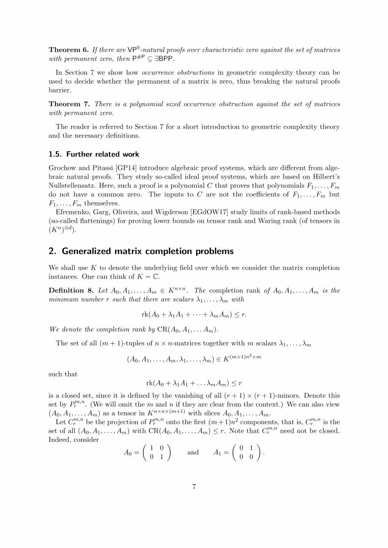
In Section 7 we show how occurrence obstructions in geometric complexity theory can beused to decide whether the permanent of a matrix is zero, thus breaking the natural proofsbarrier.

Theorem 7. There is a polynomial sized occurrence obstruction against the set of matriceswith permanent zero.

The reader is referred to Section 7 for a short introduction to geometric complexity theoryand the necessary definitions.

1.5. Further related work

Grochow and Pitassi [GP14] introduce algebraic proof systems, which are different from alge-braic natural proofs. They study so-called ideal proof systems, which are based on Hilbert’sNullstellensatz. Here, such a proof is a polynomial C that proves that polynomials F1, . . . , Fmdo not have a common zero. The inputs to C are not the coefficients of F1, . . . , Fm butF1, . . . , Fm themselves.

Efremenko, Garg, Oliveira, and Wigderson [EGdOW17] study limits of rank-based methods(so-called flattenings) for proving lower bounds on tensor rank and Waring rank (of tensors in(Kn)⊗d).

2. Generalized matrix completion problems

We shall use K to denote the underlying field over which we consider the matrix completioninstances. One can think of K = C.

Definition 8. Let A0, A1, . . . , Am ∈ Kn×n. The completion rank of A0, A1, . . . , Am is theminimum number r such that there are scalars λ1, . . . , λm with

rk(A0 + λ1A1 + · · ·+ λmAm) ≤ r.

We denote the completion rank by CR(A0, A1, . . . Am).

The set of all (m+ 1)-tuples of n× n-matrices together with m scalars λ1, . . . , λm

(A0, A1, . . . , Am, λ1, . . . , λm) ∈ K(m+1)n2+m

such thatrk(A0 + λ1A1 + . . . λmAm) ≤ r

is a closed set, since it is defined by the vanishing of all (r + 1)× (r + 1)-minors. Denote thisset by Pm,nr . (We will omit the m and n if they are clear from the context.) We can also view(A0, A1, . . . , Am) as a tensor in Kn×n×(m+1) with slices A0, A1, . . . , Am.

Let Cm,nr be the projection of Pm,nr onto the first (m+1)n2 components, that is, Cm,nr is theset of all (A0, A1, . . . , Am) with CR(A0, A1, . . . , Am) ≤ r. Note that Cm,nr need not be closed.Indeed, consider

A0 =

(1 00 1

)and A1 =

(0 10 0

).

7

Clearly, CR(A0, A1) = 2. But we have(1 0ε 1

)︸ ︷︷ ︸

=:A0,ε

+1

ε

(0 10 0

)=

(1 1/εε 1

).

(Think of ε being a small number for the moment.) Thus, we have CR(A0,ε, A1) = 1 for everyε 6= 0. Then (A0,ε, A1) converges to (A0, A1) in the Euclidean topology. Hence (A0, A1) hascompletion rank 2 but is contained in the Euclidean (and also Zariski) closure of C1.

In our definition of border completion rank, an important question is: with respect to whichambient variety shall we take the Zariski closure? Let B be any rank-one matrix. Then thecompletion rank of (I,B) is at least n − 1. Here, I is the n × n identity matrix. We canapproximate B by B + εI. But I − 1

ε (B + εI) has rank 1 and in fact, this trick always works.Therefore, it seems reasonable that the rank of the approximating matrices should be the sameas the matrix itself, so we take the closure in Kn×n×Kn×n

r1 ×· · ·×Kn×nrm , where Kn×n

ρ denotesthe closed set of matrices of rank at most ρ and ri = rk(Ai).

In the following, we give an algebraic definition of border completion rank, as was done forthe tensor rank, see [BCS97]. This has the advantage that it is independent of the underlyingfield. One can also give a definition in terms of limits; over C, these two notions coincide. Inthe following, let ε denote some indeterminate. We will now consider our tensors over the fieldK(ε) of rational functions. For f, g ∈ K(ε), we write f = g +O(εi) if the coefficients of f andg agree for powers εj with j < i when expanded as formal Laurent series (around 0). We writeA = B + O(εi) for two matrices A and B with entries from K(ε), when the same is true inevery component.

Definition 9. Let A0, A1, . . . , Am ∈ Kn×n. The border completion rank of A0, A1, . . . , Am isthe minimum number r such that there are approximations Ai ∈ K(ε)n×nrk(Ai)

with Ai = Ai+O(ε),

0 ≤ i ≤ m, and rational functions λ1, . . . , λm ∈ K(ε) with

rk(A0 + λ1A1 + · · ·+ λmAm) ≤ r.

We denote the border completion rank by CR(A0, A1, . . . Am).

See Section B for a discussion of alternative ways to define the closure and border completionranks.

3. Border completion rank and natural proofs

Let φ be a formula in 2-CNF over the variables x1, . . . , xt with clauses c1, . . . , cs. We want touse NP-hardness of the Max-2-SAT problem to prove that both completion rank and bordercompletion rank are NP-hard. More specifically, the following problem Max-2-SAT is NP-hard,see [ACG+99]: Given a formula φ in 2-CNF and a bound b ∈ Z+, decide whether there is anassignment to the variables of φ that satisfies at least b clauses of φ.

We will define an instance of border matrix completion of size n = 2s and m = t. Ourmatrices will have a block structure, there will be s blocks of size 2× 2, one for each clause.

In the actual construction, the clause gadgets will be on the diagonal of some larger blockdiagonal matrix. The constants will appear in the 0th layer of the tensor that we constructand the coefficients of the ith variable will appear in the ith layer.

8

Let ci = L1 ∨ L2 be a clause in φ. The corresponding clause gadget looks like(1− `1 1

0 1− `2

).

Here `j in the matrix is xk if the literal Lj = xk and it is 1 − xk if Lj = ¬xk, j = 1, 2. Allthese clause gadgets are blocks of our desired block diagonal matrix. More specifically, takethese s clause gadgets as above, one for each clause, and form a block diagonal matrix of it.We get a matrix with affine linear forms as entries. Write this matrix as A0 + x1A1 + . . . xtAt.(A0, A1, . . . , At) is our matrix completion instance.

Observation 10. The clause gadget has rank 1 iff at least one of the literals `1, `2 is set to be1. Otherwise, it has rank 2.

By using the above observations, the following lemma follows immediately.

Lemma 11. CR(A0, A1, . . . , At) ≤ 2s− b iff b clauses of φ can be satisfied. Thus the problem

CR(A0, A1, . . . , At)?≤ k is NP-hard.

Now our goal is to prove Lemma 11 for CR also. Since all variables appear only on thediagonals of the gadgets and only one variable in each entry, we observe:

Observation 12. If i ≥ 1, then each Ai is a diagonal matrix with diagonal entries being ±1.Moreover, if the jth diagonal entry of Ai is non-zero then the jth diagonal entry of any otherAk is zero, for i, k ≥ 1.

Let A0, A1, . . . , At be approximations to A0, A1, . . . , At, that is, Ai = Ai +O(ε).

Lemma 13. There are (invertible) matrices S = In + O(ε) and T = In + O(ε) such thatS · (A0 + λ1A1 + · · ·+ λtAt) · T = A0 + λ1A1 + · · ·+ λtAt for some A0 = A0 +O(ε).

Proof. We first show the existence of S1, T1 of the form In +O(ε) such that S1A1T1 = A1. Letj1, . . . , jp be the indices such that the positions (j1, j1), . . . , (jp, jp) contain exactly the ±1’sof A1. Using elementary row and column operations, we can achieve that A1 agrees with A1

in all columns and rows j1, . . . , jp. Note that these elementary and column operations are offollowing two forms.

1. Dividing a row from rows j1, . . . , jp by some constant of the form 1 +O(ε).

2. Adding an O(ε) multiple of some kth row or column to some other row or column, wherek ∈ {j1, . . . , jp}.

Each of the above operations corresponds to left or right multiplying by a matrix of the formIn +O(ε). Thus there exist matrices S1 and T1 of the form In +O(ε), such that S1A1T1 = B1,where B1 agrees with A1 in all columns and rows j1, . . . , jp. Since S1, T1 are of full rank, weget rkA1 = rk A1, thus B1 cannot have any nonzero entries outside these rows j1, . . . , jp andcolumns j1, . . . , jp. Therefore, S1A1T1 = B1 = A1.

Similarly, we obtain S2, T2 of the form In + O(ε) such that SA2T = A2. By observingthe form of elementary and column operations in S2 and T2 as above and also using theobservation above that non-zero diagonal entries of A1 and A2 occur at distinct indices, we getthat S2A1T2 = A1. Now we can continue this process of converting Ai to Ai as well. Thus wemay assume that the approximation Ai are replaced by the exact matrices Ai. This processchanges A0 to some other approximation of A0, which we called A0 in the statement of thelemma.

9

Since S and T above have full rank, we get that rk(A0+λ1A1+ · · ·+λtAt) = rk ˆ(A0+λ1A1+· · · + λtAt). Thus to prove the NP-hardness of border completion rank, we can assume thatAi = Ai for i ≥ 1. We rename A0 back to A0. Assume there are λi = ai,0ε

di + ai,1εdi+1 + . . .

with ai,0 6= 0 such thatrk(A0 + λ1A1 + · · ·+ λtAt) ≤ 2s− b. (1)

Here, di can be any integer, not necessarily non-negative.

Lemma 14. CR(A0, A1, . . . , At) ≤ 2s− b iff b clauses of φ can be satisfied.

Proof. By Lemma 11, we know that if b clauses of φ can be satisfied then CR(A0, A1, . . . , At) ≤2s− b, thus CR(A0, A1, . . . , At) ≤ CR(A0, A1, . . . , At) ≤ 2s− b.

Now we show that if CR(A0, A1, . . . , At) ≤ 2s− b then b clauses of φ can be satisfied. Thismeans that there exist λi as in (1).

If all di ≥ 0, then we can substitute ε = 0 in (1) to get rk(A0 + λ1A1 + · · ·+ λtAt) ≤ 2s− b,thus CR(A0, A1, . . . , At) ≤ 2s − b. By again using Lemma 11, we obtain that b clauses of φcan be satisfied. Thus we can assume w.l.o.g. that some dk < 0. Note that the λi induce anassignment to the xi and thus to literals `j ’s in the clauses, although this assignment mightnot be Boolean and might have negative powers of ε. A clause gadget of clause ci = L1 ∨ L2

in A0 + λ1A1 + · · ·+ λtAt looks like(1 +O(ε)− `1 1 +O(ε)

O(ε) 1 +O(ε)− `2

)For the above clause gadget to have rank one, we need to have `1 = 1+O(ε) or `2 = 1+O(ε).

We call such clauses to be “ε-satisfied” which satisfy `1 = 1 +O(ε) or `2 = 1 +O(ε). Supposewe have at least b “ε-satisfied” clauses. By substituting ε = 0 in corresponding λi’s, we get anassignment of corresponding xi’s. The rest of the xi’s are assigned arbitrary 0 or 1 values. Itis clear that this assignment of xi’s satisfies all the clauses which were “ε-satisfied”, thus theexistence of b “ε-satisfied” clauses implies that b clauses of φ can be satisfied.

Therefore we can assume that there are less than b “ε-satisfied” clauses. We shall use thisassumption to prove that rk(A0 + λ1A1 + · · ·+ λtAt) > 2s− b. For this, we shall construct anon-vanishing minor M of size at least 2s− b+ 1.

We take both rows and columns of clause gadgets for which the corresponding clause is not“ε-satisfied”. For the clause gadgets whose clause is “ε-satisfied”, we take the first row andsecond column, this entry is of the form 1+O(ε). This completes the construction of M . Sincethere are less than b “ε-satisfied” clauses, size of the M is > 2s− b. Let us use k to denote thesize of M , so we have k > 2s− b.

Now we show thatM does not vanish. IfM = (mi,j) then det(M) =∑

σ∈Sk sign(σ)∏i∈[k]mi,σ(i).

By construction, the elements on the diagonal of M have the unique power of ε of minimumdegree in their respective row, when the corresponding clause is “ε-satisfied”. In the casewhen a clause is not “ε-satisfied”, then the entries in the corresponding 2 × 2-block have theminimum degree in the two corresponding rows. However, since the lower-left entry is of theform O(ε), again, only the elements on the diagonal can contribute to the minimum degreemonomial of det(M). Thus, this power of ε cannot be canceled by any other term in the sum∑

σ∈Sk sign(σ)∏i∈[k]mi,σ(i). Therefore det(M) 6= 0. Hence rk(A0+λ1A1+ · · ·+λtAt) > 2s−b,

a contradiction.

Proof of Theorem 3. This follows immediately from Lemma 14 and the NP-hardness of Max-2-SAT.

10

Let t ∈ Km×n×(m+1) be a tensor. Recall that an algebraic poly(n)-natural proof for theborder completion rank of t being > r is a polynomial equation p ∈ K[Xh,i,j |1 ≤ i, j ≤ n, 1 ≤j ≤ m] such that

1. p(t) 6= 0,

2. p(s) = 0 for every s ∈ Kn×n×(m+1) with CR(s) ≤ r.

3. p is computed by a constant-free algebraic circuit of size poly(n).

We here confine ourselves to constant-free circuits. Over fields of characteristic 0, we candeal with arbitrary constants similar to [GP14], at the price of replacing ∃BPP by BP-NP.Note that our proofs have an additional condition (compared to Forbes et al. [FSV17]) that itshall not vanish on a certain tensor t. So we want a concrete proof for some tensor t. (Notehowever, that if p(t) 6= 0, then p proves this for a lot of tensors, since the set at which p doesnot vanish is open.) Forbes et al. only demand that p is nonzero, that is, that it can prove alower bound for some unknown tensor (and henceforth for many unknown tensors).

Observation 15. Let Ui,j , Vi,j, 1 ≤ i ≤ ρ, 1 ≤ j ≤ n be indeterminates over K. Consider thepolynomial matrix

ρ∑i=1

(Ui,1, . . . , Ui,n)T (Vi,1, . . . , Vi,n).

If we substitute arbitrary constants for the indeterminates, then we get all matrices in Kn×nρ

Lemma 16. Let Q0, Q1, . . . , Qt be polynomial matrices as in Observation 15, having ranksr0, . . . , rt, respectively. We use fresh variables for each Qi. Let g := (Q0 − Z0Q1 − · · · −ZtQt, Q1, . . . , Qt), where Z1, . . . , Zt are new variables. If we substitute arbitrary constants forthe indeterminates, then we get all tensors of completion rank ≤ r0 with the ith slice havingrank ≤ ri, 1 ≤ i ≤ t.

Proof. By Observation 15, the images of each Qi give all of the matrices of rank ri. If a tensor(A0, A1, . . . , At) has completion rank at most r0, then then there are scalars λ1, . . . , λt suchthat A0 + λ1A1 + · · ·+ λtAt has rank ≤ r0. This means that there is a rank r0 matrix B suchthat A0 = B − λ1A1 − · · · − λtAt. This is exactly generated in the first component of g.

Proof of Theorem 4. The tensors will be the tensors constructed above from 2-CNF formulas.Assume that the assertion of the theorem is false and let n be large enough such that for alltensors under consideration, there is a algebraic poly(n)-natural proof.

Let φ be a formula in 2-CNF and let b ∈ N. We want to check whether every assignment sat-isfies < b clauses of φ. This problem is coNP-hard. Let Tφ = (A0, . . . , At) be the correspondingtensor constructed above in Theorem 3. Let p be a polynomial that vanishes on all tensorsof border completion rank ≤ 2s − b but not on Tφ and that has polynomial-size arithmeticcircuits. Such a polynomial is guaranteed to exist by assumption. However, we do not knowhow to construct such a p.

We can use the nondeterminism to guess a polynomial-sized circuit. Then we have to verifythat the polynomial p computed by the circuit has indeed this property.

Let g be the tensor of Lemma 16 with r0 = 2s− b and ri = rk(Ai), 1 ≤ i ≤ t. If p(g) = 0 asa polynomial identity, then by Lemma 16, p vanishes on all tensors of completion rank r0 thathave ranks of the slices 1, . . . , t bounded by r1, . . . , rt. Since p is a polynomial, it also vanishes

11

on all tensors of border completion rank r0 that have ranks of the slices 1, . . . , t bounded byr1, . . . , rt.

Now given Tφ, we can decide whether b clauses of φ cannot be satisfied, as follows:

1. Guess a circuit C of polynomial size computing a polynomial p.

2. Decide whether p(g) = 0 using polynomial identity testing.

3. Check whether p(Tφ) 6= 0. If yes, then accept. Otherwise reject.

The correctness follows from the construction. It is obviously an ∃BPP algorithm. Note thatp(Tφ) 6= 0 can again be checked by polynomial identity testing. (A direct evaluation might notbe possible, since this could involve large numbers.)

Note that the nonexistence of algebraic poly(n)-natural proofs does not simply follow fromthe NP-hardness of border completion rank. It could have been the case that all the proofshave polynomial size, but they cannot be constructed in polynomial time. Or there could bemany such proofs, because the variety has many components.

Observation 17. In the hardness proof for border completion rank, we look at tensors (A0, A1, . . . , At)of border completion rank at most r with rk(Ai) ≤ c for all i for some constant c and eachAi has size n := 2s. The variety Cn,t,cr of all such tensors is irreducible: We can think ofg constructed in Lemma 16 as a polynomial map from Kn×r × Kr×n × (Kn×c × Kc×n)t toKn×n×t. The closure of the image of g is Cn,t,cr . Therefore, Cn,t,cr itself is irreducible.

We can strengthen the statement of Theorem 4: There are infinite sequences tn = Θ(n) andrn = Θ(n) and a constant c such that for every set of equations describing the variety Cn,tn,crn ,at least one equation has superpolynomial circuit complexity, unless coNP ⊆ ∃BPP.

4. Relation to (border) tensor rank

The following theorem was essentially shown by Derksen [Der14]. The proof uses the well-known fact that if a slice of a tensor t has rank-one, then we can use this slice in an optimaldecomposition of t into rank-one tensors.

Theorem 18. If t = (A0, A1, . . . , Am) is tensor such that the slices A0, A1, . . . , Am are linearlyindependent and rk(A1) = · · · = rk(Am) = 1, then

R(t) = CR(t) +m.

It is not clear whether the same is true for border rank and border completion rank. Wecan prove that the right-hand side is an upper bound for the left-hand side.

Proposition 19. If t = (A0, A1, . . . , Am) is a tensor such that rk(A1) = · · · = rk(Am) = 1.Then

R(t) ≤ CR(t) +m.

Proof. Let r = CR(t) and let (A0, A1, . . . , Am) be approximations to (A0, A1, . . . , At) withrk(Ai) = rk(Ai) = 1 for 1 ≤ i ≤ m and λ1, . . . , λm ∈ K(ε) such that

rk(A0 + λ1A1 + · · ·+ λmAm) ≤ r.

12

We can write each Ai = ui ⊗ vi with ui, vi ∈ K[ε]n. Since rk(A0 + λ1A1 + · · · + λmAm) ≤ r,there are vectors x1, . . . , xr, y1, . . . , yr ∈ K(ε) such that

A0 + λ1A1 + · · ·+ λmAm = x1 ⊗ y1 + · · ·+ xr ⊗ yr.

Therefore,

t = e0 ⊗ x1 ⊗ y1 + · · ·+ e0 ⊗ xr ⊗ yr+ (−λ1e0 + e1)⊗ u1 ⊗ v1 + · · ·+ (−λme0 + em)⊗ um ⊗ vm+O(ε),

where e0, . . . , em denotes the standard basis (corresponding to the slices). Therefore, R(t) ≤r +m.

Can we prove an analogue of Theorem 4 for the border rank? First of all, we do not knowwhether a converse of Theorem 18 is true. More severe, however, seems to be the restriction tomatrices of rank 1. In the next Section 5, we will introduce clause gadgets that only containrank-one matrices. But they only work for the tensor rank, not for the border tensor rank,since they allow solutions in the border that do not correspond to Boolean assignments. Bordercompletion rank is more forgiving; there we could use more compact gadgets, that did not allowunwanted solutions in the border, because there were no rank restrictions.

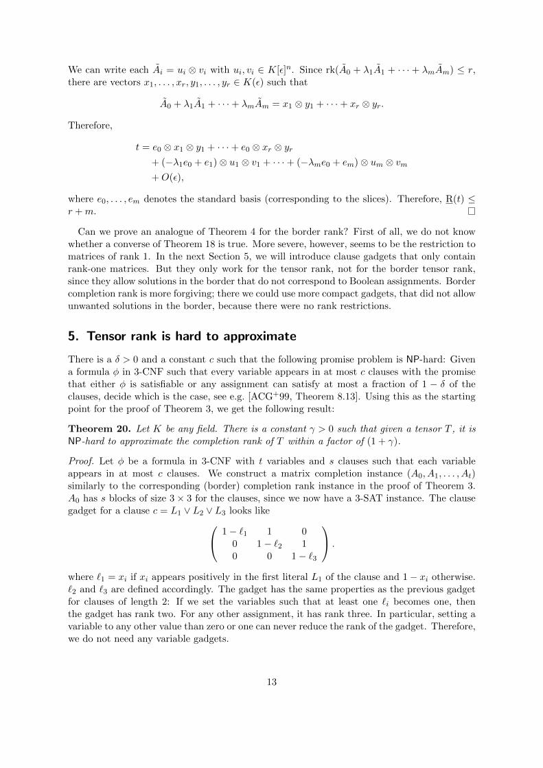
5. Tensor rank is hard to approximate

There is a δ > 0 and a constant c such that the following promise problem is NP-hard: Givena formula φ in 3-CNF such that every variable appears in at most c clauses with the promisethat either φ is satisfiable or any assignment can satisfy at most a fraction of 1 − δ of theclauses, decide which is the case, see e.g. [ACG+99, Theorem 8.13]. Using this as the startingpoint for the proof of Theorem 3, we get the following result:

Theorem 20. Let K be any field. There is a constant γ > 0 such that given a tensor T , it isNP-hard to approximate the completion rank of T within a factor of (1 + γ).

Proof. Let φ be a formula in 3-CNF with t variables and s clauses such that each variableappears in at most c clauses. We construct a matrix completion instance (A0, A1, . . . , At)similarly to the corresponding (border) completion rank instance in the proof of Theorem 3.A0 has s blocks of size 3× 3 for the clauses, since we now have a 3-SAT instance. The clausegadget for a clause c = L1 ∨ L2 ∨ L3 looks like 1− `1 1 0

0 1− `2 10 0 1− `3

.

where `1 = xi if xi appears positively in the first literal L1 of the clause and 1− xi otherwise.`2 and `3 are defined accordingly. The gadget has the same properties as the previous gadgetfor clauses of length 2: If we set the variables such that at least one `i becomes one, thenthe gadget has rank two. For any other assignment, it has rank three. In particular, setting avariable to any other value than zero or one can never reduce the rank of the gadget. Therefore,we do not need any variable gadgets.

13

If φ is satisfiable, then CR(A0, A1, . . . , At) = 2s; this rank is achieved by any satisfyingassignment to φ.

Now assume that φ is not satisfiable, then any assignment to the variables can satisfy atmost (1 − δ)s clauses. Since we are only considering completion rank, the situation is mucheasier compared to border completion rank: A0 +λ1A1 + · · ·+λtAt is a block diagonal matrix.The rank of A0 + λ1A1 + · · · + λtAt is 2s + u where u is the number of clause gadgets thathave rank three. From λ1, . . . , λt, we construct a Boolean assignment by setting xi to λi ifλi ∈ {0, 1} and to an arbitrary Boolean value otherwise. This Boolean assignment satisfies atleast s−u clauses. Since φ is not satisfiable, u ≥ δs. Therefore, CR(A0, A1, . . . , At) ≥ (2+δ)s.

Therefore, the reduction is approximation preserving and we obtain the statement of thetheorem.

Next, we want to use this construction to show that also tensor rank is hard to approximate.The idea is to go via Theorem 18. To this aim, we have to ensure that every matrix A1, . . . , Athas rank 1. Our construction is inspired by the work of Schaefer and Stefankovic [SS16], butit is tailored to formulas in 3-CNFs and therefore it is easier to analyze, in particular whenproving approximation hardness.

Assume we have a clause with variables x, y and z. The clause gadget looks as follows:

1 x 0 0 0 0 0 0 01 u 0 0 0 0 s(u)− u1 0 00 0 1 y 0 0 0 0 00 0 1 v 0 0 0 s(v)− v1 00 0 0 0 1 z 0 0 00 0 0 0 1 w 0 0 s(w)− w1

0 u− u2 0 0 0 0 1− `(u) 1 00 0 0 v − v2 0 0 0 1− `(v) 10 0 0 0 0 w − w2 0 0 1− `(w)

.

We have

`(u) =

{u if x appears positively in the clause,

1− u otherwise,

and

s(u) =

{−u if x appears positively in the clause,

u otherwise.

`(v), s(v), `(w), and s(w) are defined accordingly.All matrices have rank one. The gadget consists of three 2× 2-blocks on the diagonal which

create local variables u, v, and z, which are copies of x, y, and z. The 3× 3-block in the lowerright corner implements the clause. All other entries not in these blocks are only introducedto make the matrices rank 1.

The variables u, v, and w are local variables that are only used within the gadget. Thevariables ui, vi, and wi are also local variables, they are needed to make all occurring matricesrank one: For instance, the local variable u appears on the diagonal twice, locally in positions(2, 2) and (7, 7). To make the corresponding 2× 2-submatrix rank one, we add the variable uto the two other corners (2, 7) and (7, 2) of this 2 × 2-submatrix. The entry position (7, 7) iseither u or −u. In order to get a rank one matrix, the entry in position (2, 7) will also be u or

14

−u, respectively. To be able to recover the original diagonal submatrix, we also add new localvariables u1 and u2 in the positions (2, 7) and (7, 2). The same is done for the variables v andw.

The variables x, y and z (and all further variables of the formula, of course), appear inseveral clause gadgets. Therefore, the matrix that corresponds to say x does not have rankone. We use the same construction as for the local variables in the overall construction, whichis described after the next lemma.

Lemma 21. 1. If we set x, y, z to values from {0, 1} such that the clause is satisfied, thenthe local variables in the clause gadget can be set such that the resulting matrix has rankfive.

2. If the variables are set in such a way that the rank of the clause gadget is five, then x, y, zare set such that the clause is satisfied, which means that at least one variable is set to avalue from {0, 1} and this value satisfies the corresponding literal.

Proof. For the first item, we construct an assignment for the local variables as follows: weset u = x, v = y, and w = z and all variables ui, vi, and wi in such a way that the uniqueentry they appear in becomes zero. In this way, we are left with a block diagonal matrix. Inthe three 2 × 2 blocks, the second row equals the first row or is zero. The 3 × 3-block is theoriginal clause gadget. Since the assignment satisfies the clause, the rank of this block is two.Therefore, the overall rank is five.

For the second item, we will derive several equations from the fact that the rank of thegadget is five. Consider the clause gadget with rows 4,6,9 and columns 4,6,7 removed:

1 x 0 0 0 01 u 0 0 0 00 0 1 0 0 00 0 0 1 0 00 u− u2 0 0 1 00 0 0 0 1− `(v) 1

.

Its determinant is u−x. Next consider the gadget with rows 2,6,9 and columns 2,6,7 removed:

1 0 0 0 0 00 1 y 0 0 00 1 v 0 s(v)− v1 00 0 0 1 0 00 0 0 0 1 00 0 v − v2 0 1− `(v) 1

.

Its determinant is v − y. Next comes the gadget with rows 2,4,9 and columns 2,4,7 removed:

1 0 0 0 0 00 1 0 0 0 00 0 1 z 0 00 0 1 w 0 s(w)− w1

0 0 0 0 1 00 0 0 0 1− `(v) 1

.

15

The determinant is w − z. Finally consider the gadget with rows and columns 2,4,6 removed:

1 0 0 0 0 00 1 0 0 0 00 0 1 0 0 00 0 0 1− `(u) 1 00 0 0 0 1− `(v) 10 0 0 0 0 1− `(w)

.

Its determinant is (1− `(u))(1− `(v))(1− `(w)).Assume that we have an assignment such that the clause gadget has rank 5. Then the

vanishing of the first three minors enforces that x = u, y = v, and z = w and the vanishing ofthe last one that at least one literal is one and hence the clause is satisfied (and therefore atleast one of x, y or z is from {0, 1}).

Let φ be a formula in 3-CNF with t variables and s clauses such that every variable appearsin a constant number c of clauses. Note that s = O(t). In our final construction, for everyclause, we will have one clause gadget. These gadgets are arranged as a block diagonal matrix.The matrices that correspond to an actual variable of φ are not rank-one matrices. We makethem rank-one as we did locally in the clause gadgets, as described above: If x appears inpositions (i1, j1), . . . , (ik, jk), then we replace this matrix by a rank one matrix with 1’s in allpositions (ih, j`), 1 ≤ h, ` ≤ k. k is at most c, since each variable appears in at most c clauses.For all tuples (ih, j`) with h 6= `, we have an additional rank-one matrix with a 1 in thisposition and 0s elsewhere, corresponding to a new variable xh,` in the completion problem. Inthis way, the original diagonal matrix is in the span of these matrices. Let Tφ be the resultingtensor. By construction, all slices have rank 1 except for the 0th slice. The number of slicesof Tφ is O(t), since each clause gadget introduces a constant number of slices. Furthermore,there are only a constant number, namely ≤ c2, of additional rank-one matrices introduced inthe last step.

Lemma 22. Assume that φ is either satisfiable or any assignment satisfies at most (1− ε) ofthe clauses for some ε > 0.

1. If φ is satisfiable, then the completion rank of Tφ is at most 5s.

2. If φ is not satisfiable, then the completion rank of Tφ is at least 5s+ εs.

Proof. If φ is satisfiable, then we set each variable in Tφ corresponding to an original variableof φ to the value of a satisfying assignment. By Lemma 21, we can set all clause gadgetslocally such that their rank is 5. We set the auxiliary variables xh,` in such a way that we clearall elements not in a block on the diagonal. Therefore, the completion rank is at most 5s.

For the second item, assume that the completion rank of Tφ is r < 5s + εs. Choose anassignment to the variables of Tφ that achieves this completion rank. Choose linear independentcolumns a1, . . . , ar of the resulting matrix A.

From every clause gadget, the local columns 1, 3, 5, 8, and 9 are linearly independent, evenif we remove the local rows 1, 3, and 5. In the overall construction, there are only nonzeroentries outside the gadget in the local columns 2, 4, and 6 and rows 1, 3, and 5. Therefore, wecan always assume that for any clause gadget, its local columns 1, 3, 5, 8, and 9 are amongthe a1, . . . , ar.

16

Now consider a gadget G that contributes more than five columns to a1, . . . , ar. There areat most εs such gadgets. Assume that the local column 2 of G is among a1, . . . , ar and it isai. Furthermore, let the variable in ai be x. Then we can use the variables xh,j to clear allentries in the column ai outside the gadget. This will not affect the other columns of A, sinceevery column has its own variables. If thereafter, ai is in the span of the remaining columns,then we can exchange it against a new column from A, since r was the completion rank of Tφ.By repeating this process if necessary, we can assume that no ai has nonzero entries outsidethe clause gadgets, since the same reasoning works for the local columns 4 and 6 and the localcolumn 7 has no nonzero entries outside the gadget by construction. Therefore, we can assumew.l.o.g. that A is a block diagonal matrix and the blocks on the diagonal are instantiations ofthe clause gadgets.

Now we have clause gadgets with five columns among the a1, . . . , ar and clause gadgets withsix or more. We claim that the assignment to the variables of Tφ that correspond to variablesof φ is an assignment that satisfies all clauses with only five columns among a1, . . . , ar. If thisis the case, then we get a satisfying assignment which satisfies a fraction of more than (1− ε)of all clauses and henceforth, φ is satisfiable.

Let G be a clause gadget with only five columns among a1, . . . , ar. Choose r − 5 rows fromthe other clause gadgets to get an invertible (r − 5) × (r − 5)-submatrix M of A, which isdisjoint from G. Choose a 6 × 6-submatrix S of G. As a submatrix of A, S and M form ablock diagonal matrix. The determinant of this matrix vanishes, since its size is (r+1)×(r+1),but r is the completion rank. Since M is invertible, it follows that all 6×6 minors of G vanish.By Lemma 21, the assignment satisfies the corresponding clause.

The inapproximability of tensor rank follows immediately from the lemma above togetherwith Theorem 18.

Theorem 23. Tensor rank is NP-hard to approximate.

Proof. Let Tφ be the tensor in Lemma 22. By Theorem 18, R(Tφ) = CR(Tφ)+k where k is thetotal number of slices of Tφ. Since every variable of φ occurs only a constant number of timesin φ and every gadget has constant size, k = Θ(t). Since CR(Tφ) is hard to approximate, so isR(Tφ).

6. Matrices with permanent zero and a transfer theorem

In this section we prove Theorem 5 and 6. When Grochow and Pitassi [GP14] studied so-calledideal proof systems, they used their framework to provide a short proof of a transfer theorem,namely that VP0 = VNP0 implies that coNP ⊆ ∃BPP. Such a transfer theorem shows thatseparations in the Boolean world yield separations in the algebraic world. (We do not know ofany transfer theorem in the other direction.) One could use our framework to do somethingsimilar; however, with roughly the same effort, we can prove an even stronger transfer theorem.The starting point is algebraic VP0-natural proofs for the set of all matrices A, say with rationalentries, that fulfill Per(A) = 0. (Note that we allow negative entries.) Note that this set hasa VNP0-natural proof, namely the permanent itself. We will prove that if there is a family ofpolynomials (Dn) ∈ VP0 such that Dn is nonzero and vanishes on all matrices with permanent0, then we can construct a circuit for the permanent in ∃BPP. This uses the self-reducibility ofthe permanent, similar to [KI04], and Kaltofen’s factorization algorithm [Kal89]. In particular,if VP0 = VNP0, then this will allow us to show that P#P ⊆ ∃BPP.

17

Let X be an n× n matrix. Construct an n× n matrix Z as follows:zij = xij for i ≤ n− 1,

znj = xnj PerXnn for j ≤ n− 1,

znn = −∑n−1

j=1 xnj PerXnj ,

where Xij is the matrix obtained from X by removing the ith row and the jth column. Wehave PerZ = 0. Moreover, any matrix with PerZ = 0 and PerZnn 6= 0 can be obtained in thisway, by Laplace expansion. The following theorem from [Kal89] states that if a polynomialcan be computed by small circuit then so can be its factors. We only need this result for primefields, so we state it only for prime fields Fp.

Theorem 24 (Kaltofen [Kal89]). If f ∈ Fp[x1, . . . , xn] can be computed by an arithmetic

circuit of size at most s and degree at most d, f =∏ki=1 g

pei ·jii , where the gi’s are irreducible

and p - ji for each i. Then we can compute, for each i ∈ [k], the numbers ei, ji, and anarithmetic circuit for the factor gp

ei

i in randomized poly(n, s, d, log p) time.

Although Theorem 24 works for the factors of the form gpei

i , in our special case ei wouldalways be zero, thus giving us the factor gi directly. We also need the following lemma from[FPdV13], which bounds the size of coefficients of any VP0 polynomial.

Lemma 25 (Fournier-Perifel-Verclos [FPdV13]). Let P be a polynomial computed by an arith-metic circuit of size s and formal degree d with constants of absolute value bounded by M ≥ 2,then the sum of the absolute values of its coefficients is at most M s·d.

Now we are ready to prove our result.

Proof of Theorem 5. If VP0 = VNP0, there exists a VP0-family of circuits computing Pern. Lets(n) be a polynomial bound on the size of a circuit for Pern and d(n), on its formal degree.

We describe an ∃BPP algorithm which computes a circuit for Pern over Fp[x1,1, . . . , xn,n] forsome p > n!. These circuits can be used to implement any language from P#P.

The algorithm uses non-determinism to guess a circuit for Perk for each k ≤ n. We startfrom the trivial circuit for Per1. For each k, perform the following steps:

1. Use non-determinism to guess a VP0-circuit Ck of size ≤ s(k), which potentially computesPerk.

2. Check that its formal degree is ≤ d(k), otherwise reject.

3. Use a randomized algorithm for PIT to check that Ck(Zk(X)) = 0, otherwise reject.Here Zk(X) denotes the matrix constructed above of size k × k with entries taken fromX = (xi,j). Note that the parameterization Zk uses Perk−1, which can be computed bythe circuit for Perk−1 obtained on the previous iteration. Here we make sure that thisPIT succeeds with probability at least 1− 1

3n2 .

4. By Hilbert’s Nullstellensatz, the polynomial computed by Ck has the form (Perk)eh with

e ≤ d(k)k and gcd((Perk)

e, h) = 1. Note that Perk is irreducible.

5. Since Ck has a VP0-circuit of size s(k) and formal degree d(k), we know that the magni-tude of coefficients of Ck is bounded by B := 2d(k)·s(k), this follows from Lemma 25. Sowe choose a prime p > max{B,n!}. By the choice of p, we see that Ck = (Perk)

eh evenover Fp[x1,1, . . . xk,k].

18

6. Now we use Theorem 24 to obtain a circuit for all the irreducible factors gi of Ck =∏ki=1 g

pei ·jii in randomized poly(n, s(k), d(k), log p) = poly(n, s(k), d(k)) time. Since we

choose p to be large enough, we know that all ei = 0 and p - ji for all i. Here also, weassume that this randomized algorithm succeeds with probability at least 1− 1

3n2 .

7. For all irreducible factors gi’s of Ck, use a randomized algorithm for PIT to check thatgi(Zk(X)) = 0. Here we make sure that this PIT succeeds with probability at least1 − 1

3·d(k)·n2 . If this PIT succeeds then we know that gi has to be Perk since gi is

irreducible. Thus we can compute a constant free circuit for Perk with probability 1− 1n2 ,

of size poly(n, s(k), d(k)).2

Since we have n iterations, overall success probability is at least 1− 1n . Thus P#P ⊆ ∃BPP.

A slight modification of the proof of Theorem 5 gives a proof of Theorem 6 as follows.

Proof of Theorem 6. Let the set of permanent zero matrices have VP0-natural proofs. Thenthere exists a family (Dk)k∈N ∈ VP0 of nonzero polynomials such that Dk vanishes on k × kmatrices of permanent zero. Let s(k) be the size of Dk and d(k) be its formal degree. Bothare polynomially bounded by definition of VP0.

We proceed precisely as in the proof of Theorem 5. Note that in this proof, we only neededthe fact that Perk has small circuits to have an upper bound on the size of the guessed circuitCk that computes a polynomial that vanishes on all k× k-matrices. Here this bound is simplygiven by Dk.

7. Geometric complexity theory breaks the natural proofs barrier

In this section we show how geometric complexity theory breaks the natural proofs barrierpresented in Theorem 6, see Theorem 7.

Geometric complexity theory is an approach towards algebraic complexity lower boundsvia tools from algebraic geometry and representation theory. In [MS01,MS08] Mulmuley andSohoni define obstructions, which are representation theoretic multiplicities that can be usedto show complexity lower bounds. In this section we discuss how this approach can potentiallybreak the algebraic natural proofs barrier. Indeed, we will show that it breaks the barrier inthe “permanent = 0” example.

Let Z ⊆ Cn×n be the variety of matrices with permanent zero. Theorem 6 shows that ifZ has VP0-natural proofs, then P#P ⊆ ∃BPP. In this section we show that for every pointoutside of Z we can prove that it lies outside of Z by using representation theoretic occurrenceobstructions, analogously to those that were proposed in [MS01, MS08], see the definitionsbelow. Since these occurrence obstructions have a succinct encoding, in the “permanent = 0”setting geometric complexity theory breaks the algebraic natural proof barrier.

For the necessary background on group actions and representation theory of the symmetricgroup, the general linear group, and the algebraic torus we direct the reader to the lecturenotes [BI17], or to the excellent textbooks [Sag01], [Ful97, parts I and II], and [FH91, Ch. 4

2Note that we factor a newly guessed circuit every time. We only need the circuit of the previous round tocheck whether Ck vanishes on Zk(X) but not as a building block of Ck. So we will not have a repeatedincrease in circuit size due to factoring.

19

and Ch. 15]. The group GLn×GLn acts on the set of matrices Cn×n via left-right multiplication:

(g1, g2) ·A := g1A(g2)T ,

for A ∈ Cn×n, (g1, g2) ∈ GLn × GLn, where the transpose is taken for technical reasons3.Let Tn ⊆ GLn denote the algebraic torus (i.e., the group of diagonal matrices with nonzerodeterminant) and let Sn ⊆ GLn denote the symmetric group embedded into GLn via permu-tation matrices. Let Qn ⊆ GLn denote the group of monomial matrices, i.e., matrices withnonzero determinant that have a single nonzero entry in each row and column. As a group Qnis isomorphic to a semi-direct product TnoSn. Since the permanent is invariant (up to scale)under rescaling of rows and columns and permuting rows and columns, the variety Z is closedunder the action of the group G := Qn ×Qn ⊆ GLn ×GLn, which means that if A ∈ Z, thengA ∈ Z for all g ∈ G.

To show that a matrix A does not lie in Z, the geometric complexity approach goes as follows.For the sake of contradiction, assume that A ∈ Z. Then the whole orbit GA := {gA | g ∈ G}is contained in Z, because Z is closed under the action of G. Since Z is also Zariski-closed,we have GA ⊆ Z as a sub-variety. Let C[Cn×n] := C[x1,1, . . . , xn,n] denote the C-algebraof polynomials on the space of n × n-matrices. For a Zariski-closed subset Y ⊆ Cn×n letI(Y ) ⊆ C[Cn×n] denote the vanishing ideal of Y , i.e., the ideal of polynomials that vanishidentically on Y . If Y is invariant under rescaling (which is true for our sets of interest, Y = Zor Y = GA), then the vanishing ideal inherits the grading from the polynomial ring: Wedenote by I(Y )d the homogeneous degree d component of I(Y ). We define the coordinate ringC[Y ] of Y as the quotient C[Y ] := C[Cn×n]/I(Y ), which also naturally inherits the gradingC[Y ]d := C[Cn×n]d/I(Y )d. Since GA ⊆ Z, it follows I(Z)d ⊆ I(GA)d for all d. Therefore therestriction of functions gives a canonical surjection between finite dimensional vector spaces:

C[Z]d � C[GA]d. (2)

Since Z and GA are closed under the action of G, we get an action on the coordinate rings viathe so-called canonical pullback

(gf)(B) := f(gTB)

for g ∈ G, f ∈ C[Y ], B ∈ Cn×n. In this way, both C[Z]d and C[GA]d are G-representations inthe following sense:

For a group H (e.g. H = G, H = Tn, H = GLn, H = Tn × Tn, H = Sn × Sn), anH-representation is a finite dimensional vector space V with a group homomorphism % : H →GL(V ). For an element g ∈ H and a vector f ∈ V we use the shorthand notation gf for(%(g))(f). A linear map ϕ : V1 → V2 between two H-representations V1 and V2 is calledequivariant if for all g ∈ H and f ∈ V1 we have ϕ(gf) = gϕ(f). A bijective equivariant map iscalled an H-isomorphism. Two H-representations are called isomorphic if an H-isomorphismexists from one to the other. A linear subspace of an H-representation that is closed under theaction of H is called a subrepresentation. An H-representation whose only subrepresentationsare itself and 0 is called irreducible.

For many groups H the irreducible representations have a complete classification. In or-der to state Proposition 26, we give now describe a natural index set for all irreducible G-representations. A partition λ of n is a non-increasing list of positive integers that sum up

3The transpose gives g(g′A) = (gg′)A for all pairs g ∈ GLn ×GLn, g′ ∈ GLn ×GLn.

20

to n. To each irreducible representation of G we can assign a type, which is a pair of tu-ples in which each tuple consists of a list of n integers and a partition of n. Two irreducibleG-representations are isomorphic iff they have the same type.

Let (1n) denote the list of n many 1’s. We fix the type ν := (((1n), (n)), ((1n), (n))). Theirreducible G-representation V of type ν is 1-dimensional, V = 〈f〉, where the symmetricgroups act trivially and the tori act by rescaling:(

π,diag(α1, . . . , αn) ; σ, diag(β1, . . . , βn))f = α1 · · ·αnβ1 · · ·βnf.

We will use the classification of irreducible representations for other groups H later in theproof of Proposition 26.

The group G (as well as the other groups that we consider in the proof of Proposition 26) islinearly reductive, which means that every G-representation V decomposes into a direct sumof irreducible representations. This decomposition is not necessarily unique, but for each typeλ the multiplicity multλ(V ) of λ in V is unique, which is the number of summands that havetype λ. The famous Schur’s lemma says for an equivariant map ϕ : V → W , the image ϕ(V )is a G-representation and multiplicities do not increase when applying ϕ:

multλ(V ) ≥ multλ(ϕ(V )).

Recall A ∈ Z. The map in (2) is equivariant and thus

multλ(C[Z]d) ≥ multλ(C[GA]d). (3)

A type λ that violates (3) is called an obstruction. By the above reasoning, the existence ofan obstruction proves A /∈ Z. In other words,

if there is a λ with multλ(C[Z]d) < multλ(C[GA]d), then A /∈ Z. (4)

Proposition 26. Let G be the group G := Qn×Qn. We fix the type ν := (((1n), (n)), ((1n), (n))).We have

• multν(C[Z]n) = 0 and

• multν(C[GA]n) =

{0 if A ∈ Z,1 otherwise.

Proposition 26 says that if A /∈ Z, then this can be shown using (4), which can be thought ofas a succinct presentation of the permanent. Here we are in the special case where one of themultiplicities is zero. These obstructions are called occurrence obstructions in the literature.

Proof. The irreducible representations of GLn are indexed by partitions of length at most nand denoted by {λ}. The irreducible representations of Sn are indexed by partitions of n anddenoted by [λ]. The group GLn × GLn × Sd × Sd is linearly reductive and its irreduciblesare tensor products {λ} ⊗ {µ} ⊗ [ν]⊗ [ξ]. The famous Schur-Weyl duality states that the dthtensor power decomposes as follows as a GLn ×GLn ×Sd ×Sd-representation:⊗d(Cn)⊗

⊗d(Cn) =⊕λ,µ`nd

{λ} ⊗ {µ} ⊗ [λ]⊗ [µ],

21

where λ, µ `n d means that we sum over pairs of partitions of d that each have length atmost n. We have the natural isomorphism⊗d(Cn)⊗

⊗d(Cn) '⊗d(Cn×n).

We symmetrize with respect to Sd to convert tensors into polynomials:

C[Cn×n]d =⊕λ,µ`nd

{λ} ⊗ {µ} ⊗ ([λ]⊗ [µ])Sd

=⊕λ`nd{λ} ⊗ {λ},

where ([λ]⊗ [µ])Sd denotes the Sd-invariant space in [λ]⊗ [µ], which is 1-dimensional iff λ = µ,and 0-dimensional otherwise. The irreducible representations of Tn are indexed by lists of nintegers. Now choose d = n and consider the irreducible Tn × Tn subrepresentation of type((1n), (1n)), where we use Gay’s theorem [Gay76] that the sum of irreducible Tn-representationsof type (1n) in {λ} is isomorphic to [λ] as an Sn-representation, provided λ is a partition ofn: {λ}(1n) = [λ]:

(C[Cn×n]n)((1n),(1n)) =⊕λ`n

[λ]⊗ [λ].

As an Sn × Sn-representation, the trivial subrepresentation (i.e., the representation of type((n), (n))) occurs once in this decomposition. This subrepresentation is 1-dimensional, so as aG-representation we have

W := (C[Cn×n]n)ν = C,multν(C[Cn×n]n) = 1.

But the permanent polynomial lies in W , so W is the line spanned by the permanent. Sincethe permanent vanishes on Z we have multν(I(Z)n) = 1 and thus multν(C[Z]n) = 0. ForA ∈ Z we have GA ⊆ Z, therefore multν(C[GA]n) = 0. For every matrix A that does not liein Z we have that the permanent does not vanish on A, so multν(I(GA)n) = 0 and thereforemultν(C[GA]n) = 1.

Now Theorem 7 immediately follows from Proposition 26. Note that the type ν in theproposition is just an efficient encoding of the permanent. So while it is a short proof, itsverification is hard. But this is to be expected, since the permanent is a hard function.

8. Acknowledgement

We would like to thank the STOC 2018 referees for their detailed and very helpful comments.We would also like to thank Peter Burgisser for enlightening discussions at the Workshop onAlgebraic Complexity Theory (WACT 2018) in Paris.

References

[ACG+99] G. Ausiello, P. Crescenzi, G. Gambosi, V. Kann, A. Marchetti-Spaccamela, andM. Protasi. Complexity and Approximation. Springer, 1999.

22

[AD08] Scott Aaronson and Andrew Drucker. Algebraic natural proofs theory is sought.Blog post at http://www.scottaaronson.com/blog/?p=336, 2008.

[AD09] Scott Aaronson and Andrew Drucker. Impagliazzo’s worlds in arithmetic com-plexity. Talk presented at the Workshop on Complexity and Cryptography: Sta-tus of Impagliazzo’s Worlds, Center for Computational Intractability, Princeton,NJ, June 5, 2009. Slides available at http://www.scottaaronson.com/talks/

arith.ppt, 2009.

[BCS97] Peter Burgisser, Michael Clausen, and Mohammad Amin Shokrollahi. Alge-braic complexity theory, volume 315 of Grundlehren der mathematischen Wis-senschaften. Springer, 1997.

[BI13] Peter Burgisser and Christian Ikenmeyer. Explicit lower bounds via geometriccomplexity theory. In Dan Boneh, Tim Roughgarden, and Joan Feigenbaum,editors, Symposium on Theory of Computing Conference, STOC’13, Palo Alto,CA, USA, June 1-4, 2013, pages 141–150. ACM, 2013.

[BI17] Markus Blaser and Christian Ikenmeyer. Introduction to geometric com-plexity theory. Lecture notes: https://people.mpi-inf.mpg.de/~cikenmey/

teaching/summer17/introtogct/gct.pdf, 2017.

[Bla13] Markus Blaser. Fast matrix multiplication. Theory of Computing, GraduateSurveys, 5:1–60, 2013.

[Bur00] P. Burgisser. Completeness and Reduction in Algebraic Complexity Theory. Al-gorithms and Computation in Mathematics. Springer Berlin Heidelberg, 2000.

[Der14] Harm Derksen. On the equivalence between low rank matrix completion andtensor rank. CoRR, abs/1406.0080, 2014.

[EGdOW17] Klim Efremenko, Ankit Garg, Rafael Mendes de Oliveira, and Avi Wigderson.Barriers for rank methods in arithmetic complexity. CoRR, abs/1710.09502, 2017.

[FH91] William Fulton and Joe Harris. Representation Theory - A First Course, volume129 of Graduate Texts in Mathematics. Springer, 1991.

[FPdV13] Herve Fournier, Sylvain Perifel, and Remi de Verclos. On fixed-polynomial sizecircuit lower bounds for uniform polynomials in the sense of Valiant. In Krish-nendu Chatterjee and Jirı Sgall, editors, Mathematical Foundations of ComputerScience 2013: 38th International Symposium, MFCS 2013, Klosterneuburg, Aus-tria, August 26-30, 2013, pages 433–444. Springer, 2013.

[FSV17] Michael A. Forbes, Amir Shpilka, and Ben Lee Volk. Succinct hitting sets andbarriers to proving algebraic circuits lower bounds. In Hatami et al. [HMK17],pages 653–664.

[Ful97] William Fulton. Young tableaux, volume 35 of London Mathematical SocietyStudent Texts. Cambridge University Press, Cambridge, 1997.

23

[Gay76] D.A. Gay. Characters of the Weyl group of SU(n) on zero weight spaces andcentralizers of permutation representations. Rocky Mountain J. Math., 6(3):449–455, 1976.

[GKSS17] Joshua A. Grochow, Mrinal Kumar, Michael E. Saks, and Shubhangi Saraf. To-wards an algebraic natural proofs barrier via polynomial identity testing. CoRR,abs/1701.01717, 2017.

[GMQ16] Joshua A. Grochow, Ketan D. Mulmuley, and Youming Qiao. Boundaries ofVP and VNP. In Ioannis Chatzigiannakis, Michael Mitzenmacher, Yuval Ra-bani, and Davide Sangiorgi, editors, 43rd International Colloquium on Automata,Languages, and Programming, ICALP 2016, July 11-15, 2016, Rome, Italy, vol-ume 55 of LIPIcs, pages 34:1–34:14. Schloss Dagstuhl - Leibniz-Zentrum fuerInformatik, 2016.

[GP14] Joshua A. Grochow and Toniann Pitassi. Circuit complexity, proof complexity,and polynomial identity testing. In 55th IEEE Annual Symposium on Founda-tions of Computer Science, FOCS 2014, Philadelphia, PA, USA, October 18-21,2014, pages 110–119. IEEE Computer Society, 2014.

[GT17] Rohit Gurjar and Thomas Thierauf. Linear matroid intersection is in quasi-NC.In Hatami et al. [HMK17], pages 821–830.

[Has90] Johan Hastad. Tensor rank is NP-complete. J. Algorithms, 11(4):644–654, 1990.

[HKY06] Nicholas J. A. Harvey, David R. Karger, and Sergey Yekhanin. The complexityof matrix completion. In Proceedings of the Seventeenth Annual ACM-SIAMSymposium on Discrete Algorithms, SODA 2006, Miami, Florida, USA, January22-26, 2006, pages 1103–1111. ACM Press, 2006.

[HMK17] Hamed Hatami, Pierre McKenzie, and Valerie King, editors. Proceedings of the49th Annual ACM SIGACT Symposium on Theory of Computing, STOC 2017,Montreal, QC, Canada, June 19-23, 2017. ACM, 2017.

[HMRW14] Moritz Hardt, Raghu Meka, Prasad Raghavendra, and Benjamin Weitz. Compu-tational limits for matrix completion. In Maria-Florina Balcan, Vitaly Feldman,and Csaba Szepesvari, editors, Proceedings of The 27th Conference on LearningTheory, COLT 2014, Barcelona, Spain, June 13-15, 2014, volume 35 of JMLRWorkshop and Conference Proceedings, pages 703–725. JMLR.org, 2014.

[Kal89] Erich Kaltofen. Factorization of polynomials given by straight-line programs. InRandomness and Computation, pages 375–412. JAI Press, 1989.

[KI04] Valentine Kabanets and Russell Impagliazzo. Derandomizing polynomial iden-tity tests means proving circuit lower bounds. Comput. Complex., 13(1/2):1–46,December 2004.

[MS01] Ketan Mulmuley and Milind A. Sohoni. Geometric complexity theory I: an ap-proach to the P vs. NP and related problems. SIAM J. Comput., 31(2):496–526,2001.

24

[MS08] K.D. Mulmuley and M. Sohoni. Geometric Complexity Theory. II. Towards ex-plicit obstructions for embeddings among class varieties. SIAM J. Comput.,38(3):1175–1206, 2008.

[Mul12] Ketan Mulmuley. The GCT program toward the P vs. NP problem. Commun.ACM, 55(6):98–107, 2012.

[Pee96] Rene Peeters. Orthogonal representations over finite fields and the chromaticnumber of graphs. Combinatorica, 16(3):417–431, 1996.

[RR97] Alexander A. Razborov and Steven Rudich. Natural proofs. J. Comput. Syst.Sci., 55(1):24–35, 1997.

[Sag01] Bruce E. Sagan. The symmetric group, volume 203 of Graduate Texts in Math-ematics. Springer-Verlag, New York, second edition, 2001. Representations,combinatorial algorithms, and symmetric functions.

[Shi16] Yarolav Shitov. How hard is the tensor rank? CoRR, abs/1611.01559, 2016.

[SS16] Marcus Schaefer and Daniel Stefankovic. The complexity of tensor rank. CoRR,abs/1612.04338, 2016.

[SWZ17] Zhao Song, David P. Woodruff, and Peilin Zhong. Relative error tensor low rankapproximation. CoRR, abs/1704.08246, 2017.

A. Algebraic complexity classes

In this section, we give some background on algebraic complexity theory. For a more compre-hensive background, reader is referred to [Bur00]. We use K to denote the base field used inthis section.

An arithmetic circuit over the field K is an acyclic finite directed graph, which has three kindof nodes, namely input nodes, gates, output nodes. The input nodes are labeled by variablesfrom {X1, X2, . . . } or by constants in K. If all constants belong to {−1, 0, 1}, then the circuitis called constant-free. All nodes except the input nodes have fan-in 2 and are labeled by+,−,× or /, one calls these gates. The circuit is called division-free if there are no divisionnodes. The outputs nodes are the nodes which have no outgoing edges.

In general, an arithmetic circuit can have many output nodes but often one only considersarithmetic circuits with a single output node. In case there is exactly one output node, it iseasy to see that the circuit computes a rational function in K(X1, X2, . . . ) in the obvious way.The number of nodes in the circuit is called the size of the circuit.

Similar to circuit complexity of Boolean functions, one can study the arithmetic circuitcomplexity of polynomial families.

Definition 27. The arithmetic circuit complexity L(f) of a polynomial f is defined as theminimum size of an arithmetic circuit which computes f . The L0-complexity L0(f) of an inte-ger polynomial f is defined as the minimum size of a division-free and constant-free arithmeticcircuit computing f .

Now we can define the algebraic analogue of P .

25

Definition 28. The complexity class VP is the set of polynomial families (fn) such that bothdeg(fn) and L(fn) are polynomially bounded functions of n. (Note that the bound on L(fn)also gives a bound on the number of variables of fn.)

In this paper, we shall not be concerned with the complexity class VP but with complexityclass VP0. For this purpose, we define the following notion.

The formal degree of a node is inductively defined as follows: input nodes have formal degree1. The formal degree of an addition or subtraction gate is the maximum of the formal degreesof the two incoming nodes, and the formal degree of a multiplication node is the gate of theseformal degrees. The formal degree of a circuit is defined as the formal degree of its outputnode.

Definition 29. A polynomial family (fn) is in VP0 iff there exists a sequence (Cn) of division-free and constant-free arithmetic circuits such that Cn computes fn and the size and the formaldegree of Cn are polynomially bounded functions of n. A polynomial family (fn(X1, X2, . . . , Xp(n)))

is in VNP0 iff there exists a sequence (gn(X1, X2, . . . , Xq(n))) in VP0 such that

fn(X1, X2, . . . , Xp(n))

=∑

e∈{0,1}q(n)−p(n)gn(X1, X2, . . . , Xp(n), e1, e2, . . . , eq(n)−p(n)).

It is known that the permanent family (Pern) =∑

σ∈Sn Xi,σ(i) is VNP-complete under notion

of p-projections [Bur00] if char(F) 6= 2. The polynomial family (Pern) even belongs to VNP0.Valiant’s Hypothesis states that (Pern) 6∈ VP0 or even (Pern) 6∈ VP.

B. Alternative definition of closures

A weaker notion of completion rank would be the following: We think of A1, . . . , Am beingfixed and only A0 can be approximated. That is, we project Pm,nr down to (A0, λ1, . . . , λm)and work with this variety, that is, all tuples such that rk(A0 +λ1A1 + · · ·+λmAm) ≤ r. Next,we project (A0, λ1, . . . , λm) onto the first component, that is, the matrix A0, and take the limitthere.

This version of completion rank might be closer to the actual application: We can replacethe variables in the matrix by values such that we get a low rank approximation of the givenmatrix A0. The version of Definition 9 is more general, we are even allowed to replace thevariables “approximately” by modifying related entries, however, with a higher approximationorder. The illustrate this effect, we study the following example: 1 0 0

0 1 0x y 1

.

Constants belong to the matrix A0, i.e., A0 is the identity matrix, the x variable represents A1

and the y variable represents A2. No matter how we substitute the variables, the upper-left2 × 2-minor of any close-enough approximation to this matrix will be nonzero. (As a sideremark, note that we can however bring down the rank to 2 by substituting y 7→ 1/ε.)

26

On the other hand, if we work with approximations to A1 and A2, we can bring down theborder completion rank down to one. Let

A1 :=

ε 0 00 0 01 0 0

and A2 :=

0 0 00 ε 00 1 0

.

Then 1 0 00 1 00 0 1

− 1

ε

ε 0 00 0 01 0 0

− 1

ε

0 0 00 ε 00 1 0

=

0 0 00 0 0−1/ε −1/ε 1

has rank 1, that is, CR(A0, A1, A2) = 1.

This example shows that the two definitions actually differ. From the perspective of algebraicgeometry and complexity, Definition 9 seems to be the right definition. Our hardness proofsand our barrier also works for the other definition, in fact, they are even easier.

27

ECCC ISSN 1433-8092

https://eccc.weizmann.ac.il