1

Generalized Linear Model Analysis

in Ecology

Christina M. Bourne1, Paul M. Regular2, Bei Sun3,

Suzanne P. Thompson3, Andrew J. Trant1, and Julia A.

Wheeler1

1Department of Biology, Memorial University of Newfoundland and Labrador, St. John’s, NL, A1B

3X9, Canada

2 Cognitive and Behavioural Ecology, Memorial University of Newfoundland and Labrador, St.

John’s, NL, A1B 3X9, Canada

3 Department of Environment Science, Memorial University of Newfoundland and Labrador, St.

John’s, NL, A1B 3X9, Canada

2

Over the past two decades, advances in statistical analysis provided by

generalized linear models (GzLMs) have improved the ability of researchers

to investigate ecological processes. Relative to traditional general linear

models (GLM), GzLMs provide greater flexibility due to their ability to

analyze data with non-normal distributions. Considering the limitations of

the GLM, we review the specific rationale of applying the GzLM in several

fields of ecological research, and the number papers applying GzLMs.

Through this review we revealed that GzLM has great potential for

application across many fields of ecological research, and that there are an

increasing number of research papers in ecology presenting results from

GzLMs. We also analyze a series of exemplary ecological data sets using

the GLM and GzLM, and used p-values to compare the relative sensitivity of

the models. Finally, we assess the benefits and difficulties of applying

GzLMs to ecological data. Because GzLMs allow for the specification of

error structure, we found that GzLMs provided a much more appropriate fit

to data sets with non-normal distributions, resulting in lower and more

reliable p-values. Since most ecological data is non-normal, GzLMs

provide a more effective analytical method than traditional linear models.

3

Introduction

Data and statistical models of data are used in empirical sciences in order to gain a better

understanding of processes and parameters. Statistical models provide a mathematical

basis for the interpretation and examination of parameters and determine the roles and

relative importance of different variables on a particular process1. Statistical scientists

have worked with ecologists for many years to improve the methods used to investigate,

and thus better understand, ecological processes. Consequently, there are many modeling

techniques available to ecological researchers. An important statistical development

from the last 30 years is the introduction of the Generalized Linear Model (GzLM)2, and

the advancement and application of analysis provided through the GzLM regime in

ecological research3. GzLMs are mathematical extensions of General Linear Models

(GLM). GLMs provide familiar linear modeling and analysis of variance (ANOVA) tests

which rely on traditional estimation techniques such as the least squares algorithm. The

GzLM uses more flexible maximum likelihood parameter estimates; these estimates rely

on an algorithm that iteratively uses a weighted version of least squares4. GzLMs are

based on an assumed relationship, called a link function, between a linear predictor

function of the explanatory variables and the mean of the response variable. Data are

assumed to fall within one of several families of probability distributions, including

normal, binomial, Poisson, negative binomial, or gamma2. In comparison, GLMs are

restricted to a normal error distribution and an identity link. Although a powerful

approach when appropriately applied, GLMs are limited by the assumptions that errors

are identically, independently, and normally distributed. Thus, the main improvements of

GzLMs over GLMs are their ability to handle a larger class of error distributions, and

4

provide an efficient way of ensuring linearity and constraining the predictions to be

within a range of possible values through the link function3. Thus, GzLMs provide a

unified theory of modeling that encompasses the most important models for dealing with

non-normal error structures. Since many of the data collected in ecological studies are

poorly represented by normal distributions, GzLMs provide a flexible, suitable means for

analyzing ecological relationships. Consequently, this approach has been extensively

applied in many fields of ecological research, as evidenced by the growing number of

published papers incorporating GzLMs.

Here, we evaluate the rationale, capabilities, and benefits of applying GzLMs

within several fields of ecological research. We first present a literature review of the

specific rationale for the use of GzLMs in various fields of ecological research, then

proceed to evaluate the recent increase in usage of GzLMs across these fields. We then

analyze several sample data sets from each field using both the GLM and GzLM, and

evaluate the performance of each of these methods. We outline the advantages and

disadvantages of these methods, and describe how the GzLM can be applied to optimize

the analysis and maximize our understanding of ecological processes.

Field Rationale

The prevalence of GzLM in the existing literature is not evenly distributed across sub-

disciplines of ecology. Reasons for the common use or paucity of GzLM in a particular

sub-discipline may be dependent on a variety of factors including types of data or lack of

5

sophisticated analyses. This section addresses the potential for using GzLM and

intrinsic/extrinsic limitations within six sub-disciplines of ecology:

Avian population monitoring

Monitoring long-term population change in birds is an integral part of effective

conservation-oriented research and management. Since censuses of whole populations

are often logistically impossible, population monitoring almost always relies on counts of

subsets of a population. However, count data is often highly variable and overdispersed

as a result of varying effort, missing data, observer differences, and actual natural

variation. A number of analytical methods have been developed which attempt to deal

with these complications, however, there is no consensus on which method is most

suitable. The GzLM approach offers some promising solutions to these problems.

Boreal treeline dynamics

Many boreal researchers are studying the migration of the treeline, or tree invasion into

alpine and tundra habitats. The GzLM, specifically logistic regression, is appropriate for

this type of study. Logistic regression is useful for testing presence/absence, spatial

distribution, and dominance of a species group as a function of biological and physical

variables5-7. In addition, presence/absence data is commonly encountered in the field of

treeline ecology, due to the advance of remote sensing and aerial photogrammetric

technology used for monitoring these climatically sensitive areas8.

6

Marine bacteria

Bacteria are highly abundant in oceans, and function as a biological pump in mediating

climate-active gases between ocean and atmosphere9, 10. Studies dealing with aquatic

bacterial abundance are essential to evaluate bacterial roles in biogeographic processes.

Therefore, plenty of research has been done from lab-scaled experiments to global-scaled

surveys of aquatic bacterial abundance. The overall understanding of these processes

would be greatly increases with more sophisticated analysis. Most studies in this field use

basic statistics, such as t-tests and Chi-square tests, to determine statistically significant

effects. Model based statistics were seldom applied in this field. However, the more

interesting question is which factors control the bacterial abundance and to which extent.

Therefore, model based statistics will be much more useful, because it will report

biological interest parameters, in addition to p-values.

The choice of GLM and GzLM to analyze bacterial abundance data cannot be determined

without first knowing the distribution of the data. Bacterial pathogens shouldn’t present

in environment ubiquitously. Therefore, data collected about pathogen present and absent

could be binomial distribution, which should be analyzed by GzLM.

Conservation biology involving vegetation

A primary focus in conservation biology, both floral and faunal, aims to determine the

number of species in a given area. Whether the species of concern is a plant or whether

the species distribution is conditional on a certain vegetation community, the use of GLM

and GzLM are often used. It is therefore common that data of this nature is

presence/absence or count data – both of which are most appropriately analyzed with

7

GzLM with an appropriate error structure. Estimates of survivorship, though under-

represented in the conservation literature, are of particular interest for population viability

analyses and are arguably most appropriated analyzed using GzLM.

Marine and freshwater fish populations

Both marine and freshwater fish population studies often attempt to link species presence

or abundance with specific environmental variables, such as water depth, temperature, or

stream order. However, analyses of such data can often be difficult, due to the nature of

sampling or the distribution of the fish population in question.

Marine studies rely heavily on trawl surveys to determine population

distributions, which often produce a high number of zeroes in the dataset11, 12 due to the

nature of schooling or aggregated fish13, 14. Freshwater fish population studies typically

use mark/recapture or electrofishing techniques, which can also give biased results. Fish

captured in mark/recapture studies often show differing capture probabilities with time

since being marked15 and electrofishing can produce significantly different counts of fish

based on the methods used, such as the number of passes made16. These problems make

analyzing data using the GLM difficult, as datasets are often highly skewed and non-

normal; by using the GzLM, these issues can typically be resolved17. Using binomial

distributions, researchers can predict the probability of occurrence of fish in relation to

environmental factors through the use of presence/absence response variables12, 14, 18-35.

The binomial approach can often be the better way to look at fish distribution, since it

gives probability of capture15, 36. This provides an idea of not just the amount of fish, but

the magnitude or proportion of fish. The GzLM can also be used to estimate abundance

8

from count data by using Poisson 37, 38 or gamma39 error distributions, which account for

the non-normal structure typical of fish count data. In the incidence of over-

dispersersion, a negative binomial distribution can be used to explain abundance13, 37, 40.

Some studies also use an integrated approach with GzLM’s, by modeling probability of

presence and abundance if present20, 41, 42.

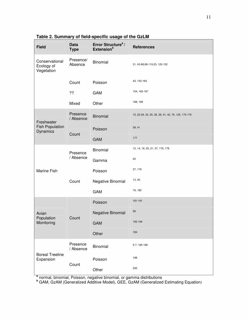
Field specific literature reviews for GzLM usage

Ecology is a broad field that encompasses many sub-disciplines of research, ranging from

the study of microbes to entire ecosystems. In order to investigate the frequency of usage

and specific applications of the GzLM in ecological studies, we therefore felt it was

necessary to do literature reviews which were limited to several specific fields of ecology

(conservational ecology, freshwater and marine fish population dynamics, avian

population monitoring, boreal treeline expansion, and aquatic bacterial abundance). This

method provided results that demonstrate the flexibility provided by the error structure in

the GzLM and its ability to evaluate various types of biological data, along with the

increasing frequency of usage of GzLMs in recent years.

All literature searches were carried out in the databases Web of Science and

Biological Abstracts, using a pre-determined set of statistical query terms, along with

ecological terms specific to each field (Table 1). It was possible that a greater number of

references could have been found using further refined queries, but for the purposes of

comparability across fields we chose to only use the pre-determined set of search terms.

Search results were reviewed to determine if the GzLM was implemented, and if so, what

9

type of data was being analyzed and what error structure was used (binomial, negative

binomial, Poisson, Gamma). Articles in which the error structure was not stated were

recorded as “Other” or on the basis of the extension used (Table 2). The total number of

articles found per year was used to evaluate the frequency of GzLM usage over the past

two decades (Fig. 1).

Of the six fields searched, the only one which did not produce any results was

aquatic bacterial abundance. Within the articles found for conservational ecology,

freshwater and marine fish population dynamics, and boreal treeline expansion, the most

common error structure used was binomial, as presence/absence response variables were

frequently analyzed; within these four fields, there was also some usage of the Poisson

error structure, where response variables were count data (Table 2). The literature search

within avian population trends, however, did not find any articles using binomial error –

the majority of results in this field used Poisson (Table 2), as bird population trends are

typically determined based on count data. Articles were also found which used negative

binomial and Gamma error structures, but these were not as prevalent as binomial and

Poisson (Table 2).

The literature reviews showed that GzLM usage has increased over the past two

decades in all six fields searched (Fig. 1). The general trend produced when all results

were totaled showed that GzLM usage was relatively low in the early 1990’s, but

increased steadily from the mid 1990’s onward (Fig.1,a). Though this literature review

only examined six fields of ecology, this trend appeared to occur across the five which

produced results (Fig.1,b). If further refined searches were conducted and a larger

number of fields surveyed, a more comprehensive picture of GzLM usage in ecology

10

would be obtained. However, the literature review of conservational ecology was fairly

broad and produced a high number of results (131) which included a range of types of

studies (Table 2), possibly indicating the trend for GzLM use in ecology in general.

Table 1. Query terms input into Web of Science and Biological Abstracts for GzLM literature searches

Field specific query terms

Conservational ecology of vegetation Conservation, Ecology, Vegetation

Freshwater fish population dynamics Stream, Fish, Salmonid, Abundance, Distribution, Population

Marine fish population dynamics Demersal/Marine Fish Habitat, Abundance, Distribution

Avian population monitoring Birds, Aves, Population, Trends, Monitoring, Plots, Counts

Treeline expansion Boreal, Treeline, Expansion

Aquatic bacterial abundance Aquatic, Bacteria, Abundance

Statistical query terms

Generalized and Generalised Linear Model(s), Generalized and Generalised Additive Model(s), Generalized and Generalised Estimating Equation, Logistic Regression, Poisson, Binomial, Gamma

11

Table 2. Summary of field-specific usage of the GzLM

Field Data Type

Error Structurea /

Extensionb References

Conservational Ecology of Vegetation

Presence/Absence

Binomial

31, 43-88,89-119,23, 120-152

Count Poisson 43, 153-164

?? GAM 154, 165-167

Mixed Other 168, 169

Presence / Absence

Binomial 15, 22-29, 33, 35, 36, 39, 41, 42, 76, 125, 170-176

Poisson 39, 41

Freshwater Fish Population Dynamics

Count

GAM 177

Binomial 12, 14, 18, 20, 21, 37, 176, 178

Presence / Absence

Gamma 20

Poisson 37, 179

Negative Binomial 13, 40

Marine Fish

Count

GAM 19, 180

Poisson 181-191

Negative Binomial 58

GAM 192-194

Avian Population Monitoring

Count

Other 184

Presence / Absence

Binomial 5-7, 195-199

Poisson 198

Boreal Treeline Expansion

Count

Other 200

a normal, binomial, Poisson, negative binomial, or gamma distributions

b GAM, GzAM (Generalized Additive Model), GEE, GzAM (Generalized Estimating Equation)

12

Figure 1. Frequency of GzLM usage resulting from literature searches of five ecological fields. (a) Frequency of usage in each field (b) Total incidence of usage, pooled from all searches.

(b)

(a)

13

Statistical analysis and summary of ecological data sets

GLMs and GzLMs were computed in the statistical programs SAS (9.1), R (2.6) and

Minitab (13).

As seen in Table 3, one data set (B) could not be analyzed using the GLM,

therefore this analysis is not included in the comparison of model results. From the

remaining data sets, 13 of 21 parameters were significant when the GzLM was applied.

Of these 13 parameters, 8 showed a decrease in p value from the GLM – 2 of which had

not been significant until the application of the GzLM. The remaining 6 significant

parameters had p values less than 0.001 and were not evaluated for change. Of the 8 non-

significant parameters, 5 showed a decrease upon the application of the GzLM.

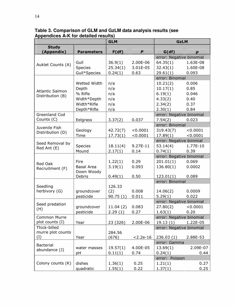
14

Table 3. Comparison of GLM and GzLM data analysis results (see Appendices A-K for detailed results)

GLM GzLM

Study

(Appendix) Parameters F(df) P G(df) p

error: Negative binomial

Gull 36.9(1) 2.00E-06 64.35(1) 1.63E-08

Species 25.34(1) 3.01E-05 32.43(1) 1.60E-08 Auklet Counts (A)

Gull*Species 0.24(1) 0.63 29.61(1) 0.093

error: Binomial

Wetted Width n/a 10.21(2) 0.006

Depth n/a 10.17(1) 0.85

% Rifle n/a 6.19(1) 0.046

Width*Depth n/a 4.33(2) 0.40

Width*Rifle n/a 2.34(2) 0.37

Atlantic Salmon

Distribution (B)

Depth*Rifle n/a 2.30(1) 0.84

error: Negative binomial Greenland Cod

Counts (C) Eelgrass 3.37(2) 0.037 7.54(2) 0.023

error: Binomial

Geology 42.72(7) <0.0001 319.43(7) <0.0001 Juvenile Fish

Distribution (D) Time 17.73(1) <0.0001 17.89(1) <0.0001

error: Negative binimial

Species 18.11(4) 9.27E-11 53.14(4) 1.77E-10 Seed Removal by

Red Ant (E) Mound 2.17(1) 0.14 0.74(1) 0.39

error: Begative binomial

Fire 1.22(1) 0.29 201.01(1) 0.069

Basal Area 3.19(1) 0.093 136.80(1) 0.0002 Red Oak

Recruitment (F) Down Woody

Debris 0.49(1) 0.50 123.01(1) 0.089

error: Binomial

groundcover

126.33

(2) 0.008 14.06(2) 0.0009

Seedling

herbivory (G)

pesticide 90.75 (1) 0.011 5.29(1) 0.022

error: Negative binomial

groundcover 11.04 (2) 0.083 27.80(2) <0.0001 Seed predation

(H) pesticide 2.29 (1) 0.27 1.63(1) 0.20

error: Negative binomial Common Murre

plot counts (I) Year 23 (326) 2.00E-06 19.13 (1) 1.22E-05

error: Negative binomial Thick-billed

murre plot counts

(I) Year

284.56

(676) <2.2e-16 236.03 (1) 2.88E-53

error: Gamma

water masses 19.57(1) 4.00E-05 13.69(1) 2.09E-07 Bacterial

abundance (J) pH 0.11(1) 0.74 0.24(1) 0.44

error: Poisson

dishes 1.36(1) 0.25 1.21(1) 0.27 Colony counts (K)

quadratic 1.55(1) 0.22 1.37(1) 0.25

15

Advantages and disadvantages to applying the GzLM

Over the duration of the Biology 7932 graduate course, we developed our understanding

of the generalized linear model and how to apply it to data with a non-normal error

distribution. From our analyses, we have discovered some general problems that arise

when using the GzLM, some of them particular to our exemplary data sets. Here, we

discuss advantages and disadvantages inherent to applying the GzLM to data with

Poisson, negative binomial, binomial and gamma distributions. Some were problems

directly encountered during the analysis of the exemplary data sets, and some are more

general limitations drawn from various ecological studies.

Poisson and negative binomial distributions

The generalized linear model can be applied to data with both the Poisson and negative

binomial distribution. The Poisson distribution is usually linked to count data, which

commonly appears in ecological literature; count data are generated through studies that

gather model information through mark-recapture experiments170, site-specific captures

such as trawls13 and plot counts, a common method of evaluating seabird populations172,

181.

Population monitoring of birds almost always relies on surveys of a sample

population 201. This is because it is not feasible to census the entire population of most

birds. Consequently, censuses of large colonies are usually based on sub-samples of the

population202. In this section we review the analysis of long-term count data from census

plots at Cape St. Mary’s, Newfoundland, 1980-2006 (Appendix I).

16

The analysis of count data is often complicated due to the subjective nature of

trend estimation and high inherent variation. There are many statistical techniques that

may be employed to analyze count data, however, there is little consensus regarding the

most suitable method 201. Linear regression is one of the oldest statistical technique, and

has been long been used in ecological research to test trends. When a linear regression

model was fit to the Cape St. Mary’s common murre plot data, we found that it

preformed poorly, exhibiting non-normal, non-independent and heterogeneous residuals.

A second option is to run a GzLM with a Poisson distribution (Poisson

regression). Poisson regression is a frequently used method for count data. A key feature

of Poisson distribution is that it assumes that as the mean increases, the variance

increases – which is a frequent characteristic of count data4. Nevertheless, it appears that

the murre count observations exceeded the amount of variation predicted by Poisson,

whereby the estimated overdispersion parameter (φ [Null deviance/df]) was much greater

than 1 (φ = 8.9). The Poisson distribution may have fit the data poorly since it is

designed to be used for counts of events that occur randomly over time or space203. The

murre plot count data are neither temporally or spatially independent since counts are

conducted at the same time for all plots and the same plots are monitored across years.

The negative binomial is a distribution related to Poisson, however it includes an

extra parameter (dispersion parameter) which allows the variance to exceed the mean204.

Counts of populations are often fitted well by the negative binomial distribution205.

White and Bennetts206 suggest that ecological count data likely exhibit a negative

binomial distribution more frequently than Poisson or normal distributions. When a

17

GzLM with a negative binomial distribution was fitted to the murre plot data, the

overdispersion parameter was much closer to 1 (φ = 1.1).

As apparent from the analysis of the Cape St. Mary’s murre plot trend data, one of

the main advantages of GzLMs over GLMs is that they do not force data into unnatural

scales by allowing for non-consistent variance structures in the data. Linear regression

models are limited by the assumptions that the errors are identical, independently, and

normally distributed. In the case of the murre count data, the GzLM model allowed for

the selection of different distributions such as Poisson or negative binomial, which better

suited the data. Within the options available in the GzLM, the negative binomial

distribution appeared to best suit the data. The dispersion parameter accounted for the

extra variance which exceeded the assumptions in the Poisson regression.

The main disadvantage of the Poisson distribution is that the scope of data that

can be analyzed using this distribution is limited by the assumption that the mean

increases with the variance. The Poisson distribution do not account for any extra

variation in the data, thus in such cases, a negative binomial distribution may be more

appropriate. The primary disadvantage of using negative binomial regression is that there

are fewer programs that are capable of building a GzLM with a negative binomial

distribution. Another disadvantage of the negative binomial distribution is the inclusion

of the dispersion parameter. With an increase in parameters, there is a decrease in

precision and one may run the risk of overfitting the data, thus less weight should be

placed on models with a higher number of parameters136. One general disadvantage of

the GzLM is the lack of diagnostic plots available to assess the model. One specific

problem relating to the count data is in the estimation and assessment of the

18

overdispersion parameter – there appears to be no standard method of calculation, or a

definition of how much the estimate needs to deviate from 1 for the data to be considered

overdispersed.

Binomial distributions

Binomial data is common in ecological modelling. It often appears as presence / absence

or risk data, which is binary in nature, so unlike other non-normal distributions, it is

usually relatively easy to determine when to apply the GzLM with a binomial

distribution. When the data are binary and the distribution is accepted as non-Gaussian,

the data are usually analysed using logistic regression. Logistic regression is a GzLM

analysis that is often used in ecological research; it has been applied for evaluating

habitat207, assessing risk208, and predicting the distribution of species and vegetation

groups6, 209.

The seedling herbivory data collected in the Mealy Mountains during the summer

of 2007 (See Appendix G for details) demonstrate a clear example of a binomial response

variable (in this case, herbivory occurs or does not occur for each seedling). The purpose

of the study was to determine whether the odds of herbivory were influenced by a variety

of environmental factors; since the response variable is binary, we assumed a binomial

distribution and applied a logistic regression model.

A limitation of the GzLM was encountered when analysing the binomial seedling

herbivory data; here, we review the difficulty in performing a prospective power analysis

for a logistic regression model. A prospective power analysis is used to help the

researcher design their study, ensuring that the effect size, sample size, and level of

19

precision are all sufficiently large to generate an experiment with sufficient statistical

power210. A prospective power analysis was performed using the SAS macro UnifyPow

on the herbivory logistic regression model in order to determine the increase in sample

size needed to maintain the power of the study through a second experimental season;

since seedlings were being removed through herbivory, the sample size (and thus the

power) was decreasing over time. However, according to the power analysis, the power

of the study remained equal regardless of any increases in the initial population size. The

problems of prospective power analyses and their application to binomial GzLMs are not

well documented in the ecological literature. Power analyses for logistic regression

models are generally used in medical studies211 , but these cannot be easily compared to

ecological studies.

In general, there are some limitations to the application of the GzLM for

analysing binary data generated by ecological studies. In ecology and conservation

biology, logistic regression models are relatively common, and often used for modelling

spatial species distributions under different environmental conditions6, 199. However,

these models must assume that the species is in a state of pseudo-equilibrium with the

environment; therefore, logistic regression models cannot effectively identify

environmental factors responsible for distribution when a species is not in equilibrium, or

still expanding its range3. Furthermore, GzLMs and GAMs are usually based on

empirical data collected from a particular region, thus incorporating the biotic

interactions and random effects that are characteristic to the area. This means that

predictive GzLMs designed for one region usually cannot be applied on a wider scale; the

predictive power over a broad spatial scale is usually low3, 212. Another general

20

disadvantage of logistic regression analysis is the tendency of the model to strongly

underestimate the probability of rare events213.

Gamma distributions

The gamma distribution also occurs in ecological studies, though much less frequently

than binomial and Poisson according to our literature search. Thus, there is less

information available about its application to ecological data. The gamma distribution is

a 2-parameter frequency distribution given by the equation:

0,0;)(

1)( /1 >>

Γ= −− γβ

γββγ

γ

xexxf

Gamma distribution has a zero lower bound and is unlimited on the right. It is positively

skewed, with the amount of skew depending inversely on the shape factor γ . The

gamma distribution is closely related to the Chi-square distribution, for 2/2χ is a gamma

variate214.

In biological ecology, data distributions are highly variable; as we have observed,

most data are not normally distributed. The general linear model is usually applied when

the distribution is gamma; this occurs partially because basic linear statistics (based on

the normal distribution) have been traditionally and widely taught. The major advantage

of using the gamma distribution is that it simplifies the interpretation of the model; if you

force the model to fit the normal distribution where gamma is applicable, the variables

need to be transformed, which complicates the biological interpretation of the parameters.

Gamma distribution helps expand the capacity of data analysis without using

transformation. The major disadvantage of using the gamma distribution is common to

many applications of the generalized linear model; in order to analyse a model using

21

gamma distribution, you need a powerful statistical software package and also relatively

advanced knowledge of statistics.

Conclusions

The GzLM has become increasingly common in ecological studies over the past two

decades. This is largely due to the flexibility of the GzLM when compared to the GLM,

in that it does not assume normal distributions. The nature of ecological data often

produces data which is highly varied, has counts with many zeros, is over dispersed,

skewed, or more suited to analysis of presence versus absence. The specification of the

error structure in the GzLM allows ecological researchers to create models which can

account for the nature of these datasets and provide more meaningful statistical analysis.

Despite these advantages of GzLMs, their use has not become widespread until recently.

It is likely that as the acceptance and discussion of the GzLM increases, its role as the

most appropriate model for ecological data analysis will be recognized in the field.

Acknowledgements

The authors of this paper wish to thank Dr. David Schneider for offering the Biology

7932 graduate course, Applications of the Generalized Linear Model, and for his

assistance and support during data analysis and the writing of this paper. Thanks also to

Dr. Keith Lewis and Peter Westley for their assistance during data analysis. Additional

thanks to Dr. Paul Marino and Dr. Dave Cote for providing extra data sets.

22

References

1. Shenk, T.M., and Franklin, A.B. (2001) Modeling in Natural Resource

Management: Development, Interpretation, and Application. Island Press 2. Nelder, J.A., and Wedderburn, R.W.M. (1972) Generalized Linear Models. J. R.

Stat. Soc. A. 135, 370-384 3. Guisan, A., et al. (2002) Generalized linear and generalized additive models in studies of species distributions: setting the scene. Ecol. Model. 157, 89-100 4. Agresti, A. (2007) An Introduction to categorical data analysis. Wiley-Interscience 5. Bolliger, J.F., and al., e. (2000) Risks of global warming on montane and subalpine forests in Switzerland – a modeling study. Remote Sensing of Environment 1, 99-111 6. Calef, M.P., et al. (2005) Analysis of vegetation distribution in interior Alaska and sensitivity to climate change using a logistic regression approach. J. Biogeography 32, 863-878 7. Leniham, J.M. (1993) Ecological response surfaces for North American boreal tree species and their use in forest classification. J. Veg. Sci. 4, 667-680 8. He, F., et al. (2003) Autologistic regression model for the distribution of vegetation. Journal of Agricultural, Biological, and Environmental Statistics 8, 205-222 9. Kirchman, D.L. (2000) Microbial Ecology of the Oceans. Wiley 10. Karner, M.B., et al. (2001) Archeal dominance in the mesopelagic zone of the Pacific Ocean. Nature 409 11. Sousa1, P., et al. (2007) Analysis of horse mackerel, blue whiting, and hake catch data from Portuguese surveys (1989-1999) using an integrated GLM approach. . Aquat.

Living Resour. 20, 105-116 12. Maravelias, C.D. (1999) Habitat selection and clustering of pelagic fish: effects of topography and bathymetry on species dynamics. Can. J. Fish. Aquat. Sci. 56, 437–450 13. Jarvela, L.E., and Thorsteinson, L.K. (1999) The epipelagic fish community of Beaufort Sea coastal waters, Alaska Arctic 52, 80-94 14. Byrkjedal, I., and Hoines, A. (2007) Distribution of demersal fish in the south-western Barents Sea. Polar Research 26, 135–151 15. Dauwalter, D.C., and Fisher, W.L. (2007) Electrofishing capture probability of smallmouth bass in streams. N.A. J. Fish. Man 27, 162-171 16. Lusk, S., and Humpl (2006) Effect of multiple electrofishing on determining the structure of fish communities in small streams. Folia. Zool. 55, 315-322. 17. Venables, W.N., and Dichmont, C.M. (2004) GLMs, GAMs and GLMMs: An overview of theory for applications in fisheries research. Fish. Res. 70, 319-337 18. Crawley, K.R., et al. (2006) Influence of different volumes and types of detached macrophytes on fish community structure in surf zones of sandy beaches. Mar. Ecol.

Prog. Ser 307, 233-246

23

19. Stoner, A., et al. (2003) Spatially explicit analysis of estuarine habitat for juvenile winter flounder: Combining generalized additive models and geographic information systems. Mar. Ecol. Prog. Ser. 213, 252-271 20. Sousa, P., et al. (2007) Analysis of horse mackerel, blue whiting, and hake catch data from Portuguese surveys (1989-1999) using an integrated GLM approach. . Aquat.

Living Resour. 20, 105-116 21. Schick, R.S., et al. (2004) Bluefin tuna (Thunnus thynnus) distribution in relation to sea surface temperature fronts in the Gulf of Maine (1994-96). Fish. Ocean. 13, 225-238 22. Dunham, J.B., and Rieman, B.E. (1999) Metapopulation structure of bull trout: Influences of physical, biotic and geometrical landscape characteristics. Ecol. App. 9, 642-667 23. Eikaas, H.S., et al. (2005) Spatial modeling and habitat quantification for two diadromous fish in New Zealand streams: GIS-based approach with application for conservation management. Environmental-Management 36, 726-740 24. Flebbe, P.A. (1994) A regional view of the margin: Salmonid abundance and distribution in the southern Appalachian mountains of North Carolina and Virginia. Trans. Amer. Fish. Soc. 123, 657-667 25. Garland, R.D., et al. (2002) Comparison of subyearling fall Chinook salmon's use of riprap revetments and unaltered habitats in Lake Wallula of the Columbia River. N.A.

J. Fish. Man. 22, 1283–1289 26. Latterell, J.J., et al. (2003) Physical constraints on trout (Oncorhynchus spp.) distribution in the Cascade Mountains: a comparison of logged and unlogged streams. 27. Porter, M.S., et al. (2000) Predictive models of fish species distribution in the Blackwater Drainage, British Columbia. N.A. J. Fish. Man. 20, 349–359 28. Press, G.R., et al. (2002) Landscape characteristics, land use, and coho salmon (Oncorhynchus kisutch) abundance, Snohomish River, Wash., U.S.A. Can. J. Fish.

Aquat. Sci. 59, 613-623 29. Rieman, B.E., and McIntyre, J.D. (1995) Occurrence of bull trout in naturally fragmented habitat patches of varied size. Trans. Amer. Fish. Soc. 124, 285–296 30. Tiffan, K.F., et al. (2006) Variables influencing the presence of subyearling fall Chinook salmon in shoreline habitats of the Hanford Reach, Columbia River. N.A. J.

Fish. Man. 26, 351-360 31. Watson, G., and Hillman, T.W. (1997) Factors affecting the distribution and abundance of bull trout: An investigation at hierarchical scales. North-American-Journal-

of-Fisheries-Management 17, 237-252 32. Welsh, H.H., et al. (2001) Distribution of juvenile Coho salmon in relation to water temperatures in tributaries of the Mattole River, California. . N.A. J. Fish. Man. 21, 464-470. 33. Mugodo, J. (2006) Evalution and application of methods for biological assessment of streams. Hydrobiologia 572, 59-70 34. Girard, I.L., et al. (2004) Foraging, growth, and loss rate of young-of-the-year Atlantic salmon (Salmo salar) in relation to habitat use in Catamaran Brook, New Brunswick. Can. J. Fish. Aquat. Sci. 61, 2339-2349

24

35. Kocovsky, P.M., and Carline, R.F. (2006) Influence of landscape-scale factors in limiting brook trout populations in Pennsylvania streams. Trans. Amer. Fish. Soc. 135, 76-88 36. Knapp, R.A., and Preisler, H.K. (1999) Is it possible to predict habitat use by spawning salmonids? A test using California golden trout (Oncorhynchus mykiss

aguabonita). Can. J. Fish. Aquat. Sci. 56, 1576-1584 37. Francis, M.P., and al., e. (2005) Predictive models of small fish presence and abundance in northern New Zealand harbours. Estuarine, Costal and Shelf Science 62 38. Santoul, F., et al. (2005) Environmental factors influencing the regional distribution and local density of a small benthic fish: The stoneloach (Barbatula

barbatula). Hydrobiologia 544 347-355 39. Santoul, F., et al. (2005) Patterns of rare fish and aquatic insects in a southwestern French river catchment in relation to simple physical variables. Ecography 28, 307-314 40. Greenwood, M.F.D., and Hill, A.S. (2003) Temporal, spatial and tidal influences on benthic and demersal fish abundance in the Fourth estuary. Eustarine, Costal and

Shelf Sci. 28, 211-225 41. Rosenfeld, J., et al. (2000) Habitat factors affecting the abundance and distribution of juvenile cutthroat trout (Oncorhynchus clarki) and Coho salmon (Oncorhynchus kisutch). Can. J. Fish. Aquat. Sci. 57, 766-774 42. Ripley, T.e.a., et al. (2005) Bull trout (Salvelinus confluentus) occurrence and abundance influenced by cumulative industrial developments in Canadian boreal forest watershed. Can. J. Fish. Aquat. Sci. 62, 2431-2442 43. Olivera-Gomez, L.D., and Mellink, E. (2005) Distribution of the Antillean manatee (Trichechus manatus manatus) as a function of habitat characteristics, in Bahia de Chetumal, Mexico. Biological-Conservation 121, 127-133 44. Williams, N.S.G., et al. (2005) Plant traits and local extinctions in natural grasslands along an urban-rural gradient. Journal of Ecology 93, 1203-1213 45. Polak, M. (2007) Nest-site selection and nest predation in the Great Bittern Botaurus stellaris population in eastern Poland. Ardea 95, 31-38 46. Millington, J.D.A., et al. (2007) Regression techniques for examining land use/cover change: A case study of a mediterranean landscape. Ecosystems 10, 562-578 47. Hein, S., et al. (2007) Habitat suitability models for the conservation of thermophilic grasshoppers and bush crickets - simple or complex? Journal of Insect

Conservation 11, 221-240 48. Gibson, L.A., et al. (2004) Modelling habitat suitability of the swamp antechinus (Antechinus minimus maritimus) in the coastal heathlands of southern Victoria, Australia. Biological Conservation 117, 143-150 49. Garcia-Ripolles, C., et al. (2005) Modelling nesting habitat preferences of Eurasian Griffon Vulture Gyps fulvus in eastern Iberian Peninsula. Ardeola 52, 287-304 50. Zabala, J., et al. (2006) Facteurs affectant l'habitat du vison en Europe sud-occidentale. Mammalia- 70, 193-201 51. Yap, C.A.M., et al. (2002) Roost characteristics of invasive mynas in Singapore. Journal-of-Wildlife-Management 66, 1118-1127 52. Wood, D.R., et al. (2004) Avian community response to pine-grassland restoration. Wildlife-Society-Bulletin 32, 819-828

25

53. Wiser, S.K., et al. (1998) Prediction of rare-plant occurrence: A southern appalachian example. Ecological-Applications 8, 909-920 54. Wilson, S.M., et al. (2006) Landscape conditions predisposing grizzly bears to conflicts on private agricultural lands in the western USA. Biological-Conservation 130, 47-59 55. Wilson, B.A., and Aberton, J.G. (2006) Effects of landscape, habitat and fire on the distribution of the white-footed dunnart Sminthopsis leucopus (Marsupialia : Dasyuridae) in the Eastern Otways, Victoria. Australian-Mammalogy 28, 27-38 56. Williams, N.S.G., et al. (2005) Factors influencing the loss of an endangered ecosystem in an urbanising landscape: a case study of native grasslands from Melbourne, Australia. Landscape-and-Urban-Planning 71, 35-49 57. Williams, N.S.G. (2007) Environmental, landscape and social predictors of native grassland loss in western Victoria, Australia. Biological-Conservation 137, 308-318 58. White, P.C.L., et al. (2003) Factors affecting the success of an otter (Lutra lutra) reinforcement programme, as identified by post-translocation monitoring. Biological-

Conservation 112, 363-371 59. Westphal, M.I., et al. (2003) Effects of landscape pattern on bird species distribution in the Mt. Lofty Ranges, South Australia. Landscape-Ecology 18, 413-426 60. Welch, N.E., and MacMahon, J.A. (2005) Identifying habitat variables important to the rare Columbia spotted frog in utah (USA): An information-theoretic approach. Conservation-Biology 19, 473-481 61. Ward, L., and Mill, P.-J. (2005) Habitat factors influencing the presence of adult Calopteryx splendens (Odonata : Zygoptera). European-Journal-of-Entomology 102, 47-51 62. Vanreusel, W., and Van-Dyck, H. (2007) When functional habitat does not match vegetation types: A resource-based approach to map butterfly habitat. Biological-

Conservation 135, 202-211 63. vandenBerg, L.J.L., et al. (2001) Territory selection by the Dartford warbler (Sylvia undata) in Dorset, England: The role of vegetation type, habitat fragmentation and population size. Biological-Conservation 101, 217-228 64. Toner, M., and Keddy, P. (1997) River hydrology and riparian wetlands: A predictive model for ecological assembly. Ecological-Applications 7, 236-246 65. Tittler, R., and Hannon, S.J. (2000) Nest predation in and adjacent to cutblocks with variable tree retention. Forest-Ecology-and-Management 136, 147-157 66. Thomson, J.R., et al. (2007) Predicting bird species distributions in reconstructed landscapes. Conservation-Biology 21, 752-766 67. Suarez, F., et al. (2003) The role of extensive cereal crops, dry pasture and shrub-steppe in determining skylark Alauda arvensis densities in the Iberian peninsula. Agriculture-Ecosystems-and-Environment 95, 551-557 68. Stoleson, S.H., and Finch, D.M. (2003) Microhabitat use by breeding Southwestern Willow Flycatchers on the Gila River, New Mexico. Studies-in-Avian-

Biology, 91-95 69. Soh, M.C.K., et al. (2006) High sensitivity of montane bird communities to habitat disturbance in Peninsular Malaysia. Biological-Conservation 129, 149-166 70. Singer, F.J., et al. (2000) Correlates to colonizations of new patches by translocated populations of bighorn sheep. Restoration-Ecology 8, 66-74

26

71. Robbins, C.S., et al. (1989) Habitat Area Requirements of Breeding Forest Birds of the Middle Atlantic States USA. Wildlife-Monographs, 1-34 72. Rivieccio, M., et al. (2003) Habitat features and predictive habitat modeling for the Colorado chipmunk in southern New Mexico. Western-North-American-Naturalist 63, 479-488 73. Ritter, M.W., and Savidge, J.A. (1999) A predictive model of wetland habitat use on Guam by endangered Mariana Common Moorhens. Condor- 101, 282-287 74. Reich, R.M., et al. (2004) Predicting the location of northern goshawk nests: modeling the spatial dependency between nest locations and forest structure. Ecological-

Modelling 176, 109-133 75. Radford, J.Q., and Bennett, A.F. (2004) Thresholds in landscape parameters: occurrence of the white-browed treecreeper Climacteris affinis in Victoria, Australia. Biological-Conservation 117, 375-391 76. Quist, M.C., et al. (2005) Hierarchical faunal filters: an approach to assessing effects of habitat and nonnative species on native fishes. Ecology-of-Freshwater-Fish 14, 24-39 77. Quintana-Ascencio, P.F., and Menges, E.S. (1996) Inferring metapopulation dynamics from patch-level incidence of Florida scrub plants. Conservation-Biology 10, 1210-1219 78. Puglisi, L., et al. (2005) Man-induced habitat changes and sensitive species: a GIS approach to the Eurasian Bittern (Botaurus stellaris) distribution in a Mediterranean wetland. Biodiversity-and-Conservation 14, 1909-1922 79. Pueyo, Y., et al. (2006) Determinants of land degradation and fragmentation in semiarid vegetation at landscape scale. Biodiversity-and-Conservation 15, 939-956 80. Plentovich, S., et al. (1999) Habitat requirements for Henslow's sparrows wintering in silvicultural lands of the Gulf Coastal Plain. Auk- 116, 109-115 81. Pleasant, G.D., et al. (2006) Nesting ecology and survival of scaled quail in the Southern High Plains of Texas. Journal-of-Wildlife-Management 70, 632-640 82. Pausas, J.G. (1997) Resprouting of Quercus suber in NE Spain after fire. Journal-

of-Vegetation-Science 8, 703-706 83. Partl, E., et al. (2002) Forest restoration and browsing impact by roe deer. Forest-

Ecology-and-Management 159, 87-100 84. Parker, J.M., and Anderson, S.H. (2003) Habitat use and movements of repatriated Wyoming toads. Journal-of-Wildlife-Management 67, 439-446 85. Oostermeijer, J.G.B., and Van-Swaay, C.A.M. (1998) The relationship between butterflies and environmental indicator values: A tool for conservation in a changing landscape. Biological-Conservation 86, 271-280 86. Nielsen, S.E., et al. (2004) Modelling the spatial distribution of human-caused grizzly bear mortalities in the Central Rockies ecosystem of Canada. Biological-

Conservation 120, 101-113 87. Ng, S., and Corlett, R.T. (2003) The ecology of six Rhododendron species (Ericaceae) with contrasting local abundance and distribution patterns in Hong Kong, China. Plant-Ecology 164, 225-233 88. Nepal, S.K. (2003) Trail impacts in Sagarmatha (Mt. Everest) National Park, Nepal: A logistic regression analysis. Environmental-Management 32, 312-321

27

89. Naura, M., and Robinson, M. (1998) Principles of using River Habitat Survey to predict the distribution of aquatic species: An example applied to the native white-clawed crayfish Austropotamobius pallipes. Aquatic-Conservation 8, 515-527 90. Munger, J.C., et al. (1998) U.S. national wetland inventory classifications as predictors of the occurrence of Columbia spotted frogs (Rana luteiventris) and Pacific treefrogs (Hyla regilla). Conservation-Biology 12, 320-330 91. Mortberg, U.M., and Wallentinus, H.G. (2000) Red-listed forest bird species in an urban environment: Assessment of green space corridors. Landscape-and-Urban-

Planning 50, 215-226 92. Mortberg, U.M. (2001) Resident bird species in urban forest remnants; landscape and habitat perspectives. Landscape-Ecology 16, 193-203 93. Moran-Lepez, R., et al. (2005) Summer habitat relationships of barbels in south-west Spain. Journal-of-Fish-Biology 67, 66-82 94. Miller, J.R., and Cale, P. (2000) Behavioral mechanisms and habitat use by birds in a fragmented agricultural landscape. Ecological-Applications 10, 1732-1748 95. Meyer, C.B., and Miller, S.L. (2002) Use of fragmented landscapes by marbled murrelets for nesting in southern Oregon. Conservation-Biology 16, 755-766 96. McKee, G., et al. (1998) Predicting greater prairie-chicken test success from vegetation and landscape characteristics. Journal-of-Wildlife-Management 62, 314-321 97. McComb, W.C., et al. (2002) Models for mapping potential habitat at landscape scales: An example using northern spotted owls. Forest-Science 48, 203-216 98. Mazzocchi, A.B., and Forys, E.A. (2005) Nesting habitat selection of the Least Tern on the Gulf Coast of Florida. Florida-Field-Naturalist 33, 71-80 99. Marsden, S., and Fielding, A. (1999) Habitat associations of parrots on the Wallacean islands of Buru, Seram and Sumba. Journal-of-Biogeography 26, 439-446 100. Manel, S., et al. (2000) Testing large-scale hypotheses using surveys: The effects of land used on the habitats, invertebrates and birds of Himalayan rivers. Journal-of-

Applied-Ecology 37, 756-770 101. Mallord, J.W., et al. (2007) Linking recreational disturbance to population size in a ground-nesting passerine. Journal-of-Applied-Ecology 44, 185-195 102. Madden, E.M., et al. (2000) Models for guiding management of prairie bird habitat in northwestern North Dakota. American-Midland-Naturalist 144, 377-392 103. MacFaden, S.W., and Capen, D.E. (2002) Avian habitat relationships at multiple scales in a New England forest. Forest-Science 48, 243-253 104. Lindenmayer, D.B., and McCarthy, M.A. (2001) The spatial distribution of non-native plant invaders in a pine-eucalypt landscape mosaic in south-eastern Australia. Biological-Conservation 102, 77-87 105. Li, X., et al. (2006) Nest site use by crested ibis: dependence of a multifactor model on spatial scale. Landscape-Ecology 21, 1207-1216 106. Lehtinen, R.M., and Skinner, A.A. (2006) The enigmatic decline of Blanchard's Cricket Frog (Acris crepitans blanchardi): A test of the habitat acidification hypothesis. Copeia-, 159-167 107. Lantin, E., et al. (2003) Preliminary assessment of habitat characteristics of woodland caribou calving areas in the Claybelt region of Quebec and Ontario, Canada. Rangifer-, 247-254

28

108. Jones, J.C., and Dorr, B. (2004) Habitat associations of gopber tortoise burrows on industrial timberlands. Wildlife-Society-Bulletin 32, 456-464 109. Johnson, B.K., et al. (2000) Resource selection and spatial separation of mule deer and elk during spring. Journal-of-Wildlife-Management 64, 685-697 110. Jimenez, I. (2005) Development of predictive models to explain the distribution of the West Indian manatee Trichechus manatus in tropical watercourses. Biological-

Conservation 125, 491-503 111. Jeganathan, P., et al. (2004) Modelling habitat selection and distribution of the critically endangered Jerdon's courser Rhinoptilus bitorquatus in scrub jungle: an application of a new tracking method. Journal-of-Applied-Ecology 41, 224-237 112. Hornung, J.P., and Rice, C.L. (2003) Odonata and wetland quality in southern Alberta, Canada: A preliminary study. Odonatologica- 32, 119-129 113. Hodar, J.A., et al. (2000) Habitat selection of the common chameleon (Chamaeleo chamaeleon) (L.) in an area under development in southern Spain: Implications for conservation. Biological-Conservation 94, 63-68 114. Hill, J.K. (1999) Butterfly spatial distribution and habitat requirements in a tropical forest: Impacts of selective logging. Journal-of-Applied-Ecology 36, 564-572 115. Hazler, K.R., et al. (2006) Factors influencing acadian flycatcher nesting success in an intensively managed forest landscape. Journal-of-Wildlife-Management 70, 532-538 116. Hatten, J.R., and Paradzick, C.E. (2003) A multiscaled model of southwestern willow flycatcher breeding habitat. Journal-of-Wildlife-Management 67, 774-788 117. Hancock, M.H., and Wilson, J.D. (2003) Winter habitat associations of seed-eating passerines on Scottish farmland. Bird-Study 50, 116-130 118. Guenette, J.S., and Villard, M.A. (2005) Thresholds in forest bird response to habitat alteration as quantitative targets for conservation. Conservation-Biology 19, 1168-1180 119. Gros, P.M., and Rejmanek, M. (1999) Status and habitat preferences of Uganda cheetahs: An attempt to predict carnivore occurrence based on vegetation structure. Biodiversity-and-Conservation 8, 1561-1583 120. Groenendijk, J.P., et al. (2005) Successional position of dry Andean dwarf forest species as a basis for restoration trials. Plant-Ecology 181, 243-253 121. Green, R.E., and Stowe, T.J. (1993) The decline of the corncrake Crex crex in Britain and Ireland in relation to habitat change. Journal-of-Applied-Ecology 30, 689-695 122. Giroux, W., et al. (2007) Ruffed grouse brood habitat use in mixed softwood-hardwood nordic-temperate forests, Quebec, Canada. Journal-of-Wildlife-Management 71, 87-95 123. Gibson, L.A., et al. (2004) Spatial prediction of rufous bristlebird habitat in a coastal heathland: a GIS-based approach. Journal-of-Applied-Ecology 41, 213-223 124. Franco, A.M.A., et al. (2000) Modelling habitat selection of Common Cranes Grus grus wintering in Portugal using multiple logistic regression. Ibis- 142, 351-358 125. Filipe, A.F., et al. (2002) Spatial modelling of freshwater fish in semi-arid river systems: A tool for conservation. River-Research-and-Applications 18, 123-136 126. Field, S.A., et al. (2005) Improving the efficiency of wildlife monitoring by estimating detectability: a case study of foxes (Vulpes vulpes) on the Eyre Peninsula, South Australia. Wildlife-Research 32, 253-258

29

127. Fattebert, K., et al. (2003) Model development for capercaillie (Tetrao urogallus) habitat in the Jura mountains (Western Switzerland). Game-and-Wildlife-Science 20, 195-210 128. Etter, A., et al. (2006) Modelling the conversion of Colombian lowland ecosystems since 1940: Drivers, patterns and rates. Journal-of-Environmental-

Management 79, 74-87 129. Dirnbock, T., et al. (2003) Predicting future threats to the native vegetation of Robinson Crusoe island, Juan Fernandez Archipelago, Chile. Conservation-Biology 17, 1650-1659 130. Daws, M.I., et al. (2006) Prediction of desiccation sensitivity in seeds of woody species: A probabilistic model based on two seed traits and 104 species. Annals-of-

Botany-(London) 97, 667-674 131. Curtis, P.D., and Jensen, P.G. (2004) Habitat features affecting beaver occupancy along roadsides in New York state. Journal-of-Wildlife-Management 68, 278-287 132. Cunningham, S.C., et al. (2003) Black bear habitat use in burned and unburned areas, central Arizona. Wildlife-Society-Bulletin 31, 786-792 133. Chalmers, R.J., and Loftin, C.S. (2006) Wetland and microhabitat use by nesting Four-Toed Salamanders in Maine. Journal-of-Herpetology 40, 478-485 134. Carroll, C., et al. (1999) Using presence-absence data to build and test spatial habitat models for the fisher in the Klamath region, U.S.A. Conservation-Biology 13, 1344-1359 135. Burger, L.D., et al. (1994) Effects of prairie fragmentation on predation on artificial nests. Journal-of-Wildlife-Management 58, 249-254 136. Buchanan, J.B., et al. (1999) Characteristics of young forests used by spotted owls on the western Olympic Peninsula, Washington. Northwest-Science 73, 255-263 137. Bombay, H.L., et al. (2003) Scale perspectives in habitat selection and animal performance for Willow Flycatchers (Empidonax traillii) in the central Sierra Nevada, California. Studies-in-Avian-Biology, 60-72 138. Bisson, I.A., and Stutchbury, B.J.M. (2000) Nesting success and nest-site selection by a neotropical migrant in a fragmented landscape. Canadian-Journal-of-

Zoology 78, 858-863 139. Bigler, C., et al. (2005) Multiple disturbance interactions and drought influence fire severity in rocky mountain subalpine forests. Ecology-(Washington-D-C) 86, 3018-3029 140. Benoit, L.K., and Askins, R.A. (2002) Relationship between habitat area and the distribution of tidal marsh birds. Wilson-Bulletin 114, 314-323 141. Beauvais, G.P., and Smith, R. (2003) Model of breeding habitat of the Mountain Plover (Charadrius montanus) in western Wyoming. Western-North-American-Naturalist 63, 88-96 142. Baumann, M., et al. (2005) Native or naturalized? Validating alpine chamois habitat models with archaeozoological data. Ecological-Applications 15, 1096-1110 143. Baldi, A., and Kisbenedek, T. (1998) Factors influencing the occurrence of Great White Egret (Egretta alba), Mallard (Anas platyrhynchos), Marsh Harrier (Circus aeruginosus), and Coot (Fulica atra) in the reed archipelago of Lake Velence, Hungary. Ekologia-(Bratislava) 17, 384-390

30

144. Austin, G.E., et al. (1996) Predicting the spatial distribution of buzzard Buteo buteo nesting areas using a geographical information system and remote sensing. Journal-of-Applied-Ecology 33, 1541-1550 145. Auble, G.T., et al. (2005) Use of individualistic streamflow-vegetation relations along the Fremont River, Utah, USA to assess impacts of flow alteration on wetland and riparian areas. Wetlands- 25, 143-154 146. Anthes, N., et al. (2003) Combining larval habitat quality and metapopulation structure: The key for successful management of pre-alpine Euphydryas aurinia colonies. Journal-of-Insect-Conservation 7, 175-185 147. Allen, M.S., et al. (1998) Factors related to black crappie occurrence, density, and growth in Florida lakes. North-American-Journal-of-Fisheries-Management 18, 864-871 148. Albani, M., et al. (2005) Boreal mixedwood species composition in relationship to topography and white spruce seed dispersal constraint. Forest-Ecology-and-

Management 209, 167-180 149. Chamberlain, D.E., et al. (1999) Effects of habitat type and management on the abundance of skylarks in the breeding season. Journal-of-Applied-Ecology 36, 856-870 150. Lindenmayer, D.B., et al. (2003) Birds in eucalypt and pine forests: landscape alteration and its implications for research models of faunal habitat use. Biological

Conservation 110, 45-53 151. Vesk, P.A., and Westoby, M. (2001) Predicting plant species' responses to grazing. Journal-of-Applied-Ecology 38, 897-909 152. McKenny, H.C., et al. (2006) Effects of structural complexity enhancement on eastern red-backed salamander (Plethodon cinereus) populations in northern hardwood forests. Forest-Ecology-and-Management 230, 186-196 153. Gibson, L.A., et al. (2004) Landscape characteristics associated with species richness and occurrence of small native mammals inhabiting a coastal heathland: a spatial modelling approach. Biological Conservation 120, 75-89 154. Austin, M.P., and Meyers, J.A. (1996) Current approaches to modelling the environmental niche of eucalypts: Implications for management of forest biodiversity. Forest-Ecology-and-Management 85, 95-106 155. Rayner, M.J., et al. (2007) Predictive habitat modelling for the population census of a burrowing seabird: A study of the endangered Cook's petrel. Biological Conservation 138, 235-247 156. Mac Nally, R., et al. (2003) Modelling butterfly species richness using mesoscale environmental variables: model construction and validation for mountain ranges in the Great Basin of western North America. Biological Conservation 110, 21-31 157. VanDerWinden, J., et al. (1996) Is there a future for the Black Tern Chlidonias niger as a breeding bird in The Netherlands? Limosa- 69, 149-164 158. Tharme, A.P., et al. (2001) The effect of management for red grouse shooting on the population density of breeding birds on heather-dominated moorland. Journal-of-

Applied-Ecology 38, 439-457 159. Schwab, F.E., et al. (2006) Bird-vegetation relationships in southeastern British Columbia. Journal-of-Wildlife-Management 70, 189-197 160. Rouquette, J.R., and Thompson, D.J. (2005) Habitat associations of the endangered damselfly, Coenagrion mercuriale, in a water meadow ditch system in southern England. Biological-Conservation 123, 225-235

31

161. Naidoo, R. (2004) Species richness and community composition of songbirds in a tropical forest-agricultural landscape. Animal-Conservation 7, 93-105 162. Martin, T.G., and McIntye, S. (2007) Impacts of livestock grazing and tree clearing on birds of woodland and riparian habitats. Conservation-Biology 21, 504-514 163. Maggini, R., et al. (2002) A stratified approach for modeling the distribution of a threatened ant species in the Swiss National Park. Biodiversity-and-Conservation 11, 2117-2141 164. Laurance, W.F. (1997) A distributional survey and habitat model for the endangered northern Bettong Bettongia tropica in tropical Queensland. Biological-

Conservation 82, 47-60 165. Van Niel, K.P., and Austin, M.P. (2007) Predictive vegetation modeling for conservation: Impact of error propagation from digital elevation data. Ecological-

Applications 17, 266-280 166. Jimenez-Valverde, A., and Lobo, J.M. (2006) Distribution determinants of endangered Iberian spider Macrothele calpeiana (Araneae, Hexathelidae). Environmental

Entomology 35, 1491-1499 167. Guisan, A., and Zimmermann, N.E. (2000) Predictive habitat distribution models in ecology. Ecological Modelling 135, 147-186 168. Schwab, F.E., et al. (2006) Effects of postfire snag removal on breeding birds of western Labrador. Journal-of-Wildlife-Management 70, 1464-1469 169. Hayward, M.W., et al. (2007) Predicting the occurrence of the quokka, Setonix brachyurus (Macropodidae : Marsupialia), in Western Australia's Northern Jarrah forest. Wildlife-Research 34, 194-199 170. Adlerstein, S.A., et al. (2007) Estimating seasonal movements of Chinook salmon in Lake Huron from efficiency analysis of coded wire tag recoveries in recreational fisheries. N.A. J. Fish. Man. 27, . 171. Torgersen, C.E., and Close, D.A. (2004) Influence of habitat heterogeneity on the distribution of larval Pacific lamprey (Lampetra tridentate) at two spatial scales. Fresh.

Biol. 49, 614-630 172. Thurow, R.F., et al. (2006) Utility and validation of day and night snorkel counts for estimating bull trout abundance in first- to third-order streams. N.A. J. Fish. Man. 26, 217–232 173. Thorley, J.L., et al. (2007) Seasonal variation in rod recapture rates indicates differential exploitation of Atlantic salmon, Salmo salar, stock components. Fish. Man.

Ecol. 14, 191-198 174. Hirzinger, V., et al. (2004) he importance of inshore areas for adult fish distribution along a free-flowing section of the Danube, Austria. River Res. App 20, 137-149 175. Guay, J.C., et al. (2000) Development and validation of numerical habitat models for juveniles of Atlantic salmon (Salmo salar). Can. J. Fish. Aq. Sci. 57, 2065-2075 176. Grenouillet, G., et al. (2000) Habitat occupancy pattern of juvenile fishes in a large lowland river: Interactions with macrophytes. Archiv. Fur Hydrobiologie 149, 307-326 177. Hedger, R.D., et al. (2005) Habitat selection by juvenile Atlantic salmon: The interaction between physical habitat and abundance. J. Fish Biol. 67, 1054-1071

32

178. Grenouillet, G., and Pont, D. (2001) Juvenile fishes in macrophyte beds: Influence of habitat structure and body size. .J. Fish Biol. 54, 939-959 179. Lorance, P., et al. (2002) Point, alpha and beta diversity of carnivorous fish along a depth gradient. Aq. Liv. Resource 15, 263-271 180. Sosa-Lopez, A., and Manzo-Monroy, H.G. (2002) Spatial patterns of the yellowfin tuna (Thunnus albacares) in the Eastern Pacific Ocean: An exploration of concentration profiles. Ciencias-Marinas. 28, 331-346 181. Bennetts, R.E., and al., e. (1999) Factors influencing counts in an annual survey of snail kites in Florida. Auk 116, 316-323 182. Freeman, S.N., et al. (2007) Modelling population changes using data from different surveys: the common birds census and the breeding bird surve. Bird Study 54, 61-72 183. Kery, M., et al. (2005) Modeling avian abundance from replicated counts using binomial mixture models. Ecol. Appl 15 184. Link, W.A., and Sauer, J.R. (2002) A hierarchical analysis of population change with application to Cerulean Warblers. Ecology 83, 2832-2840 185. Link, W.A., and Sauer, J.R. (1998) Estimating population change from count data: application to the North American Breeding Bird Survey. Ecol. App. 8 186. McLaren, I.A., et al. (2006) Origins and characteristics of Nearctic land birds in Britain and Ireland in autumn: a statistical analysis. Ibis 148, 707-726 187. Purcell, K.L., et al. (2005) Design considerations for examining trends in avian abundance using point counts: Examples from oak woodlands. Condor 107 188. Pierce, R.J., and Westbrooke, I.M. (2003) Call count responses of North Island brown kiwi to different levels of predator control in Northland. Biol. Conserv. 109, 175-180 189. Tubelis, D.P., et al. (2007) The peninsula effect on bird species in native eucalypt forests in a wood production landscape in Australia. Journal of Zoology (London) 271, 11-18 190. Thogmartin, W.E., et al. (2004) A hierarchical spatial model of avian abundance with application to Cerulean Warblers. Ecol. Appl. 14, 1766-1779 191. Robinson, R.A., et al. (2003) Population trends of Swallows (Hirundo rustica) breeing in Britain. Bird Study 50 192. Spear, L.B., et al. (2003) Distribution, abundance and behaviour of Buller's, Chatham Island and Salvin's albatrosses off Chile and Peru. Ibis 253-269, 253-269 193. Fewster, R.M., et al. (2000) Analysis of population trends for farmland birds using generalized additive models. Ecology, 1970-1984 194. Clarke, E.D., et al. (2003) Validating the use of generalized additive models and at-sea surveys to estimate size and temporal trends of seabird populations. J. Appl. Ecol 40, 278-292 195. Rossi, S., et al. (2007) Evidence of threshold temperatures for xylogenesis in conifers at high altitudes. Oecologia 152, 1-12 196. Næsset, E., and Nelson, R. (2007) Using airborne laser scanning to monitor tree migration in the boreal–alpine transition zone. Remote Sensing of Environment 110, 357-369 197. Fangliang, H., and al., e. (2003) Autologistic regression model for the distribution of vegetation. J. Agri. Biol. and Env. Stats. 8, 205-222

33

198. Dullinger, S. (2004) Modelling climate change-driven treeline shifts: relative effects of temperature increase, dispersal and invisibility. J. Ecol 92, 241-252 199. Brown, D.G. (1994) Predicting vegetation types at treeline using topography and biophysical disturbance variables. J. Veg. Sci. 5, 641-656 200. Lloyd, A.H., et al. (2002) Patterns and dynamics of treeline advance on the Seward Peninsula, Alaska. J. Geophys. Res. 107, 8161 201. Thomas, L. (1996) Monitoring long-term population change: Why are there so many analysis methods? Ecology 77, 49-58 202. Birkhead, T.R., and Nettleship, D.N. (1980) Census method for Murres, Uria species: aunified approach. Canadian Wildlife Service Occassional Paper #43, 25 203. Agresti, A. (2002) An Introduction to categorical data analysis. Wiley-Interscience 204. Hinz, P., and Gurland, J. (1968) A method of analysing untransformed data from the negative binomial and other contagious distributions. Biometrika 55, 163-170 205. Bliss, C.I., and Fischer, R.A. (1953) Fitting the negative binomial distribution to biological data. Biometrics 9, 176-200 206. White, G.C., and Bennetts, R.E. (1996) Analysis of frequency count data using the negative binomial distribution. Ecology 77, 2549-2557 207. Pearce, J., and Ferrier, S. (2000) Evaluating the predictive performance of habitat models developed using logistic regression. Ecol. Model. 133, 225-245 208. Jalkanen, A., and Matilla, U. (2000) Logistic regression models for wind and snow damage in northern Finland based on the National Forest Inventory data. Forest

Ecol. Man. 135, 315-330 209. Hilbert, D.W., and Ostendorf, B. (2001) Utility of artificial neural networks for modeling the distribution of vegetation in past, present, and future climates. Ecol. Model. 146, 311-327 210. Lewis, K.P. (2006) Statistical power, sample sizes, and the software to calculate them easily. Biosceince 56, 607-612 211. O'Brien, R.G., and Chieh, G. (1998) A simpler method to compute power for likihood ratio tests in generalized linear models. In Joint Statistical Meetings

212. Manel, S., et al. (1999) Comparing discriminate analysis, neural networks and logistic regression for predicting species distributions: a case study with a Himalayan river bird. Ecol. Model. 20, 337-347 213. King, G., and Zeng, L. (2001) Logistical regression in rare events data. Political

Analysis 9, 137-163 214. Thom, H.C.S. (1958) Note on gamma distribution. Monthly Weather Review 86, 117-122 215. Gaston, A.J. (2002) Studies of high-latitude seabirds. Canadian Wildlife Service

Occassional Paper #106, 52

34

Appendix A

Auklet Count Data

Christina Bourne

Research Question: Do least auklets (Aethia pusilla) and crested auklet (Aethia

cristatella) surface counts increase with time since predator disturbance? Data: Surface counts of auklets on a 10x10m plot, Buldir Island, Alaska. 4 hours of observations per day with counts made every 15 minutes, time of all predator disturbances recorded. Total of 25 days used in analysis; 375 counts per species. All data collected on Buldir Island, Alaska during the summer of 2004 by Christina Bourne. Model 1: General Linear Model; log transformed mean surface counts Formal Model: C = ß0 + ßG *G + ßS *S + ßG*S*G*S + res Table A1: ANOVA

Df Sum Sq Mean Sq F value Pr(>F) Gull 1 4.2747 4.2747 36.9793 1.998e-06

Sp 1 2.9289 2.9289 25.3375 3.075e-05

Gull:Sp 1 0.0278 0.0278 0.2409 0.6277

Residuals 26 3.0055 0.1156

Model 2: Generalized Linear Model; error = Negative Binomial

Table A2: GzLM summary

Estimate Std. Error z value Pr(>|z|) (Intercept) 3.92610 0.82073 4.784 1.72e-06

Gull 0.02816 0.08261 0.341 0.733176

Sp -2.23221 0.60250 -3.705 0.000211

Gull:Sp 0.10009 0.05835 1.716 0.086249 . Table A3: GzLM Chi-square test

Df Deviance Resid. Df Resid. Dev P(>|Chi|) NULL 29 96.240

Gull 1 31.887 28 64.352 1.634e-08

Sp 1 31.927 27 32.425 1.600e-08

Gull:Sp 1 2.816 26 29.609 0.093

Advantages of GzLM:

• does not assume that model mean and variance are equal (for over dispersed count data they are not); uses additional parameter to adjust the variance independently of the mean (Hinz and Gurland, 1968).

• can use actual count data (as opposed to transformed – done to stabilize the error variance) which potentially increases interpretive value of results

35

• provides lower p values for the same data set than general linear model, indicating greater statistical power

Disadvantages of GzLM

• can be a more difficult model to implement in some statistical programs

• has an extra parameter

Appendix B

Salmon Habitat Distribution

Christina Bourne

Research Question: Is there a relationship between stream characteristics (width, depth, rifle) and Atlantic salmon (Salmo salar) distribution? Data: 53 salmon counts from electrofishing of 12 streams in Terra Nova National Park, NL, in the summers of 2005 and 2006. Average wetted width, average depth and estimated percent rifle for each site was recorded. * Data provided by Dr. Dave Cote, aquatic ecologist, Terra Nova National Park Model 1: General Linear Model Formal Model: C = ß0 + ßw *W + ßD *D + ßR *R + ßW*D*W*D + ßW*R*W*R + ßD*R*D*R + res This model did not meet the assumptions for the general linear model when counts, mean counts and log transformed counts (Fig. B1) were used as response variables.

-2 -1 0 1 2 3 4 5

-4-2

02

46

8

LM Residuals vs Fits

fitted(lm)

resid

(lm

)

-2 -1 0 1 2

-4-2

02

46

8

LM QQ Plot

Theoretical Quantiles

Sam

ple

Qua

ntile

s

Fig B1. Residuals vs fits plot and qq plot for log transformed salmon counts

Model 2: Generalized Linear Model; error = binomial

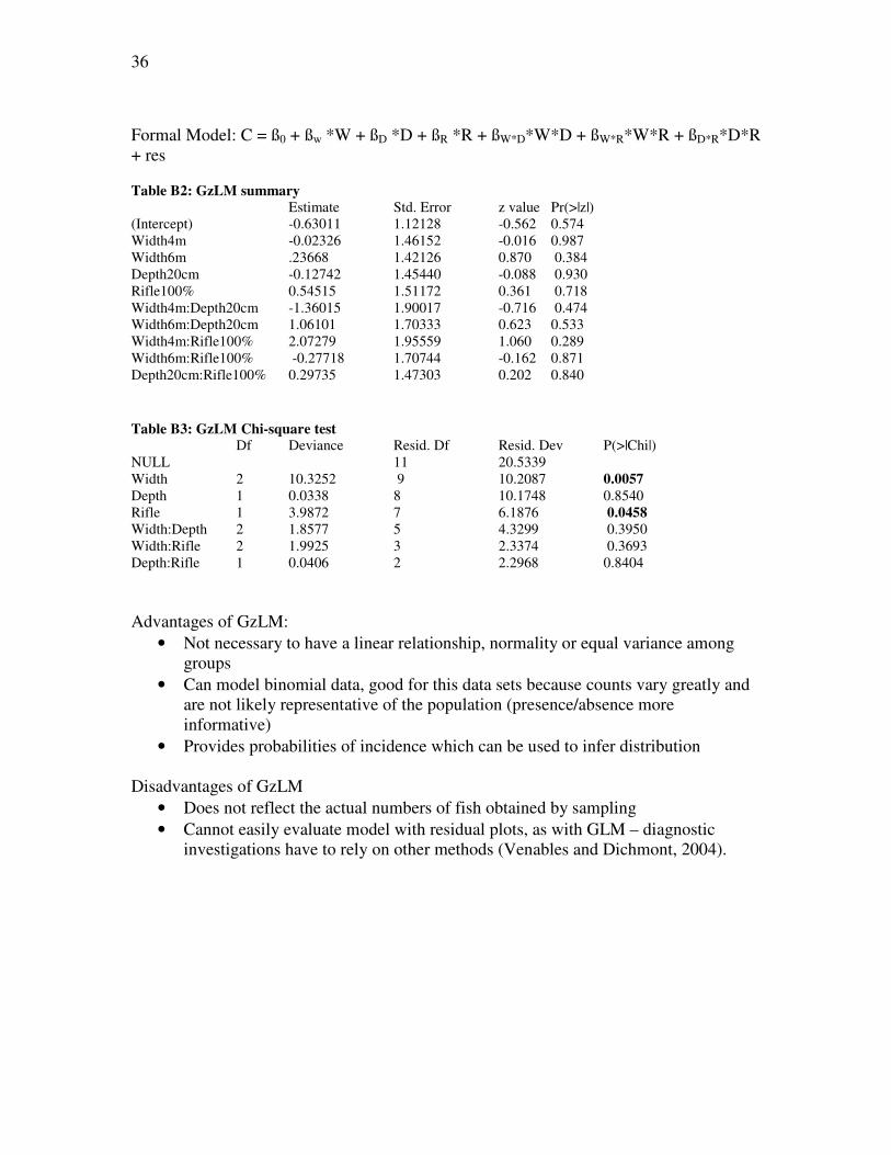
36

Formal Model: C = ß0 + ßw *W + ßD *D + ßR *R + ßW*D*W*D + ßW*R*W*R + ßD*R*D*R + res

Table B2: GzLM summary

Estimate Std. Error z value Pr(>|z|) (Intercept) -0.63011 1.12128 -0.562 0.574

Width4m -0.02326 1.46152 -0.016 0.987

Width6m .23668 1.42126 0.870 0.384

Depth20cm -0.12742 1.45440 -0.088 0.930

Rifle100% 0.54515 1.51172 0.361 0.718

Width4m:Depth20cm -1.36015 1.90017 -0.716 0.474 Width6m:Depth20cm 1.06101 1.70333 0.623 0.533

Width4m:Rifle100% 2.07279 1.95559 1.060 0.289

Width6m:Rifle100% -0.27718 1.70744 -0.162 0.871

Depth20cm:Rifle100% 0.29735 1.47303 0.202 0.840

Table B3: GzLM Chi-square test

Df Deviance Resid. Df Resid. Dev P(>|Chi|)

NULL 11 20.5339

Width 2 10.3252 9 10.2087 0.0057

Depth 1 0.0338 8 10.1748 0.8540

Rifle 1 3.9872 7 6.1876 0.0458 Width:Depth 2 1.8577 5 4.3299 0.3950

Width:Rifle 2 1.9925 3 2.3374 0.3693

Depth:Rifle 1 0.0406 2 2.2968 0.8404

Advantages of GzLM:

• Not necessary to have a linear relationship, normality or equal variance among groups

• Can model binomial data, good for this data sets because counts vary greatly and are not likely representative of the population (presence/absence more informative)

• Provides probabilities of incidence which can be used to infer distribution Disadvantages of GzLM

• Does not reflect the actual numbers of fish obtained by sampling

• Cannot easily evaluate model with residual plots, as with GLM – diagnostic investigations have to rely on other methods (Venables and Dichmont, 2004).

37

Appendix C

Age 1 Greenland Cod Counts

Suzanne Thompson

Research Question: Does the number of Greenland Cod (Gadus ogac) depend on amount of eelgrass at the site of sampling? Data: Counts of Age 1 Greenland Cod from beach seine tows at several sites conducted at Newman Sound, Terra Nova National Park. Seine tows were taken bi-weekly during from 2006 field season from May till November. Data was collected by the MUN Cod research group, and was retrieved from Bob Gregory at Department of Fisheries and Oceans. Model 1: General Linear Model Formal Model: N = ß0 + ßE*E + res Table C1: ANOVA

Sum Sq Df F value Pr(>F)

E 336.2 2 3.3667 0.03724

Residuals 7189.0 144

Model 2: Generalized Linear Model; error = Negative Binomial

Table C2: LR statistics for Type 1 Analysis

Source DF F-Value Chi-Square Pr>Chi-sq

E 2 2.75 5.50 0.0640

Table C3: LR statistics for Type 2 Analysis

Source DF F-Value Chi-Square Pr>Chi-Sq

E 2 0.00 7.54 0.0231

Advantages of GzLM:

• Negative Binomial distribution can deal with very over-dispersed abundance data, such is the case here, by adding an extra parameter.

• Shows slightly more sensitive test by giving a lower p-value for Type 2 analysis.

Disadvantages of GzLM:

• Extra parameter (dispersion) makes it difficult to interpret diagnostic tests (not shown) such as normal probability tests, and homogeneity.

38

Appendix D

Juvenile Fish Counts

Suzanne Thompson

Research Question: Does the number of juvenile fish depend on geology configuration of sea bed and time of day? Data: Counts of juvenile fish (mostly Haddock) from two 5 km transect lines on Western Bank of the Eastern Scotian Shelf. This data was collected by Tow Cam, a video camera which is towed from the back of a ship. Side scan sonar data was also collected of the sea bed configuration, classified in several categories, and matched up with camera data. Data was collected by Department of Fisheries and Oceans, and was retrieved from Bob Gregory. Model 1: General Linear Model Formal Model: N = ß0 + ßGeol*Geol + ßTime*Time + res Table D1: ANOVA

Source DF Type III SS Mean Square F Value Pr>F

Geol 7 48.4773 6.9253 42.72 <0.0001

Time 1 2.8739 2.8739 17.73 <0.0001

Model 2: Generalized Linear Model; error = Binomial

Table D2: LR statistics for Type 1 Analysis

Source Deviance DF Chi-Square Pr>ChiSq

Intercept 6180.1816

Geol 5860.7547 7 319.43 <0.0001

Time 5842.8680 1 17.89 <0.0001

Table D3: LR statistics for Type 2 Analysis

Source DF Chi-Square Pr>Chi-Square

Geol 7 308.19 <0.0001

Time 1 17.89 <0.0001

Advantages of GzLM:

• Because the data has many zeros, analysis can focus less on the abundance, and more on the probability of occurrence.

• Gives a good idea of the magnitude of the differences, because it is based on odds ratios and not on abundance data.

39

Appendix E Seed Removal Data

Andrew Trant

Research Question: Does seed removal by introduced red fire ant (Solenopsis invicta Burren) differ within or between plant species? Data: These data were collected in South Carolina, 1998. The study area was an abandoned field which had natural populations of the red fire ant. Cages were set up to exclude all known seed predators other than the red fire ant. At each ant mount, six cages were established with seeds placed within cages on platforms. The number of seeds removed was recorded every week for a total of six weeks. The following analysis uses the sums of seed removed over this entire period. These data were published by Seaman and Marino (2003). Model 1: General Linear Model; log transformed mean counts of seeds removed Formal Model: C = ß0 + ßS *S + ßM *M + res

Table E1: ANOVA

Df Sum Sq Mean Sq F-value Pr(>F) Species 4 32343 8086 18.111 9.273e-11

Mound 1 971 971 2.1746 0.1440

Residuals 84 37501 446

Table E2: General Linear Model Estimate Std. Error t-value Pr(>|t|)

(Intercept) 1.182 0.336 3.522 0.000696

SpeciesAmbrosia 0.649 0.372 1.746 0.084425 .

SpeciesChenopod -0.289 0.372 -0.778 0.438469

SpeciesPoa -1.145 0.372 -3.081 0.002788

SpeciesSolidago 0.403 0.372 1.084 0.281360 Mound -0.007 0.022 -0.318 0.751622

Model 2: Generalized Linear Model; error = Negative Binomial Table E3: GzLM summary

Estimate Std. Error t-value Pr(>|t|) (Intercept) 2.796 0.227 12.317 < 2e-16

SpeciesAmbrosia 1.277 0.248 5.154 1.66e-06

SpeciesChenopod 0.287 0.251 1.145 0.255

SpeciesPoa -0.271 0.254 -1.064 0.290

SpeciesSolidago 0.727 0.249 2.921 0.004

Mound 0.012 0.014 0.835 0.406

40

Table E4: GzLM Chi-square test Df Deviance Resid.Df ResidDev P(>|Chi|)

NULL 89 192.926

Species 4 53.141 85 139.786 1.774e-10

Mound 1 0.763 84 139.023 0.390

Advantages of GzLM:

• do not need to transform response variable to fit assumptions of normality

• unlike Poisson models that require and mean to variance ratio of 1, negative binomials models do

not

• greater sensitive to p-values compared to similar analysis with general linear model

Disadvantages of GzLM

• not ideal for small sample sizes

• requires estimate of additional parameter (theta)

Appendix F

Oak Recruitment Data

Andrew Trant

Research Question: Does the occurrence of fire and other measures of forest structure influence of the distribution of Red Oak (Quercus rubra)? Data: These data were collected November 2007 by Andrew Trant, Ian Morrison and Krista Chin in Kejimkujik National Park, NS as part of a study looking at the role of fire in regeneration and maintenance of Red Oak (Quercus rubra) stands. 20 plots were established within the boundary of Kejimkujik National Park in areas that with a known fire history. In each plot, demography and structural data were collected. These data are unpublished. Model 1: General Linear Model; log transformed mean seedling counts Formal Model: C = ß0 + ßF *F + ßBA *BA + ßDWD *DWD + res

Table F1: ANOVA

Df Sum Sq Mean Sq F-value Pr(>F)

fire 1 4.025 4.025 1.2219 0.2853 basal.area 1 10.512 10.512 3.1911 0.0930 .

dwdall 1 1.606 1.606 0.4876 0.4950

Residuals 16 52.709 3.294

Model 2: Generalized Linear Model; error = Negative Binomial Table F2: GzLM summary

Estimate Std. Error t-value Pr(>|t|)

(Intercept) -7.287 3.140 -2.320 0.034

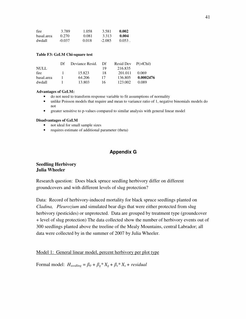
41

fire 3.789 1.058 3.581 0.002

basal.area 0.270 0.081 3.313 0.004

dwdall -0.037 0.018 -2.085 0.053 .

Table F3: GzLM Chi-square test

Df Deviance Resid. Df Resid Dev P(>|Chi|)

NULL 19 216.835 fire 1 15.823 18 201.011 0.069

basal.area 1 64.206 17 136.805 0.0002476

dwdall 1 13.803 16 123.002 0.089

Advantages of GzLM:

• do not need to transform response variable to fit assumptions of normality

• unlike Poisson models that require and mean to variance ratio of 1, negative binomials models do

not

• greater sensitive to p-values compared to similar analysis with general linear model

Disadvantages of GzLM

• not ideal for small sample sizes

• requires estimate of additional parameter (theta)

Appendix G

Seedling Herbivory

Julia Wheeler

Research question: Does black spruce seedling herbivory differ on different

groundcovers and with different levels of slug protection?

Data: Record of herbivory-induced mortality for black spruce seedlings planted on

Cladina, Pleurozium and simulated bear digs that were either protected from slug

herbivory (pesticides) or unprotected. Data are grouped by treatment type (groundcover

+ level of slug protection) The data collected show the number of herbivory events out of

300 seedlings planted above the treeline of the Mealy Mountains, central Labrador; all

data were collected by in the summer of 2007 by Julia Wheeler.

Model 1: General linear model, percent herbivory per plot type

Formal model: Hseedling = β0 + βg* Xg + βs* Xs + residual

42

Table G1: ANOVA

Source DF Seq SS Adj SS Adj MS F P

ground 2 0.050533 0.050533 0.025267 126.33 0.008

slug 1 0.018150 0.018150 0.018150 90.75 0.011

Error 2 0.000400 0.000400 0.000200 Total 5 0.069083

Model 2: Generalized linear model; error = binomial

Formal model: Odds (Hseedling) =e (Bref)

e (Bg)

e(Bs)

+ error

Table G2: GzLM summary

Standard Wald 95% Confidence Chi-

Parameter DF Estimate Error Limits Square P >ChiSq

Intercept 1 -0.8350 0.2413 -1.3080 -0.3621 11.97 0.0005

Groundcover L 1 -0.7580 0.3193 -1.3838 -0.1323 5.64 0.0176

Groundcover M 1 -1.2063 0.3501 -1.8926 -0.5200 11.87 0.0006

Slug O 1 0.6239 0.2740 0.0868 1.1610 5.18 0.0228

Scale 0 1.0000 0.0000 1.0000 1.0000

Table G3: GzLM Chi-square test

Source Deviance DF Square Pr > ChiSq

Intercept 19.5553

Groundcover 5.4940 2 14.06 0.0009 Slug 0.2048 1 5.29 0.0215

Advantages of GzLM:

• GzLM can consider interactive effects of groundcover and slug controls, while the

GLM has insufficient degrees of freedom (analysis performed, but not shown;

models above shows outputs when interactive effects are removed from both

models)

• Magnitude of the effect can be calculated using odds ratios derived from the

GzLM; GLM can only demonstrate a significant difference between herbivory

across treatments

• Provides lower p-value for groundcover, the variable of highest interest,

indicating a greater ability to detect an effect

Disadvantages of GzLM:

• Less sensitive than ANOVA for detecting effect for the second variable (level of

slug control)

43

Appendix H

Seed predation data

Julia Wheeler

Research question: Is conifer seed predation affected by substrate types and presence of

slug pesticides?

Data: Record of seed predation for black/white spruce seeds from 93 seed cards

distributed across Cladina, Pleurozium and simulated bear digs plots that were either

treated or untreated with slug pesticide. Data are grouped by treatment type. The cards

were collected and seed predation was determined by proportion of seeds removed (out

of 10 per card). Seed cards were distributed above the treeline of the Mealy Mountains in

central Labrador; all data were collected by in the summer of 2007 by Julia Wheeler.

Model 1: General linear model, percent seed predation per treatment type

Formal model: Hseed = β0 + βgroundcover* Xgroundcover + βslug* Xslug + residual

Table H1: ANOVA

Source DF Seq SS Adj SS Adj MS F P ground 2 0.041200 0.041200 0.020600 11.04 0.083

slug 1 0.004267 0.004267 0.004267 2.29 0.270

Error 2 0.003733 0.003733 0.001867

Total 5 0.049200

Model 2: Generalized linear model; error = binomial

Formal model: Odds (Hseed) =e (Bref)

e (Bgroundcover)

e(Bslug)

+ error

Table H2: GzLM summary

Standard Wald 95% Confidence Chi-

Parameter DF Estimate Error Limits Square Pr > ChiSq

Intercept 1 0.5379 0.1162 0.3102 0.7656 21.43 <.0001 Groundcover L 1 -0.5437 0.1622 -0.8616 -0.2257 11.23 0.0008

Groundcover M 1 -0.8252 0.1650 -1.1486 -0.5017 25.00 <.0001

Slug O 1 0.1719 0.1347 -0.0921 0.4360 1.63 0.2018

Scale 0 1.0000 0.0000 1.0000 1.0000

44

Table H3: GzLM Chi-square test

Chi-

Source Deviance DF Square Pr > ChiSq

Intercept 31.6419

Groundcover 3.8410 2 27.80 <.0001

Slug 2.2092 1 1.63 0.2015

Advantages of GzLM:

• Again, GzLM can consider interactive effects of groundcover and slug controls,

while the GLM has insufficient degrees of freedom

• Detects an effect from the groundcover parameter, where p-value is non-

significant using ANOVA

Disadvantages of GzLM:

• Residual plots are difficult to interpret for overdispersion

Appendix I

Avian Population Monitoring

Paul Regular

Research question: Do murre populations exhibit any long-term trends? Data: The following long-term count data was collected from census plots of common murres (Uria aalge) at Cape St. Mary’s, Newfoundland, 1980-2006 (Regular unpublished data) and thick-billed murres (Uria lomvia) at Coats Island, Nunavut, 1985-2000215. Murres were monitored using similar methods to the Type II approach described by Birkhead and Nettleship202. This technique has been adopted and routinely used to monitor common and thick-billed murre populations throughout the northern hemisphere. For the purposes of statistical analyses of these data, one may construct a GLM (linear regression) with the following formula: C = βo + βt*t + Normal error

Where C is the total number of murres attending plots on a particular day of the year when counts were conducted (response variable), and t represents the explanatory variable year.

Model 1: General linear model: Murre plot count data

45

Table I1: ANOVA for Cape St. Mary’s plot counts

Summary results

Estimate Standard error t-value P

(Intercept) -4271.8617 949.2923 -4.500 9.47e-06

T 2.2902 0.4776 4.796 2.47e-06

ANOVA table

df Sum of Squares Mean Sum of Squares F value P

T 1 51711 51711 22.997 2.5e-06

Residuals 326 733031 2249

Table I2: ANOVA for Coats Island plot counts

Summary results

Estimate Standard error t-value P

(Intercept) -72557.564 4398.959 -16.49 <2e-16

T 37.229 2.207 16.87 <2e-16

ANOVA table

df Sum of Squares Mean Sum of Squares F value P

T 1 14319562 14319562 284.56 <2.2e-16

Residuals 676 34017114 50321

Model 2: Generalized linear model; error = Poisson, negative binomial

Table I3: GzLM summary and Chi-square test for Cape St. Mary’s plot counts (error = Poisson)

Summary results

Estimate Standard error z-value P

(Intercept) -1.024e+01 1.169e+00 -8.756 <2e-16

T 7.987e-03 5.883e-04 13.577 <2e-16

Chi-square table

df Deviance Residual df Residual deviance P

NULL 327 2921.83

T 1 181.65 326 2740.18 2.116e-41

46

Table I4: GzLM summary and Chi-square test Parameter for Coats Island plot counts (error =

Poisson)

Summary results

Estimate Standard error z-value P

(Intercept) -3.788e+01 4.863e-01 -77.90 <2e-16

T 2.272e-02 2.439e-04 93.14 <2e-16

Chi-square table

df Deviance Residual df Residual deviance P

NULL 677 30659

T 1 8720 676 21939 0

Table I5: GzLM summary and Chi-square test for Cape St. Mary’s plot counts (error = negative

binomial)

Summary results

Estimate Standard error z-value P

(Intercept) -9.378271 3.551322 -2.641 0.00827

T 0.007553 0.001787 4.228 2.36e-05

Chi-square table

df Deviance Residual df Residual deviance P

NULL 327 353.04

T 1 19.13 326 333.91 1.222e-05

Table I6: GzLM summary and Chi-square test for Coats Island plot counts (error = negative

binomial)

Summary results

Estimate Standard error z-value P

(Intercept) -36.124955 2.885362 -12.52 <2e-16

T 0.021838 0.001448 15.09 <2e-16

Chi-square table

df Deviance Residual df Residual deviance P

NULL 677 918.76

T 1 236.03 676 682.73 2.884e-53

Table I7: GzLM summary and Chi-square test for Cape St. Mary’s plot counts (GAM)

Summary results

df n Deviance explained Chi-square P

s(t) 3 328 16.9% 512 <2e-16

47

Table I8: GzLM summary and Chi-square test Parameter for Coats Island plot counts (GAM)

Summary results

df n Deviance explained Chi-square P

s(t) 3 678 35.6% 11091 <2e-16

Advantages of GzLM:

• GzLM model does not assume a normal distribution and allows for non-linearity and non-constant variance structures in the data

• P-values generated by GzLM are lower, indicating stronger statistical power Disadvantages of GzLM

• GzLMs and GAMs include extra parameters to facilitate model fitting; data may be overfitted

Appendix J Bacterial abundance in ballast water and port water samples

Bei Sun

Research Question: If bacterial abundance depends on the two different water masses and pH?

Data: Sample were collected from both ship ballast tanks and receiving ports in three locations: Great Lakes, East Coast and West Coast of Canada. 10 ships from Great Lakes and 30 ships from west coast and east coast of Canada each were sampled from April to November, 2007. Several port samples were also collected in each location through the sampling season. Epi-fluorescent microscope direct count was used to investigate prokaryotical abundance. Physical parameters of those samples were recorded, named temperature, salinity and pH. The preliminary analysis indicated temperature and salinity were correlated, so samples were divided into two water masses by salinity 15‰. Model 1: General Linear Model

Formal model: εβββββ +•+•+•+= WpHpHWA pHWpHW0

Table J1: ANOVA

GLM Df Sum Sq Mean Sq F value Pr(>F)

Water masses 1 2.3286e+19 2.3286e+19 19.568 3.996e-05

pH 1 1.3086e+17 1.3086e+17 0.110 0.7413

Interaction 62 7.3779e+19 1.1900e+18

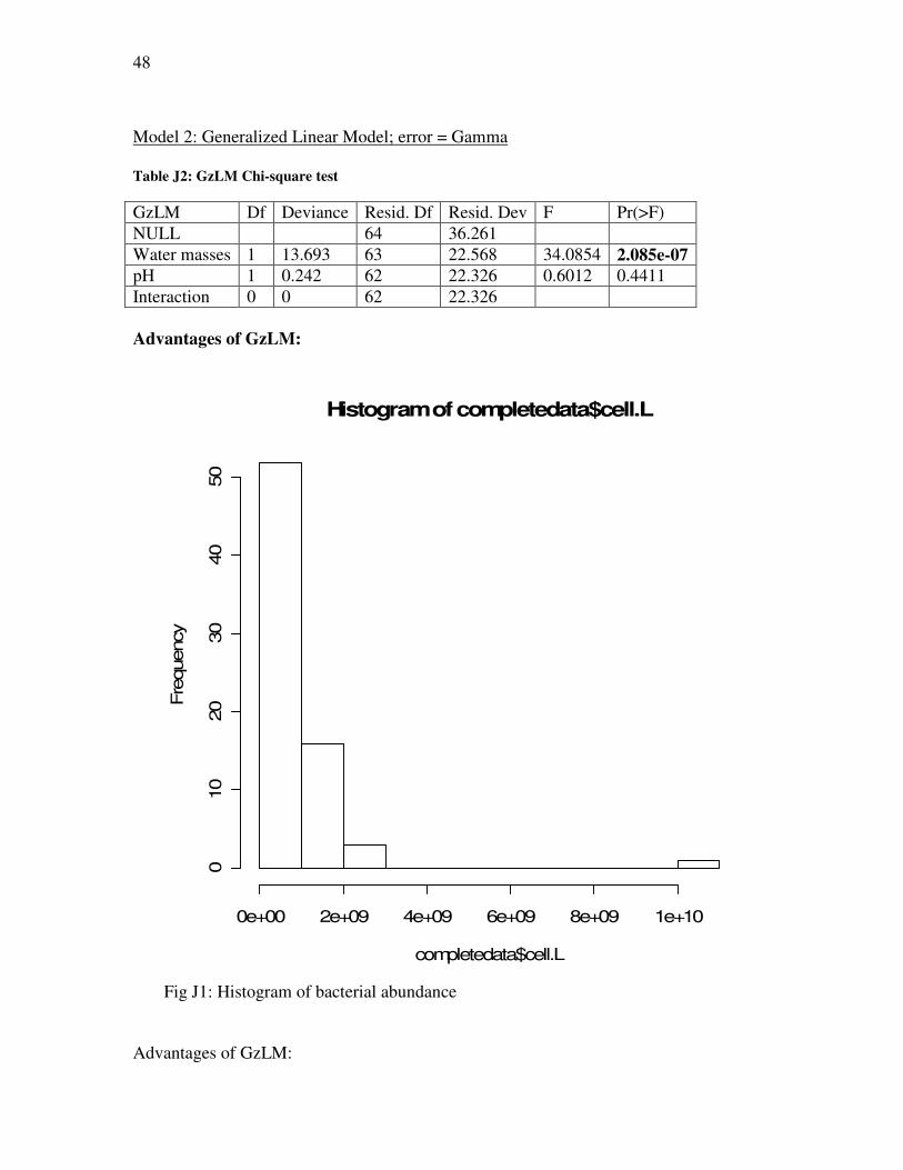
48

Model 2: Generalized Linear Model; error = Gamma

Table J2: GzLM Chi-square test

GzLM Df Deviance Resid. Df Resid. Dev F Pr(>F)

NULL 64 36.261

Water masses 1 13.693 63 22.568 34.0854 2.085e-07

pH 1 0.242 62 22.326 0.6012 0.4411

Interaction 0 0 62 22.326

Advantages of GzLM:

Histogram of completedata$cell.L

completedata$cell.L

Fre

quency

0e+00 2e+09 4e+09 6e+09 8e+09 1e+10

010

20

30

40

50

Fig J1: Histogram of bacterial abundance

Advantages of GzLM:

49

• Gamma can be applied to data with skewed distributions

• Application of the GzLM satisfies the assumption that the fits vs. residuals must be homogenous, and the assumption that the error points must be distributed along a normal line

Disadvantages of GzLM:

• Requires strong knowledge about advanced statistics

Appendix K

Bacterial colonies formed on different quadratic regions of different Petri dishes

Bei Sun Research Question: Is the number of bacterial colonies different on different quadratic regions of a series of Petri dishes? Data: We counted the number of bacteria colonies in 16 small quadratic regions of the same area in the central part of 5 different Petri dishes. Model 1: General Linear Model Formal Model: Two-way ANOVA

εβββ +•+•+= RPC rP0

Table K1: ANOVA

GLM Df Sum Sq Mean Sq F value Pr(>F)

Dishes 1 3.025 3.025 1.3580 0.2475

Quadratic 1 3.442 3.442 1.5454 0.2176

Residuals 77 171.520 2.228

Model 2: Generalized Linear Model; error = Poisson

Table K2: GzLM Chi-square test

GzLM Df Deviance Resid. Df Resid. Dev F Pr(>F)

NULL 79 76.092

Dishes 1 1.205 78 74.887 1.2048 0.2724

Quadratic 1 1.371 77 73.516 1.3711 0.2416

Advantages of GzLM:

• GzLM generates more accurate p-values since it represents the true distribution of the data

Disadvantages of GzLM:

• Requires strong knowledge about advanced statistics

50

Data set 2 from P395-396 Exercise 8.6 Chapter 8 The Poisson distribution. In Statistics with Applications in Biology and Geology. Preben Blasild, Jorgen Granfeldt (2003) Chapman & hall/CRC