general solution of the luneberg lens problem - … 29... · journal of applied physics volume 29....
TRANSCRIPT

General Solution of the Luneberg Lens ProblemSamuel P. Morgan Citation: J. Appl. Phys. 29, 1358 (1958); doi: 10.1063/1.1723441 View online: http://dx.doi.org/10.1063/1.1723441 View Table of Contents: http://jap.aip.org/resource/1/JAPIAU/v29/i9 Published by the American Institute of Physics. Additional information on J. Appl. Phys.Journal Homepage: http://jap.aip.org/ Journal Information: http://jap.aip.org/about/about_the_journal Top downloads: http://jap.aip.org/features/most_downloaded Information for Authors: http://jap.aip.org/authors
Downloaded 15 Apr 2012 to 193.136.128.7. Redistribution subject to AIP license or copyright; see http://jap.aip.org/about/rights_and_permissions
JOURNAL OF APPLIED PHYSICS VOLUME 29. NUMBER 9 SEPTEMBER. 1958
General Solution of the Luneberg Lens Problem
SAMUEL P. MORGAN
Bell Telephone Laboratories, Inc., Murray HUl, New Jersey (Received February 20, 1958)
The general solution is obtained for the index of refraction of a variable-index, spherical lens which will form perfect geometrical images of the points of two given concentric spheres on each other. One conjugate sphere is assumed to be outside the lens or at its surface, while the other may be either inside, outside or at the surface. If one of the spheres is of infinite radius, the lens will focus a parallel beam perfectly at ;, point on the other sphere.
It is shown that the in?ex of ~efraction may be specified arbitrarily, subject to two simple conditions, in an outer shell of any deSired thickness less than the radius of the lens. The index of the central portion is then expressed in terms of a function which is tabulated, and of an integral involving the index of the outer shell. Some properties of the general solution are discussed, and various special solutions are derived.
I. INTRODUCTION AND SUMMARY
A LUNEBERG lensl is a variable-index, spherically symmetric refracting structure which will form
perfect geometrical images of two given concentric spheres on each other. If one of the spheres is of infinite radius, the lens will focus a parallel beam of rays from any direction exactly at a point on the other sphere, or will form a perfectly parallel beam out of rays from a point source on the focal sphere. Recently considerable interest2- S has developed in microwave applications of Luneberg lenses, because of their obvious advantages as wide-angle scanners, and because of the possibility of simulating a variable index of refraction at microwave frequencies by means of artificial dielectrics.
The perfect focusing property of the Luneberg lens may be achieved in an infinite number of ways. Lunebergl found a particular solution for the index of refraction of a lens which has as conjugate foci two given points outside the lens. His solution takes a simple, explicit form if one of the points is at infinity and the other is at the surface of the lens. Subsequently Brown2
and Gutman3 have designed lenses with one focal point at infinity and the other inside the lens. None of these solutions is unique; and it turns out that in general, for arbitrarily chosen focal distances, the expression for the index of refraction involves functions defined by definite integrals, which have to be evaluated numerically.
The present paper derives the general expression for the index of refraction of a lens which will focus between two given conjugate points. One of the foci is taken to be outside the lens or at its surface; the other may be outside, inside, or at the surface. The only restriction on the solution is that the full aperture of the lens must be utilized; e.g., if it is desired to produce a parallel beam from a point source, the diameter of the beam must be equal to the diameter of the lens.
1 R. K. Luneberg, Mathematical Theory of Optics (Brown University, Providence, Rhode Island, 1944), pp. 189-213.
I J. Brown, Wireless Engineer 30, 250 (1953). a A. S. Gutman, J. Appl. Phys. 25, 855 (1954). 'Peeler, Kelleher, and Coleman, Inst. Radio Engrs. Trans.
AP-2, 94 (1954). 6 A. F. Kay, Inst. Radio Engrs. Trans. AP-4, 87 (1956). 8 K. S. Kelleher, Electronics 29, No.6, 138 (1956).
It is shown that the index of refraction may be specified arbitrarily, subject to two conditions, in an outer shell of any desired thickness less than the radius of the lens. The index of the central portion is then expressed in terms of a function which is tabulated in the appendix, and of an integral involving the index of the outer shell. The integration can sometimes be carried out explicitly, or it can be done numerically for any particular choice of index of the outer shell.
The paths of light rays in a radially symmetric refracting medium are discussed in Sec. II, and an integral equation is formulated which must be satisfied by the index of refraction of a Luneberg lens. A formal solution of the integral equation is obtained in Sec. III for a lens with two external foci, and in Sec. IV for a lens with one external and one internal focus. It is shown that if one wishes to design a lens, with two given external foci, in which the maximum index of refraction is as small as possible, the best design is the original Luneberg one. If on the other hand the criterion is that the variation in index shall be small, one can reduce the difference between maximum and minimum values appreciably by adjusting the index of the outer shell, at the expense of a very modest increase in the maximum index.
A simple relationship is derived in Sec. V between the illumination across the aperture of a large Luneberg lens antenna and the power pattern of a feed horn at the focal point. The result is independent of the particular distribution of index of refraction by which the perfect focusing property of the lens is achieved.
In Sec. VI the general theory is used to obtain various special solutions. In particular, the family of Luneberg lenses in which the index of refraction of the outer shell varies as any power of the radius is worked out completely in terms of the function tabulated in the appendix. A few illustrative numerical examples are given in Sec. VII.
II. MATHEMATICAL FORMULATION
Consider a medium in which the index of refraction n is a function only of the distance r from the origin. It
1358
Downloaded 15 Apr 2012 to 193.136.128.7. Redistribution subject to AIP license or copyright; see http://jap.aip.org/about/rights_and_permissions
G ENE R A L SOL UTI 0 N 0 F THE L UN E B ERG LEN S PRO B L E M 1359
follows from Fermat's principle that light rays in such a medium are plane curves which satisfy a generalization of Snell's law, namely
nr sin!p=K, (1)
where !p denotes the angle from the positive direction along the ray to the direction of increasing 1', and K is constant for a particular ray. This relationship is equivalent to the differential equation
n(r)r2dO/dr
[1+ (rdO/dr)2Jl (2)
where (1',0) are polar coordinates of points along the ray. Solving (2) for d(}/dr and integrating, we get
(3)
assuming that nCr) is a known function of r. The constant K and the ambiguous sign are determined by the direction of the ray at the initial point (1'0,00).
Since in the theory of radially symmetric media the index of refraction often occurs in the combination rn, it is convenient to introduce the notation
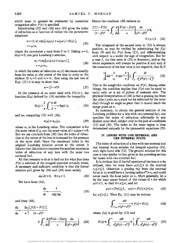
per) =rn(r). (4)
The medium is then equally well specified by the function per) or by the function nCr).
A point at which the distance of a particular ray from the origin is a maximum or minimum is called a "turning point" of the ray, and the coordinates of the turning point are denoted by (1'*,0*). Of course 1'* and 0* a're functions of the parameter K which characterizes the various rays. If nCr) is a continuous function, then
t " p -----------------~.-~-.~----.-----~
r a r-
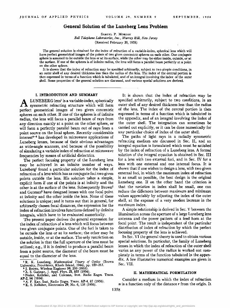
FIG. 1. A conceivable form of the function p (r) = rn (r).
(b)
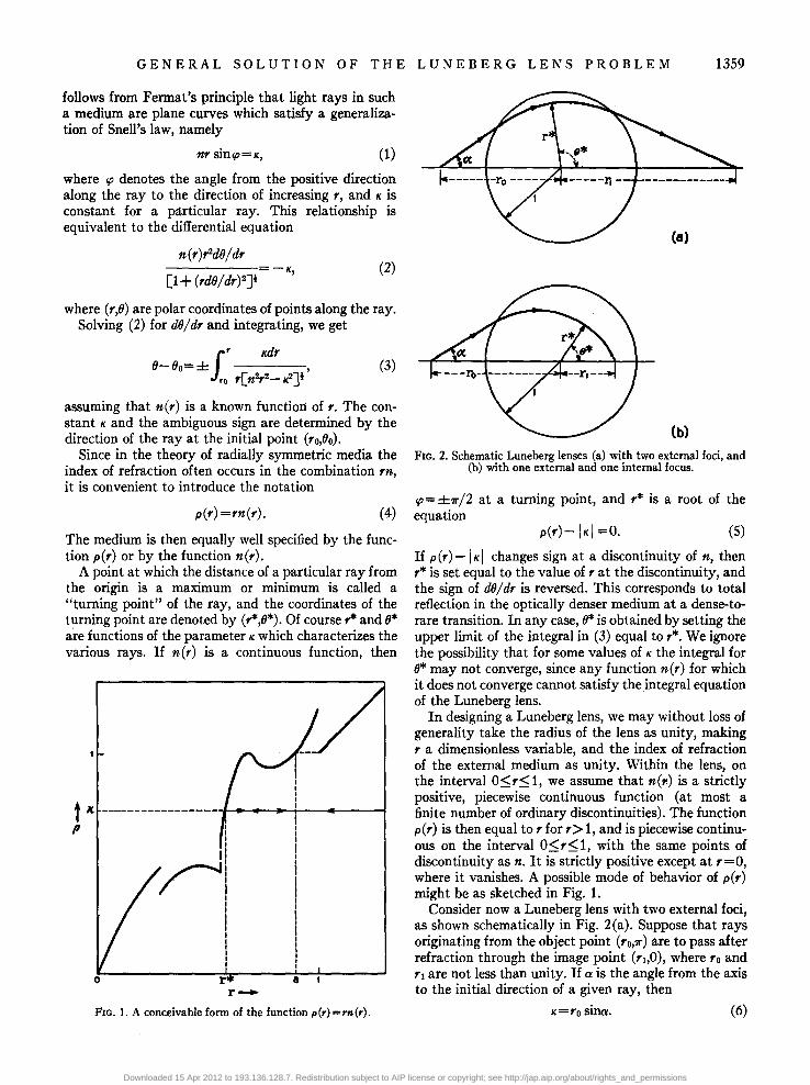
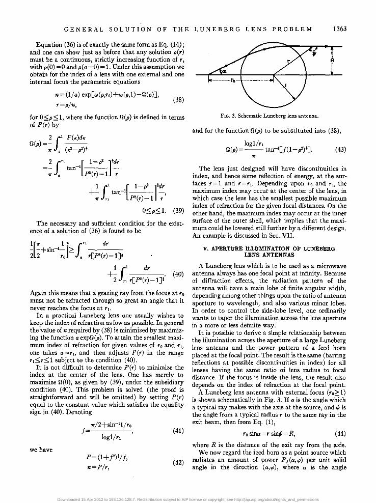
FIG. 2. Schematic Luneberg lenses (a) with two external foci, and (b) with one external and one internal focus.
!p=±'11/2 at a turning point, and r* is a root of the equation
(5)
If p(r)-IKI changes sign at a discontinuity of n, then r* is set equal to the value of r at the discontinuity, and the sign of d(} / dr is reversed. This corresponds to total reflection in the optically denser medium at a dense-torare transition. In any case, 0* is obtained by setting the upper limit of the integral in (3) equal to r*. We ignore the possibility that for some values of K the integral for 0* may not converge, since any function nCr) for which it does not converge cannot satisfy the integral equation of the Luneberg lens.
In designing a Luneberg lens, we may without loss of generality take the radius of the lens as unity, making r a dimensionless variable, and the index of refraction of the external medium as unity. Within the lens, on the interval O~r~l, we assume that n(1!) is a strictly positive, piecewise continuous function (at most a finite number of ordinary discontinuities). The function per) is then equal to r for r> 1, and is piecewise continuous on the interval 0~r~1, with the same points of discontinuity as n. It is strictly positive except at r=O, where it vanishes. A possible mode of behavior of per) might be as sketched in Fig. 1.
Consider now a Luneberg lens with two external foci, as shown schematically in Fig. 2(a). Suppose that rays originating from the object point (ro,'II'") are to pass after refraction through the image point (r1,0), where ro and r} are not less than unity. If a is the angle from the axis to the initial direction of a given ray, then
K=ro sina. (6)
Downloaded 15 Apr 2012 to 193.136.128.7. Redistribution subject to AIP license or copyright; see http://jap.aip.org/about/rights_and_permissions
1360 SAMUEL P. MORGAN
Since the radius of the lens is unity, it is easy to see that rays which meet the lens must have 0~1(:::;1.
Along a typical ray which starts from (ro,1I") with (J
and r both decreasing, the coordinate r continues to decrease until it first reaches a value r* for which p=K, or a discontinuity with P<K on the other side. To be precise, we define r*(K) in either case as the least upper bound of the set of r's for which per) <K. Note that r*(K) is a nondecreasing function of K, though it may have discontinuities and also intervals of constancy. Beyond the turning point r* the value of r increases with decreasing (J, and as the ray encounters no further turning points, it finally emerges from the lens and goes off to infinity. The situation for a particular value of K is indicated in Fig. 1.
The condition that every ray which starts from (rO,1I"), and meets the lens, is refracted so as to pass through (r1,0), may be written, using (3), in the form
0-11"= f:* r(p:~ ~)! f;1 r(p2~K2i (7)
The integral must be written in two parts because the ambiguous sign in (3) changes as the ray passes through the point (r*,O*). Integrating separately over the portions of path inside and outside the sphere and rearranging, we obtain the integral equation
where
II Kdr
f(K), O~K~l, r* (<<) r[p2(r) -~]t
(8)
(9)
and the inverse trigonometric functions are in the first quadrant.
This derivation does not consider rays which completely enciocle the origin.7 If each ray reaches the second focus after making N circuits of the origin, then a term N1I" must be added to the right side of (8). If all rays make the same number of circuits, Eq. (8) may be solved by the method of Sec. III; but the index of refraction becomes infinite at the center of the lens when N>O. If we assume that some but not all rays make complete circuits, the right side of (8) becomes dis~ontinuous in such a way that the equation has no solution.
The treatment of a Luneberg lens with one external and one internal focus is quite similar to the preceding. If the index of refraction is to remain finite everywhere, the focal points must lie on opposite sides of the center
7 R. Stettler, Optik 12, 529 (1955).
of the lens, so the configuration is as sketched in Fig. 2(b), withro~l andrl<1. The condition that a typical ray starting from (ro,1I") must pass through (rhO) takes the form
f T' Kdr iTt Kdr ----·+11"=0,
TO r(p2- ~)i T* r(p2- K2)! (10)
where it must be assumed (see Sec. IV) that the minimum radial distance r* is less than the focal distance r1.
On rearrangement, (10) becomes the fundamental integral equation for the Luneberg lens with one external and one internal focus, namely,
(11)
(12)
Ill. LENSES WITH TWO EXTERNAL FOCI
In this section we shall obtain the general solution of the integral equation (8) for a Luneberg lens with two external foci. We begin by discussing some general properties of the class of functions pCr) which can satisfy (8).
Our first observation is that the index of refraction nl at the lens surface cannot be less than unity if the full aperture of the lens is to be utilized. The reason for this is that a marginal ray which passes through the image point must be tangent to the lens in the external medium, and if nl<l such a ray would have been totally reflected before it ever entered the lens. It is easy to show that if a lens of unit radius, having nl~ 1, is to form a parallel beam from a point source, the radius of the beam will be just equal to nl. Hence for a full-aperture beam the function per) cannot be less than unity at the surface.
On the other hand, pC') may certainly be greater. than unity in the outer part of the lens. Suppose that
per) =P(r)~ 1, nCr) =P(r)/r~ l/r, (13)
for a~r~l, where a>O is the least upper bound of the values of r for which per) <1. The value of a is indicated in Fig. 1 for the particular variation of p shown there; it is evidently the distance of closest approach to the origin for the marginal ray. We shall see later what restrictions must he put on a and the function per) in order that Eq. (8) may possess a solution.
Assuming that the function per) is given in a~r~l, the function per) still has to be determined in O~r::;;a. Eq. (8) may now be written
fa Kdr
!(K)-F(K), 0:::;K~1, (14) r*(.) r[p2(r) - ~Jt
Downloaded 15 Apr 2012 to 193.136.128.7. Redistribution subject to AIP license or copyright; see http://jap.aip.org/about/rights_and_permissions
G ENE R A L SOL UTI 0 N 0 F THE L U NEB ERG LEN S PRO B L E M 1361
where j(K) is given by (9) and P(K) is defined as
II Kdr
F(K)= , 0~K~1, a r[F2(r)-K2]!
(15)
which will be a known function if per) is known. One can show in general that the solution of (14),
if it exists, is a continuous, strictly increasing function of r, with p(O) =0 and p(a-O) = 1. This means that per) can have no discontinuities, no maxima or minima, and no intervals of constancy in O<r<a.
To show that a discontinuity at r=R with p(R-O» p(R+O) is impossible (e.g., the left-hand discontinuity in Fig. 1), we observe that if such a discontinuity occurs at r=R, then the turning radius r*(K) is discontinuous at K=p(R+O). We may assume that p(R+O) <1, because otherwise per) must exhibit inadmissible behavior somewhere in the range R<r<a. Now the integrand in (8) is a positive function of rand a continuous function of K, so the value of the integral changes discontinuously as a function of K when the lower limit does. But j(K) is a continuous function of K in O~K~1; so the assumed discontinuity in per) cannot occur. An exactly similar argument eliminates the possibility that per) might have a local minimum or an interval of constancy in the range O<r<a.
If per) has a discontinuity at r=R with p(R-O)<p(R+O) (e.g., the middle discontinuity in Fig. 1), then by the definition of r*(K) we have r*(K) =R in the finite interval p(R-O) <K<p(R+O). The integral in (8) is obviously an increasing function of K if the limits are constant. But the right-hand side of (8) is easily shown by differentiation to be a decreasing function. Hence this type of discontinuity in per) is ruled out. The same argument applies if p(a-O)<1; hence we conclude that p(a-O) =1. That p(O) =0 follows from the definition of per) as rn(r) and the assumed boundedness of nCr).
Finally it follows from the definition of a that p(r)<1 for r slightly less than a, so per) cannot have a local maximum in O<r<a unless it also has a local minimum or a discontinuity in this range.
We now proceed to solve Eq. (14) on the assumption that per) is a continuous, strictly increasing function. Subsequently we shall establish a necessary and sufficient condition on per) in order that this may be true.
If p(r) is a continuous, strictly increasing function of r in the range O<r<a, then rep) is a continuous, strictly increasing function of p in the range O~p~ 1, and we may write
logr= -g(p), dr/r= -g'(p)dp, (16)
so that (14) becomes
f" K.g'(p)dp j(K)-F(K), O~K~1. (17) 1 (pL~)t
A simple change of variable reduces (17) to Abel's integral equation, the solution of which is known to
exist under very general conditions.8 The formal solution of (17) may be obtained directly, however, after replacing the dummy variable on the left by u, by multiplying both sides by dK/(K2-p2)i and integrating from p to 1. Interchanging the order of integration on the left, we obtain
(18)
or, in terms of r,
a 2 II j(K)dK 2 I1 F(K)dK log-=- , O~p~ 1. (19)
l' 7r p (K2_p2)! 7r p (K2_p2)!:
Following Luneberg,1 we introduce the function
1 II sin-1(K/s) w(p,s)=- dK, O~p~1, s2::1. (20)
7r p (K2_p2)t
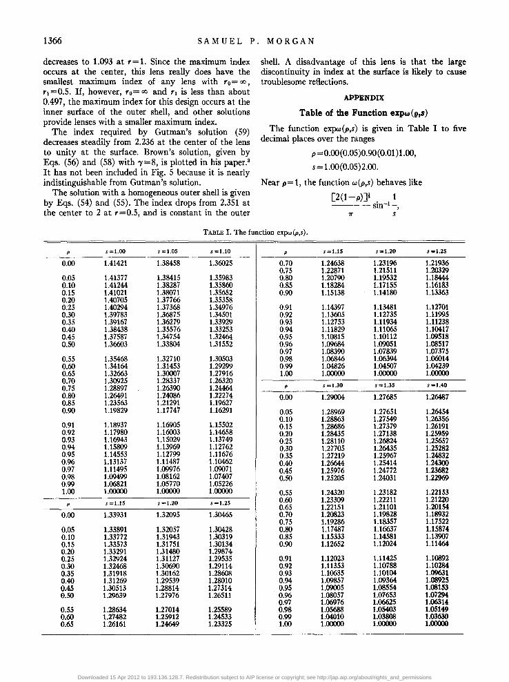
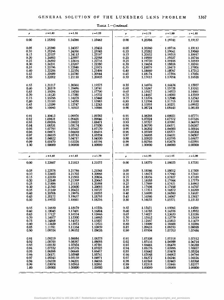
The function expw(p,s), which is what actually appears in the expression for the index of refraction, is tabulated in the appendix for 0~p~1, 1~s~2. Note in particular the values
1 JlI S sin-Ix w(O,s)=- --dx,
7r 0 x
w(1,s)=0,
w(p,1)=! log[1+(1-p2)t],
w(p,oo )=0.
Combining (9) and (20), we now have
2 II j(K)dK - w(p,ro)+w(p,rl)-Iogp, 7r p (KLp2)l
where use has been made of the result1
2 II COS-IK - dK= -logp. 7r p (K2- p2)!
Lastly, using (15), we define the function
2 II F(K)dK U(p)=-
7r p (K2-p2)1
(21)
(22)
(23)
=~ Jl tan-1[ 1-p2 ]tdr, (24) 7r a F2(r)-l r
8 G. Doetsch, Laplace-Transformation (Dover Publications, New York, 1943), pp. 293-294.
Downloaded 15 Apr 2012 to 193.136.128.7. Redistribution subject to AIP license or copyright; see http://jap.aip.org/about/rights_and_permissions
1362 SAMUEL P. MORGAN
which must in general be evaluated by numerical integration after Per) is specified.
Substituting (22) and (24) into (19) gives the index of refraction as a function of radius via the parametric equations
n= (l/a) exp[w(p,ro)+w(p,r1)-Q(p)],
r=p/n, (25)
where the parameter p runs from ° to 1. Taking a = 1, Q(p) =0, one gets Luneberg's solution,
nL=exp[w(p,ro)+w(p,r1)],
r=p/nL, (26)
in which the index of refraction nL(r) decreases steadily from its value at the center of the lens to unity at the surface. If 1'0= 1 and 1'1 = 00, then using the last two of Eqs. (21) it is easy to show that
n= (2-1'2)1. (27)
In the presence of an outer shell with P(r»l, the function Q(p) defined by (24) satisfies the inequality
2 f1 'If' dr Q(p)<- --=~ogl/a,
'If' a 2 r
and so, comparing (25) with (26),
n(p»nL(p),
(28)
(29)
where nL is the Luneberg value. The comparison is for the same value of p, not the same value of l' unless 1'=0.
But we can conclude from (29) that the index of refraction at the center of the lens is increased by the presence of the outer shell. Since the maximum index in the original Luneberg solution occurs at the center, it follows that this solution requires the smallest maximum index of refraction of any lens with the same two external foci.
All that remains to do is to find out for what functions Per) a solution of the integral equation actually exists. A necessary and sufficient condition is that the formal solution per) given by (16) and (18) must satisfy
dp/dr> 0, O<p<1. (30)
We have from (16),
dp 1 -=---, dr rdg/dp
(31)
and from (18),
dg = _ 2P{U(1)-F(1)]
dp 1/' (l-p2)t
+f1 ~[F(K)- J(")] dK }. (32) p dK K (~_p2)1
Hence the condition (30) reduces to
J(l) - F(l) f1 d [F(K) - J(")] dK ----+ - >0, (l-p2)i p dK K (K2_p2)1
O<p<1. (33)
The integrand of the second term in (33) is always positive, as may be verified by substituting for J(K) from (9) and for F(K) from (15), and differentiating with respect to K under the sign of integration. But for p near 1, the first term in (33) is dominant, and so the whole expression will always be positive if and only if the numerator of the first term is not negative, that is, if
~[sin-2..+sin-2..]> f1 dr . (34) 2 ro r1 - a r[P(r)-lJi
This is the sought-for condition on Per). Among other things, the condition implies that Per) can be equal to unity only on a set of points of measure zero. The physical interpretation of (34) is that a grazing ray from the object point at ro must not be refracted by the outer shell through an angle so great that it cannot reach the image point at 1'1.
In summary, to obtain the general solution of the Luneberg problem for a lens with two external foci, one specifies the index of refraction arbitrarily in any desired outer shell, subject only to the pair of conditions (13) and (34). The index in the inner region is then determined uniquely by the parametric equations (25).
IV. LENSES WITH ONE EXTERNAL AND ONE INTERNAL FOCUS
The index of refraction of a lens with one external and one internal focus satisfies the integral equation (11), with right-hand side (12). The general solution for this case is very similar to that given in the preceding section for lenses with two external foci.
It is obvious that if the full aperture of the lens is to be utilized, then we must havep(r)~l in the interval r1~ r~ 1. Otherwise a grazing ray from the external focus at ro would have a turning radius r*> r1, and could never reach the focal point at 1'1. More generally, let a be the least upper bound of the values of l' for which p(r)<l, so that O<a~r1, and let
per) =P(r)~ 1, nCr) =P(r)/r~ 1/1',
for a~r~1. Then Eq. (11) may be written
fa Kdr
f(K)-F(K), r*(.) r(p2- ~)i
where f(K) is given by (12) and
(35)
(36)
Jrl Kdr 1 f1 Kdr
F(K)= +- . (37) a r[p2(r)-~]l 2 rl r[p2(r)-~JI
Downloaded 15 Apr 2012 to 193.136.128.7. Redistribution subject to AIP license or copyright; see http://jap.aip.org/about/rights_and_permissions
G ENE R A L SOL UTI 0 N 0 F THE L U NEB ERG LEN S PRO B L E M 1363
Equation (36) is of exactly the same form as Eq. (14) j
and one can show just as before that any solution per) must be a continuous, strictly increasing function of 1', with p(O) =0 and p(a-O) = 1. Under this assumption we obtain for the index of a lens with one external and one internal focus the parametric equations
n= (l/a) exp[w(p,ro)+w(p,l)-Q(p)],
r=pln, (38)
for O:::;p:::;l, where the function Q(p) is defined in terms of Per) by
2 f r1 _ [ I-p2 ]idr =- tan I -
11" a P(r)-1 l'
+~ fl tan-if 1-p~lidr, 11" rt P(r)-1 l'
O:::;p:::;1. (39)
The necessary and sufficient condition for the existence of a solution of (36) is found to be
~[~+sin-~]> f" __ dr __ 2 2 1'0 - a r[P(r)-1]!
1 II dr +-2 "r[P(r)-li
(40)
Again this means that a grazing ray from the focus at 1'0
must not be refracted through so great an angle that it never reaches the focus at 1'1.
In a practical Luneberg lens one usually wishes to keep the index of refraction as low as possible. In general the value of n required by (38) is minimized by maximizing the function a expQ(p). To attain the smallest maximum index of refraction for given values of 1'0 and 1'1,
one takes a=rt, and then adjusts Per) in the range 1'1:::; 1':::; 1 subject to the condition (40).
It is not difficult to determine Per) to minimize the index at the center of the lens. One has merely to maximize Q(O), as given by (39), under the subsidiar'y condition (40). This problem is solved (the proof IS
straightforward and will be omitted) by setting Per) equal to the constant value which satisfies the equality sign in (40). Denoting
J
we have
11"/2 + sin-I l/ro
logl/rl
P= (1+ j2)i/J,
n=P/r,
(41)
(42)
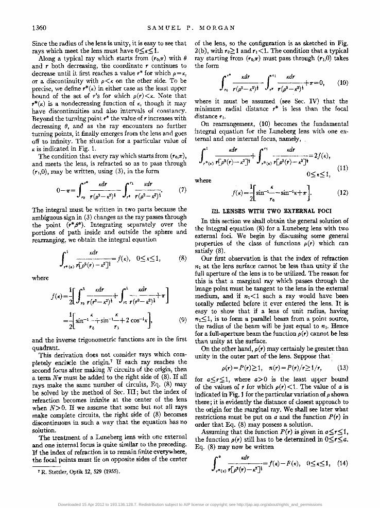
FIG. 3. Schematic Luneberg lens antenna.
and for the function Q(p) to be substituted into (38),
10gl/rl Q(p) =-- tan-I[j(I-p2)t]. (43)
The lens just designed will have discontinuities in index, and hence some reflection of energy, at the surfaces r= 1 and 1'=1'1. Depending upon 1'0 and 1'1, the maximum index may occur at the center of the lens, in which case the lens has the smallest possible maximum index of refraction for the given focal distances. On the other hand, the maximum index may occur at the inner surface of the outer shell, which implies that the maximum could be lowered still further by a different design. An example is discussed in Sec. VII.
V. APERTURE ILLUMINATION OF LUNEBERG LENS ANTENNAS
A Luneberg lens which is to be used as a microwave antenna always has one focal point at infinity. Because of diffraction effects, the radiation pattern of the antenna will have a main lobe of finite angular width, depending among other things upon the ratio of antenna aperture to wavelength, and also various minor lobes. In order to control the side-lobe level, one ordinarily wants to taper the illumination across the lens aperture in a more or less definite way.
It is possible to derive a simple relationship between the illumination across the aperture of a large Luneberg lens antenna and the power pattern of a feed horn placed at the focal point. The result is the same (barring reflections at possible discontinuities in index) for all lenses having the same ratio of lens radius to focal distance. If the focus is inside the lens, the result also depends on the index of refraction at the focal point.
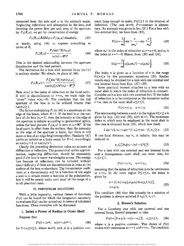
A Luneberg lens antenna with external focus (ro~ 1) is shown schematically in Fig. 3. If a is the angle which a typical ray makes with the axis at the source, and if; is the angle from a typical radius l' to the same ray in the exit beam, then from Eq. (1),
ro sina=r sinif;=R, (44)
where R is the distance of the exit ray from the axis. We now regard the feed horn as a point source which
radiates an amount of power P,(a,cp) per unit solid angle in the direction (a,cp), where a is the angle
Downloaded 15 Apr 2012 to 193.136.128.7. Redistribution subject to AIP license or copyright; see http://jap.aip.org/about/rights_and_permissions
1364 SAMUEL P. MORGAN
measured from the axis and cp is the aximuth angle. Neglecting reflections and absorption in the lens, and denoting the power flow per unit area of the aperture by Pa(R,cp), we get by conservation of energy
Pa(R,cp)RdRdcp=P/(a,cp) sinadadcp, (45)
or finally, using (44) to express everything in terms of R,
(46)
This is the desired relationship between the aperture illumination and the feed pattern.
The derivation for a lens with internal focus (1'0< 1) is entirely similar. We obtain, in place of (46),
Here nero) is the index of refraction at the focal point. If n(r) is discontinuous at 1'=1'0, we must take the "inner" value n(ro-O). The condition that the full aperture of the lens is to be utilized insures that ron(ro)~1.
The factor multiplying P / in (46) is a maximum at the edge of the beam, where R = 1. If the feed is at the surface of the lens (1'0= 1), then the intensity at the edge of the aperture is infinite according to geometrical optics, unless the feed pattern P,(a,cp) is zero at a=90°. If the focal point is offset from the surface, then the intensity at the edge of the aperture is finite, but there is still more or less of an edge-brightening effect. Similarly (47) yields an infinite or a finite result for R = 1, accordingly as ron (1'0) =1 or ron (1'0) > 1.
Clearly the preceding derivation takes no account of diffraction or reflection. The geometrical optics approximation, neglecting diffraction, should be reasonably good if the lens is many wavelengths across. The energy loss because of reflections can be included without much difficulty if there are discontinuities in index at the surface of the lens or elsewhere. The transmission coefficient at a discontinuity will be a function of the angle a and to a certain extent a function of the polarization, but it will be nearly unity over most of the range of a in all practical cases.
VI. PARTICULAR SOLUTIONS
With a little ingenuity, various classes of functions P(r) can be found for which the integration necessary to evaluate O(p) can be carried out in terms of tabulated functions. Three examples will be discussed.
1. Index a Power of Radius in Outer Shell
Suppose that
P(r)=Arm, n(r)=Arm-l, (48)
for O<a~r~ 1, where m~O, and A is a positive con-
stant large enough to make P(r)~1 in the interval of definition. (The case m=O, P=constant is elementary. An example was given in Sec. IV.) For a lens with two external foci, we have from (15),
(49)
where na+ is the index of refraction at r=a+O, and nl is the index at 1'=1-0. Hence, from (20) and (24),
O(p) = :r w(p,ana+) -w(p,nl) J (50)
The index n is given as a function of l' in the range O~r~a by the parametric equations (25). Similar results may be obtained for a lens with one external and one internal focus from Eqs. (37)-(39).
Some practical interest attaches to a lens with an outer shell in which the index of refraction is constant. Consider such a lens with two external foci. If the index of refraction is to be continuous at the transition radius r=a, then in the outer shell a~r~l,
P(r)=r/a, n=l/a. (51)
The relationship between nand l' in the region O~ r~ a is given by Eqs. (25) and (50), with m=1. The maximum index nl which may be employed in the outer shell in this case is bbtained from (34), which now reads
2 sin-l(l/nl)+sin-l(l/ro)+sin-l(l/rl)~l11". (52)
If one focal distance, say 1'1, is infinite, this may be reduced to
(53)
For a lens with one external and one internal focus and a homogeneous outer shell, one must take, for rl~r~ 1,
P(r) =1'/1'1, n=l/rl, (54)
assuming that the index of refraction is to be continuous at 1'=1'1. In the inner region O~r~rl, the index is given by
n= (1/1'1) exp[w(p,ro)+w(p,1/rl)],
r=p/n. (55)
The condition (40) that this actually be a solution of the problem is always satisfied if ro~l, 1'1<1.
2. Brown's Solution
For a Luneberg lens with one external and one internal focus, Brown2 proposed to take
P(r)=[1+,y(l-r)(r-rl)]i, rl~r~l, (56)
where 'Y is a positive constant. This choice of Per) makes nCr) continuous at 1'=1 and 1'=1'1. The condition
Downloaded 15 Apr 2012 to 193.136.128.7. Redistribution subject to AIP license or copyright; see http://jap.aip.org/about/rights_and_permissions
G ENE R A L SOL UTI 0 N 0 F THE L UN E B ERG LEN S PRO B L E M 1365
(40) becomes 1I'"/2+sin-1(1/ro);:::1I'"/('Yro)l. (57)
By ingenious analysis Brown evaluated the integral occurring in (39), which in the present notation reads
Using this expression for Q(p), the values of nand l' are given in 0::;1'::;1'1 by the parametric equations (38).
It is evident that a similar expression for Per) may be used, if desired, in a lens with two external foci.
3. Gutman's Solution
For a lens with an external focus at infinity and an internal focus at 1'1, Gutman3 found more or less by inspection the simple solution
nCr) = (1 +rI2-r2)!/rl' 0::;1'::; 1, (59)
which reduces to the Luneberg solution (27) if 1'1 = 1. In the present notation, this means
Per) =1'(1 +1'12_1'2)1/1'1, 1'1::;1'::; 1. (60) We have
II dr
r1 r[P(r)-lJl 2' (61)
so that the condition (40) is satisfied for all 1'0;::: 1. Making a change of variable in the definite integral which appears in (58), it may be shown that if Per) is given by (60), then
This result is to be substituted into the parametric equations (38). If 1'0= 00, the parameter p may be eliminated and we obtain the expression (59) for nCr).
1.6
I.!>
1.4
n 1.3
1.2
1.1
1.0
/ --- -- i --r-- .... / -~ .......
1--....... / - r-'- ~ ,
LUNEBERG SOLUT:;;""" r::::: l"'~ -- HOMOGENEOUS SHELL ........... ........ --- LINEAR-INDEX SHELL .......... - -
~ o 0.1 0.2 0.3 0.4 D.!> 0.6 0.7 0.8 0,9 1.0
r
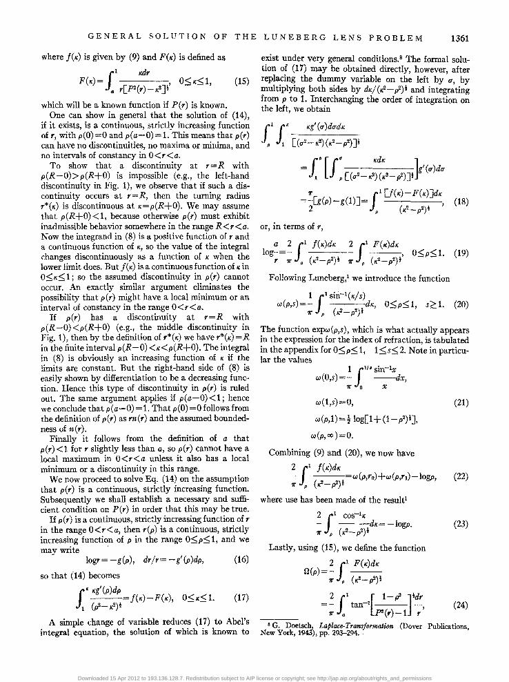
FIG. 4. Plots of index of refraction '/IS radius for three Luneberg lenses with 1'0= 1.1 and 1'1 = 00.
2.4
2.2
2.0
1.8
n 1.6
1.4
1.2
1.0
-r-- r---, -~ ~ 1\ ~ t--,
\(' ~. MINIMUM-INDEX ~ >~ I--- - - GUTMAN SOLUTION
--- HOMOGENEOUS SHELL
" ~" " D 0.1 0.2 0.3 0.4 D.!> 0.6 0.1 0.8 0.9 1.0 r
FIG. 5. Plots of index of refraction '/IS radius for three Luneberg lenses with 1'0= 00 and 1'1=0.5.
Gutman's solution cannot be adapted to a lens with two external foci, because in view of (61) the condition (34) is impossible unless 1'0=1'1 = 1.
VII. NUMERICAL EXAMPLES
As examples of lenses with two external foci, we have computed from the formulas of Sec. VI-1 three different lenses all having 1'0=1.1,1'1= 00. These are:
(a) Original Luneberg solution; (b) Homogeneous outer shell with n=1.15 for
0.8696::; 1'::; 1 ; (c) Outer shell with n=1.6r for 0.7906::;1'::;1.
The transition radius was chosen in cases (b) and (c) to make the index of refraction continuous there. The index is plotted against radius in Fig. 4.
In the Luneberg solution, the index of refraction decreases from 1.360 at the center of the lens to 1 at the surface. The introduction of a homogeneous outer shell of index 1.15 raises the index at the center only to 1.403, and thus appreciably decreases the range of variation of n. For this particular lens we could according to (53) have used an outer shell with nl as high as 1.188, in which case the center value would have been 1.419.
The third example, in which n = 1.6r in the outer shell, is largely of academic interest. It represents a lens which does not have its maximum index at the center.
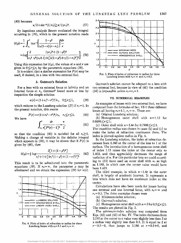
Calculations have also been made for lenses having one external and one internal focus, with 1'0= 00 and 1'1 = 0.5. The three examples chosen were
(a) Minimum-index solution; (b) Gutman's solution; (c) Homogeneous outer shell with n=2 for 0.5::;1'::; 1.
The results are plotted in Fig. 5. The minimum-index solution was computed from
Eqs. (42) and (43) of Sec. IV. The index decreases from 2.192 at the center to a value very slightly less than 2 at a radius very slightly less than 0.5. It is equal to 2 at 1'=0.5-0, then jumps to 2.186 at 1'=0.5+0, and
Downloaded 15 Apr 2012 to 193.136.128.7. Redistribution subject to AIP license or copyright; see http://jap.aip.org/about/rights_and_permissions
1366 SAM UEL P. MORGAN
decreases to 1.093 at ,=1. Since the maximum index shell. A disadvantage of this lens is that the large occurs at the center, this lens really does have the discontinuity in index at the surface is likely to cause smallest maximum index of any lens with '0= 00, troublesome reflections. '1 =0.5. If, however, '0= 00 and '1 is less than about
APPENDIX 0.497, the maximum index for this design occurs at the inner surface of the outer shell, and other solutions Table of the Function expw(p,s) provide lenses with a smaller maximum index.
The function expw(p,s) is given in Table I to five The index required by Gutman's solution (59) decreases steadily from 2.236 at the center of the lens decimal places over the ranges
to unity at the surface. Brown's solution, given by p=0.00(0.05)0.90(O.01)1.00, Eqs. (56) and (58) with ,),=8, is plotted in his paper.3 s = 1.00(0.05)2.00. It has not been included in Fig. 5 because it is nearly indistinguishable from Gutman's solution. Near p = 1, the function w (p,s) behaves like
The solution with a homogeneous outer shell is given [2(1-p)Ji 1 by Eqs. (54) and (55). The index drops from 2.351 at sin-1 -,
the center to 2 at ,=0.5, and is constant in the outer 7r s
TABLE 1. The function expw(p,s).
p s=l.oo s =1.05 s =1.10 p s=1.15 5-1.20 5-1.25
0.00 1.41421 1.38458 1.36025 0.70 1.24638 1.23196 1.21936 0.75 1.22871 1.21511 1.20329
0.05 1.41377 1.38415 1.35983 0.80 1.20790 1.19532 1.18444 0.10 1.41244 1.38287 1.35860 0.85 1.18284 1.17155 1.16183 0.15 1.41021 1.38071 1.35652 0.90 1.15138 1.14180 1.13363 0.20 1.40705 1.37766 1.35358 0.25 1.40294 1.37368 1.34976 0.91 1.14397 1.13481 1.12701 0.30 1.39783 1.36875 1.34501 0.92 1.13605 1.12735 1.11995 0.35 1.39167 1.36279 1.33929 0.93 1.12753 1.11934 1.11238 0.40 1.38438 1.35576 1.33253 0.94 1.11829 1.11065 1.10417 0.45 1.37587 1.34754 1.32464 0.95 1.10815 1.10112 1.09518 0.50 1.36603 1.33804 1.31552 0.96 1.09684 1.09051 1.08517
0.97 1.08390 1.07839 1.07375 0.55 1.35468 1.32710 1.30503 0.98 1.06846 1.06394 1.06014 0.60 1.34164 1.31453 1.29299 0.99 1.04826 1.04507 1.04239 0.65 1.32663 1.30007 1.27916 1.00 1.00000 1.00000 1.00000 0.70 1.30925 1.28337 1.26320
s =1.30 s =1.35 s -1.40 0.75 1.28897 1.26390 1.24464 p
0.80 1.26491 1.24086 0.85 1.23563 1.21291
1.22274 0.00 1.19627
1.29004 1.27685 1.26487
0.90 1.19829 1.17747 1.16291 0.05 1.28969 1.27651 1.26454 0.10 1.28863 1.27549 1.26356
0.91 1.18937 1.16905 1.15502 0.15 1.28686 1.27379 1.26191 0.92 1.17980 1.16003 1.14658 0.20 1.28435 1.27138 1.25959 0.93 1.16943 1.15029 1.13749 0.25 1.28110 1.26824 1.25657 0.94 1.15809 1.13969 1.12762 0.30 1.27705 1.26435 1.25282 0.95 1.14553 1.12799 1.11676 0.35 1.27219 1.25967 1.24832 0.96 1.13137 1.11487 1.10462 0.40 1.26644 1.25414 1.24300 0.97 1.11495 1.09976 1.09071 0.45 1.25976 1.24772 1.23682 0.98 1.09499 1.08162 1.07407 0.50 1.25205 1.24031 1.22969 0.99 1.06821 1.05770 1.05226 1.00 1.00000 1.00000 1.00000 0.55 1.24320 1.23182 1.22153
s =1.15 s =1.20 s =1.25 0.60 1.23309 1.22211 1.21220 0.65 1.22151 1.21101 1.20154
0.00 1.33931 1.32095 1.30465 0.70 1.20823 1.19828 1.18932 0.75 1.19286 1.18357 1.17522
0.05 1.33891 1.32057 1.30428 0.80 1.17487 1.16637 1.15874 0.10 1.33772 1.31943 1.30319 0.85 1.15333 1.14581 1.13907 0.15 1.33573 1.31751 1.30134 0.90 1.12652 1.12024 1.11464 0.20 1.33291 1.31480 1.29874 0.25 1.32924 1.31127 1.29535 0.91 1.12023 1.11425 1.10892 0.30 1.32468 1.30690 1.29114 0.92 1.11353 1.10788 1.10284 0.35 1.31918 1.30162 1.28608 0.93 1.10635 1.10104 1.09631 0.40 1.31269 1.29539 1.28010 0.94 1.09857 1.09364 1.08925 0.45 1.30513 1.28814 1.27314 0.95 1.09005 1.08554 1.081S3 0.50 1.29639 1.27976 1.26511 0.96 1.08057 1.07653 1.07294
0.97 1.06976 1.06625 1.06314 0.55 1.28634 1.27014 1.25589 0.98 1.05688 1.05403 1.05149 0.60 1.27482 1.25912 1.24533 0.99 1.04010 1.03808 1.03630 0.65 1.26161 1.24649 1.23325 1.00 1.00000 1.00000 1.00000
Downloaded 15 Apr 2012 to 193.136.128.7. Redistribution subject to AIP license or copyright; see http://jap.aip.org/about/rights_and_permissions
GENERAL SOLUTION OF THE LUNEBERG LENS PROBLEM 1367
TABLE r.-Continued.
s =1.45 s=1.50 s -1.55 p s=1.75 s=I.80 s =1.85
0.00 1.25392 1.24388 1.23462 0.00 1.20386 1.19741 1.19137
0.05 1.25360 1.24357 1.23433 0.05 1.20360 1.19716 1.19113 0.10 1.25266 1.24266 1.23345 0.10 1.20282 1.19641 1.19040 0.15 1.25107 1.24113 1.23197 0.15 1.20152 1.19515 1.18917 0.20 1.24883 1.23897 1.22988 0.20 1.19969 1.19337 1.18744 0.25 1.24592 1.23616 1.22716 0.25 1.19730 1.19105 1.18519 0.30 1.24231 1.23267 1.22380 0.30 1.19434 1.18818 1.18241 0.35 1.23796 1.22848 1.21975 0.35 1.19079 1.18473 1.17906 0.40 1.23284 1.22354 1.21498 0.40 1.18660 1.18067 1.17512 0.45 1.22689 1.21780 1.20944 0.45 1.18174 1.17596 1.17054 0.50 1.22002 1.21118 1.20305 0.50 1.17615 1.17054 1.16528
0.55 1.21217 1.20361 1.19575 0.55 1.16976 1.16434 1.15927 0.60 1.20319 1.19496 1.18741 0.60 1.16247 1.15728 1.15241 0.65 1.19294 1.18510 1.17790 0.65 1.15417 1.14923 1.14461 0.70 1.18120 1.17380 1.16702 0.70 1.14467 1.14003 1.13569 0.75 1.16766 1.16078 1.15448 0.75 1.13376 1.12946 1.12543 0.80 1.15185 1.14558 1.13985 0.80 1.12104 1.11715 1.11350 0.85 1.13299 1.12747 1.12243 0.85 1.10593 1.10251 1.09932 0.90 1.10960 1.10503 1.10086 0.90 1.08724 1.08443 1.08180
0.91 1.10413 1.09978 1.09582 0.91 1.08288 1.08021 1.07771 0.92 1.09831 1.09420 1.09046 0.92 1.07824 1.07572 1.07336 0.93 1.09206 1.08822 1.08471 0.93 1.07327 1.07091 1.06870 0.94 1.08531 1.08174 1.07850 0.94 1.06790 1.06571 1.06367 0.95 1.07793 1.07467 1.07170 0.95 1.06202 1.06003 1.05816 0.96 1.06971 1.06680 1.06414 0.96 1.05549 1.05371 1.05204 0.97 1.06035 1.05783 1.05554 0.97 1.04805 1.04651 1.04507 0.98 1.04922 1.04717 1.04530 0.98 1.03920 1.03795 1.03677 0.99 1.03470 1.03326 1.03194 0.99 1.02766 1.02678 1.02595 1.00 1.00000 1.00000 1.00000 1.00 1.00000 1.00000 1.00000
p s =1.60 s =1.65 s=1.70 p s =1.90 s =1.95 s=2.oo
0.00 1.22607 1.21813 1.21075 0.00 1.18570 1.18035 1.17531
0.05 1.22578 1.21786 1.21048 0.05 1.18546 1.18012 1.17509 0.10 1.22493 1.21703 1.20968 0.10 1.18475 1.17943 1.17441 0.15 1.22350 1.21565 1.20834 0.15 1.18356 1.17827 1.17329 0.20 1.22148 1.21369 1.20645 0.20 1.18188 1.17664 1.17170 0.25 1.21886 1.21115 1.20398 0.25 1.17969 1.17451 1.16963 0.30 1.21560 1.20800 1.20093 0.30 1.17698 1.17188 1.16707 0.35 1.21169 1.20422 1.19727 0.35 1.17373 1.16872 1.16399 0.40 1.20708 1.19976 1.19295 0.40 1.16990 1.16500 1.16037 0.45 1.20172 1.19457 1.18793 0.45 1.16546 1.16067 1.15617 0.50 1.19555 1.18861 1.18216 0.50 1.16035 1.15571 1.15133
0.55 L18850 1.18179 1.17556 0.55 1.15451 1.15003 1.14581 0.60 1.18045 1.17401 1.16804 0.60 1.14785 1.14356 1.13952 0.65 1.17127 1.16514 1.15946 0.65 1.14027 1.13620 1.13236 0.70 1.16077 1.15500 1.14965 0.70 1.13162 1.12779 1.12419 0.75 1.14868 1.14333 1.13837 0.75 1.12167 1.11813 1.11479 0.80 1.13459 1.12973 1.12523 0.80 1.11009 1.10688 1.10386 0.85 1.11781 1.11354 1.10959 0.85 1.09633 1.09353 1.09088 0.90 1.09704 1.09352 1.09026 0.90 1.07934 1.07703 1.07486
0.91 1.09219 1.08884 1.08575 0.91 1.07538 1.07318 1.07112 0.92 1.08703 1.08387 1.08095 0.92 1.07116 1.06909 1.06714 0.93 1.08150 1.07854 1.07581 0.93 1.06664 1.06470 1.06288 0.94 1.07552 1.07278 1.07025 0.94 1.06176 1.05996 1.05827 0.95 1.06898 1.06648 1.06417 0.95 1.05642 1.05478 1.05324 0.96 1.06171 1.05948 1.05741 0.96 1.05048 1.04902 1.04764 0.97 1.05343 1.05150 1.04971 0.97 1.04372 1.04246 1.04126 0.98 1.04358 1.04201 1.04055 0.98 1.03568 1.03465 1.03368 0.99 1.03074 1.02963 1.02861 0.99 1.02518 1.02446 1.02377 1.00 1.00000 1.00000 1.00000 1.00 1.00000 1.00000 1.00000
Downloaded 15 Apr 2012 to 193.136.128.7. Redistribution subject to AIP license or copyright; see http://jap.aip.org/about/rights_and_permissions
1368 SAMUEL P. MORGAN
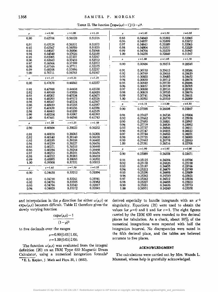
TABLE II. The function [expw(p,s)-1J/(1-p)l.
s=1.00 s =1.05 s =1.10 p s =1.45 s=1.50 s -1.55
0.90 0.62704 0.56120 0.51516 0.95 0.34849 0.33392 0.32065 0.96 0.34857 0.33399 0.32072
0.91 0.63124 0.56351 0.51673 0.97 0.34845 0.33389 0.32063 0.92 0.63567 0.56580 0.51825 0.98 0.34804 0.33351 0.32029 0.93 0.64037 0.56806 0.51968 0.99 0.34704 0.33259 0.31945 0.94 0.64540 0.57026 0.52100 1.00 0.34258 0.32849 0.31567 0.95 0.65085 0.57237 0.52217
s=1.65 0.96 0.65685 0.57433 0.52312 s=1.60 s=1.70
0.97 0.66364 0.57599 0.52372 0.90 0.30686 0.29573 0.28543 0.98 0.67166 0.57711 0.52375 0.99 0.68208 0.57696 0.52257 0.91 0.30730 0.29615 0.28584 1.00 0.70711 0.56763 0.51367 0.92 0.30769 0.29653 0.28620
s =1.15 s =1.20 s =1.25 0.93 0.30803 0.29685 0.28652 0.94 0.30830 0.29712 0.28678
0.90 0.47870 0.44842 0.42257 0.95 0.30849 0.29730 0.28696 0.96 0.30857 0.29739 0.28705
0.91 0.47988 0.44938 0.42338 0.97 0.30850 0.29733 0.28701 0.92 0.48100 0.45026 0.42410 0.98 0.30818 0.29705 0.28676 0.93 0.48202 0.45104 0.42475 0.99 0.30741 0.29634 0.28611 0.94 0.48293 0.45172 0.42528 1.00 0.30392 0.29310 0.28309 0.95 0.48367 0.45224 0.42567 0.96 0.48419 0.45255 0.42587 p s =1.75 s =1.80 s -1.85
0.97 0.48439 0.45256 0.42580 0.90 0.27588 0.26698 0.25867 0.98 0.48405 0.45209 0.42529 0.99 0.48264 0.45067 0.42393 0.91 0.27627 0.26736 0.25904 1.00 0.47461 0.44346 0.41743 0.92 0.27662 0.26770 0.25938
s =1.30 s =1.35 s =1.40 0.93 0.27693 0.26801 0.25967 0.94 0.27719 0.26826 0.25992
0.90 0.40008 0.38023 0.36252 0.95 0.27737 0.26844 0.26011 0.96 0.27747 0.26855 0.26022
0.91 0.40078 0.38085 0.36308 0.97 0.27744 0.26853 0.26021 0.92 0.40140 0.38140 0.36358 0.98 0.27721 0.26833 0.26003 0.93 0.40195 0.38188 0.36402 0.99 0.27662 0.26778 0.25953 0.94 0.40239 0.38227 0.36436 1.00 0.27381 0.26516 0.25708 0.95 0.40271 0.38253 0.36460
s =1.95 0.96 0.40284 0.38264 0.36468 s =1.90 $=2.00
0.97 0.40273 0.38251 0.36456 0.90 0.25089 0.24358 0.23671 0.98 0.40222 0.38203 0.36410 0.99 0.40095 0.38085 0.36302 0.91 0.25125 0.24394 0.23706 1.00 0.39508 0.37551 0.35815 0.92 0.25158 0.24426 0.23738
s =1.45 s =1.50 s=1.55 0.93 0.25187 0.24455 0.23766 p
0.94 0.25212 0.24479 0.23790 0.90 0.34658 0.33212 0.31894 0.95 0.25230 0.24498 0.23809
0.96 0.25242 0.24510 0.23821 0.91 0.34710 0.33261 0.31941 0.97 0.25242 0.24512 0.23824 0.92 0.34756 0.33305 0.31982 0.98 0.25227 0.24498 0.23813 0.93 0.34796 0.33342 0.32017 0.99 0.25181 0.24456 0.23773 0.94 0.34828 0.33372 0.32045 1.00 0.24951 0.24240 0.23570
and interpolation in the p direction for either w(p,s) or derived especially to handle integrands with an x-I expw(p,s) becomes difficult. Table II therefore gives the singularity. Equations (21) were used to obtain the slowly varying function values for p=O and 1 and for s=1. The eight figures
expw(p,s)-l carried by the IBM 650 were rounded to five decimal
(l-p)t places for tabulation. As a check, about 10% of the numerical integrations were repeated with half the
to five decimals over the ranges integration interval. No discrepancies were noted in
p=0.90(0.01)1.00, the fifth decimal place, and the tables are believed
s = 1.00 (0.05) 2.00. accurate to five places.
The function w(p,s) was evaluated from the integral ACKNOWLEDGMENT definition (20) on an IBM Type 650 Magnetic Drum
Calculator, using a numerical integration formula9 The calculations were carried out by Mrs. Wanda L. e E. L. Kaplan, J. Math and Phys. 31, 1 (1952). Mammel, whose help is gratefully acknowledged.
Downloaded 15 Apr 2012 to 193.136.128.7. Redistribution subject to AIP license or copyright; see http://jap.aip.org/about/rights_and_permissions