general laboratory instructionrh23-06 · return the signed proclamation form to the departmental...

Physical Chemistry General Instruction

Chemistry Department University of Malaya

1

Suitable for courses SCES1230, SCES2230, SCES3130 1. General Safety and Laboratory Instruction

a. Before entering any chemistry laboratory, make sure you have a copy of the safety handbook from the Department office. You must sign a proclamation form as a proof that you have read and understood the content of the safety handbook. Please return the signed proclamation form to the Departmental Office. Failure to do this may prohibit you to enter the laboratory or you may lose the right of protection should accident occur.

b. Common safety practice and guidelines MUST be obeyed at all time when you are

in the laboratory. Please refer to the safety handbook regularly. When unsure on any matter related to safety, seek help from the lecturer-in-charge.

c. In the laboratory, you MUST wear proper attire i.e. laboratory coat and safety

glasses.

d. When handling any chemical, please make sure you have read its MSDS Material Safety Data Sheet. (for information see for example http://www.ilpi.com/msds/#What).

e. DO NOT dispose mercury into the sink. Mercury is expensive, toxic and poisonous.

Used and contaminated mercury must be transferred into the residue bottle which is provided. Any spillage of mercury MUST be reported to the lab assistant.

f. DO NOT dispose of organic solvent into the sink. Any used organic solvent must be

transferred into the appropriately labeled waste bottles. Please consult the lab assistant if you are uncertain.

g. When dealing with compressed gases, high pressure or high voltage equipment

please read and understand the instruction thoroughly before proceeding with the experiment.

h. Keep your working area neat and tidy so that you may obtain good and satisfactory

results and avoid accidents.

i. Within the given period, you will be assigned to a few experiments related to the physical chemistry courses you are taking.

j. You must complete one particular assigned experiment satisfactorily before

proceeding to the next assignment.

k. The lecturer-in-charge reserves the right to prohibit you to proceed if he/she finds your experimental work, data analysis or report writing unsatisfactory.

l. Before starting the experimental work, read the background of the experiment,

theory, and detail method. The lecturer-in-charge will discuss with you on these points as well.

m. Every student MUST possess a laboratory log book where he/she may keep all

his/her raw data. This log book will be examined by the laboratory tutor or lecturer-in-charge from time to time.



2

n. The use of computer in processing data is very much encouraged to ease you in doing repetitive and tedious calculations. But you MUST NOT lose sight of the underlying principle and theory behind these calculations.

o. Experimental report MUST be written (or typed using computer) in A4 paper. The

format of reporting is described in the following section.

p. You will be assessed in the following ways:

i. Attendance: you must satisfy a minimum period of laboratory attendance.

ii. Experimental: on your conduct in handling the equipment, chemical and general cleanliness.

iii. Report Writing: on your appreciation of physical quantities, data and error

analysis. It will also assess on your background knowledge in theory and interpretation of results.

iv. Short test.

2. Introductory Note to Physical Chemistry Experim ents

Experiment in physical chemistry is designed with the aim to illustrate the basic principles in chemistry. Typically every experiment will be accompanied by background and underlying theory, detail experimental procedure and suggestions on methods to analyze the results followed by a brief discussion.

Before the laboratory session, you will attend a 6-hour “Introductory Course” which aims to give training on the basic principles in physical methods.

This brief manual intends to give the necessary background discussion which you MUST read before entering the laboratory. It is also important that you continue to practice the advice given here not only during your introductory year but throughout your lifetime as a scientist. Of course, the brief manual is by no means complete. You may refer to a more elaborate introduction on similar subject in most general chemistry text books. There are also many sources on the Internet which you can browse through.

The physical chemistry experiments designed here are to accompany the physical chemistry lecture courses such as SCES1230, SCES2230 and SCES3130. Through these experiments you will experience measuring some of physical properties of interest with known precision. Moreover, they will allow you to understand the concept behind the measurements and how to relate experimental results to basic concept in the theory courses.

You will first be introduced to the basic idea of measurements, standards and associated quantitative aspects such as units, dimensionalities, symbols and uncertainty in the following section 3.

The quantitative measurement you have made produces numerical values which are subject to error due to many reasons such as the nature of the instrument and how the experiment is designed. Thus, it is equally important to repeat the experimental procedure a few times until the result is consistent. Sometimes the experimental procedure may be varied to check for convergence of the values by different methods. In addition to these, a physical chemist must estimate the value of error in his measurement to get improved accuracy of the measured value compare to a standard value. From the



3

error estimation the precision (or the degree of reproducibility) of the measurement may be evaluated. Section 4-5 will discuss the aspect of data analysis in greater detail.

Section 6 outlines the use of general equipment (a barometer for measuring pressure) and common tools which are useful in a physical chemistry laboratory including computing in chemistry.

A good laboratory practice is to process the raw data immediately to get a rough idea of the result of the experiment immediately. By doing so, anything which deviates from expectation may be checked immediately before dismantling the experimental set up. For example, graph should be plotted roughly during the laboratory. Should a linear behavior be expected and some points are found to deviate, then the experiments related to these odd data points may be repeated immediately.

Laboratory report should be processed immediately for two obvious reasons. First, if the processed result is unsatisfactory, the experiment may be repeated immediately. Secondly, since the detail information about the experiment is fresh in memory a better report will be produced.

Therefore, to complete the training, the final section 7 will introduce the discussion on writing a formal scientific reporting.

3. Quantitative Measurements

a. Definition of a Physical Quantity, Symbol and Un it

Any physical quantity (for example distance) is defined as a specific and complete operation to measure a ratio of two pure numbers. Each defined physical quantity has a name labeled by a symbol. For example, distance is always symbolized by the letter “l”. When we “measure” any physical quantity, we are expressing the ratio of two numbers. For example, we may measure the ratio R of l1/ l2 for two distances (l1 and l2) with a specific method to count how many l2 will give l1. l1/ l2 = R or

l1 = Rx l2 Suppose the physical quantity required is the length of a table, l1, and l2 may be taken as the length of “you own left foot”. Thus, R is the ratio of l1/ l2 or the length of table relative to “your own left foot”. l1 may be expressed as R x l2 or the length of l1 expressed in units R of l2. However, choosing “your own left foot” as a unit to express all measurements of length may be problematic since “your own left foot” is not commonly available or in other words, it is not a suitable standard. In general a suitable standard unit is chosen for a particular physical quantity and to measure a ratio of all physical quantity with reference to the chosen standard. We may choose a standard distance to be represented as l0 and other measured distances as l1, l2, l3,l4….Here we assume l0 as a unit distance and give it a particular name with a special symbol.



4

For the measurements of length, l0 may be inches, meter, rod, miles, yards etc… But this will create confusion when one communicates with another person on the value of his/her measurement if he/she does not indicate the unit vale he/she is using. The International Union of Pure and Applied Chemistry (IUPAC) which serves to advance the worldwide aspects of the chemical sciences has agreed to adopt one International Standard (SI) set of units for the most basic measurements (see http://physics.nist.gov/cuu/Units/). In the above example the SI unit for length is a meter. There are 7 basic mutually independent units (see Table 1). Other units may be derived from these base units. A list of the derived units is given in Table 2. Some derivatised units involving several physical quantities have special names, eg. velocity which is defined as the rate of change of displacement, or v= l/t

There are several exceptions where non-SI units continue to be used. For example, several conventional units for pressure are still being used widely include mmHg, torr, bar and atm, although the SI equivalent is pascal or Pa. In table 2, the SI and its common equivalent are listed as well. Sometimes it is difficult to express a physical quantity in its SI unit since these values may be too big or too small. In such cases, SI convention adopt prefixes to the base SI unit. For example

1 ns = 10-9s 1 Tm = 1012m Notice an exception for mass, the prefixes is attached to the unit gram (g) and not kg even though the latter is the SI unit for mass. To conclude, any physical quantity PQ1 is measured relative to another physical quantity PQ2 (of the same nature).

PQ1/PQ2 = value, and if PQ2 is a chosen standard unit then PQ1 = value X unit, or PQ2 / unit = value

Thus, it’s important to realize that a unit is a part of the above expression and must be written clearly. For example to write

V = 25.03 (WRONG) V = 25.03 cm3 (CORRECT)

V/cm3 = 25.03 (CORRECT) b. Logarithmic Quantity

Mathematically, the logarithmic function is only defined for a pure number (i.e. a dimensionless quantity). Therefore, the logarithmic function cannot operate on physical quantity with dimensionality i.e. with unit. It is incorrect to express the logarithm of pressure or loge(p). To take the logarithm of a pressure quantity, it must first be expressed as a ratio relative to the standard pressure p0 (where p0 is 101,325 Pa). Thus the correct expression is,

Loge(p/p0) Similarly for other logarithmic expressions of other physical quantities, a standard condition must be defined.



5

These standard conditions or sometimes referred to as standard state, in chemistry, is the state of a substance at 1 standard atmosphere (101,325 Pa). When the standard state is referred to in a chemical reaction, it also includes the condition that all solutions are at 1 mol/L or 1 mol/kg.

c. Expressing Physical Quantity in Table

Conventionally, when writing a table the number in each cell is dimensionless. The table header usually contain the physical quantity expressed with its unit in the denominator. For example:

T/K

10-3K/T

p/MPa

p/p0

ln(p/p0)

273.15

3.6610

0.353148

3.4853

1.2486

:

:

:

:

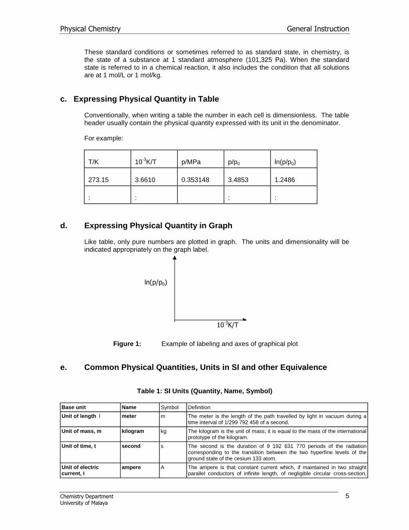
d. Expressing Physical Quantity in Graph Like table, only pure numbers are plotted in graph. The units and dimensionality will be indicated appropriately on the graph label.

e. Common Physical Quantities, Units in SI and othe r Equivalence

Table 1: SI Units (Quantity, Name, Symbol) Base unit Name Symbol Definition

Unit of length l meter m The meter is the length of the path travelled by light in vacuum during a time interval of 1/299 792 458 of a second.

Unit of mass, m kilogram kg The kilogram is the unit of mass; it is equal to the mass of the international prototype of the kilogram.

Unit of time, t second s The second is the duration of 9 192 631 770 periods of the radiation corresponding to the transition between the two hyperfine levels of the ground state of the cesium 133 atom.

Unit of electric current, I

ampere A The ampere is that constant current which, if maintained in two straight parallel conductors of infinite length, of negligible circular cross-section,

ln(p/p0)

10-3K/T

Figure 1: Example of labeling and axes of graphical plot



6

and placed 1 meter apart in vacuum, would produce between these conductors a force equal to 2 x 10-7 newton per meter of length.

Unit of thermodynamic temperature, T

kelvin K The kelvin, unit of thermodynamic temperature, is the fraction 1/273.16 of the thermodynamic temperature of the triple point of water.

Unit of amount of substance, N

mole mol 1. The mole is the amount of substance of a system which contains as many elementary entities as there are atoms in 0.012 kilogram of carbon 12; its symbol is "mol."

2. When the mole is used, the elementary entities must be specified and may be atoms, molecules, ions, electrons, other particles, or specified groups of such particles.

Unit of luminous intensity

candela cd The candela is the luminous intensity, in a given direction, of a source that emits monochromatic radiation of frequency 540 x 1012 hertz and that has a radiant intensity in that direction of 1/683 watt per steradian.

Table 2: SI UNITS and their equivalents Symbol

Physical Quantity

Unit Name

Definition of SI Units

not SI units

Equivalent forms of SI Units

l Length meter m m Angstrom 1010 m

m Mass kilogram kg kg micron 10-6 m

t Time second s s

I Electric current ampere A A

T Temperature Kelvin K K Degree Celsius T - 273.15

n Amount of substance mole mol mol

A Area m2 m2

V Volume m3 m3 Liter 10-3 m3

ρ Density kg m-3 kg m-3

v Frequency hertz Hz s-1 p.p.s.; p/s s-1

E Energy joule J kg m2 s-2 erg, calorie electron volt

10-7, 4.184 J 1.602 x 1019 J

q Quantity of heat J kg m2 s-2

F Force newton N kg m s-2 dyne 10-5 N

p Power watt W kg m2 s-3

p Pressure pascal Pa kg m-1 s-2 atmosphere torr/mm Hg

101 325 Pa 101 325/760 Pa

C Heat capacity JK-1 kg m2 s-2 K-1

S Entropy JK-1 kg m2 s-2 K-1 "entropy unit" kg m2 s-2 k-1

k Boltzman constant JK-1 kg m2 s-2 K-1

R Gas constant JK-1 mol-1 kg m2 s-2 K-1 mol-1 1 atm / deg mol 101.3 JK-1 mol-1

λ Thermal conductivity W m-1 K-1 kg ms-3 K-1

Q Electric charge Coulomb C A s e.s.u 3.336 x 10-10 c

∆V Electric potential different volt V kg m2 s-3 A-1 � Electrical resistance ohm kg m3 s-3 A-2

G Conductance siemens S kg-1 m-2 s3 A2

C Capacitance farad F kg m s A

L Inductance henry H kg m2 s-2 A-2

E Electric field strength V m-1 kg m s-3 A-1

κ Electrical conductivity S m-1 kg-1 m-3 s3 A2

P Dipole moment C m A s m debye 3.336 x 10-30 C m

α Polarizibility C m2 V-1 kg-1 s4 A2



7

ε Permittivity F m-1 kg-1 m-3 s4 A2

µ Permeability H m-1 kg m s-2 A-2

R Refractivity m3 m3

n Refractive index

I Magnetic flux weber Wb kg m2 s12 A-2

B Magnetic flux density tesla T kg s-2 s-2 A-1 gauss 10-4 T

H Magnet field strength A m-1 A m-1

µ ; m Magnetic moment J T-1 A m2

mB Bohr magneton J T-1 A m2

ν Wave number m-1 m-1

γ Surface tension Pa m kg s-2

η Viscosity (dynamic) Pa s kg m-1 s-1 poise 10-1 Pa s

I Moment inertia kg m2 kg m2

P Momentum N s kg m s-2

C Concentration mol m-3 mol m-3 M(mol l-1) 10-3 mol m-3

mB Molality mol kg-1 mol kg-1

M Molar mass (molecular mass)

kg mol-1 kg mol-1

f. Conventional Prefixes in Physical Quantities

Table 3: Common Prefixes

Factor Prefix Symbol Factor Prefix Symbol

10-1 deci d 101 deca da

10-2 centi c 102 hecto h

10-3 milli m 103 kilo k

10-6 micro m 106 mega M

10-9 nano n 109 giga G

10-12 pico p 1012 tera T

10-15 femto f

10-18 atto a

Table 4: Common Fundamental Constants

Symbol

Physical Constants

Values

c Velocity of light in vacuum 2.9979 x 108 m s-1

e Charge of proton 1.6023 x 10-19 C

k Boltzmann constant 1.3806 x 10-23 J K-1

h Planck constant 6.6262 x 10-34 J s

L or NA Avogadro number 6.022 x 1023 mol-1

F Faraday constant 9.6487 x 104 C mol-1

R Gas constant 8.314 J K-1 mol-1



8

4. Accuracy, Precision and Data Analysis a. Introduction

The general procedure in the usual experiment in elementary physical chemistry includes the following basic steps.

i. Measurements are made with certain instruments. Some of the instruments used are quite simple in nature, like a burette or a thermometer, for example; others are more complicated, like a potentiometer or a refractometer.

ii. The data from the measurements may be substituted with certain formulas or relationships in order to calculate other desired magnitudes.

iii. In the utilization and study of the various data, plotting procedures may be employed. In some cases a statistical study of the data is made.

If the various steps are to be followed in a proper scientific manner, attention must be given to the precision of the measurements and to the precision of the computed quantities. We must decide whether to make a single measurement of a given magnitude or a set of measurements in order to obtain the desired precision. This section of the manual deals, for the most part, with various definitions, equations, and concepts concerned with precision.

If a large number of measurements of a particular magnitude are made, statistical procedures are necessary to utilize the data properly. The manual includes, therefore, a discussion of the concepts, definitions, and equations used in statistical procedures. Because of the extreme importance of plotting procedures, discussion of this topic is given. This discussion, as well as the discussions of precision and statistical procedures, is on an elementary level. Those who wish to study these topics in greater detail may consult the bibliography for suitable references. The student should develop as soon as possible a precision-minded approach to the various experiments. The lack of proper attention to precision is one of the glaring weakness in most laboratory training.

b. Significant figures

We shall start our discussion of precision by defining the terms: certain figures, uncertain figures, and significant figures. These pertain to the process of making a measurement and recording the value obtained.

The instruments used in physical chemistry have what we shall refer to as least count. This is the smallest division of the instrument scale that can be read directly. The thermometer in Figure I has a least count of 1°, whereas a Beckmann thermometer, which is graduated in hundredths of degrees, has a least count of 0.01°. With most instruments, however,' you can estimate a reading to one digit beyond that which expresses the least count. In Figure 1, for instance, you can read a temperature of 25.2° and feel confident that you are within 0.2° of the prop er value.

In this value of 25.2° w e term the digits to the left of the decimal point certain figures and the digit to the right of the decimal point an uncertain figure. Although we have considerable confidence in the uncertain figure, we should express the extent of our certainty by writing the temperature as 25.2 ± 0.2°. If we record a volume measurement as 3 5.35 ± 0.05 ml, we



9

are confident that the actual value lies between 35.40 ml and 35.30 ml.

Of more importance than the terms certain and uncertain figures is the term significant figures. The significant figures in a measurement include both the certain and the uncertain figures. All of the figures in the readings 25.2° and 35.35 ml referred to above are significant figures.

The peculiarities of our number system require that zero be given special attention in considering significant figures. If the zero or zeros are immediately to the right of the decimal point, they serve merely to locate the decimal point. In 0.00013 g, the three zeros following the decimal point are not significant figures. However, in 0.130 g, the zero following the “3” is a significant figure. In 250 g, the zero may or may not be significant; it may serve merely to locate the decimal point. Any doubt, however, concerning this number would vanish if it were written:

2.50 x 102 g

Exercise1. Indicate the significant figures in each of the following:

0.0018 volt 1650 ml 12.5260 g 0.1800 volt 1.650 x 103 ml 1.65 dynes per cm 1.800 volt 1.65 x 10-3 ml 16.2 miles

c. Precision and Accuracy

The terms precision and accuracy are often used interchangeably, although they are actually quite different in meaning. Accuracy concerns the correctness of a measurement, whereas precision concerns the reproducibility of the measurement and the number of significant figures in its value.

To illustrate, let us measure the temperature of a constant-temperature bath with two thermometers, one with a least count, or ultimate subdivision, of 1° and one with a least count of 0.1°. With the first thermometer we read a temperature of 25.2 ± 0.2° and with the second a temperature of 25.18 ± 0.02°. The seco nd reading, with its four significant figures, is the more precise reading. In this sense we are using the word precise in connection with the number of significant figures which we can with confidence write down for the measured magnitude. The thermometer with the least count of 0.1° is the more precise instrument.

Now we may make a series of readings with a single thermometer. The readings may show little divergence among themselves, or they may differ rather widely. If the differences are small we may say that the method of measurement is one of high precision and that the procedure is a precise one.

Precise and accurate

Precise but not accurate Neither accurate nor precise

Figure 2 : The distribution of darts on dart board



10

In summary, precision concerns both the reproducibility of the magnitude and the number of figures we may with confidence express in the answer".

After we have made a number of readings of a given magnitude and sure that our values are precise in both senses of the word, we still do not know whether unknown or constant errors have entered into the determination. In measuring temperature, for example, there may be an error in the marking of the thermometer. Therefore, the recorded temperature, although very precise, may be entirely wrong. Accuracy deals with the difference between the measured value and the true value. Good precision does not insure high accuracy, but high accuracy is improbable without good precision. It is possible, on the other hand, to have high accuracy provided sufficient readings of fair precision are made and provided a proper statistical procedure is used.

It should be noted that, properly used, the term accuracy requires a modifying adjective. To say that a result is accurate means that it is exactly right. But only in a few cases do we know the exact value of the quantity being measured. Hence we should speak of a high order of accuracy or a low order of accuracy rather than stating merely that a result is accurate.

Let us now examine how we may express precision in a quantitative manner. One way to do this is to consider the extent of the uncertainty of the uncertain figure. If a temperature is recorded as 25.24 ± 0.02°, the value of 0.02° is a measure of the precision. We can speak of such a value as the least-count precision or, sometimes, the decimal precision. ! We note that it is expressed in the same units as the measured quantity. We may also express the preciseness of a measurement in terms of relative precision, which may be defined as the relative uncertainty of the measured magnitude. This is obtained by dividing the value of the magnitude into the least-count precision. The result may be expressed in parts per hundred (per cent) or in parts per thousand. The determination of relative precision is illustrated in Example 1.

Example 1 What are the least-count precisions and the relative precision in per cent of the two magnitudes? 25.26 ± 0.01 g and 125.26 ± 0.01 g? In both cases the least-count precision is 0.01 g.

The relative precisions are:

%04.010026.25

01.0 =×g

g %008.0100

26.125

01.0 =×g

g

Thus, we see that the least-count precision depends on the measuring instrument and the relative precision on the value of the magnitude being measured. You should note that the relative precision is dimensionless.

5. Error Estimation and the Use of Experimental Res ults

a. Introduction



11

A good experience is not necessarily one of high accuracy but one which will stand up to criticism which is reliable within the limits of accuracy claimed, and which achieves this result without fuss over irrelevant or unimportant details. A good experimenter has to strike the right balance between taking too much for granted and taking too little for granted. There is a danger at one extreme of neglecting important precautions, checks and corrections and at the other extreme of wasting time and energy over unnecessary refinement and repetitions. Between these extremes there is plenty of room for the exercise of individual judgment. The discussion of errors which fo1lows is intended for your guidance, but no rules can be laid down in which do away with the need for intelligence and common sense. The purpose of estimation errors is two fold. Error estimation is the basis of the design of experiments which achieve good results with economy of time and apparatus and it gives the limits within which the results are reliable when they have been obtained. The magnitude of possible errors should be kept in mind at all stages of the experiment and not just considered as an afterthought.

b. Systematic and Random Errors

A systematic error is one which occurs with the same sign in every reading, whereas a random error is one that is equally likely to be positive or negative. A systematic error is a constant error, whereas a random error is one that is, to some extent, unpredictable and only probabilistic statements can be made about it.

Suppose for example that the period of a pendulum is being measured by means of a stop-clock and the measurement is being repeated many times. The results obtained will vary, and if the measurement is subject to random errors only, some results will be too high and others too low. However, if the clock is running slow all the values will tend to be too low; this is a systematic error with random error superimposed. Another common cause of systematic errors is in unsuspected differences between the actual experimental arrangement and that assumed in the theoretical description of the experiment. If this difference is appreciated it can often be accounted for by a correction factor. Repetition of measurements serves two purposes with respect to random errors. First, it reveals their presence and leads to an estimate of their magnitude. Second, a goad estimate of a given quantity is the mean of a number of independent measurements; the greater the number, the closer the mean approaches the "true!' value. Neither of these remarks applies to a systematic error. Repeated measurements with the same apparatus do not reveal nor do they eliminate a systematic error. For this reason systematic errors are potentially more dangerous than random errors. If large random errors are present in an experiment, they will manifest themselves in a large value of the final estimated error, and the inaccuracy of the measurement is apparent. However, the concealed presence of a systematic error may lead to an apparently reliable result, given with a small estimated error, which is in fact seriously wrong. Unfortunately there is no general rule for finding and eliminating systematic errors. It is simply a case for thinking about the particular method of doing the experiment and drawing on past experience. It is sometimes possible to spot a systematic error by varying the experimental conditions (in the example above for instance, by using another clock). In general, it is wise to suspect ones apparatus and if necessary calibrate it against a standard of known accuracy. The remainder of these notes is concerned with the estimation of the magnitude of random errors. Some results from the theory of errors will be stated without proof. A good



12

elementary account of this theory can be found in “Errors of Observation and their Treatment” by J. Topping (Chapman and Hall 75p).

c. Error Distribution

Suppose that we take n successive measurements of some quantity and obtain the readings xl, x2, x3… xn: In the absence of random errors these values would be equal. However, in practice they are distributed around some mean value. Statistical theory attempts to describe this behavior by choosing a functional form for the distribution which matches the experimental observations as closely as possible. Several different distributions have been studied in this way but for our purposes we consider only the Normal or Gaussian Distribution. This has the advantage of being reasonably easy to handle mathematically but it must be remembered that it is often only a poor approximation to the real situation.

0

0.0005

0.001

0 2000 4000 6000 8000 10000

Curves which describe the normal distributions are shown above and these have a general form of

( )[ ]22 2xexp2

1y σµ−−

πσ= (1)

The area under the curve ∫∞

∞−

ydx is unity.

The interpretation of this curve is that the probability that an observation will lie between x and x + δ x is exp [- (x - � )2 / 2σ 2 ]δ x. The distribution is determined by 2 parameters � and σ . The parameter � is the mean of the distribution (since the curve is symmetric) and σ , called the standard deviation of the distribution, is a measure of its width or “spread". Thus a poorly determined set of readings with a broad spread (distribution 2) is described by a distribution with a large standard deviation σ 2 (for example) and conversely. The

Figure 3: Two normal distribution curves, defined typically by the means µ1 and µ2 and standard deviations σ1 and σ2. Although µ1 = µ 2= µ , but σ1 < σ2.

µ the mean for both the distributions

Distribution 1

Distribution 2



13

probability that an observation will lie within σ of the mean � is 68 %, while the probability that it will lie within a distance of 1.96 σ from � is 96 %. The quantity 1.96 σ is thus called the 96 % confidence limit.

d. The Best Estimate from the Mean and the Standard Deviation

We have n equally good successive measurements of a quantity xl, x2, x3,.... xn. Statistical theory says that, for a Gaussian distribution of errors, the best estimate of the quantity is given by the arithmetic mean.

i

x.......xxxx n321

∑

++++= (2)

and that the standard deviation σ s of a single observation can be estimated by

( ) 2

12

i

s 1n

xx

−−∑

=σ (3)

The quantity s is easily calculated using a desk calculator, making use of the relation

( )( )2

ii

i

2

i

2

ii n

xxxx

∑∑∑ −=− (4)

Suppose now that the set of n observations is repeated many times. The arithmetic mean of each set will vary from one set to another. That is to say, the arithmetic means will spread about their arithmetic mean and we may estimate σ for the arithmetic means just as we estimated the σ s for each single observation in equation (3). We expect σ m - the standard error for the arithmetic means - to be less than σ s, the standard error for a single observation. The larger the value of n, that is the more single readings that go into each arithmetic mean, the smaller would we expect σ m to be. In accordance with these common sense considerations, the theory of errors shows that

nsm

σ=σ (5)

The probability that the result x is within mσ of the true value is 68%; the probability that it

is within 2 mσ is adopted as a sensible estimate of the limits of error, i.e. that you quote

your results as

n/2xs

σ± . (6)



14

It is important to realize that, when many sets of n observations are made, not only does x vary from one set to another but so also does the calculated value of

sσ . In other

words, the value of s

σ obtained from one particular set is only an approximation to the

true value (i.e. the value that would be obtained from a set containing an infinite number of readings).

In an actual experiment, we only take one set of n readings and n may be as small as say 5. When we apply the above theory to estimate, mσ ; we must bear in mind that the value

obtained only an estimate and the smaller the value of n, the worse the estimate is likely to be. It follows that elaborate calculations based on the formulae of this section are quite pointless. Statistical theory gives order-of-magnitude estimates only. Therefore all calculations of estimated error should be rounded off to one significant figure, in general or two at most.

e. Rule for Rejecting Odd Data

When the values in a set of n observations are not same, there may be odd data which deviate too far from the mean value. We may be able to determine these odd data if we analyze in detail these records. For example, in the acid-base titration, a numbers of burette readings of acid solution obtained are shown as follows:

Table 5: Burettes reading in cm3

V1 V2 V3 V4 V5 V6 V7

26.86 25.28 25.30 24.60 25.30 25.32 25.34

If the reading of V1 = 28.68 cm3 is a rough reading which is done in the beginning of titration, we can just neglect it. However, the value of V4 looks odd; but we are uncertain if it can be neglected totally since we could not find any mistake on the titration method. On the decision whether to reject or accept the odd data, we often use the Chauvenet criterion, which evaluate the difference, d, (d=Vi - <V>), between one value Vi and its average. If |d| is more than |Q x σs| (Q times of the single observation standard deviation, σs), then Vi is rejected. This criterion can be used for one set of n observations when the n value is more than 4 (including the doubtful observation). The Q value is the boundary of rejectability and it depends on the number of data.

Table 6: Q for a number of observations

N (observation) Q 5 1.65 10 1.96 20 2.24 50 2.58

Thus in the above example, the average volume of the acid solution for all six reading (not including V1) is 25.19 cm3 and the standard deviation σs = 0.29. The difference between 25.19 and V4 are 0.59. By using the Chauvenet criterion we found that the difference (V4 -<V>) is more than 1.65 x σs (=0.48), therefore the V4 reading must be rejected.



15

222

+

≅

BAxbax σσσ

The true average burette volume <V> and its standard deviation σs is recalculated base only on five readings and we found that <V>= 25.31 cm3, σs = 0.02 cm3.

f. Combination of Errors in Several Quantities

The result of an experiment usually depends on a number of measured quantities, each of which is subject to some error. We want to know how to combine these errors to obtain the errors in the final result.

Let the final quantity be X and the directly measured quantities A, D, C, ... . Let the errors ( ei. . m ) in A, B, C... be σ a , σ b , σ c , ... and the resulting error in X be σ x. The relation between the errors for x various functional forms of X are given below:

1. X = A + B + C….

X = A – B ± C….

2. X = AB

X = A/B

3. X = An

Table 7: Errors for different functions

These relationships hold provided A, B, C… are statistically independent. Most of the commonly occurring functions can be built up from these forms. When a more complicated function of a measured quantity enters into the formula, the following method may be useful. Suppose m is the best experimental estimate and m' the greatest or least value of the same quantity which would not be obviously incorrect experimentally. If the required quantity is X = f(m), x' = f(m') should also be evaluated; then σ x is [X - X']. This method is always applicable and may be easier and more informative than other methods which are mathematically more elegant.

We recall that the estimates that are made of component errors are only approximate and so in turn is the error ' in the final quantity X. A value of σ x good to about 20% is

adequate. We see from the table above x that for case 1, if σ b is less than about 3

1 σ a its

contribution to σ x may be safely be neglected. The same is true in case 2 if B

bσ is less

than about Aaσ

3

1. It is therefore very important that energy is devoted to reducing the

error in those quantities whose errors contribute most to the final error. g. Graphical Treatment and Error Estimation

......+σ+σ+σ=σcbax

An

xax σσ

≅



16

A graph is often a convenient way of presenting a large number of data points for assessment. Experimental scatter is displayed, significant trends can be assessed and a theoretical model tested by a single graph.

Estimated range of error or standard deviations should be inserted. In the first place, these Ii error bars1i are required to decide on the scale, which should not depend on the size of the page. If the estimated range of error occupies most of the area of the graph, a wider range of observations should be included. At the other extreme, if the estimated error is comparable with the thickness of a pencil line, the graph is not the most accurate way of handling the observations.

Any line which fits all the experimental points within their estimated error ranges is an agreement with experiment. It is easy to test straight line relations in. this way; other curves are more difficult but not impossible. Small residual misfits may well be due to underestimation of the limits of error of individual readings. If any points are badly out from the single curve, they should be cheeked at once for real mistakes. If none can be found the experimenter must decide between 3 possibilities:

(a) the estimate of the limits of error was too optimistic (b) a mistake remains, in spite of search and the point must be disregarded (c) the theory being tested is incorrect

Quantitative results are much more easily obtained from a straight line graph than from any other curve. It is therefore wise to manipulate the theoretical formulae where possible so they are in linear form.

The “best straight line” can then be drawn through the data points taking due account of the error bars and the slope and intercept measured. When plotting a graph, the range of measurements and hence the scale should be chosen so that full use is made of the paper, i.e. the line should run diagonally across the sheet.

Again, the gradient of the line should be estimated from the whole of the graph, not from a small triangle constructed in the top left--hand corner. Rough estimates of the error in the slope or intercept can be made by seeing how far the line can be tilted or displaced without going seriously outside the estimated error ranges of the separate points.

However, there are proper statistical methods for determining the best straight lines and the error in its slope and intercept, and these are discussed in the next section.

Figure 4: 3 plots for spring extension, x versus mass, m. (a) Plot without error bar. (b) The same data plotted with error bar if the error of m is expected to be very small, the error is only in x. (c) Graph shows one set of inconsistent data of direct proportional between x and m.



17

For example, Figure 4 shows the graph of m versus length x for spring. To estimate the error for each dependent variable which is x, we draw vertical error bars. The best line will go through all or close to every point (because the relationship between m and x, will intercept the origin). The spring constant can be obtained from the graph slope 4(b), if we draw two more lines L1 as the most vertical line and L2 as the most horizontal line. Both lines will have k1 and k2 slope respectively (where k1>k>k2)

The error for k, dk can be obtained from : δ k=(k1 – k2) / 2

Remember that both L1 and L2 lines must go through or close to every error bar.

In figure 4(c), if Hooke’s Law for spring is true, therefore the data obtained is just not consistent and all these show that these experiments have problems that need to be solved.

h. Linear Least Square Method

Suppose yl y2 ... yn are the values of a measured quantity y (or combination of measured quantities) corresponding to values x1... xn of another quantity x.

Let us assume for simplicity that there are experimental errors in the values of yi but not in the values of xi. Conditions closely approaching these, where the errors in one of the variables may be neglected, often occur in practice. We assume too that there exists a linear relationship between x and y, namely baxy +=

On substituting x = xi, the value of y will not in general equal yi; There will be an error or residual of amount

iii ybaxr −+= (7)

A typical plot showing the residuals is

Figure 5 : A graph shows the residue amount



18

According to the principle of least squares, the line which best fits the observed data is defined by values of a and b for which the sum of the squares of the residuals is least, that is

2

∑=i

irV is minimized.

Now ( )2

∑ −+=i

ii ybaxV (8)

The minimum with respect to a and b is given by

( )∑ −+==∂∂

iiii ybaxx0a

V (9)

( )ii

i ybaxbV −+==∂∂ ∑0 (10)

i.e. 02 =−

+

∑∑∑ i

ii

ii

Ii yxbxax (11)

0=−+

∑∑

ii

ii ynbax (12)

Hence 2

2

−

−

=

∑∑

∑∑∑

ii

ii

ii

iii

ii

xxn

yxyxn

a (13)

22

2

∑−∑

∑∑−∑∑

=

i ixi ixn

i ixi iyix

i iyi ix

b (14)

The error of both a and b are given as follows;

2/122 ]})()(/[{ iiya xxnn ∑−∑= σδ (15)

2/1222 ]})()(/[){( iiiyb xxnx ∑−∑∑= σδ (16)

where, 2/12)]2/()[( −−−∑= nbaxy iiyσ (17)



19

Example: Least Square Method

x y x2 xy

1.0 5.4 1.0 5.4

3.0 10.5 9.0 31.5

5.0 15.3 25.0 76.5

8.0 23.2 64.0 185.6

10.0 28.1 100.0 281.0

15.0 40.4 225.0 606.0

20.0 52.8 400.0 1056.0

Σx = 62.0

Σy = 175.7

Σx2 = 824.0

Σxy = 2242.0

By using equation (13) and (14)

a = [(62.0) (175.7) - 7(2242.0)] / [(62.0)2 - 7(824.0)] = 2.495

b = [(2242.0) (62.0) - (175.7) (824.0)] / [(62.0)2 - 7(824.0)] = 3.00 therefore, y = 2.495 x + 3.00 To get slope deviation and intercept we use equations 15, 16 and 17.

(yi - axi - b)

(yi - axi - b) 2

0.095

0.0090

0.015

0.0002

0.175

0.0306

0.240

0.0576

0.150

0.0225

0.025

0.0006

0.100

0.0100

Σ( yi - axi - b)2 = 0.1305

σ2 = {Σ|yi - axi - b| 2 / (n - 2)}

δa = 0.1615 {7 / [7(824.0) - (62.02)2 ]} 1/2 = 0.0097

δb = 0.1615 {824.0 / [7(824.0) - (62.02)2 ]} 1/2 = 0.106

Hence,

a = 2.495 + 0.010 b = 3.00 + 0.11



20

6. General equipment and Tools

a. Barometer

Brometer is an instrument to measure the atmospheric pressure. Many thermodynamic quantities vary in their values according to the atmospheric pressure and the ambient temperature. Therefore, it is important to record the room temperature and pressure when measuring any physical quantities. Our physical chemistry laboratory is equipped with the Fortin barometer (model J297 and R589).

The Fortin barometer is named after its inventor, Nicolas Fortin. It features a cistern partly made of glass, in which one can observe the lower level of the mercury and determine the zero point of the barometric scale. Before reading the height of the mercury column in the barometric tube, it is necessary to adjust the mercury level in the cistern so that it coincides with the tip of an ivory reference screw. This adjustment is performed by modifying the position of the cistern's leather bottom by means of a screw. The tube, which is lost, was enclosed in a brass tube with small windows to observe the mercury level. The tube is fitted with a vernier for readings and carries three engraved scales. There is also a mercury thermometer with a centigrade scale.

To read the pressure, read the rough value from the main scale (eg. 757 in the above figure). Then read from the vernier scale a line that is aligned with the main scale. The vernier scale is correct to two decimal places (±0.05 mm Hg). Thus the reading of the atmospheric pressure is 757.65 + 0.05 mm Hg.

Main Scale Vernier Scale

Porous Material

Fiducial point

Screw

Fixed scale

Vernier scale

Accurate reading 757.65 mmHg

Rough reading 757 mmHg

Zero line

Mercury meniscus

Figure 6: Fortin Barometer to measure the atmospheric pressure



21

Temperature correction of the pressure reading from the barometer must be made if the reading is to be corrected to 273.15 K. The following table 13 gives the correction factor.

Table 13:

Temperature correction factors (in mm Hg), pressure reading at 273.15K.

b. Bibliography and Information Databases

When working in physical chemistry laboratory, often you need to refer to standard numerical values of physical measurements. You may find these tabulated quantities in books of physical constants such as the CRC Handbook of Chemistry and Physics 1999-2000:80thed) by David R. Lide (Editor) (which is provided in the laboratory) or one which you are recommended to purchase for example SI Chemical Data, Gordon Aylward and Tristan Finlay. Here we list some on-line data bases which may be useful to you. i. SciFinder Scholar

SciFinder Scholar provides online access to several databases, including Chemical Abstracts, Registry, CASREACT, CHEMLIST, CHEMCAT, and MEDLINE

ii. Beilstein BEILSTEIN is a major structure and factual database in organic chemistry

iii. Sciencedirect An information source for scientific, technical, and medical research www.sciencedirect .com

iv. SPECINFO The SpecInfo database system at Daresbury is a database management system from Chemical Concepts designed to store, retrieve, and manipulate NMR, IR, and mass spectra

p/mm Hg

T/K

750

760

770

298

3.05

3.09

3.13

299

3.17

3.21

3.26

300

3.29

3.34

3.38

301

3.41

3.46

3.51

302

3.54

3.58

3.63

303

3.66

3.71

3.75



22

v. ChemFinder

Collects, organizes, indexes and displays information on chemical substances, including physical property data and 2D chemical structures, and links to sites with more information. The database is searchable by chemical name, formula, molecular weight, and CAS Registry Number. Chemical structures may be viewed in ChemDraw or Chem3D, http://chemfinder.cambridgesoft.com/

vi. TORVS Software for reaction prediction, synthesis design, classification of organic reactions, chemical information, calculation of 3D coordinates for Chemical Structures. www2.chemie.uni-erlangen.de/services/

vii. VRML Resources for Chemistry www.sienahts.edu/~che/vrmlchem.html

viii. SciSearch® A Cited Reference Science Database is an international, multidisciplinary index to the literature of science, technology, biomedicine, and related disciplines

c. Computational Chemistry Resources

In addition, we also list here some computational chemistry resources which may be of some use to you if not immediately but for the future. i. MestReC

NMR processing software www.mestrec .com/

ii. HyperChem HyperChem is an easy-to-use molecular modeling program that allows the analysis and visualization of simple or complex molecules. It is equipped with several computational methods for calculating molecular geometry optimization, total energy, and bond angles and distances. It employs an intuitive point-and-click interface that allows for the easy assembly and calculation of molecule structures.

iii. Amber Amber is a package of programs for molecular dynamics simulations of proteins and nucleic acids.

iv. ChemDraw ChemDraw is the industry leader of chemical drawing programs. ChemDraw includes stereochemistry recognition and display, multi- page documents, ChemNMR with spectral display, and Name=Struct for instant structure generation. AutoNom creates IUPAC names from structures. ChemDraw for Excel brings chemistry to Excel. The Online menu links to ChemACX.Com for easy chemical sourcing and ordering. The ChemDraw Plugin adds chemical intelligence to your browser for querying databases and displaying data from web sites.

v. ISIS/Draw ISIS/Draw is a chemical drawing program somewhat similar to ChemDraw. It works in a slightly different way, so it will take a while to get used to using it.

vi. ChemWindow



23

Program for drawing 2-D chemical structures, laboratory apparatus, and chemical engineering flowcharts.

vii. WinNMR WINNMR is a tool for professional processing, analysis, annotation and plotting of NMR spectra.

viii. ArgusLab ArgusLab is a molecular modeling program that runs on Windows 98, NT, and 2000. ArgusLab consists of a user interface that supports OpenGL graphics display of molecule structures and runs quantum mechanical calculations using the Argus compute server. The Argus compute server is constructed using the Microsoft Component Object Model (COM). http://www.planaria-software.com/

7. Scientific Writing

A portion of scientific activity is to deliberate scientific findings to other people. Apart from verbal deliberation, writing is also commonly adopted. These may be in the form of a simple report, a long publication or even a thesis. Thus, in order to determine which format to adopt for the report, one must know the audience who will read the report. An extensive discussion on how to write a scientific and technical report may be found in many publications (eg.http://www.writing.eng.vt.edu/workbooks/laboratory.html).

a. Log Book

A scientist keeps all information on his/her experiment neatly and orderly. Thus, as part of your training to become a good scientist, you MUST have a log book or sometime it is called a jotter book. Everything you do and measure in the day must be reported in the jotter book. DO NOT use loose papers to record your results. You may lose them. Moreover this log book or jotter book must be numbered and dated accordingly. It is also useful to have a carbonized jotter book which allows you to hand a carbonized copy of the result to the lab supervisor which in this case, the lecturer-in-charge. The log book should be readable to you after many years and certainly readable to other people.

b. Formal Report Apart from keeping the laboratory log book, you are required to write a short formal report on every experiment assigned to you. Some lecturer may wish to assign you to write an extended report for one of these experiments. Please discuss with your lecture-in-charge for a detail format. Two types of report styles which we recommend are: a short scientific report and an extended scientific report. a. A Short Formal Report will have the following format:

i. Title Page ii. Results and Discussion iii. Conclusion iv. References

b. An Extended Formal Report will have the following format

i. Title Page ii. Background and Theory



24

iii. Procedure iv. Results and Discussion v. Conclusion vi. Future Work vii. Appendices viii. References

Briefly, as commonly practiced by our physical chemistry students in this department,

we shall discuss here the content items in both the short formal reports: Title Page: It contains the title of the experiment, the date when the experiment was conducted, your name and your partner’s name (if any), your group and location of the laboratory. Background and Theory In short formal report, it is unimportant to write the “Background and Theory” unless you are using different theory than that suggested in the experimental manual. You may simply refer to the manual. Procedure Likewise, in short formal report, it is unimportant to write the “Procedure” since this is already clearly stated in the manual. If however, a different procedure is adopted for some reason (and this may happen), you must report this clearly. Results and Discussion:

All raw and processed results must be recorded neatly and clearly. Repeated values may be tabulated with clear headers. If there is more than one table, please give a clear and legible title to each one of them.

Discussion section aims to analyze the results you obtain. This is done by describing

them, explaining the results with respect to the theoretical expectation either by proving the theory or otherwise. When results are in agreement with the theory, (you may feel happy) the discussion may be written in support of the theory which may now be used to predict other possible conditions. However, if result differ from the expected, the discussion may be more interesting. Here is the case when the theory may be weak or wrong or the experimental result is wrong. Discussion may be centered in scrutiny of the theory and all its assumptions or on the other hand, on possible sources of errors in the experimental procedure.

Conclusion

This summarizes the experimental findings and relates them to the objectives of the experiment.

References These days, no scientist works in isolation. Thus, as a good scientific practice, the

reference section must be included to make students aware the experiment they conducted is related to many other previous works which have been reported in the literature.



25

c. Example of Short Formal Report

Title Page

Experiment No.3 Title : Kinetics Chemistry: The hydrolysis rate of methyl

acetate at 30.5°C Date of expt: 11 July 2007 Name: Sarah Matrix No.: SES070001 Lab partner: Amy Matrix No.: SES070002 Group: 1230A Laboratory: Physical chemistry 1st year Lecturer: Prof. Ramli Ahmad

Objective: To determine the hydrolysis rate constant, k of methyl acetate catalyzed by HCl 0.5M and to calculate the half time, t½ of the reaction at 30.5°C.

Result:

Table 1: Temperature of water bath

Time, t (minute) Temp.,(°C)

0 30.50

15 30.50

30 30.50

45 30.50

60 30.50

75 30.50

90 30.50

Average 30.50

Plagiarism Warning!

Some of these experiments are carried out in groups of usually a pair of students. Therefore expectedly, each member of a group followed an identical procedure in the laboratory and has the same set of raw data. Members of a group are allowed to discuss the analysis of data with one another. However, preparation of the report including data analysis, interpretation and discussion must be prepared by the individual student submitting the report. The Department does not tolerate plagiarized report!



26

log 10(V∞-Vt)vs time

y = -0.00227x + 1.40229

R2 = 0.99968

1.2

1.25

1.3

1.35

1.4

1.45

0 20 40 60 80 100

time,t / minute

log

10(V∞

-Vt)

Table 2: Values of t, Vt (V ∞ -Vt) and log10(V ∞ -Vt)

Time, t Reading of buret, V

(ml) Vol. of NaOH, Vt (V ∞ -Vt), log 10(V ∞ -Vt)

(minute) initial final (ml) (ml)

0.00 0.65 21.90 21.25 25.35 1.404

10.00 21.90 44.60 22.70 23.90 1.378

20.00 2.40 26.35 23.95 22.65 1.355

30.03 1.80 26.80 25.00 21.60 1.334

46.28 2.85 29.60 26.75 19.85 1.298

60.05 0.20 28.35 28.15 18.45 1.266

80.06 3.50 33.50 30.00 16.60 1.220 ∞ 1 0.05 46.35 ∞ 2 0.50 46.85 46.60

Graph 1: Log (V ∞ - Vt) vs. time, t

Discussion : Methyl acetate hydrolyzes to form acetic acid and methanol, according to the following reaction: (1) The reaction is extremely slow in pure water, but is catalyzed by both hydronium and hydroxide ions. In this experiment the kinetics of the reaction catalyzed by HCl 0.5M was studied.

CH3

O

OM e

OH2 CH

3

O

OH

CH3OH+ +



27

Hydrolysis reactions of this type are reversible; the back reaction is called esterification. For any equilibrium the overall rate is the difference in rates of the forward and reverse reactions: Rate = Rate forward – rate reverse (2) If, however, the reaction is not allowed to proceed very far to the right, the concentrations of products will be very small and the reverse rate term can be neglected. Thus, during the early stages of the reaction the rate law is written: Rate= -dc/ dt = kc (3) From graph 1, the slop, m is refer to the rate of hydrolysis Slope, m =

�log (V ∞ - Vt)/

�t

Rate of hydrolysis = 2.1 x 10-3 min-1 The reaction is first-order with respect to both methyl acetate and water of order 1 (determined in experiment) with respect to H3O

+.To calculate the hydrolysis rate constant, k of the hydrolysis of methyl ester, For the first order reaction: Slope, m = -k/2.303, from the graph 1, m = (-0.00227 ± 0.00002) min-1 k= 0.00522781 min-1 To calculate the error of the hydrolysis rate constant,

�k: �

k =�

m / m x k �k =0.00002 / 0.00227 x 5.30 x 10-3 min-1 �k = 4.6696 x10-5 min-1

Therefore, the hydrolysis rate constant, k of the hydrolysis of methyl ester, k = (5.228 ± 0.005) x10 -2 min -1 The rate also can be written as, Rate = -d [CH3COOCH3]/dt = k [CH3COOCH3] [H2O] [H3O

+] or Rate = dx/dt = k (a-x) (4) Where, a = the volume of NaOH was used until the reaction completed (The initial concentration of methyl acetate)(46.60 ml) x = the volume of NaOH was used for the given time

(The amount of methyl acetate was react after t time) The integrated equation (4) gives, Log [a/ (a - x)] = kt/2.303 (5) Log (a - x) = -kt/ 2.303 + log a (6) For half life, t½ of the reaction, the amount of methyl acetate was reacting after t time is (x/2).



28

Log (a – x/2) = -kt½ / 2.303 + log a -kt½/2.303 = log (a/2) – log a - (5.228 x 10-2 minute-1) t½/2.303 = log [(a/2) / log a] - (5.228 x 10-2 minute-1) t½/2.303 = log [(46.60/2) / log 46.60] - (5.228 x 10-2 minute-1) t½/2.303 = 1.147 - (5.228 x 10-2 minute-1) t½/2.303 = (1.147 x 2.303)/ (5.228 x 10-2 min-1) - (5.228 x 10-2 minute-1 /2.303 t½= (1.147 x 2.303)/ (5.228 x 10-2 min-1) - (5.228 x 10-2 minute-1 /2.303 t½= 505.377 min

The error of the half time,

�t½= (

�k / k) x t½

The error of the half time, �

t½= (0.005 / 5.228) x 505.377 The error of the half time,

�t½= 0.48 min

Therefore the half time of thereaction hydrolysis of methyl acetate is, t½= (505.4 ± 0.5 )min

Conclusion: From experiment the hydrolysis rate constant, k of methyl acetate catalyzed by HCl 0.5M is (5.228 ± 0.005) x10-2 min-1and the half life, t½ of the reaction is (505.4 ± 0.5 )min at 30.5°C. References

1. http://itl.chem.ufl.edu/4411L_f00/kin/kin.html 2. B.H. Mahan, “University Chemistry”, Addison-Wesley, (1972)

Chapter 9. 3. A. Findlay, “Practical Physical Chemistry”, Longmans, (1955) pp

297-300. 4. Williams, K. R. Laboratory Manual for Introductory Analytical

Chemistry; fall, 1995 (or later edition); pp 44-47.

general laboratory instructionrh23-06 · return the signed proclamation form to the departmental...

Documents