gene-hull catamaran 3.0 user guide english version 3

As for 2021 02 26 1/39

Gene-Hull Catamaran 3.0_User Guide_English version

This Catamaran version 3.0 of the application includes :– the Hull generation using a new version of the « E generalised » shaped sections (E for

Elliptical), well adapted for multihull. Leading to a simplification as the previous « UE » combination is no longer necessary.

– An 3D isometric view of the hull is now also output,– The stability study can be done with a loading, the output data are detailed for each hull

(leeward and windward ones) as well as for the catamaran as a whole, and can be used to fulfill the input data necessary for SA-VPP Catamaran (also offered separately).

– A specific sheet « Offsets x,y,z » is proposed , where all the geometrical output data are gathered and can be copy/paste for a transfer towards software tools oriented for engineering studies or 3D renderings.

Gene-Hull Catamaran makes possible the generation of hulls with their 2D views and theirhydrostatic characteristics as output, daggerboard and rudder included. It is based on aspreadsheet application (Open Office Calc 4.0.1) involving fit for purpose formulations of thepolynomial type, able to generate the hull fairing lines. It needs a relatively small number of datato enter : basic geometrical data, parameters used in the formulations. This User Guide gives alldefinition and information on the role and influence of each data, with illustrations. Moreover, theUser has the input data of a reference hull allowing him to start his own project step by step, and a« Hulls storage » sheet where other examples of inputs are archived and can be copy/paste.

For each new data introduced, all the computations and the drawings are updated automatically.Proposed parameters allow an infinity of combinations, so as many possible variants of a hull.Drawings and hydrostatic data, including ratios usually considered by naval architects, makepossible to judge the hull and to converge towards the desired one. In section 5. of the results, thecomputation of the heeled catamaran is also proposed, in hydrostatic condition, at isodisplacement and with control of the longitudinal center of buoyancy thanks to iteration on heightand trim parameters. It provides the righting moment, and 2D drawings (sections and floatationwaterline) which can help assess the relevance of the hull with heel.

Produced data allow either to continue the project with a 3D modeller (for that option, allnecessary data are provided in section 5.) or, for amateurs in particular, to draw at scale one anysections and frames needed for a building (data are provided in section 7.).

In the present state of this development, some limitations exist which could be overtaken withinfurther versions. Main is :

– necessarly inverted (or quasi vertical) rear transom (but hull with classic transom can begenerated, it is just that the transom itself is not drawn)

– no inverted bow possible

After an apprenticeship that should be light thanks to this User Guide and the hull of referencegiven to initiate a new project, it is easy and even fun to create a great number of hulls within justfew clicks, up to test unusual values of parameters to find out new style or shape of hulls :combinations are infinites and sometimes unpredictables (it is also a way to test the limits of this

As for 2021 02 26 2/39

software). Of course at the end, the final choice is up to the User, taking into account hisexperience as naval architect.

It is a free and open source speadsheet application, on a support itself free and widespread (OpenOffice Calc 4.0.1) : if any problem are faced to open and use an ods file, you can download OpenOffice or Libre office according to : http://www.openthefile.net/extension/ods

In case of, you can contact me with your remarks and improvement requests.

Jean-François Masset - February 2021 contact : [email protected]

http://www.openthefile.net/extension/ods

mailto:[email protected]

As for 2021 02 26 3/39

Summary presentation

The application includes 5 sheets :– Gene-Hull – Hulls storage – Sailplan– Mass spreadsheet– Offsets x, y, z

Gene-Hull : includes an User space (input & outputs) followed by an Administrator space (from line356) where the computations are carried out. The User space includes 5 successive sections :

Gene-Hull input : 1. Data to enter

Gene-Hull output :2. Data sum-up and results of hydrostatic and surfaces calculations 3. The 3 views 2D4. Curves of control

Gene-Hull complementary input and output5. Stability and righting moment with a loading

Hulls storage : is the storage space for hulls input data

Sailplan input and output :includes an User space (input and output, 2D view of the sailplan)followed by an Administrator space where the computations are carried out

Mass spreadsheet input and output : includes an User space (input and outputs)

Offsets x,y,z : where all the geometrical output data are gathered and can be copy/paste for atransfer towards software tools oriented for engineering studies or 3D renderings

To open and use the application :It is a speadsheet application in .ods format, developed with Open Office Calc 4.0.1, which can beused with Open Office or Libre Office : if any problem are faced to open and use an ods file, youcan download Open Office or Libre office according to : http://www.openthefile.net/extension/ods

http://www.openthefile.net/extension/ods

As for 2021 02 26 4/39

The coordinates x,y,z used for the « one hull » views include : – Origin 0,0,0 at the cross of the designed waterline surface (« H0 » level) and the

perpendicular at the rear point of the waterline (station C0). The perpendicular at the frontpoint of the waterline is station C10.

– x = longitudinal axis (positive towards front), – y = transversal axis,– z = vertical axis (positive towards up), Showed unities on the views are cm

Automatic scales are proposed for the views, with a main grid with a fixed pitch. Nevertheless, it issuggested for the User, as long as the main dimensions of the new project are fixed, to put theviews at a right scale and to fix it. For the catamaran views with its 2 hulls, the longitudinal axis isthe catamaran axis of symmetry.

-200 -100 0 100 200 300 400 500 600 700 800 900 1000 1100 1200 1300 1400 1500 1600 1700

-400

-300

-200

-100

0

100

200

-150 -100 -50 0 50 100 150

-350

-300

-250

-200

-150

-100

-50

0

50

100

150

-150 -100 -50 0 50 100 150

-350

-300

-250

-200

-150

-100

-50

0

50

100

150

-200 -100 0 100 200 300 400 500 600 700 800 900 1000 1100 1200 1300 1400 1500 1600 1700

-200,00

-100,00

0,00

100,00

200,00

As for 2021 02 26 5/39

Gene-Hull sheet / Input

1. Data to enter for the hull bodyData to enter are in lines B12 to B54. Data are in metric units, with an automatic conversion inImperial units in column C (in italic blue in the file).

1.1 Hull data metric >> feet

Lwl (m) 15,00 49,21Beam between hulls axis

Bhu (m) 6,10 20,01

Tc (m) 0,77 2,53X Tc (%Lwl) 45,0

Xbow (m) 15,25 50,03Zbow (m) 1,15 3,77

Cet 90Polynomials of the keel line, front part and rear part :

Pui q av 2,20Pui q ar 2,20

X tab ar (m) -0,75 -2,46Z tab ar (m) 0,170 0,56

Bg (m) 0,80 2,62X Bg (% Lwl) 56,5

Alfa (°) 3,90Pui liv y 2,00

Cor Pui liv 0,020Pui Cor Pui 1,00X liv ar (m) -0,20 -0,66

Scow 0,10

Type 11,2 Zhc av (m) 0,24 0,79

2 Zhc m (m) 0,65 2,131,2 Zhc ar (m) 0,5 1,64

Pui hc z 1

Z liv m (m) 1,2 3,94Z liv ar (m) 1,10 3,61

Deck / central line rear end Z p m (m) 1,25 4,10X p ar (m) -0,30 -0,98Z p ar (m) 1,15 3,77

Pui E1 av 1,20 Pui E2 av 2,00Pui E1 mid 0,79 Pui E2 mid 3,04

Pui E1 ar 0,65 Pui E2 ar 2,53

Lenght of waterline :

Maximum draft of the hull body :

Hull bow :

Shape coefficient of the bow :

Rear end of the transom :

Sheer line, in horizontal projection xy :

Option Hard Chine line, in vertical projection xz :

Sheer line, in vertical projection xz :

Sections « E » shape (E like Elliptic) sections

As for 2021 02 26 6/39

Lenght of waterline

Lwl (m) : lenght of waterline at H0 (cell B12)

Rear perpendicular crosses H0 plan at the coordinates origin (0, 0, 0). Front perpendicular crosses H0 at (Lwl, 0,0) point.

Beam between hulls axis

Bhu (m) : transversal distance between the 2 hulls axis (cell B14)

Hull body draft

Tc (m) : maximum draft of the hull body (cell B16)

X Tc (%Lwl) : longitudinal position of the maximum draft (in % of Lwl) (cell B17)

Example with X Tc : 40 %Lwl



Hull bow end

Xbow (m) : should be > Lwl (inverted bow is not possible) (cell B19)

-200 -100 0 100 200 300 400 500 600 700 800 900 1000 1100 1200 1300 1400 1500 1600 1700

-100

0

100

200

-200 -100 0 100 200 300 400 500 600 700 800 900 1000 1100 1200 1300 1400 1500 1600 1700

-100

0

100

200

-200 -100 0 100 200 300 400 500 600 700 800 900 1000 1100 1200 1300 1400 1500 1600 1700

-100

0

100

200

As for 2021 02 26 7/39

Zbow (m) : it is the front freeboard (cell B20)

Bow coefficient

For the bow shape, in addition to Xbow and Zbow acting on the front overhang, one parameter isinfluent and in interaction : Cet

Cet : adimensional coefficient > 0, from 0,1 to 100 typically. (cell B 22)This coefficient is involved in the polynomial formulation of the front part of the keel line andmostly influence the bow shape. Examples with same Xbow, Zbow :

Cet = 1 :

Cet =20 :

Cet 40 :

Cet 80 :

² Cet 160 :

-200 -100 0 100 200 300 400 500 600 700 800 900 1000 1100 1200 1300 1400 1500 1600 1700

-100

0

100

200

-200 -100 0 100 200 300 400 500 600 700 800 900 1000 1100 1200 1300 1400 1500 1600 1700

-100

0

100

200

-200 -100 0 100 200 300 400 500 600 700 800 900 1000 1100 1200 1300 1400 1500 1600 1700

-100

0

100

200

-200 -100 0 100 200 300 400 500 600 700 800 900 1000 1100 1200 1300 1400 1500 1600 1700

-100

0

100

200

-200 -100 0 100 200 300 400 500 600 700 800 900 1000 1100 1200 1300 1400 1500 1600 1700

-100

0

100

200

Xbow , Zbow

As for 2021 02 26 8/39

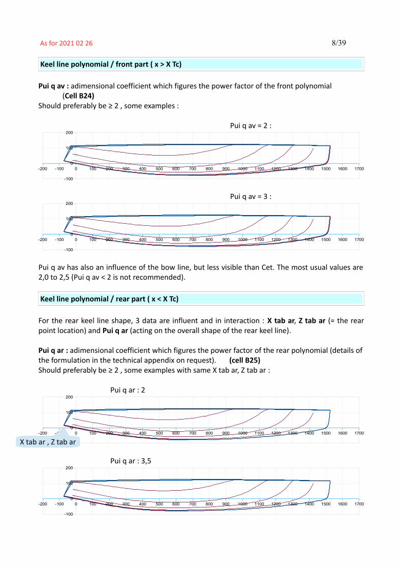
Keel line polynomial / front part ( x > X Tc)

Pui q av : adimensional coefficient which figures the power factor of the front polynomial (Cell B24)

Should preferably be ≥ 2 , some examples :

Pui q av = 2 :

Pui q av = 3 :

Pui q av has also an influence of the bow line, but less visible than Cet. The most usual values are2,0 to 2,5 (Pui q av < 2 is not recommended).

Keel line polynomial / rear part ( x < X Tc)

For the rear keel line shape, 3 data are influent and in interaction : X tab ar, Z tab ar (= the rearpoint location) and Pui q ar (acting on the overall shape of the rear keel line).

Pui q ar : adimensional coefficient which figures the power factor of the rear polynomial (details ofthe formulation in the technical appendix on request). (cell B25)Should preferably be ≥ 2 , some examples with same X tab ar, Z tab ar :

Pui q ar : 2

Pui q ar : 3,5

-200 -100 0 100 200 300 400 500 600 700 800 900 1000 1100 1200 1300 1400 1500 1600 1700

-100

0

100

200

-200 -100 0 100 200 300 400 500 600 700 800 900 1000 1100 1200 1300 1400 1500 1600 1700

-100

0

100

200

-200 -100 0 100 200 300 400 500 600 700 800 900 1000 1100 1200 1300 1400 1500 1600 1700

-100

0

100

200

-200 -100 0 100 200 300 400 500 600 700 800 900 1000 1100 1200 1300 1400 1500 1600 1700

-100

0

100

200

X tab ar , Z tab ar

As for 2021 02 26 9/39

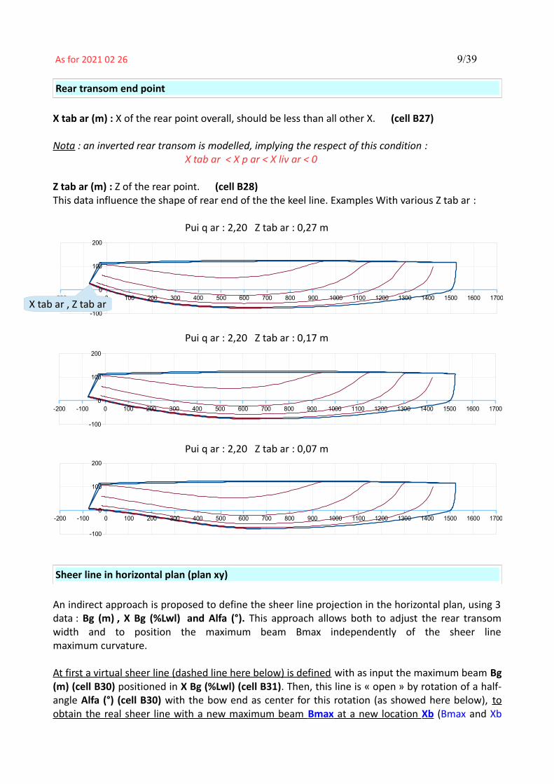
Rear transom end point

X tab ar (m) : X of the rear point overall, should be less than all other X. (cell B27)

Nota : an inverted rear transom is modelled, implying the respect of this condition :X tab ar < X p ar < X liv ar < 0

Z tab ar (m) : Z of the rear point. (cell B28)This data influence the shape of rear end of the the keel line. Examples With various Z tab ar :

Pui q ar : 2,20 Z tab ar : 0,27 m

Pui q ar : 2,20 Z tab ar : 0,17 m

Pui q ar : 2,20 Z tab ar : 0,07 m

Sheer line in horizontal plan (plan xy)

An indirect approach is proposed to define the sheer line projection in the horizontal plan, using 3data : Bg (m) , X Bg (%Lwl) and Alfa (°). This approach allows both to adjust the rear transomwidth and to position the maximum beam Bmax independently of the sheer linemaximum curvature.

At first a virtual sheer line (dashed line here below) is defined with as input the maximum beam Bg(m) (cell B30) positioned in X Bg (%Lwl) (cell B31). Then, this line is « open » by rotation of a half-angle Alfa (°) (cell B30) with the bow end as center for this rotation (as showed here below), toobtain the real sheer line with a new maximum beam Bmax at a new location Xb (Bmax and Xb

-200 -100 0 100 200 300 400 500 600 700 800 900 1000 1100 1200 1300 1400 1500 1600 1700

-100

0

100

200

X tab ar , Z tab ar

-200 -100 0 100 200 300 400 500 600 700 800 900 1000 1100 1200 1300 1400 1500 1600 1700

-100

0

100

200

-200 -100 0 100 200 300 400 500 600 700 800 900 1000 1100 1200 1300 1400 1500 1600 1700

-100

0

100

200

As for 2021 02 26 10/39

being computed by the system and showed in blue opposite to the input data). So a set of valuesfor Bg, X Bg and Alfa leads to the real sheer line with maximum beam Bmax at a real position Xb.By doing so, the sheer line maximum curvature remains close to X Bg and is disconnected to

Nota : this « Alfa » reshaping of the hull is powerful, it can be done at any moment of the hulldefinition, all the stations and waterlines are automatically updated.

Example 1 :

Bg = 0,8 m ; X Bg = 50 % Lwl ; Alfa = 0° >>> generic hull

… + rotation Alfa = 2° >>> real hull with Bmax = 1,42 m at Xb = 34 %Lwl

The generic hull can be virtual but yet be transformed into a real one by application of a greatenough Alfa >>> Exemple 2 :

Bg = 0,4 m ; X Bg = 65 %Lwl ; Alfa = 0° >>> (virtual) generic hull !!!

… but with a rotation Alfa = 4° >>> Real hull Bmax = 1,54 m at Xb 27 % Lwl

In each case the maximum curvature of the sheer line remains close to X Bg of the generic hull :>>> Example 1 : 50% Lwl ; Example 2 : 65 % Lwl

-200 -100 0 100 200 300 400 500 600 700 800 900 1000 1100 1200 1300 1400 1500 1600 1700

-100,00

0,00

100,00

-200 -100 0 100 200 300 400 500 600 700 800 900 1000 1100 1200 1300 1400 1500 1600 1700

-100,00

0,00

100,00

-200 -100 0 100 200 300 400 500 600 700 800 900 1000 1100 1200 1300 1400 1500 1600 1700

-100,00

0,00

100,00

-200 -100 0 100 200 300 400 500 600 700 800 900 1000 1100 1200 1300 1400 1500 1600 1700

-100,00

0,00

100,00

Bmax at Xb Maxi curvature remains at ~ X Bg

Centre of the rotation Alfa

Bg at X Bg

-200 -100 0 100 200 300 400 500 600 700 800 900 1000-150

-100

-50

0

50

100

150

As for 2021 02 26 11/39

Pui liv y, Cor Pui liv and Pui Cor Pui are 3 adimensional coefficients for respectively the power ofthe sheer line polynomial, its correction along with x and the power of the correction polynomialitself (formulation details in the technical appendix).

Pui liv y (cell B33) : Pui liv y = 2 gives the better curvature regularity in the midship zone, it is the recommendedvalue. Pui liv < 2 lead to a more accentuated curvature (up to a folding when Pui liv < 1,5) and onthe other hand a Pui liv > 2 lead to a flattening in the midship zone. Examples :

Pui liv y = 1,7 :

Pui liv y = 2 :

Pui liv y = 2,5 :

… up to a « barge » like shape when using Pui liv y = 3 :

Cor Pui liv (cell B34) can add more or less tension towards the front anf aft ends of the sheer line,meaning ends with less curvature. Examples :

-200 -100 0 100 200 300 400 500 600 700 800 900 1000 1100 1200 1300 1400 1500 1600 1700

-100,00

0,00

100,00

-200 -100 0 100 200 300 400 500 600 700 800 900 1000 1100 1200 1300 1400 1500 1600 1700

-100,00

0,00

100,00

-200 -100 0 100 200 300 400 500 600 700 800 900 1000 1100 1200 1300 1400 1500 1600 1700

-100,00

0,00

100,00

-200 -100 0 100 200 300 400 500 600 700 800 900 1000 1100 1200 1300 1400 1500 1600 1700

-100,00

0,00

100,00

As for 2021 02 26 12/39

Cor Pui liv = 0

>>> Cor Pui liv = 0,05

Negative values of Cor Pui Liv can be tested too, with the inverted effect.

Pui Cor Pui (cell B35) acts on the application with x of the correction Cor Pui liv. Pui Cor Pui < 1 >>> distributes the correction over the entire lengthPui Cor Pui =1 >>> correction application is linear with length XPui Cor Pui > 1 >>> amplifies the correction towards the ends.

Some examples :

Pui Cor Pui = 0,5 (with Cor Pui liv = 0,05)

>>> Pui Cor Pui = 2 (with Cor Pui liv = 0,05)

-200 -100 0 100 200 300 400 500 600 700 800 900 1000 1100 1200 1300 1400 1500 1600 1700

-200,00

-100,00

0,00

100,00

200,00

-200 -100 0 100 200 300 400 500 600 700 800 900 1000 1100 1200 1300 1400 1500 1600 1700

-200,00

-100,00

0,00

100,00

200,00

-200 -100 0 100 200 300 400 500 600 700 800 900 1000 1100 1200 1300 1400 1500 1600 1700

-200,00

-100,00

0,00

100,00

200,00

-200 -100 0 100 200 300 400 500 600 700 800 900 1000 1100 1200 1300 1400 1500 1600 1700

-200,00

-100,00

0,00

100,00

200,00

As for 2021 02 26 13/39

>>> Pui Cor Pui = 4 , up to unusual shape ! (with Cor Pui liv = 0,05)

Nota : with recommended values of 0,5 to 2, Pui Cor Pui acts as a fine tuning of the tensioning ofthe ends of the sheer line triggered by Cor Pui liv.

X liv ar (m) (Cell B36) : it is the X position of the rear point of the sheer line (see Fig. 1 page 8).Condition to fullfil : X liv ar < 0 and > X p ar. X liv ar is the position taken for the draw of the stationnamed Car 1 .

Nota : Y value of the sheer line aft point is not specified, as it results from the 6 previousparameters here above detailed.

Scow (Cell B37) : it is a coefficient introducing a scow influence on the bow shape of the sheer line.Scow = 0 to 1 ; 0 = no scow bow ; 1 = full « rectangular » size scow bow

Example with Scow = 0,2



-200 -100 0 100 200 300 400 500 600 700 800 900 1000 1100 1200 1300 1400 1500 1600 1700

-200,00

-100,00

0,00

100,00

200,00

-200 -100 0 100 200 300 400 500 600 700 800 900 1000 1100 1200 1300 1400 1500 1600 1700

-200,00

-100,00

0,00

100,00

200,00

-200 -100 0 100 200 300 400 500 600 700 800 900 1000 1100 1200 1300 1400 1500 1600 1700

-200,00

-100,00

0,00

100,00

200,00

-200 -100 0 100 200 300 400 500 600 700 800 900 1000 1100 1200 1300 1400 1500 1600 1700

-200,00

-100,00

0,00

100,00

200,00

As for 2021 02 26 14/39

Option Hard chine line, its definition in the vertical projection (xz plan)

Type : 0 = no hard chine ; 1 = hard chine defined by 2 heights and a power of polynome ;2 = hard chine defined by 3 heights ;

When Type = 1 , two data to input :1,2 Zhc av (m): height of the hard chine line at the bow (cell B40)1,2 Zhc ar (m) : height of the hard chine line at the aft (cell B42)

When Type = 2, a third height is to input :2 Zhc m (m) : height of the hard chine line at 35% Lwl (cell B41)

Pui hc z : power of the polynomial defining the hard chine line of Type 1, should be ≥ 1 (cell B43)

Example Type 1 (2 points) with Zhc av = 0,24 m ; Zhc ar = 0,50 m ; Pui hc z = 1

Example Type 2 (3 points) with Zhc av = 0,4 m ; Zhc m = 0,20 m ; Zhc ar = 0,5 m

Sheer line, its definition in vertical projection (xz plan)

Z liv m (m) : it is the freeboard at 35% Lwl (cell B45)Z liv ar (m) : it is the aft freeboard, specified at the sheer line aft point. (cell B46)

-200 -100 0 100 200 300 400 500 600 700 800 900 1000 1100 1200 1300 1400 1500 1600 1700

-400

-300

-200

-100

0

100

200

Zhc av

-200 -100 0 100 200 300 400 500 600 700 800 900 1000 1100 1200 1300 1400 1500 1600 1700

-400

-300

-200

-100

0

100

200

Zhc mZhc ar Zhc av

Zhc ar

As for 2021 02 26 15/39

Together with Z bow defined here before, these are the 3 freeboards on which leans the xzpolynomial for the sheer line definition. Example :

Another example, here with Z liv m > Z bow

Hull deck / central line of symmetry

Athough not a definitive feature for a catamaran design, a deck surface for each hull is proposed,made of transversal circular arcs based on both the sheer line definition and the central line ofsymmetry (at y = 0) going from the front end of the hull (X bow, Z bow) and defined by :

– a point at midship : Zp m (m) at X = 35% Lwl (cell B48)– a point at the rear end of the deck : Xp ar (m) , Zp ar (m) (cells B49 & B50)

Example :

-200 -100 0 100 200 300 400 500 600 700 800 900 1000 1100 1200 1300 1400 1500 1600 1700

-100

0

100

200

Z bowZ liv mZ liv ar

-150 -100 -50 0 50 100 150 200 250 300 350 400 450 500 550 600 650 700 750 800 850 900 950

-50

0

50

100

Z bowZp mXp ar , Zp ar

-200 -100 0 100 200 300 400 500 600 700 800 900 1000 1100 1200 1300 1400 1500 1600 1700

-100

0

100

200

As for 2021 02 26 16/39

Sections

Sections are defined through using a generalised « E » formulation, « E » for Elliptical but thegeneralised formulation allows a wide variety of shape, here some typical examples :

E sections adimensional parameters :

Two parameters Pui E1 and Pui E2 are to be input, eazch at fore, mid and aft location. Examples :

(Cells B52 to 54) (Cells D52 to 54)

-150 -100 -50 0 50 100 150

-100

-50

0

50

100

150

-150 -100 -50 0 50 100 150

-100

-50

0

50

100

150

-150 -100 -50 0 50 100 150

-100

-50

0

50

100

150

-150 -100 -50 0 50 100 150

-100

-50

0

50

100

150

-150 -100 -50 0 50 100 150

-100

-50

0

50

100

150

-150 -100 -50 0 50 100 150

-100

-50

0

50

100

150

-150 -100 -50 0 50 100 150

-100

-50

0

50

100

150

-150 -100 -50 0 50 100 150

-100

-50

0

50

100

150

-150 -100 -50 0 50 100 150

-100

-50

0

50

100

150

Pui E1 fore 1,20 Pui E2 fore 2,00 at XbowPui E1 mid 0,79 Pui E2 mid 3,04 at C5Pui E1 aft 0,65 Pui E2 aft 2,53 at X tab ar

As for 2021 02 26 17/39

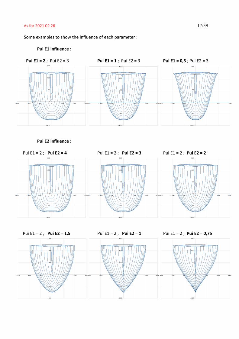
Some examples to show the influence of each parameter :

Pui E1 influence :

Pui E1 = 2 ; Pui E2 = 3 Pui E1 = 1 ; Pui E2 = 3 Pui E1 = 0,5 ; Pui E2 = 3

Pui E2 influence :

Pui E1 = 2 ; Pui E2 = 4 Pui E1 = 2 ; Pui E2 = 3 Pui E1 = 2 ; Pui E2 = 2

Pui E1 = 2 ; Pui E2 = 1,5 Pui E1 = 2 ; Pui E2 = 1 Pui E1 = 2 ; Pui E2 = 0,75

-150 -100 -50 0 50 100 150

-100

-50

0

50

100

150

-150 -100 -50 0 50 100 150

-100

-50

0

50

100

150

-150 -100 -50 0 50 100 150

-100

-50

0

50

100

150

-150 -100 -50 0 50 100 150

-100

-50

0

50

100

150

-150 -100 -50 0 50 100 150

-100

-50

0

50

100

150

-150 -100 -50 0 50 100 150

-100

-50

0

50

100

150

-150 -100 -50 0 50 100 150

-100

-50

0

50

100

150

-150 -100 -50 0 50 100 150

-100

-50

0

50

100

150

-150 -100 -50 0 50 100 150

-100

-50

0

50

100

150

As for 2021 02 26 18/39

Example with Pui E1 = 0,5 which, associated with a hard chine line, can give a spray rail :

A last recommendation on input data for the hull :Probably that the use of the adimensional parameters are not always very intuitive at thebeginning :

– the ones of hull of reference data are there to guide in your first steps,– you can test the effect of each parameter, including by testing a priori very low or very high

values so that to better see the effects, and this « learning by testing » process will help youto progress rapidly.

-150 -100 -50 0 50 100 150

-100

-50

0

50

100

150

As for 2021 02 26 19/39

1.2 Daggerboard data

Data to enter are in column B , cells B56 to B64 :

C root

Xq ar (m) 7,50C root (m) 0,70

C roundness 4,00t/c (%) 14,00

Draft oa (m) 2,80naca 00xx 0

naca 63-0xx 1naca 65-0xx 0

Density 0,55

t/c %

Draft oa

-200 -100 0 100 200 300 400 500 600 700 800 900 1000 1100 1200 1300 1400 1500 1600 1700

-400

-300

-200

-100

0

100

200

C roundness

Rear point of the root chordRoot chord length

Relative thickness of the profileshould be > hull draft TcType of profile (in the horizontal plans)Put 1 for the profile used, 0 for the others

Roudness of the profile lower part ; should be usually 2,5 to 5,5

Xq ar

Draft oa

-150 -100 -50 0 50 100 150

-350

-300

-250

-200

-150

-100

-50

0

50

100

150

t/c %

As for 2021 02 26 20/39

1.3 Rudder data

Data to enter are in column B , cells B66 to B74 :

As for the keel, data to enter allow the geometrical definition of the longitudinal profile of therudder and the naca profiles used at various horizontal sections.

Naca 00xx Naca 63-0xx Naca 65-0xx

0 1 0

Ex : Profil Naca 63-0xx with Th max at 35% c >>>

Nota : daggerboard and rudder profiles are calculated and drawn with a cut-off at 97,5% c so toavoid trailing edges too tapered and unfeasible. Computed chord c are equal to C/0,975, C beingthe geometrical chords.

Xr ar C root

R angle

Zr arC roundness

Xr ar (m) 0,00C root (m) 0,40

t/c (%) 15,00R angle (°) 85,00

L ar (m) 1,60C roundness 3,50

naca 00xx 0naca 63-0xx 1naca 65-0xx 0

Rear point of the root chordRoot chord lengthRelative thickness of the profileRudder rear angle, should be around 80°-85°Rudder rear span

Type of profile (in the horizontal plans)Put 1 for the profile used, 0 for the others

Roudness of the profile lower part ; should be usually 2,5 to 5,5

t/c %

As for 2021 02 26 21/39

Storage of Gene-Hull input data : the spreadsheet includes a second sheet called « Hulls storage »where you can store by copy/paste the input data in column B & D, for your various projects orvariants of a hull during the iteration process. The hull C1 given as example is stored here too :

Input for C11.1 Hull data metric >> feet

Lwl (m) 15,00 49,21Beam between hulls axis

Bhu (m) 6,10 20,01

Tc (m) 0,77 2,53X Tc (%Lwl) 45,0

Xbow (m) 15,25 50,03Zbow (m) 1,15 3,77

Cet 90Polynomials of the keel line, front part and rear part :

Pui q av 2,20Pui q ar 2,20

X tab ar (m) -0,75 -2,46Z tab ar (m) 0,170 0,56

Bg (m) 0,80 2,62X Bg (% Lwl) 56,5

Alfa (°) 3,90Pui liv y 2,00

Cor Pui liv 0,020Pui Cor Pui 1,00X liv ar (m) -0,20 -0,66

Scow 0,10

Type 11,2 Zhc av (m) 0,24 0,79

2 Zhc m (m) 0,65 2,131,2 Zhc ar (m) 0,5 1,64

Pui hc z 1

Z liv m (m) 1,2 3,94Z liv ar (m) 1,10 3,61

Deck / central line rear end Z p m (m) 1,25 4,10X p ar (m) -0,30 -0,98Z p ar (m) 1,15 3,77

Pui E1 av 1,20 Pui E2 av 2,00Pui E1 mid 0,79 Pui E2 mid 3,04

Pui E1 ar 0,65 Pui E2 ar 2,531.2 Daggerboard

Xq ar (m) 6,90 22,64C root (m) 0,70 2,30

C roundness 4,00t/c (%) 14,00

Draft oa (m) 2,80 9,19naca 00xx 1

naca 63-0xx 0naca 65-0xx 0

Density 0,551.3 Rudder data

Xr ar (m) 0,00 0,00C root (m) 0,40 1,31

t/c (%) 15,00R angle (°) 85,00

L ar (m) 1,60 5,25C roundness 3,50

naca 00xx 0naca 63-0xx 1naca 65-0xx 0

Lenght of waterline :

Maximum draft of the hull body :

Hull bow :

Shape coefficient of the bow :

Rear end of the transom :

Sheer line, in horizontal projection xy :

Option Hard Chine line, in vertical projection xz :

Sheer line, in vertical projection xz :

Sections « E » shape (E like Elliptic) sections

As for 2021 02 26 22/39

Gene-Hull sheet / output

A hull with fairing lines and hydrostatic characteristics is automatically produced as long as all dataare fulfilled with consistent values. Modification of one value leads in real time to an updatedversion of the hull (drawings and other ouput computations).

These output are divided into several sections 2 to 7, the User should act in some of them foreither change and fix the scale of the views or introduce some complementary data for specificstudy (the heel angle, etc …)

2. Data sum-up and results of hydrostatic and surfaces calculations

These data and results are autmatically produced, no intervention by the User.

They include parameters and ratios usually considered by naval architects to judge the consistenceof the hull design, inc. the ones in red which are more specifically relevant for a catamaran :

– Lwl / D^(1/3) (in metric units), its translation in DLR (in lbs,feet units)– Lwl/Bwl , Bwl/Tc– Space hulls axis : S/Lwl– Displacements at waterline H0 (i.e. as drawn)– Xc (LCB) and Zc positions of the center of buoyancy – Cp (Prismatic coefficient) of the hull– Sf (floatation aera) and its longitudinal center– Sw (hull wetted surface) – Daggerboard and rudder volume, lateral surface and wetted surface– …..

… + the curve of the sections aeras, for waterline H0,

… + to contribute to the mass balance data :– Shull (surface of the hull) , its center of gravity position X,Z – Sdeck (surface of the deck for each hull), its center of gravity position X

...+ center of lateral resistance CLR (according to Larsson-Eliasson method for fin keel, here thedaggerboard).

…+ the recopy of the data coming from the mass spreadsheet : boat light weight and CoG location.

As for 2021 02 26 23/39

Example for C1 :

Hull design and mass should be adjusted so that Displacement (kg) = M (kg), and LCB (m) equal orclose to Xg (m) .

2. Data sum-up and results of hydrostatic and surfaces calculations2.1 Hull Loa (m) 16,00 Lwl (m) 15,00

>> ft 52,49 49,21Bhull (m) 1,97 at X (% Lwl) 31,0 Boa (m) 8,07 Space hulls axis (m) 6,10

>> ft 6,47 >> ft 26,48 > S/Lw 0,41Bwl (m) 1,60 at X (% Lwl) 39,0 > Lwl / Bwl 9,35

>> ft 5,26 Freeboards (m) > Aft Midship ForeTc (m) 0,77 at X (%Lwl) 45,0 > Bwl / Tc 2,08 1,1 1,20 1,15

>> ft 2,53 >> ft 3,61 3,94 3,77Displacement at H0 (m3) 7,70072 at LCB (m) 6,893 LCB (%Lwl) 45,95 Zc (m) -0,280

>> lbs 17401 w. seawater 1025 kg/m3 >> ft -0,92Cp 0,565 > Lwl/D^(1/3) 7,60

Sf (m2) 17,56 at Xf (m) 6,674 Xf (%Lwl) 44,49 >>> Xc – Xf (%Lwl) 1,46>> ft2 188,99 >> ft 21,90

Sw (m2) 25,40 >Sm/D^(2/3) 6,51>> ft2 273,36

Shull (m2) 64,52 at X (m) 7,102 Z (m) 0,185>> ft2 694,51 >> ft 23,30 >> ft 0,61

Sdeck (m2) 23,38 at X (m) 6,224>> ft2 251,64 >> ft 20,42

2.2 DaggerboardVol. (m3) 0,06612 at X (m) 7,243 X (%Lwl) 48,29 Z (m) -1,550

Mass (kg) 36,36 >> ft 23,76 >> ft -5,09>> lbs 80

Draft oa (m) 2,80 Sw (m2) 2,37 Sxz (m2) 1,14>> ft 9,19 >> ft2 25,49 >> ft2 12,25

CLR (m) 7,37 CLR (%Lwl) 49,10 CLR = Center of Lateral Resistance>> ft2 79,28

2.3 RudderVolume (m3) 0,01904 at X (m) 0,154 X (%Lwl) 1,03 Z (m) -0,732

Sw (m2) 1,15 >> ft 0,51 Sxz (m2) 0,55 per rudder>> ft2 12,33 >> ft2 5,93

Loa (m) 16,00 Boa (m) 8,07>> ft 52,49 >> ft 26,48

Displacement at H0 (m3) 15,57176 at LCB (m) 6,879 LCB (%Lwl) 45,86 Zc (m) -0,291(kg) 15961 >> ft 22,57 >> ft -0,96

>> lbs 35188Sw (m2) 57,82 >Sw/D^(2/3) 9,27 Lwl/D^(1/3) 6,01

>> ft2 622,36 DLR 132 M(lbs/2240)/(Lwl(ft)/100)^32.5 Data from the mass spreadsheet

M (kg) 15961 at Xg (m) 6,900 Xc (%Lwl) 46,00 at Zg (m) 2,137

method : daggerboard profile extended to the waterline, LCR at 25% chord and 45% draft oa

2.4 Catamaran : 2 Hulls + 2 Daggerboards + 2 Rudders

Light boat:

As for 2021 02 26 24/39

3. The 3 views 2D

The views are automatically redrawn after every input data modification.

View of the front sections include sections ≥ C4 (= 40% Lwl), with a half section pitch : C4, C4,5, C5,.... In front of C10 (Front perpendicular), 2 complementary sections Cav1 and Cav2 are drawn, at1/3 and 2/3 of the bow overlenght. View of the rear sections includes sections ≤ C4, with a half section pitch : C4, C3,5, C3, C2,5, …Behind C0, 2 complementary sections Car1 and Car2 are drawn, Car2 at the rear end point of thesheer line and Car1 at the middle point between this rear point and C0. And the rear transom isalso computed and drawn in this view (as long as it is an inverted one within the condition : X tabar < X pont ar < X liv ar < 0).

In the plan view of the bottom, waterlines in red are the wetted ones, the thick red line being thewaterline H0.

User intervention : axis scales are proposed automatic, grid pitch fixed and equal for the 2coordinates. As long as the project dimensions are fixed , it is recommended to modify (ifnecessary) and to fix the scale of the views for orthonormal views (i.e. square grid).

Example :

-200 -100 0 100 200 300 400 500 600 700 800 900 1000 1100 1200 1300 1400 1500 1600 1700

-400

-300

-200

-100

0

100

200

-150 -100 -50 0 50 100 150

-350

-300

-250

-200

-150

-100

-50

0

50

100

150

-150 -100 -50 0 50 100 150

-350

-300

-250

-200

-150

-100

-50

0

50

100

150

As for 2021 02 26 25/39

4. Curves of control

These curves are proposed to assess some complementary characteristics of the hull : – Waterlines angles in the horizontal plan xy, with the same color code blue/red as for the

bottom view. – Curvature 1/R of :

– Waterlines and sheer line (in the horizontal plan xy) with idem color code blue/red,– Keel line and Buttocks lines (vertical longitudinal cuts) in green, keel line being the thick

one – Check of the Pui E1 and Pui E2 values with X (the parameters to define the sections shape)

Examples :

-200 -100 0 100 200 300 400 500 600 700 800 900 1000 1100 1200 1300 1400 1500 1600 1700

-200,00

-100,00

0,00

100,00

200,00

-200 -100 0 100 200 300 400 500 600 700 800 900 10001100120013001400150016001700

-20

-10

0

10

20

30

40

Angles (°) of the water lines (in horizontal projection xy)

Red : below H0 (thick line = H0) ; Blue : above H0 (thick line = sheer line)

Bow entry half anglehere < 10°

As for 2021 02 26 26/39

-200 -100 0 100 200 300 400 500 600 700 800 900 1000 1100 1200 1300 1400 1500 1600 17000,0

0,1

0,2

Curvature 1/R

Red : waterlines below H0 (thick line = H0) ; Blue : waterlines above H0 (thick line = sheer line) Green : keel and buttock lines (Thick line = keel line)

-200 -100 0 100 200 300 400 500 600 700 800 900 1000 1100 1200 1300 1400 1500 1600 17000,0

0,2

0,4

0,6

0,8

1,0

1,2

1,4

Check : PE1 for "E" sections (red points = input values)

As for 2021 02 26 27/39

5. Stability and righting moment with a loading

In this section, you can : – input a loading (weight and location) and see the consequence on the upright hydrostatics

data (when heel = 0°)– estimate the transversal GM (from the equilibrium at heel = 1°) >> GM1°– compute the equilibrium for any heel angle up to the windward hull off the water, with

output including the trim , the % of displacement of each hull, the righting moment, thewetted surface Sw, etc …

– to prepare data for « SA-VPP Catamaran » dedicated to a sailing catamaran

In the design loop, it is the step 4 , to do after step 1 (Hull and appendages generation), step 2(Sailplan, see here after) and step 3 (Mass spreadsheet, see here after), and before step 5(performance estimation with SA-VPP catamaran) . An example of this design loop is given in theexample document for the catamaran C1.

In the section 5.1, a design loading can be introduced : the User input data for a load and itslocation (in the yellow cells) , here below an example :

Load = 600 kgXg = 4,0 mYg = 0 m & Zg 2,0 m (Crew at center) and Yg = 3,0 m & Zg 2,0 m (Crew sit windward)

-200 -100 0 100 200 300 400 500 600 700 800 900 1000 1100 1200 1300 1400 1500 1600 17000,0

0,5

1,0

1,5

2,0

2,5

3,0

3,5Check : PE2 for "E" sections (red points = input values)

5.1 Mass spreadsheet with input of a load

As for 2021 02 26 28/39

The data in the grey cells comes from the mass spreadsheet (see here after). The resulting data (indark red) are used in the computation of the hydrostatic equilibrium in the sub-section 5,2.

The User can input an heel angle and iterates on height and trim up to reach the « hydrostatics »equilibrium, i.e. both weight = displacement and Xc (LCB) = Xg.

>>> the user should iterate on the values of Height and Trim up to :– Displacement with heel = Displacement from the mass spreadsheet– Xc heel = Xg

This sub-routine can be used for various investigations :

The case Heel = 0° inform on the draft and trim for the given loading. Example :

The results are given for each hull and for the 2 hulls where the equilibrium could be checked :In the example above, for the loading 600 kg and at heel 0°, the sinkage is 1,6 cm together with aslight nose-up trim of 0,16° (Trim > 0 = nose-up) . Each hull have a Lwl of 15,32 m.

4,00,54570,062

Data to enterHeel (°)

Height (cm)Trim (°)

Results for the 2 hullsDisp. (m3) 16,15710 / Disp. (m3) 16,15711

Xc heel (m) 6,795 / Xg (m) 6,795

and to to compare with :

To input

To input and to iterate … … up to equilibrium

Data to enter Results for leeward hull Results for windward hull Results for the 2 hullsHeel (°) 0,0 %Disp 0,50 %Disp 0,50 Disp. (m3) 16,15712 / Disp. (m3) 16,15711

Height (cm) -1,5933 Disp. (m3) 8,07856 Disp. (m3) 8,07856 Xc heel (m) 6,795 / Xg (m) 6,795Trim (°) 0,155 Xc heel (m) 6,795 Xc heel (m) 6,795 Other results

Other results Other results Yc heel (m) 0,000 Hull Mom(m4) 0,000Yc heel (m) -3,050 Yc heel (m) 3,050 Zc heel (m) -0,297 Mom(kN.m) 0,00Zc heel (m) -0,297 Zc heel (m) -0,297 Sw (m2) 59,34 Yg heel (m) 0,109

Sw (m2) 29,67 Sw (m2) 29,67 GZ (m) 0,109Sf (m2) 17,82 Sf (m2) 17,82 RM (kN.m) 17,66Lwl (m) 15,32 Lwl (m) 15,32 Relevant only at Heel = 1° equilibriumBwl (m) 1,62 Bwl (m) 1,62 Yg heel (m) 0,000 with crew at centerTc (m) 0,79 Tc (m) 0,79 Gz (m) 0,000

Cp 0,563 Cp 0,563 >> GM1° (m) 'Put Heel 1°LCB (%Lw) 46,4 LCB (%Lw) 46,4

Lwl/Bwl 9,46 Lwl/Bwl 9,46Bwl/Tc 2,06 Bwl/Tc 2,06

Lwl/D^1/3 7,63 Lwl/D^1/3 7,63


GZ & RM (Crew sit windward)

Mass Xg Zg Yg (in the coordinates of the 2D plan views above)(kg) (m) (m) (m)

Boat light weight (kg) 15961,04 6,900 2,137 0 from the mass spreadsheetLoad (kg) 600,00 4,00 2,00 0,00 Crew at center

2,00 3,00 Crew sit windwardTotal >>> Mass (kg) 16561,04 6,795 2,132 0,000 Crew at center

Disp. (m3) 16,15711 2,132 0,109 Crew sit windward

Data to enter : yellow cells

5.2 Computation : input of an Heel angle and iteration on Height and Trim up to Displacement equality and Xc (LCB) = Xg

As for 2021 02 26 29/39

The case Heel = 1° give the metacentric center GM1° representative of the initial stability whenthe loading is Y-centered (the pink results are with Yg = 0) . Example :

>>> Here, the relevant result is in pink : GM1° = 18,41 m

The case Heel = 4° can give the catamaran attitude and the RM for an usual sailing. Example :

>>> in this example : the displacement repartition is 0,73 D for the leeward hull and 0,27 D for thewindward hull. In blue are all the other output data for each hull. The overall righting moment RMis 219 kN.m and the overall wetted surface Sw is 57,85 m2. The trim is 0,06°.


Height (cm) -1,4481 Disp. (m3) 9,02428 Disp. (m3) 7,13283 Xc heel (m) 6,795 / Xg (m) 6,795Trim (°) 0,145 Xc heel (m) 6,776 Xc heel (m) 6,820 Other results

Other results Other results Yc heel (m) -0,358 Hull Mom(m4) 5,791Yc heel (m) -3,051 Yc heel (m) 3,048 Zc heel (m) -0,298 Mom(kN.m) 58,23Zc heel (m) -0,314 Zc heel (m) -0,278 Sw (m2) 59,17 Yg heel (m) 0,071

Sw (m2) 31,54 Sw (m2) 27,63 GZ (m) 0,430Sf (m2) 18,61 Sf (m2) 16,84 RM (kN.m) 69,84Lwl (m) 15,90 Lwl (m) 14,62 Relevant only at Heel = 1° equilibriumBwl (m) 1,66 Bwl (m) 1,57 Yg heel (m) -0,037 with crew at centerTc (m) 0,84 Tc (m) 0,73 Gz (m) 0,321

Cp 0,555 Cp 0,574 >> GM1° (m) 18,41LCB (%Lw) 47,3 LCB (%Lw) 44,1


Lwl/D^1/3 7,64 Lwl/D^1/3 7,59




Height (cm) 0,5457 Disp. (m3) 11,75836 Disp. (m3) 4,39874 Xc heel (m) 6,795 / Xg (m) 6,795Trim (°) 0,062 Xc heel (m) 6,751 Xc heel (m) 6,913 Other results

Other results Other results Yc heel (m) -1,388 Hull Mom(m4) 22,432Yc heel (m) -3,041 Yc heel (m) 3,030 Zc heel (m) -0,324 Mom(kN.m) 225,56Zc heel (m) -0,362 Zc heel (m) -0,222 Sw (m2) 57,85 Yg heel (m) -0,040


Cp 0,583 Cp 0,576 >> GM1° (m) 'Put Heel 1°LCB (%Lw) 46,9 LCB (%Lw) 44,1


Lwl/D^1/3 7,04 Lwl/D^1/3 8,01



As for 2021 02 26 30/39

>>> for this heel angle, the rear transom bottom end is just at the level of the water.

-500 -400 -300 -200 -100 0 100 200 300 400 500

-400

-300

-200

-100

0

100

200

300

-500 -400 -300 -200 -100 0 100 200 300 400 500

-400

-300

-200

-100

0

100

200

300

As for 2021 02 26 31/39

You can go up to the case for which the windward hull is fully off the water, here with Heel = 12°Example :

>>> The RM is then at its maximum, here 416,9 kN.m and the Sw is 43,25 m2. The rear transom ispartly immersed.

-100 0 100 200 300 400 500 600 700 800 900 1000 1100 1200 1300 1400 1500 1600

-500

-400

-300

-200

-100

0

100

200

300

400

500


Height (cm) 21,3907 Disp. (m3) 16,07197 Disp. (m3) 0,08516 Xc heel (m) 6,795 / Xg (m) 6,795Trim (°) -0,425 Xc heel (m) 6,801 Xc heel (m) 5,648 Other results

Other results Other results Yc heel (m) -2,903 Hull Mom(m4) 46,654Yc heel (m) -2,918 Yc heel (m) 0,000 Zc heel (m) -0,435 Mom(kN.m) 469,12Zc heel (m) -0,432 Zc heel (m) -1,124 Sw (m2) 43,25 Yg heel (m) -0,337


Cp 0,619 Cp #DIV/0 ! >> GM1° (m) 'Put Heel 1°LCB (%Lw) 47,2 LCB (%Lw) #DIV/0 !

Lwl/Bwl 8,39 Lwl/Bwl #DIV/0 !Bwl/Tc 1,62 Bwl/Tc #DIV/0 !

Lwl/D^1/3 6,34 Lwl/D^1/3 0,00



As for 2021 02 26 32/39

-500 -400 -300 -200 -100 0 100 200 300 400 500

-400

-300

-200

-100

0

100

200

300

-500 -400 -300 -200 -100 0 100 200 300 400 500

-400

-300

-200

-100

0

100

200

300

As for 2021 02 26 33/39

In the table proposed in this sub-section, all the necessary data for « SA-VPP Catamaran »spreadsheet application are gathered and, once fulfilled, the table can be copy/special paste intothe SA-VPP file.

One can see that some cells are automatically fulfilled and some others are to be fulfilled by theUser : they concern the data of each hul for 3 heel angles in order to cover the usual range ofangles for a cruise sailing. The first heel angle should be 0, the third heel angle could be the onejust before the emergence of the windward hull, and the second angle an intermediate value. Herefor the example, we choose 0°, 4° and 8° . The process is to set the heel angle and iterates up tothe equilibrium (as described in the 5.2 here above) and then the hulls data for the table areautomatically duplicated above the table. The following is then :

-100 0 100 200 300 400 500 600 700 800 900 1000 1100 1200 1300 1400 1500 1600

-500

-400

-300

-200

-100

0

100

200

300

400

500

5.3 Data preparation for SA-VPP Catamaran

Heel (°) Lwl (m) Bwl (m) Tc (m) Cp LCB (%Lwl) Sf (m2) Sw tot (m2) Disp. (m3) RM (kN.m)Lee Hull

Wind HullLee Hull

Wind HullLee Hull

Wind HullEach daggerboard Each rudder Hull beam Hulls axis space

Vol. (m3) Sw (m2) Chord (m) Draft (m) Vol. (m3) Sw (m2) Chord (m) Boa (m) Space (m)0,06612 2,37 0,70 2,80 0,01904 1,15 0,40 1,97 6,10

AdjustmentsSA (m2) ZCE (m) Zdeck (m) Zmast (m) Main (m2) Spi (m2) ZCE spi (m) Reefing Flat mini Windward daggerboard147,15 9,11 1,15 22,72 81,50 229,78 10,54 1,00 0,5 1,0

For SA-VPP

From the Sailplan sheet :

As for 2021 02 26 34/39

Heel = 0° and equilibrium done within 5.2 >>> :

, then the User can copy/special paste (number, format) the data in the table :

Heel 4° and equilibrium done within 5.2 >>> :


Heel 8° and equilibrium done within 5.2 >>> :


Heel (°) Lwl (m) Bwl (m) Tc (m) Cp LCB (%Lwl) Sf (m2) Sw (m2) Disp. (m3) RM (kN.m)Lee Hull 0,0 15,32 1,62 0,79 0,563 46,4 17,82 29,67 8,079 17,658

Wind Hull 0,0 15,32 1,62 0,79 0,563 46,4 17,82 29,67 8,079

Lines of data generated at each equilibrium, to copy/special paste (Number, Format) in the table here below :

Heel (°) Lwl (m) Bwl (m) Tc (m) Cp LCB (%Lwl) Sf (m2) Sw tot (m2) Disp. (m3) RM (kN.m)Lee Hull 0,0 15,32 1,62 0,79 0,563 46,4 17,82 29,67 8,079 17,658

Wind Hull 0,0 15,32 1,62 0,79 0,563 46,4 17,82 29,67 8,079Lee Hull

Wind HullLee Hull




For SA-VPP



Wind Hull 4,0 13,13 1,42 0,56 0,576 44,1 13,73 21,60 4,399



Wind Hull 0,0 15,32 1,62 0,79 0,563 46,4 17,82 29,67 8,079Lee Hull 4,0 16,00 1,77 0,98 0,583 46,9 20,50 36,26 11,758 219,024

Wind Hull 4,0 13,13 1,42 0,56 0,576 44,1 13,73 21,60 4,399Lee Hull




For SA-VPP



Wind Hull 8,0 9,90 1,12 0,29 0,602 44,5 8,34 13,01 1,397


As for 2021 02 26 35/39

>>> The table is fullfilled and ready to be itself copy/special paste (text, number, format) into SA-VPP Catamaran file

Sailplan input and ouput

This sheet can provide an early stage definition of the sailplan, with as main results the sail area,the so-called « Lead » and other ratios usually considered by naval architects. It is the usual step 2in the design loop, after the Hull + appendages generation.

Data to input by the user for a 2D Sailplan early stage definition are in cells B3 to B8. Example :

Xmast (m) : is the X position of the mast (cell B3)Zboom (m) : is the Z position of the boom (cell B4)I (m) , J (m) : are the fore triangle height and base (cells B5, B6)P (m), E (m) : are the main triangle height and base (cells B7, B8)(the triangles are drawn in black dot-dashed lines in the sailplan view)

The output data and automatic drawing :

Results and ratios are given both with reference to « St » = fore + main triangles and with referenceto « SA » = jib + mainsail for an upwind sailing, because some usual ratios and related statistics arebased on St and some others based on SA. The 2 daggerboards and the 2 rudders are consideredin the ratios and in the wetted surface Sw.




Wind Hull 8,0 9,90 1,12 0,29 0,602 44,5 8,34 13,01 1,397Each daggerboard Each rudder Hull beam Hulls axis space



For SA-VPP


Xmast (m) 7,50Zboom(m) 2,62

I (m) 20,20J (m) 6,50P (m) 20,00E (m) 6,50

>> in feet Results considering St = fore + main triangles and its geometrical center CE for the Lead estimationXmast (m) 7,50 24,61 Surface triangles St (m2) 130,7 1406,30 sqft Main (%) 49,75Zboom(m) 2,62 8,60 XCE (m) 751,14 ZCE (m) 8,66 Fore (%) 50,25

I (m) 20,20 66,27 Lead (CE – CLR) (% Lwl) 1,0 CE geometrical center of the 2 triangles, CLR see Gene-Hull sheetJ (m) 6,50 21,33 Sdaggerboard / St (%) 1,74 ratio daggerboards area / triangles area St/Sw 2,26P (m) 20,00 65,62 Srudder / St (%) 0,84 ratio rudders area / triangles area St/D^(2/3) 20,95E (m) 6,50 21,33 Results considering SA = jib + mainsail for an upwind sailing

SA (m2) 162,0 1743,99 sqftXsa (m) 7,07 Zsa (m) 9,02 Geometrical center of the real sails>> SA/Sw 2,80 ratio sails surface / wetted surface

>> SA/D^(2/3) 25,98 ratio sails surface / displacement (̂2/3)

Data to enter (Yellow cells)

As for 2021 02 26 36/39

-100 0 100 200 300 400 500 600 700 800 900 1000 1100 1200 1300 1400 1500 1600

-400

-300

-200

-100

0

100

200

300

400

500

600

700

800

900

1000

1100

1200

1300

1400

1500

1600

1700

1800

1900

2000

2100

2200

2300

Xv, Zv

CLR

Lead

As for 2021 02 26 37/39

For SA-VPP Catamaran : the sail area considered is based on mainsail + fore triangle, the relateddata are automatically computed in this Sailplan sheet and automatically reported in the table ofthe Gene-Hull sheet :

Mass spreadsheet input and output

This mass speadsheet can provide the frame for an early stage estimation of the light weight massand CoG position, in order to help adjust accordingly the hull design concerning its displacementand CoD position.

The input data to enter by the user and based on his experience, are in black bold police,including :

– (cell C5) average mass / m2 for Hull (skin, structure, reinforcements), based on the 2 hulls bodies area in cell B5 and coming from the Gene-Hull sheet(30,00 kg/m2 in the example)

– (cell C7) average mass / m2 for Deck (deck, roof cockpit, reinforcements), based on the catamaran horizontal area in cell B5 and coming from the Gene-Hull sheet(40,00 kg/m2 in the example)

– (cell C9) average mass / % Disp. for Rig, sails and deck fittings, (cell E9) and (cell G9) for theX and Z position of this mass(20,00 % Disp. , 8 m and 7,5 m in the example)

– (cell C11) average mass / % Disp. for cabin accomodation and motor, (cell E11) and (cellG11) for the X and Z position of this mass(25,00 %Disp. , 7 m et 1 m in the example)

– (cell C15) average mass / % Disp. for the rudder system(1,5 % Disp.)

The output data, light weight boat mass and position Xg, Zg are reported in the Gene-Hull sheet,in 2,5 (at the end of the hydrostatics output data) and also in 5,1, used for the input of a loading.

SA (m2) ZCE (m) Zdeck (m) Zmast (m) Main (m2) Spi (m2) ZCE spi (m)(Mainsail + Fore triangle) 147,15 9,11 1,15 22,72 81,50 229,78 10,54

For the VPP :

Mass and Xg, Zg position – early stage estimation Input data ResultsL or S or V mass unit Mass Xg M Xg Zg M Zg

m or m2 or m3 or % Disp. (kg) (m) (m)

2 Hulls (structure) 129,04 30,00 3871,31 7,10 27495,17 0,19 717,99, with S, Xs and Zs from Gene-Hull sheet (kg/m2)

114,88 40,00 4595,11 6,22 28600,55 1,25 5743,89, with S, Xs and Zs from Gene-Hull sheet (kg/m2)

Rig, sails and deck fittings 20,00 3192,21 8,00 25537,69 7,50 23941,58(% Disp.)

Cabin accomodation and motor 25,00 3990,26 7,00 27931,85 1,00 3990,26(% Disp.)

2 Daggerboards 72,73 7,24 526,78 -1,55 -112,75

2 Rudders – Helms 1,50 239,42 0,15 36,87 -0,73 -175,23(% Disp.)

15961,04 6,90 110128,91 2,14 34105,75

Data from Gene-Hull sheet are in blueData to enter are in bold black (inc. default value to initiate)

Deck – roof – cockpit (structure)

Results : Light weight boat >>>

As for 2021 02 26 38/39

Offsets x,y,z outputs

All the data reported in this sheet are automatically produced. They are provided to facilitate atransfer towards a 3D modeller like Multisurf or equivalent. It includes :

– 1. Hull sections : x,y,z data for each section : Car1, C0, C0,5, …etc ..., C9,5, C10, Cav1, Cav2.– 2. Rear transom intersection line with the hull and (if helpful for the final design) with the

deck : x,y,z data of the intersection curves,– 3. Keel line, Hard chine line (if any), sheer line and deck central line : x,y,z data of these

lines– 4. Daggerboard : x,z data of the longitudinal profile of the daggerboard data of the naca

profiles in various horizontal sections,– 5. Rudder : x,z data of the longitudinal profile of the rudder, data of the naca profiles in

various horizontal sections.Within each sections, drawings are given, a way to check that the data are right. Examples :

0 50 100

-100

-50

0

50

100

150

Check station C5 Offsets

y (cm)

z (c

m)

0 50 1000

50

100

150

Check of transom offsets in the vertical projection y,z

-200-100

0100

200300

400500

600700

800900

10001100

12001300

14001500

16001700

-100

0

100

200

Check lines in the longitudinal projection xz

As for 2021 02 26 39/39

Daggerboard : Rudder :

-100 0 100 200 300 400 500 600 700 800 900 100011001200130014001500160017000

100

200

Check sheer line in the horizontal projection x,y

650 700 750 800

-300

-250

-200

-150

-100

-50

0-20 0 20 40 60

-180

-160

-140

-120

-100

-80

-60

-40

-20

0

gene-hull catamaran 3.0 user guide english version 3

Documents