gene and protein networks monday, april 10 2006 csci 7000-005: computational genomics debra goldberg...
Post on 20-Dec-2015
216 views
TRANSCRIPT

Gene and Protein NetworksMonday, April 10 2006
CSCI 7000-005: Computational Genomics
Debra [email protected]
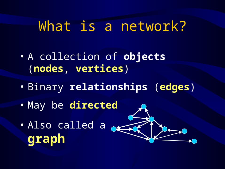
What is a network?
• A collection of objects (nodes, vertices)
• Binary relationships (edges)
• May be directed
• Also called a
graph

Networks are everywhere

Social networks
from www.liberality.org
Nodes:People
Edges:Friendship

Sexual networks
Nodes:People
Edges:Romantic and sexual relations
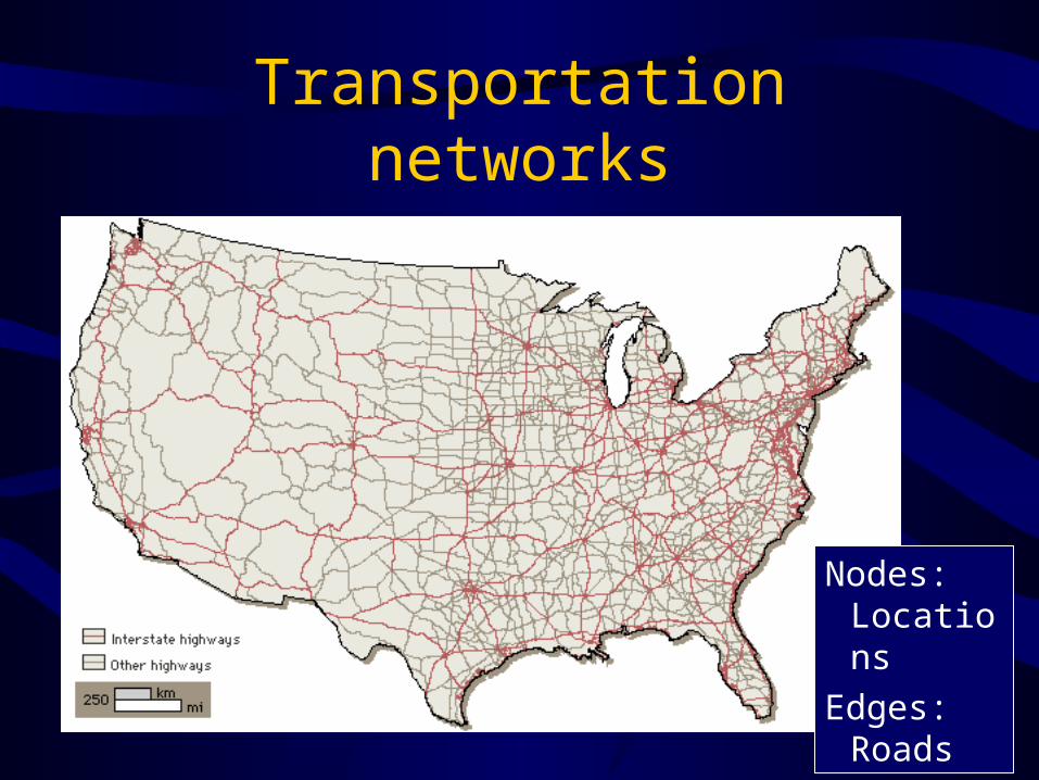
Transportation networks
Nodes:Locations
Edges:Roads

Power grids
Nodes:Power station
Edges:High voltage transmission line

Airline routes
Nodes:
Airports
Edges:
Flights

Internet
Nodes:MBone Routers
Edges:Physical connection

Internet
Nodes:Autonomous systems
Edges:Physical connection

World-Wide-WebNodes:
Web documents
Edges:Hyperlinks
Gene and protein networks

Metabolic networks
Nodes:Metabolites
Edges:Biochemical reaction(enzyme)
from web.indstate.edu
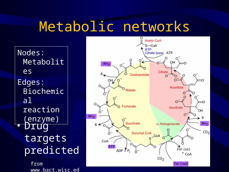
Metabolic networks
• Drug targets predicted
Nodes:Metabolites
Edges:Biochemical reaction(enzyme)
from www.bact.wisc.edu

Metabolic networks
Nodes:Metabolites
Edges:Biochemical reaction(enzyme)

Protein interaction networks
• Gene function predictedfrom www.embl.de
Nodes:Proteins
Edges:Observed interaction

Gene regulatory networks
• Inferred from error-prone gene expression data
from Wyrick et al. 2002
Nodes:Genes or gene products
Edges:Regulation of expression

Signaling networks
Nodes:Molecules(e.g., Proteins or Neurotransmitters)
Edges:Activation orDeactivation
from pharyngula.org

Signaling networks
Nodes:Molecules(e.g., Proteins or Neurotransmitters)
Edges:Activation orDeactivation
from www.life.uiuc.edu

Synthetic sick or lethal (SSL)
Cells live(wild type)
Cells live
Cells live
Cells dieor grow slowly
X
Y
X
Y
X
Y
X
Y

SSL networks
• Gene function, drug targets predicted
Nodes:Nonessential genes
Edges:Genes co-lethal from Tong et al. 2001
X
Y

Other biological networks
• Coexpression– Nodes: genes– Edges: transcribed at same times,
conditions
• Gene knockout / knockdown– Nodes: genes– Edges: similar phenotype (defects) when
suppressed

What they really look like…

We need models!

Traditional graph modeling
Random Regular
from GD2002

Introduce small-world networks

Small-world Networks
• Six degrees of separation
• 100 – 1000 friends each
• Six steps: 1012 - 1018
• But…
We live in communities

Small-world measures
• Typical separation between two vertices– Measured by characteristic path length
• Cliquishness of a typical neighborhood– Measured by clustering coefficient
v
Cv = 1.00
v
Cv = 0.33

Watts-Strogatz small-world model

Measures of the W-S model
• Path length drops faster than cliquishness
• Wide range of phas both small-worldproperties

Small-world measures of various graph types
CliquishnessCharacteristic Path Length
Regular graph High Long
Random graph Low Short
Small-world graph High Short

Another network property: Degree distribution P (k)
• The degree (notation: k) of a node is the number of its neighbors
• The degree distribution is a histogram showing the frequency of nodes having each degree

Degree distribution of E-R random networks
Binomial degree distribution,
well-approximated by a Poisson
Degree = kP
(k)
Erdös-Rényi random graphs
Network figures from Strogatz, Nature 2001
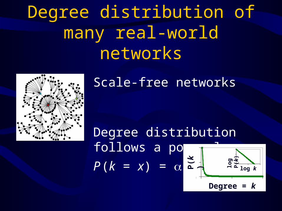
Degree distribution of many real-world networks
Scale-free networks
Degree distribution follows a power law
P (k = x) = x -
Degree = kP
(k)
log klog
P(k
)
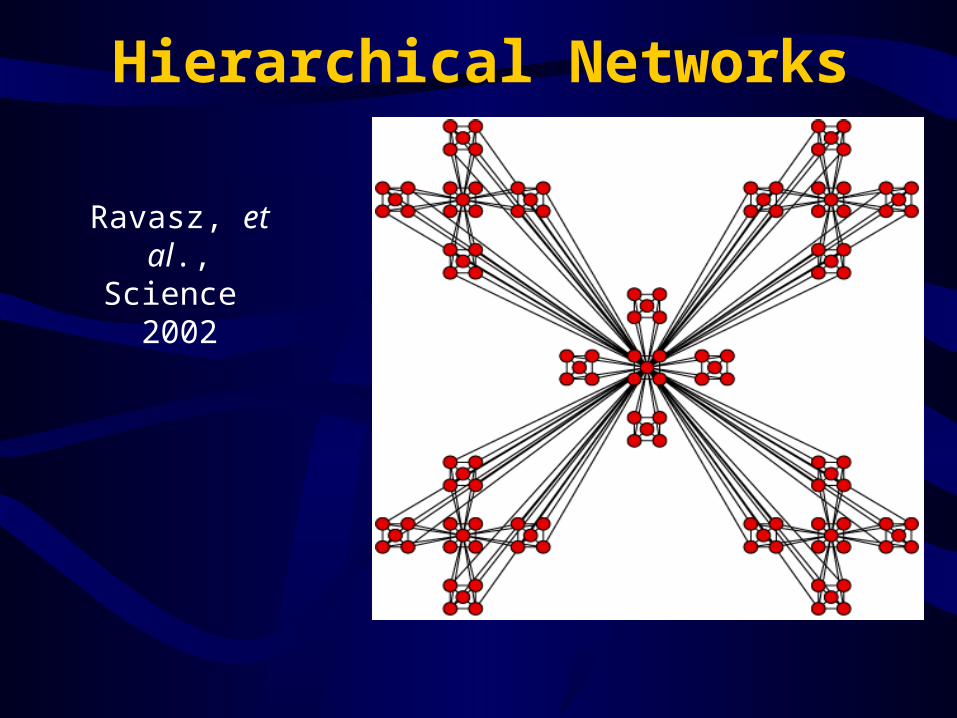
Hierarchical Networks
Ravasz, et al., Science 2002

3. Scaling clustering coefficient (DGM)
2. Clustering coefficient independent of N
Properties of hierarchical networks
1. Scale-free

C of 43 metabolic networks• Independent of N
Ravasz, et al., Science 2002

Scaling of the clustering coefficient C(k)
• Metabolic networks
Ravasz, et al., Science 2002

Many real-world networks are small-world, scale-free
• World-wide-web• Collaboration of film actors (Kevin Bacon)• Mathematical collaborations (Erdös number)• Power grid of US• Syntactic networks of English• Neural network of C. elegans• Metabolic networks• Protein-protein interaction networks


There is information in a gene’s position in the network
We can use this to predict
• Relationships– Interactions – Regulatory relationships
• Protein function– Process– Complex / “molecular machine”
Confidence assessment
• Traditionally, biological networks determined individually– High confidence – Slow
• New methods look at entire organism– Lower confidence ( 50% false positives)
• Inferences made based on this data

Confidence assessment
• Can use topology to assess confidence if true edges and false edges have different network properties
• Assess how well each edge fits topology of true network
• Can also predict unknown relations
Goldberg and Roth, PNAS 2003

Use clustering coefficient, a local property
• Number of triangles = |N(v) N(w)|
• Normalization factor?
N(x) = the neighborhood of node x
yx
v
w
v
w ...

Mutual clustering coefficient
Jaccard Index: Meet / Min: Geometric:
|N(v) N(w)|----------------|N(v) N(w)|
|N(v) N(w)| 2
------------------ |N(v)| · |N(w)|
|N(v) N(w)|------------------------min ( |N(v)| , |N(w)| )
Hypergeometric:
a p-value

Mutual clustering coefficient
Hypergeometric:P (intersection at least as large by chance)
-log
= neighbors of node v
= neighbors of node w
= nodes in graph

Prediction
• A v-w edge would have a high clustering coefficient
v
w

Confidence assessment
• Integrate experimental details with local topology– Degree– Clustering coefficient– Degree of neighbors– Etc.
Bader, et al., Nature Biotechnology 2003

The synthetic lethal network has many triangles
Xiaofeng Xin, Boone Lab

2-hop predictors for SSL
• SSL – SSL (S-S)• Homology – SSL (H-S)• Co-expressed – SSL (X-S)• Physical interaction – SSL (P-S)• 2 physical interactions (P-P)
v
w
S: Synthetic sickness or lethality (SSL)H: Sequence homologyX: Correlated expressionP: Stable physical interaction
Wong, et al., PNAS 2004

Multi-color motifs
Hir1
Hhf1 Hht1
RR
P,X
C2C1 C2C1
Nrand:
Nreal:
(3.6+0.2) ×103(4.3+0.5)×102
1.5×1045.6×103
Nrand:
Nreal:
(3.6+0.2) ×103(4.3+0.5)×102
1.5×1045.6×103
R R
P
R R
X
a
b c
RR
P/X
Hir1 Hir2
Hhf1
Hhf2 Hht2
Hht1
Htb1
Htb2Hta2
Hta1Motif Set C
a network motif a network theme
Hir1
Hhf1 Hht1
RR
P,X
C2C1 C2C1
Nrand:
Nreal:
(3.6+0.2) ×103(4.3+0.5)×102
1.5×1045.6×103
Nrand:
Nreal:
(3.6+0.2) ×103(4.3+0.5)×102
1.5×1045.6×103
R R
P
R R
X
a
b c
RR
P/X
Hir1 Hir2
Hhf1
Hhf2 Hht2
Hht1
Htb1
Htb2Hta2
Hta1Motif Set C
a network motif a network theme
Hir1
Hhf1 Hht1
RR
P,X
C2C1 C2C1
Nrand:
Nreal:
(3.6+0.2) ×103(4.3+0.5)×102
1.5×1045.6×103
Nrand:
Nreal:
(3.6+0.2) ×103(4.3+0.5)×102
1.5×1045.6×103
R R
P
R R
X
a
b c
RR
P/X
Hir1 Hir2
Hhf1
Hhf2 Hht2
Hht1
Htb1
Htb2Hta2
Hta1Motif Set C
a network motif a network theme
S: Synthetic sickness or lethalityH: Sequence homologyX: Correlated expressionP: Stable physical interactionR: Transcriptional regulation
Zhang, et al., Journal of Biology 2005

SSL “hubs” might be good cancer drug targets
(Tong et al, Science, 2004)
Normal cell Cancer cells w/ random mutations
Alive Dead Dead

Predict protein function from function of neighboring proteins
• “Guilt by association”
• Consider immediate neighbors– Schwikowski, et al., Nature Biotechnology
2001
• Consider a given radius– Hishigaki, et al., Yeast 2001

Predict protein function from neighboring proteins (2)
• Minimize interactions between proteins with different annotations– Vazquez, et al., Nature Biotechnology 2003– Karaoz, et al., PNAS 2004
• Use network flow algorithm to “transport” function annotation– Nabieva, et al., Bioinformatics 2005

Lethality
• Hubs are more likely to be essential
Jeong, et al., Nature 2001

Degree anti-correlation
• Few edges directly between hubs
• Edges between hubs and low-degree genes are favored
Maslov and Sneppen, Science 2002

Beware of bias

Protein abundance
• Abundant proteins are – more likely to be represented in some
types of experiments– More likely to be essential
• Correlation between degree (hubs) and essentiality disappears or is reduced when corrected for protein abundance
Bloom and Adami, BMC Evolutionary Biology 2003

Degree correlation
• Anti-correlation of degrees of interacting proteins disappears in un-biased data
Coulomb, et al., Proceedings of the Royal Society B 2005
0 10 20 30 40 50 60 70
degree k
aver
age
degr
ee K
1
25
20
15
10
5
0
essential
non-essential
Community structure
Partitioning methods
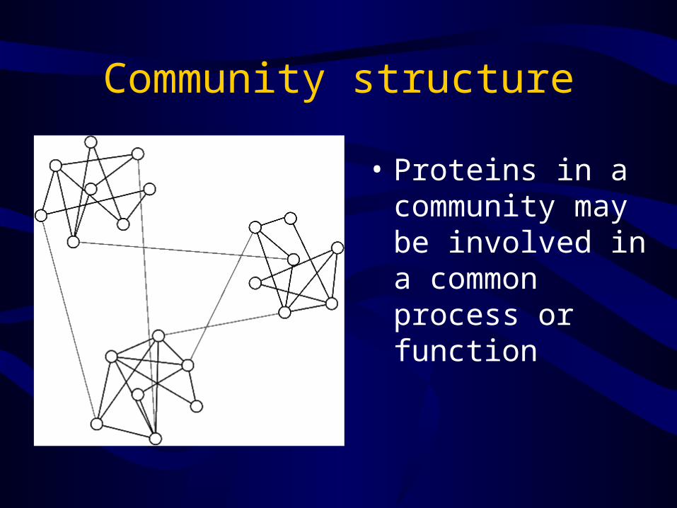
Community structure
• Proteins in a community may be involved in a common process or function

Finding the communities
• Hierarchical clustering
• “Betweenness” centrality
• Dense subgraphs
• Similar subgraphs
• Spectral clustering
• Party and date hubs

Hierarchical clustering (1)Using natural edge weights
• Gene co-expression
• e.g., Eisen MB, et al., PNAS 1998
from www.medscape.com

Hierarchical clustering (2)Topological overlap
• A measure of neighborhood similarity
li,j is 1 if there is a direct link between i and j, 0 otherwise
Ravasz, et al., Science 2002

Hierarchical clustering (3)Adjacency vector
• Function cluster: Tong et al., Science 2004
• Find drug targets: Parsons et al., Nature Biotechnology 2004

“Betweenness” centrality
• Consider the shortest path(s) between all pairs of nodes
• “Betweenness” centrality of an edge is a measure of how many shortest paths
traverse this edge
• Edges between communities have higher centrality
Girvan , et al., PNAS 2002
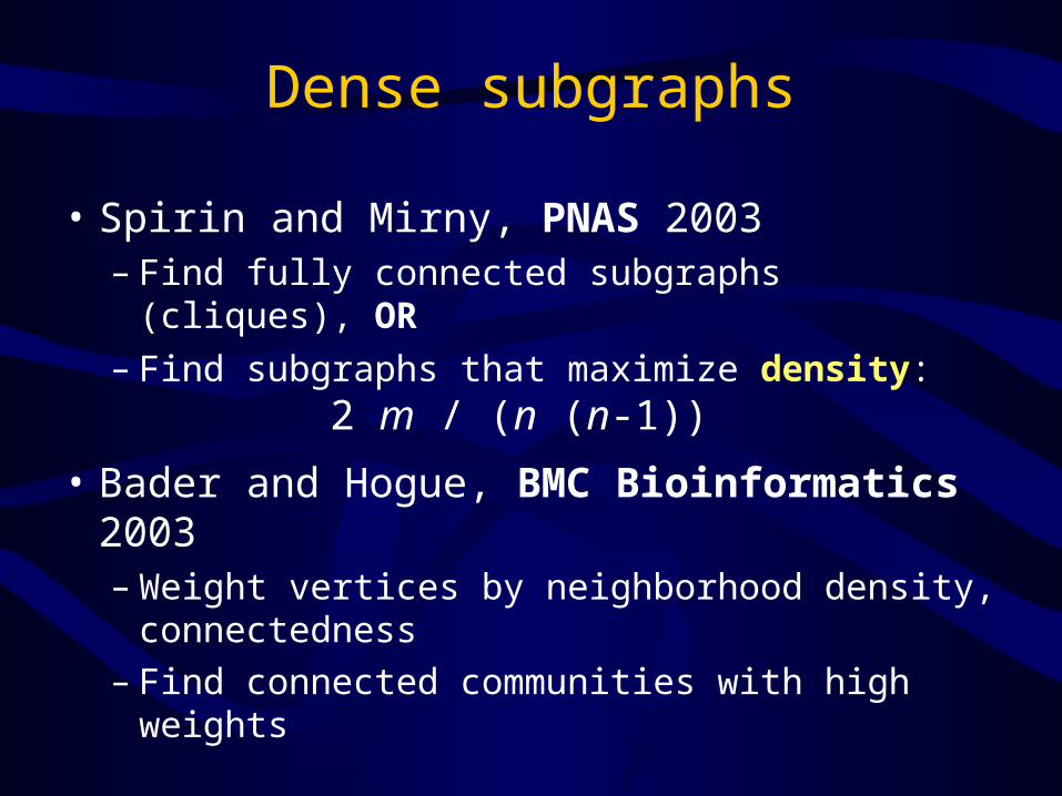
Dense subgraphs
• Spirin and Mirny, PNAS 2003– Find fully connected subgraphs (cliques), OR
– Find subgraphs that maximize density: 2 m / (n (n-1))
• Bader and Hogue, BMC Bioinformatics 2003– Weight vertices by neighborhood density,
connectedness– Find connected communities with high weights

Similar subgraphs
• Across species
• Interaction network and genome sequence
• e.g., Ogata, et al., Nucleic Acids Research 2000

Spectral clustering
• Compute adjacency matrix eigenvectors
• Each eigenvector defines a cluster:– Proteins with high magnitude contributions
Bu, et al., Nucleic Acids Research 2003
positive eigenvalue negative eigenvalue

Party and date hubs
• Protein interaction network
• Partition hubs by expression correlation of neighbors
Han, et al., Nature 2004

Network connectivity
• Scale-free networks are: – Robust to random failures– Vulnerable to attacks on hubs
• Removing hubs quickly disconnects a network and reduces the size of the largest component
Albert, et al., Nature 2000

Removing date hubs shatters network into communities
Many sub-networks
Date Hubs
Party Hubs
A single main component

Temporal partitioning
Luscombe, et al., Nature 2004
Final words
• Network analysis has become an essential tool for analyzing complex systems– There is still much biologists can learn from
scientists in other disciplines
• The references mentioned are representative, and not comprehensive